Atmospheric Carbon Dioxide: A Fresh Look at Exchange Flux, Isotopic Carbon, Fossil Fuel Emissions and Residence Time

1. Introduction

The absolute (gross) size of the atmospheric CO₂ exchange flux between the atmosphere and the land/ocean are crucial in understanding the carbon cycle and estimating the effects of anthropogenic CO₂ fossil fuel emissions (CO2ff). As the Earth rotates daily and orbits the sun annually, the land and oceanic reservoirs cyclically "inhale" and "exhale" CO₂. These are the exchange fluxes, caused by corresponding changes in temperature, seawater solubility, photosynthesis, plant decay and respiration, resulting in a continuous cycle of absorption and emission. Within this complicated pattern of two-way fluxes, absorption occurs at one geographical location while simultaneously emitting at another. (IPCC Ed., 2001) This paper presents a means of determining the gross exchange flux. Measuring the gross exchange flux is more difficult than the task of finding its nett value, since the gross value does not contribute to the global carbon budget. Current estimates by the Global Carbon Budget (GCB) are for the land exchange flux 130 GtC yr^-1, and for the ocean flux 80 GtC yr^-1 (Friedlingstein et. al., 2022). GCB refers its data source as being IPCC Canadell 2021 (IPCC Ed., 2021) who indicate that for the ocean, the gross figures originate from Figure 1 of Sarmiento & Gruber 2002 with applied corrections. Earlier GCB reports refer to IPCC (Ed) 2013 which states "Individual gross fluxes and their changes since the beginning of the Industrial Era have typical uncertainties of more than 20%" (author's highlight).

In the 1970s attempts were made to model the carbon cycle and exchange flux using box models (e.g. Oeschger et al., 1975). Subsequently, General Circulation Models (GCMs) became common, since they could create global geographical distribution maps of the carbon-related processes despite requiring more computer resources. Although GCMs have been helpful in understanding the complexity of the global carbon cycle, box models, with their top-down simplification, offer specific advantages over the open-ended micro-accounting of GCMs. Such simpler models are "better testable" (Popper, 1934) and can help identify errors in formulation by focusing on the most significant factors. This paper presents a 2-box model that computes ¹⁴C and ¹³C isotopic ratios and differs from other box models in several ways. Firstly, its uses atmospheric CO₂ levels as input rather than output. Secondly, it employs absolute flow instead of net flow. Lastly, it incorporates a factor describing the proportion of fossil fuel emissions that are directly absorbed by sinks before dilution in the atmosphere takes place. The model accurately calculates ¹⁴CO₂ and ¹³CO₂ isotopic ratios spanning over 200 years, including the bomb pulse. Yet, notably, it uses the same residence time and reservoir mixing properties for ¹⁴C, ¹³C and ¹²C.

In addition to uniquely providing estimates of the magnitude of the exchange flux, the method also challenges the widely held view that "the atmospheric impulse response function of an isotopic perturbation decays much more rapidly than the impulse response function for bulk carbon" (Heimann 1993). See Discussion Section 5.

1.1. Radiocarbon

The isotopic abundance of ¹³C and ¹⁴C present within atmospheric CO₂ is accurately known globally, with records going back hundreds of years. These isotopes have been measured in samples from tree rings (Stuiver & Quay 1981), ice cores (Rubino et al., 2013), and the atmosphere (Stuiver et al., 1998; D6). While ¹³C is radioactively stable and forms around one percent of atmospheric carbon, ¹⁴C undergoes radioactive decay with a half-life of 5700 ± 30 years (Kutschera 2013), and comprises about 1 part in 10¹². There is virtually no presence of ¹⁴C in fossil fuel since it has all radioactively decayed. The ¹⁴C/¹²C ratio decreased between 1800 and 1960 because of dilution from rising fossil fuel emissions which are ¹⁴C depleted, a process known as "Suess dilution" (Suess 1955). In 1960, atmospheric nuclear weapons testing began, causing a doubling of the absolute ¹⁴C level within ten years. Since 1975 the level of ¹⁴C has decreased (D6), partially due to washout from the exchange flow which contains a somewhat lower level of ¹⁴C, but also because of "Suess dilution". Turning now to ¹³C, its presence in fossil fuels is reduced when compared with the atmosphere, but only by around 2% (Stuiver and Polach, 1977). This small reduction arises from fractionation, which means the larger less mobile isotopic CO₂ molecules are less likely to become embedded in leaves and fossil carbon. Measurements show that the atmospheric ¹³C/¹²C ratio has decreased during the past 200-year period (D4), again partially due to dilution by fossil fuel carbon which contains the lower level of ¹³C, and partially because of washout from the exchange flow. See Section 4.2.

2. CO₂ Absolute Flow Finite Reservoir Model

The model calculates the movement of CO₂ and its carbon isotopes between the atmosphere and a mixing reservoir, by calibration against isotopic measurements. The size of this mixing reservoir, and the exchange flux are "effective" values, combining the effect of the ocean and terrestrial origins. The concept of effective values is commonplace in the fields of engineering, applied science and economics. For example, economic inflation represents, in a single figure, the average of many different price increases on many items. Productivity measures the effective value created by each hour of work. Effective resistance in electronic engineering or hydraulics gives the overall resistance of a complex system to current or fluid flow. In each of these examples a single value is used to account for a property which is distributed throughout a complex system. The model presented is able to determine the effective values without requiring a detailed audit of the underlying constituent components, unlike other methods. 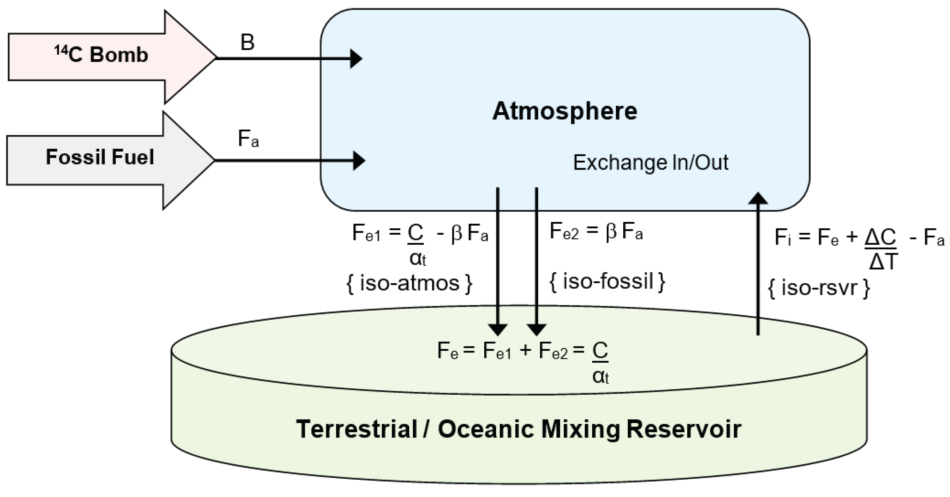The model consists of two boxes which are considered well-mixed, Figure 1. At each annual iteration, the isotopic mixing ratio within the reservoir and atmosphere changes because of incoming ¹³C and ¹⁴C. This change is calculated by the dilution formulae in Section 2.1. Using a similar notation as Tans et al.(1993) and Cawley (2011) we have

dC/dT = F_a + F_i - F_e

(1)

where C is the atmospheric carbon mass, F_a is the anthropogenic input flux from fossil fuel emissions, F_i, is the environmental flux flowing into the atmosphere and F_e is the environmental flux exiting the atmosphere. It is essential that F_i and F_e are kept separate because inflow and outflow are occurring in different places and they are needed to calculate the isotopic flows. Summing these components to form a nett flow would lose track of the separate isotopic mixing occurring across the globe.

Figure 1. CO₂ Finite Reservoir Two-Box Model. The model describes the CO₂ flux between the reservoir and atmosphere, including its isotopic carbon contents. Anthropogenic fossil fuel CO2ff F_a, enters the atmosphere and a portion β exits without mixing. The remaining portion, (1-β) mixes into the atmosphere. Otherwise, full isotopic mixing is assumed to occur within each of the two storage regions, atmosphere and reservoir. At each iteration, the CO₂ flux outflow, F_e is proportional to atmospheric CO₂, C(t); its isotopic level corresponds to a mixture of atmospheric and fossil content. The CO₂ influx, F_i is determined by using equation (1) below. Atomic weapons ¹⁴C B(t) directly enters the atmosphere with the timing and amounts determined by historical records of individual atmospheric atomic weapons testing, and bomb yield.

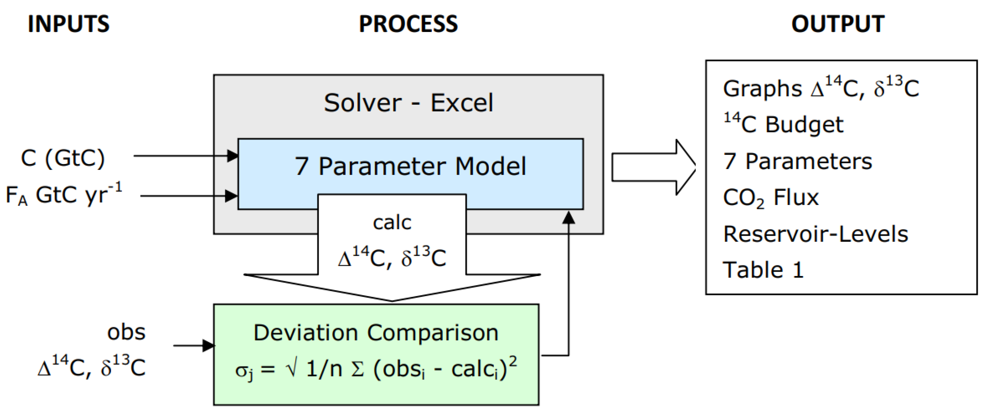
Figure 1. CO₂ Finite Reservoir Two-Box Model. The model describes the CO₂ flux between the reservoir and atmosphere, including its isotopic carbon contents. Anthropogenic fossil fuel CO2ff F_a, enters the atmosphere and a portion β exits without mixing. The remaining portion, (1-β) mixes into the atmosphere. Otherwise, full isotopic mixing is assumed to occur within each of the two storage regions, atmosphere and reservoir. At each iteration, the CO₂ flux outflow, F_e is proportional to atmospheric CO₂, C(t); its isotopic level corresponds to a mixture of atmospheric and fossil content. The CO₂ influx, F_i is determined by using equation (1) below. Atomic weapons ¹⁴C B(t) directly enters the atmosphere with the timing and amounts determined by historical records of individual atmospheric atomic weapons testing, and bomb yield.

We first need an expression which connects the atmospheric CO₂ mass C, to the outflow; F_e is an obvious choice, being

F_e = a C

(2)

Equation(2) meets the common sense requirements that the absolute exchange exit flux varies in proportion to C, and if C were to be zero, the exit flux, F_e would also be zero. Substituting (2) into (1), we obtain an ordinary differential equation (ODE) for absolute inflow as

F_i = a C + dC/dT - F_a

(3)

The formula also describes the analogous situation of the flow of water from a bucket with a hole of size related to a, and two input taps (faucets) one of which represents the environmental exchange inflow, F_i and the other represents fossil fuel inflow, F_a. In practice, for use with data series, we replace dC/dt with ΔC/ΔT where ΔC is the difference of successive carbon atmospheric mass and ΔT is the time difference, leading directly to the implementation equations shown in Section 2.4. The formulation differs from those used by other authors in two important respects. First, the incoming flux, F_i is not assumed constant and is calculated at each iteration by "balancing the books". Second, F_e is calculated by direct proportionality to the atmospheric CO₂ mass. As a consequence the model is not a predictive model of CO₂ atmospheric level. However, a great advantage of this formulation is that it enables the inflow to be calculated from measured data, eliminating the need to provide a bottom-up audit of individual CO₂ sources. Furthermore it provides estimates of CO₂ inflow and CO₂ isotopic ratios, and it computes a value for the CO₂ residence time constant. This constant applies equally to all three carbon species ¹⁴CO₂, ¹³CO₂ and ¹²CO₂. See Section 5.0 for further discussion.

The model uses a bomb yield multiplication factor, Y_b, as one of its seven optimisation parameters, to calculate the nuclear bomb yield of ¹⁴C each year, B₁₄[i]. The bomb yield in megatons is obtained from records of atomic weapons atmospheric test detonations [D5]. A simple time delay of one year was used to allow for atmospheric mixing. The initial values i.e. δ¹³C_init, Δ¹⁴C_init, are also optimisation parameters within the model and determine the initial level of the curves in Figure 3 & Figure 4, while the parameter δ¹³C_FF determines the curve slopes in Figure 5.

2.1. Mass-Balance and Isotopic Dilution

If a number of gases are mixed but do not react, and each component gas, i, has a mass M_i, then from the law of conservation of mass (also known as Mass Balance)

MT = Σ Mi

If within each component gas there is a specific molecule present in a ratio to its mass, R_i, then, since that specific molecule is conserved, the resulting mixture (e.g. paint mixing) having mass M_T has a ratio R_T given by

RT = Σ Ri Mi / MT

(4)

Equation(4) also applies to the situation of mixing of isotopic gases. For practical reasons associated with historical measurements of radioactivity, studies of isotopic mixtures normally utilize the ratio of the sample activity, A_S to a standard sample activity A_abs, this ratio being known as the relative specific activity, A. Its value is then offset by one to provide the radioactivity scale, δ written (see Strenstrom 2011) in the form

δ = (A_s/A_abs) -1 = A - 1

(5)

In this scale, although δ increases linearly with As, its value is offset to be zero at the value of the absolute standard (often chosen to approximate background level), as for example in the cases of δ13C and δ14C. Applying (5) and substituting ASi for each component Ri of the mixture, leads after some algebraic manipulation, to

δ_T = Σ (δ_i M_i ) / M_T

(6)

The similarity with equation(4) shows that although δ is defined by an offset ratio scale we can still directly apply equation(6) to calculate the resulting value of δ_T for the mixture. The above scheme forms the basis for the system of equations A₁₄[], R₁₄[], A_FF[] and R_FF[] shown in the implementation Section 2.4 below.

2.2. Fractionation

The model generates values of δ¹⁴C, but we require Δ¹⁴C for comparison with observed Δ¹⁴C values. Δ¹⁴C incorporates a fractionation correction to "translate the measured activity to the activity the sample would have had if it had been wood" (Strenstrom 2011). The correction formulae, which are themselves a function of δ¹³C, may be derived from equations by Strenstrom 2011 using equations 25, 28, 38, or Stuiver & Polach 1977 p356, 360, Table 1, where A_SN is the normalised specific sample activity, A_s is the specific activity of the atmosphere or reservoir, A_abs is the absolute specific standard, δ¹³C_M is the ¹³C sample measurement, and δ¹³C_W is the ¹³C standard for wood, giving

δ14C = AS / Aabs - 1

Δ14C = ASN / Aabs - 1

ASN = AS [ ( 1 + δ13CW) / ( 1 + δ13CM) ]2

Eliminating A_S , A_abs and A_SN gives

Δ¹⁴C = [1 + δ¹⁴C ] [ (1 + δ¹³C_W) / (1 + δ¹³C_M) ]² - 1

The above formula was used to convert values of δ¹⁴C computed by the model to Δ¹⁴C. The standard value of δ¹³C for wood was taken as 25‰, while δ¹³C_M was taken from the model. The correction was small, approximately 10‰ when the bomb pulse has a peak value of 800‰, decreasing to 0.03‰ when δ¹⁴C approaches its background value of zero.

2.3. Age Correction

The radioactive decay of ¹⁴C over the period from 1820 to 2020 is approximately 2%, since its half-life is 5700 ±30 years (Kutschera, W., 2013). However, this relatively small value is even less significant when one considers that the steady production of stratospheric ¹⁴C approximately balances the amount of ¹⁴C decay, since the two are in quasi-equilibrium. Therefore, neither ¹⁴C decay nor natural stratospheric ¹⁴C production were included in the model.

2.4. Implementation

Using equations 1-3 for the amount of CO₂ in the atmosphere C, its removal time α_t, the atmosphere outflow F_e, the inflow F_i, and the amount of CO₂ in the reservoir R, with the square brackets '[i]' referring to the value at each iteration i, we have

• F_e[i] = C[i] /α_t , F_e2[i] = β F_a[i] ,F_e1[i] = F_e[i] - β F_a[i]
• F_i[i] = F_e [i] + C [i] - C [i-1] - F_a [i-1] ,R[i] = R [i-1]+ F_e[i] - F_i[i]

The ratio of ¹⁴C to C in the atmosphere is denoted by A₁₄ and in the reservoir by R₁₄ and is calculated as follows. The new amount is given by the previous amount added to the input amounts with the output amount being subtracted, all divided by the total mass (see equation 4). If necessary we include the annual ¹⁴C production due to atomic weapons bomb input, B₁₄. Hence we obtain

• A₁₄[i] = (A₁₄[i-1] . C[i-1] + F_i[i-1].R₁₄[i-1] - F_e[i-1].A₁₄[i-1] + B₁₄[i-1]) / C [i]
• R₁₄[i] = (R₁₄[i-1] . R[i-1] - F_i[i-1].R₁₄[i-1] + F_e1[i-1].A₁₄[i-1] ) / R [i]

Similarly, the relative atmospheric and reservoir fossil fuel content A_FF and R_FF, are calculated on a scale of 0 to 1 using the values at the previous iteration levels, where A refers to the atmosphere, and R the reservoir and subscripts FL means fossil fuel level, and NL means natural non-fossil level,

• A_FF[i] = (A_FF [i-1].C[i-1] + F_i[i-1].R_FF [i-1] - F_e1[i-1].A_FF[i-1] - F_e2[i-1] + F_a [i-1])/C [i]
• R_FF[i] = (R_FF [i-1].R [i-1] - F_i[i-1].R_FF [i-1] +F_e1[i-1].A_FF[i-1] + F_e2[i-1]) / R [i]
• A_FL[i] = C[i] A_FF[i], A_NL[i] = C[i] - A_FF[i]
• R_FL[i] = R[i] R_FF[i] , R_NL[i] = R[i] - R_FF[i]

The offset isotopic ratiometric measure for ¹³C is δ¹³C and that for ¹⁴C is Δ¹⁴C. These are calculated from the iterative series by:-

δ¹³C = δ¹³C_FF . A_FF + δ¹³C_N (1 - A_FF), Δ¹⁴C = (A₁₄ -1)

Initial Conditions: F_i[0] = F_e[0] , A₁₄ [0] = 1 , R₁₄ [0] = 1, A_FF[0] = 0 , R_FF[0] = 0

It is not necessary to embed a formula for attenuation factor, as discussed by Stuiver & Quay (1981), or for Suess dilution (Suess 1955) because they are implicitly represented.

3. Method

The input data between 1750 and 2020 was selected from the appropriate data source listing (D1-D6) and entered into a spreadsheet. The cell formulae were set to correspond to those equations in Section 2.4

The optimisation-solution process is shown in Figure 2 above. The standard deviation between observed and predicted values, σ₁, σ₂ were determined for Δ¹⁴C and δ¹³C respectively. The values of Δ¹⁴C between 1950 and 1968 were excluded from the summation because of the bomb pulse transient. The square root of the product of the standard deviations gives the overall geometric mean standard deviation, σ_Τ, hence

σ_j = √ 1/n Σ (obs_i - calc_i)²

(7)

σ_Τ = (σ₁ x σ₂ )^1/2

(8)

The solver system was set to optimise the 7 parameters shown in Table 1 using the default solver options. The optimal solution was found by minimizing the discrepancy, σ_Τ using the standard "Solver" function of Microsoft Excel. The model has been tested using Microsoft Excel 2002 Version 10 and Microsoft Excel for Microsoft 365 MSO Version 2306 producing identical results.

4. Results

The results are in three main categories; the optimised seven parameters, the isotopic series, and the flux time series.

4.1. Parameter Values

Table 1 lists all seven parameter values along with their estimated errors. The error values were derived by varying each parameter up and down, while keeping the other parameter values constant, until the overall geometric mean standard deviation, σ_Τ approximately doubled. The error figure presented in the table is the mean of the two variations.

1) Residence Time

This compares favourably with Revelle & Suess (1957) of approximately 10 years, and Arnold (1957) of 10-20 years. It has subsequently been stated that "No single lifetime can be defined for CO₂.." (IPCC (Ed.): 2001, Table 1 p38). This study finds to the contrary.

2) Reservoir Size rel. to Atmosphere (1750)

The value for reservoir size are reported in IPCC Ed., (2013) in GtC as vegetation 450 to 650, soils 1500 to 2400, permafrost 1700, and surface ocean 900, corresponding to a range of 4550 to 5650. This study finds a reservoir size in GtC of 6.18 x 589 = 3640 GtC increasing to 3809 GtC in 2020 with errors of +/- 22%.

3) CO₂ Relative Unmixed Uptake

This study determines the quantity of CO2ff entering the sink without mixing in the atmosphere. Factor β accounts for the unmixed uptake, corresponding to that portion of the CO2ff emissions which directly enter the terrestrial/oceanic mixing reservoir. The effect of entry of pure undiluted CO2ff is a lowering of the ¹⁴C and ¹³C curves. The model finds that around 43% of CO2ff exits before mixing while 57% becomes fully mixed. A recent study has revealed that plants near nuclear power stations can uptake significant quantities of ¹⁴CO₂ (Naegler & Levin 2006). A study of urban grasses near a major highway revealed plants were composed of up to 13% of fossil-fuel carbon (Lichtfouse et al, 2005; Ota et al 2016). According to Kuderer et al (2018), "The 14C signals from such point sources are well detectable in plant samples". Since most fossil fuel emission sources are located near the land or ocean surface, it is reasonable to propose that a significant portion of CO₂ fossil fuel emissions are absorbed before fully mixing in the atmosphere.

4) Nuclear Bomb Yield

The model returned a value of 1.6 ± 0.1‰ of ¹⁴C per MT for the nuclear bomb yield, with a total bomb yield of 440MT. For comparison, we convert the figures to ¹⁴C atoms per MT bomb yield using formulae derived from Svetlik (2010) and Strensom (2011). The weight of carbon atoms, A_CO2 in the atmosphere in 1950, when the CO₂ mixing-ratio was 312.8 ppm, was 664.43 GtC. The number of carbon atoms is given in terms of the molecular weight of naturally abundant carbon, MC = 12.01, and Avogadro's number N_A = 6.022×10²³ by

NC = A_CO2 x N_A / MC.

The ¹⁴C/C ratio R¹⁴C can be obtained from the specific activity, α = 0.226 Bq per gram, ¹⁴C half life T_1/2 = 5730 years = 1.807 10¹¹ s, molar weight of ¹⁴C is M_C14 = 14, and ln(2) = 0.6931, with

R¹⁴C = α T_1/2 M_C14 / (N_A x ln(2)).

The number of ¹⁴C atoms N¹⁴C created is given by the product of the two expressions giving

N¹⁴C = NC x R¹⁴C = (A_CO2 / MC) x ( α T_1/2 MC₁₄ / ln(2)) = 4.6 x 10²⁸.

Hence the number of 14C atoms per MT of bomb yield is 0.0016 x 4.6 x 10²⁸ = 7.4 x 10²⁵, comparing favourably with reported values by Hesshaimer et al. (1994) of 1 to 2 x 10²⁶ atoms per MT. The total bomb yield of 440MT gives a figure of 3.23 x 10²⁸ atoms per MT, which compares with 6.1 x 10²⁸ atoms per MT by Naegler & Levin (2006). The difference may be due to ¹⁴C which is stored but does not mix in the biosphere or because of variation in bomb type and design.

5) Isotopic Pre-Industrial Levels and Fossil Fuel Content

  a) ¹⁴C shows good agreement with Intcal20[D6] for 1820 of 0.7‰. For comparison the maximum level between 1820-2020 is 800‰.

  b) ¹³C initial value, shows excellent agreement with Rubino (2013) 1820 of δ¹³C = 6.7‰.

  c) δ¹³C for CO2ff is slightly low as compared to figures reported by Stuiver & Polach (1977) for coal of δ¹³C = -23 ‰.

4.2. Isotopic Time Series

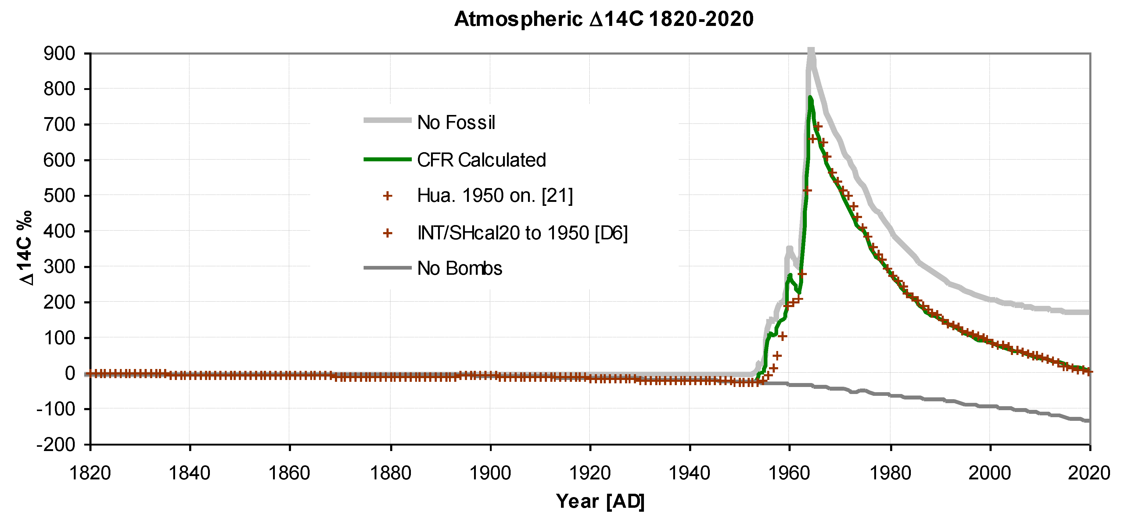
Figure 3 & Figure 4 display the actual and modelled ∆¹⁴C values. The total number of observed data points used was 340, resulting in an overall standard deviation of 0.39‰. The quality of the fit is excellent, with a standard deviation of 3‰, corresponding to 0.4% of the range. In Figure 3, the slight decrease from 1820 to 1940 is due to Suess dilution, but the magnitude of the dilution is somewhat reduced by reservoir inflow, resulting in excellent agreement with the observations. 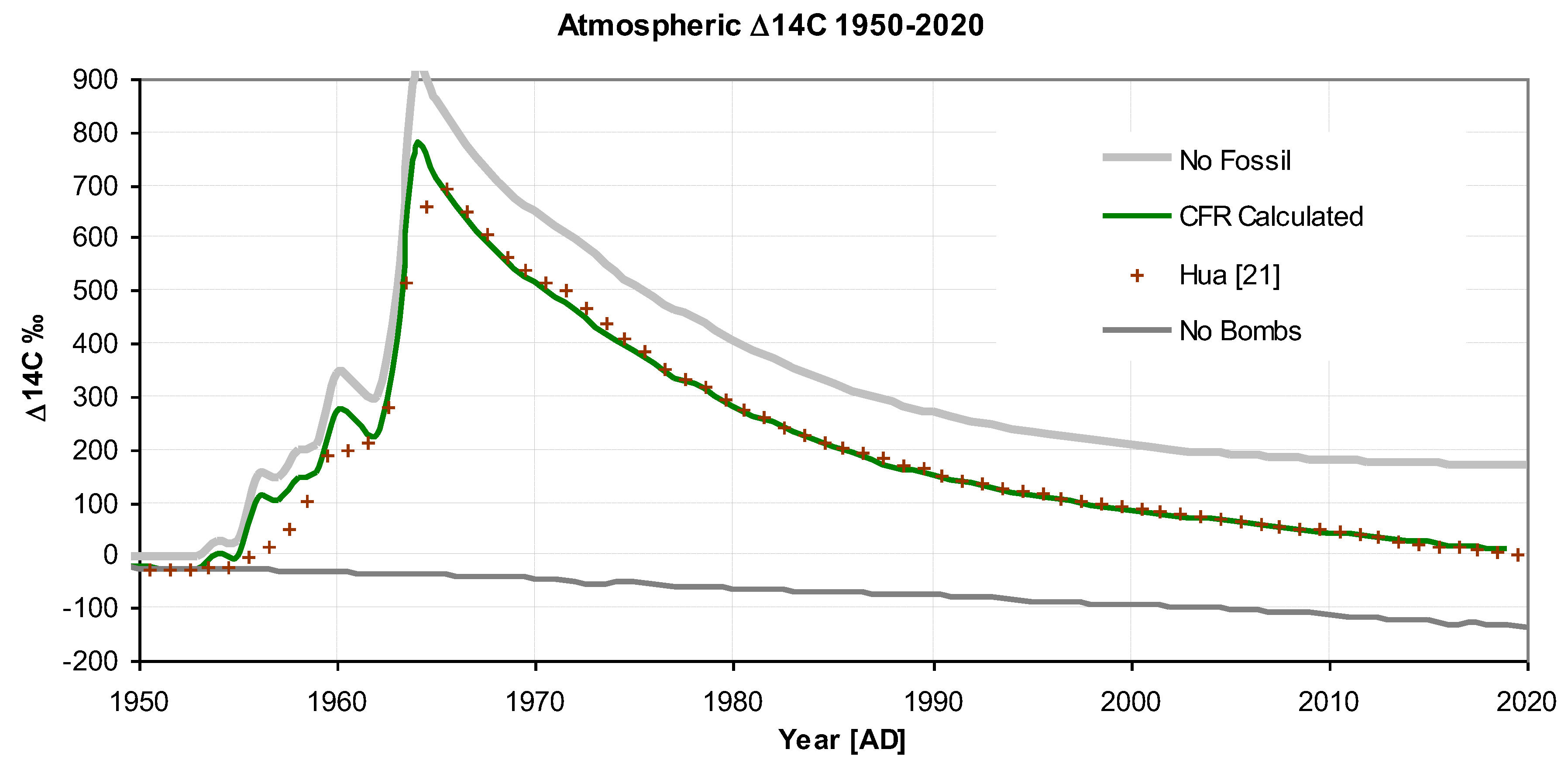Figure 4 shows the bomb pulse plotted as ∆¹⁴C. Initially, the pulse shape is a decaying exponential but, subsequently, due to Suess dilution and the re-emergence of ¹⁴C from the mixing reservoir, the Δ14C decay shape becomes more linear. Despite these complicating factors, the predicted and observed values are in excellent agreement, indicating that the iteration formulae accurately handle the dilution and mixing processes. Figure 3 and Figure 4 also show two hypothetical scenarios: "no bombs" and "no fossil". The "no bombs" scenario represents how the decrease would have continued without nuclear atmospheric weapons testing, while "no fossils" shows the situation without fossil fuel emissions. A recent work published by Graven et al. 2020 using a model originally produced by M. Heimann and R. Keeling and rewritten for Matlab, gave very similar results for "no bombs" and "no fossil" scenarios, further vindicating the model presented here and its approach.

Figure 3. Atmospheric Δ¹⁴C 1820-2020. showing 130 values before 1950 [D6] and 70 values from 1968 onwards (Hua et al.. 2022). Standard deviation between observed and predicted is σ = 3.01‰. For "no bombs" and "no fossil" see text.

Figure 3. Atmospheric Δ¹⁴C 1820-2020. showing 130 values before 1950 [D6] and 70 values from 1968 onwards (Hua et al.. 2022). Standard deviation between observed and predicted is σ = 3.01‰. For "no bombs" and "no fossil" see text.

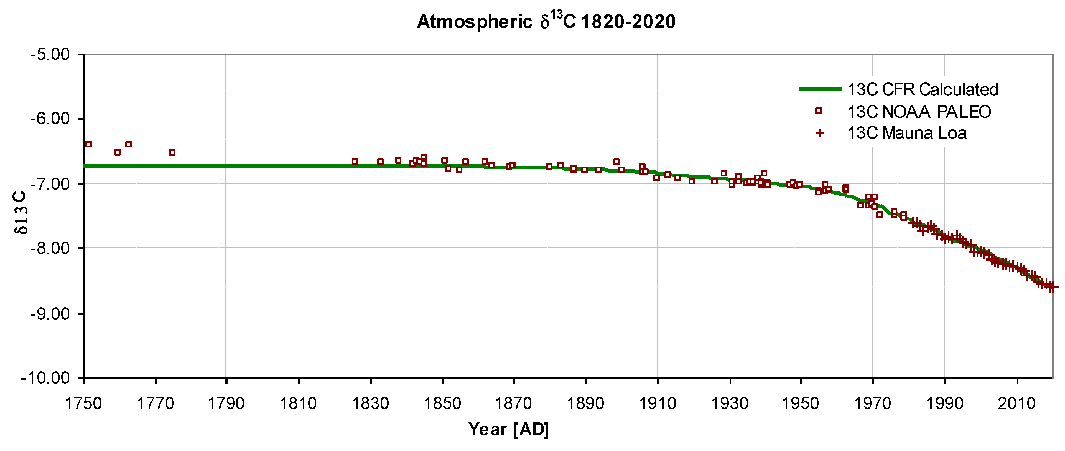
Figure 5 shows the variation of δ¹³C over 200 years, with predicted values showing a standard deviation of 0.05‰ from those observed, corresponding to 2.5% of the range. The steady reduction in δ¹³C is caused by Suess dilution as fossil fuel emissions contain a lower level of ¹³C, and by the re-emission of CO₂ from the reservoir. Again, this shape is accurately described by the iteration formulae.

Figure 4. Atmospheric Δ14C between 1950 and 2020 showing the "bomb pulse" to 2020. For "no bombs" and "no fossil" see text.

Figure 4. Atmospheric Δ14C between 1950 and 2020 showing the "bomb pulse" to 2020. For "no bombs" and "no fossil" see text.

Figure 5. Atmospheric δ13C 1820-2020. Model calculated values: solid green, Observed NOAA Paleo [D4]: squares, Mauna Loa [D2]: crosses, σ_1820-2020= 0.05‰.

Figure 5. Atmospheric δ13C 1820-2020. Model calculated values: solid green, Observed NOAA Paleo [D4]: squares, Mauna Loa [D2]: crosses, σ_1820-2020= 0.05‰.

Inspection of the curve in Figure 4 reveals that atmospheric ∆¹⁴C is decreasing to a value below its original background level. This decrease deviates from an exponential decay due to three main factors. a) Incoming fossil fuel emissions (free of ¹⁴C) are diluting the atmosphere, this is commonly referred to as "Suess Dilution" (Suess 1955). b) Some of that fossil fuel emissions in the atmosphere is being washed out by the two way exchange flow. c) As time progresses, some of the incoming exchange flow has an increasing level of ¹⁴C, because bomb ¹⁴C has accumulated in the reservoir and is now being re-introduced to the atmosphere. If the effect (a) were the sole cause of the deviation of the bomb curve shape from a pure exponential decay, the curve would, by now, be well below the initial background. However, effect (b), the washout of fossil fuel emissions, raises the curve. This was noticed many years ago and termed by Stuiver and Quay (1981) the "attenuation factor". Effect (c) raises the tail slightly, further improving the fit in later years to the current level shown in Figure 4. Keeping track of all of these factors in a "back of the envelope" calculation is complex. The absolute flow model described in this study calculates at each iteration ¹³C and ¹⁴C in the reservoir and atmosphere (see Section 2.4). It does not need to explicitly consider Suess dilution, the Stuiver attenuation factor or flow-back since these emerge implicitly from the calculation embedded within the implementation equations (2.4)

4.3. Absolute 14CO2, Activity Concentration

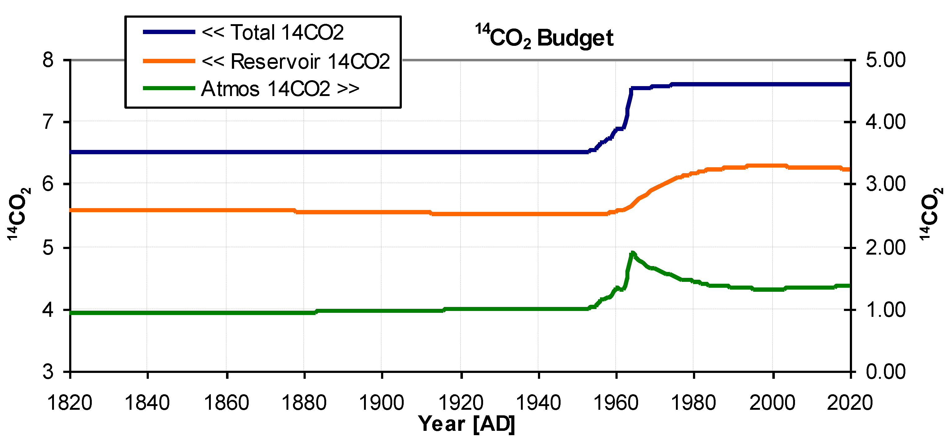
The activity concentration of ¹⁴C, which is its absolute amount rather than its ratio with C, is displayed in Figure 6. The graph shows how the activity concentration of ¹⁴C in the atmosphere and the reservoir changes over time. The total amount of ¹⁴C in the system is represented by the blue curve, while that in the atmosphere is shown in green. In 1960, atmospheric nuclear weapons testing caused a sudden step increase in the amount of ¹⁴C. The atmospheric activity concentration shows the bomb pulse decaying to a minimum around 2000[AD] but then rising slightly again, this has been experimentally determined by Svetlik (2010). Some authors (e.g. Levin et al. 2010) have suggested ¹⁴C industrial pollution may be a partial cause of the increase. However, this study accurately reproduces the ¹⁴C curve without such a requirement. In this study, the increase in activity concentration can be attributed to ¹⁴CO₂ re-emerging from the mixing reservoir, while at the same time causing a slight drop in the reservoir level.

Figure 6. ¹⁴CO2 Budget. Model derived absolute ¹⁴CO2 (also known as activity concentration) for the reservoir (orange), the atmosphere (green), and their total (blue) in units relative to the ¹⁴CO2 content of the atmosphere in 1950. The total, being the sum of reservoir plus atmosphere, shows the near step function in ¹⁴CO2 created by nuclear atmospheric weapons testing. After the initial fall of atmospheric content, the small rise since 2000 is confirmed by the results of Svetlik (2010), see text.

Figure 6. ¹⁴CO2 Budget. Model derived absolute ¹⁴CO2 (also known as activity concentration) for the reservoir (orange), the atmosphere (green), and their total (blue) in units relative to the ¹⁴CO2 content of the atmosphere in 1950. The total, being the sum of reservoir plus atmosphere, shows the near step function in ¹⁴CO2 created by nuclear atmospheric weapons testing. After the initial fall of atmospheric content, the small rise since 2000 is confirmed by the results of Svetlik (2010), see text.

4.4. Flux Time Series

The model calculates the mean gross exchange flux in 2019 as 60 GtC yr^-1, these are approximately 27% of the total IPCC figures (IPCC Ed., 2021 Fig 5.12) of 217 GtC yr^-1, and more closely resemble the ocean figures alone of 54 GtC yr-1. Why is there such a discrepancy? We propose here that it is related to the definition of exchange flux. In the real world, if the nett value of a significant two-way exchange flux is zero, it can only have an effect if it has mixed isotopically en route to and from the reservoir. If there is no isotopic mixing, the returned flux is identical to the original absorbed flux both in its bulk and isotopic content; its effect is therefore insignificant. Thus a portion of the exchange flux has no effect. To determine the "effective exchange flux", the model finds the size of the flux which when mixed in both the reservoir and atmosphere, minimises the discrepancy between its computed 13C and 14C curves and the experimentally determined values. This flux is different from the exchange flux of IPCC 2021, which includes cyclical flows of isotopically identical i.e. unmixed gas. This issue also influences the calculation of residence time, which is defined by "atmospheric mass/removal rate", and has been quoted by many in the field (Harvey 2000). The calculation provdes a figure of ~4 years, being obtained by dividing the atmospheric size of 871 GtC by the gross exchange flux of IPCC 2016 i.e. 217 GtC yr^-1. However, using the model-determined exchange flux of 60 GtC yr-1, we obtain 871/60 which yields a residence lifetime of ~14 years, similar to the observed decay of the bomb pulse. Because isotopic mixing occurs more readily within the ocean, it is therefore also unsurprising that the exchange figure from the model more closely resembles the ocean exchange figures rather than the terrestrial portion. See Discussion.

4.5. Influx and Temperature

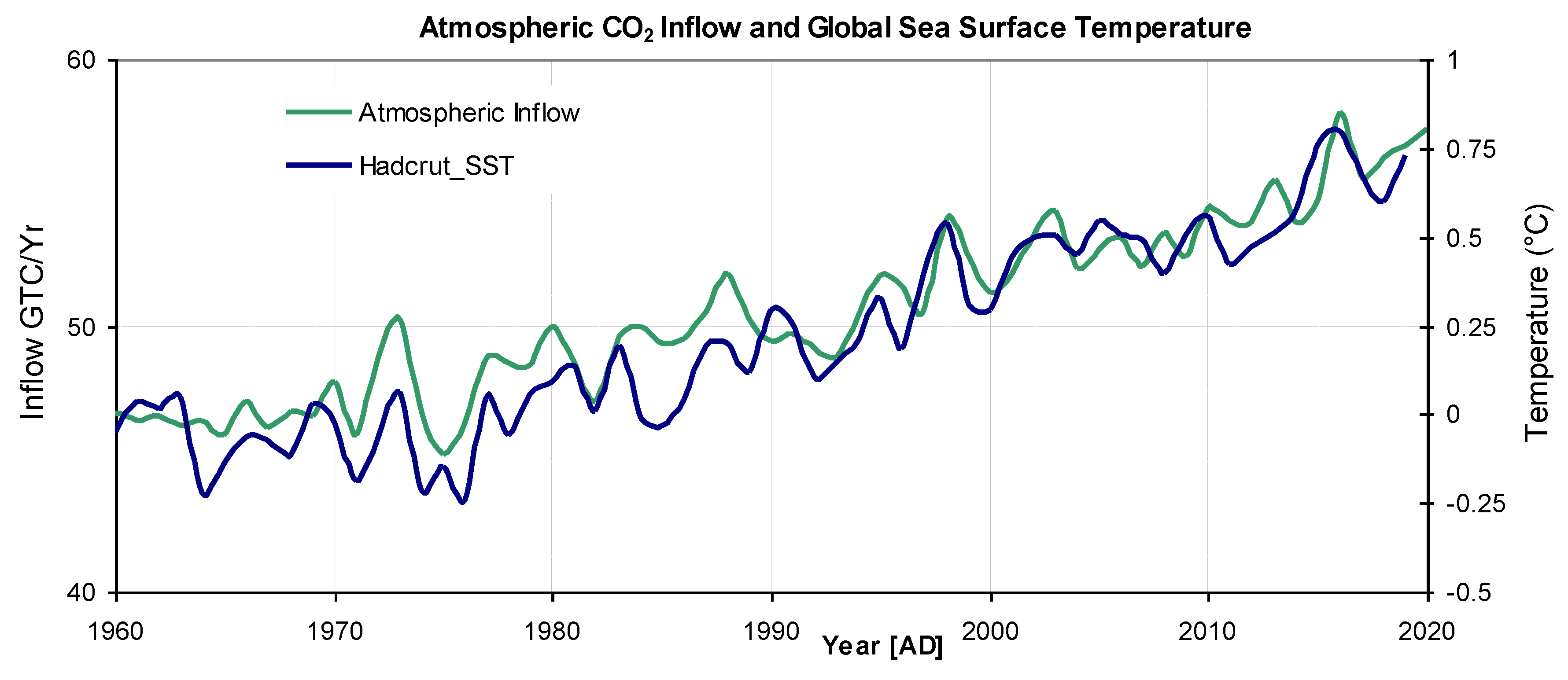
The absolute inflow, computed by the model, is plotted from 1960 to 2020 in Figure 8. Essentially this is an expanded version of the green plot on Figure 7. The same graph also shows global temperature (D7) plotted on a suitable vertical scale, revealing that many of the temperature excursions match CO₂ inflow excursions. The correlation coefficient between the two plots is 0.94. Although correlation cannot be considered as causation, it is difficult to conceive of a mechanism whereby a global temperature change could be influenced by the rate of CO₂ inflow, rather than its absolute atmospheric mixing ratio. An obvious temperature-dependant mechanism for CO₂ gas release in the ocean is the decrease of solubility with temperature. On land the balance between productivity, respiration, decay and temerature has been discussed by Melillo et al. 2011. According to the model, from 1960, annual atmospheric inflow has increased by 12.7 GtC yr^-1 while annual outflow has increased by 13.7 GtC yr^-1.

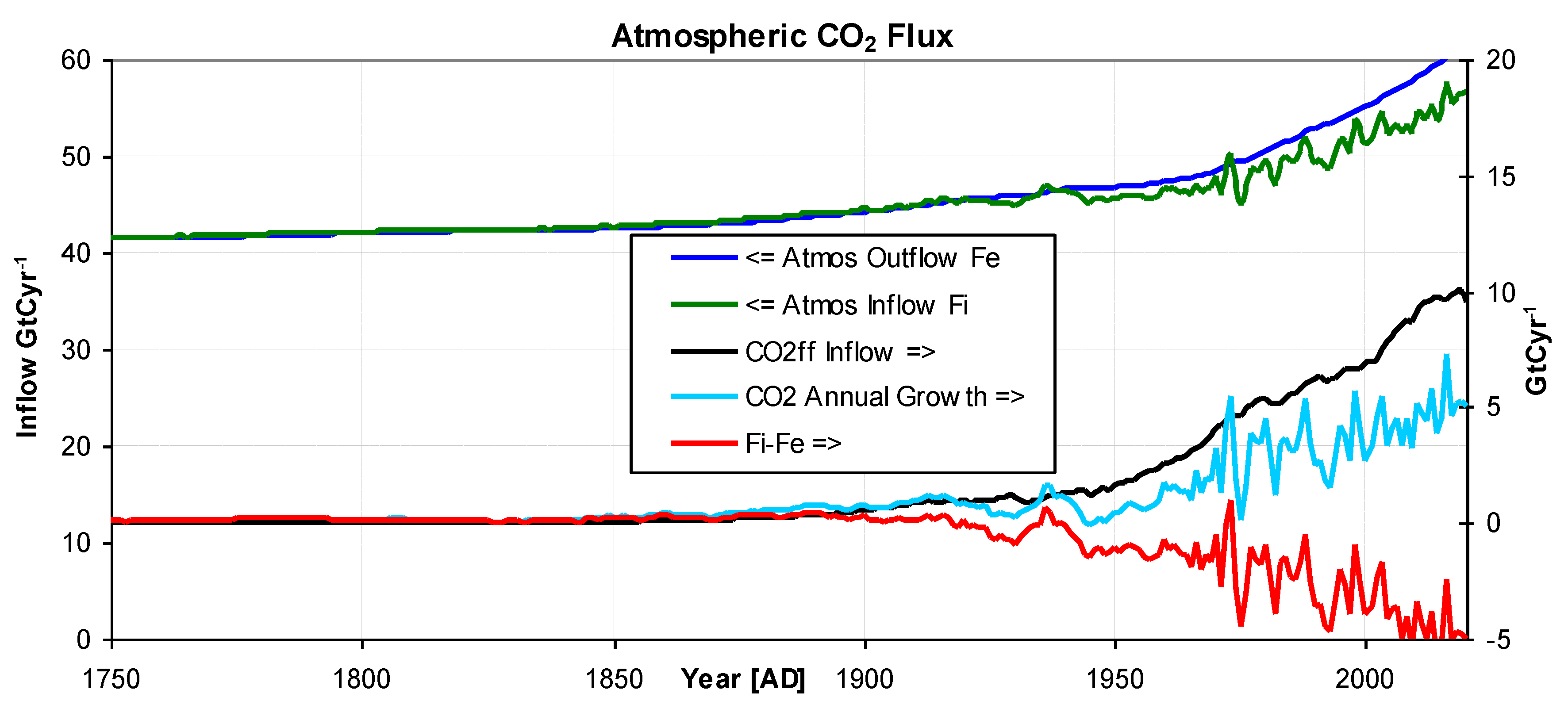
Figure 7. Output from the model showing:- Atmospheric Outflow (blue), Atmospheric Inflow(green), CO2ff Inflow (black) CO2 Atmospheric growth (light blue), and Fi-Fe, (red). The arrow on the legend indicates the relevant axis.

Figure 7. Output from the model showing:- Atmospheric Outflow (blue), Atmospheric Inflow(green), CO2ff Inflow (black) CO2 Atmospheric growth (light blue), and Fi-Fe, (red). The arrow on the legend indicates the relevant axis.

Figure 8. CO₂ inflow (green) and observed global sea-surface temperature (blue) indicating a high degree of correlation of 0.94.

Figure 8. CO₂ inflow (green) and observed global sea-surface temperature (blue) indicating a high degree of correlation of 0.94.

4.6. Cumulative Flux & Levels 1750-2020

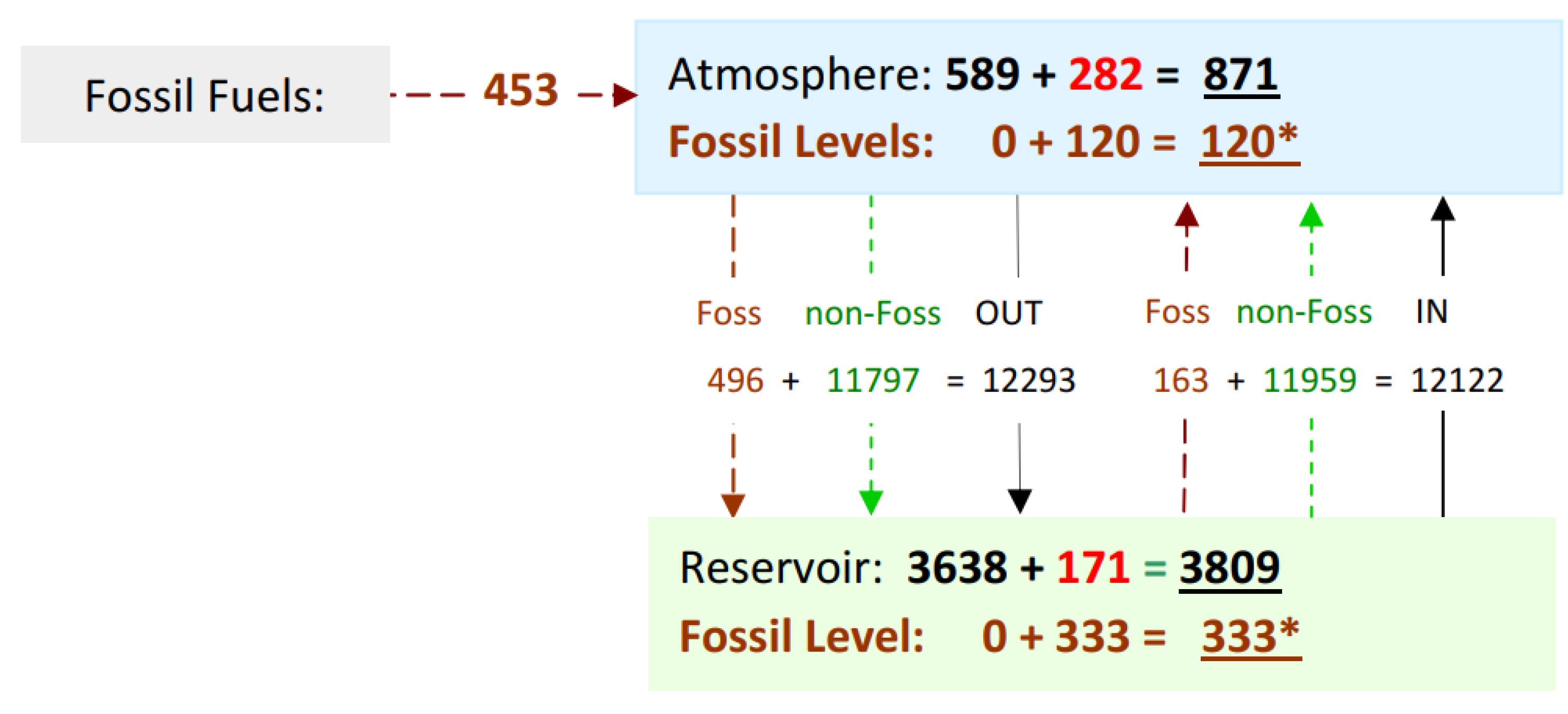
Figure 9 shows the cumulative CO₂ flux and CO₂ levels over a period 270 years, during which, 453 GtC of CO2ff was supplied. Out of this, 282 GtC remains in the atmosphere, while 171 GtC is stored in the reservoir. However, the level of fossil sourced CO₂ increased by 120 GtC in the atmosphere and by 333 GtC in the reservoir, also totalling 453 GtC. Although these figures may seem inconsistent, there is no contradiction. The bulk figures indicate the amount of CO₂ without accounting for its isotopic composition. Fossil level is based upon isotopic content, which depends upon dilution caused by the size of the exchange flux in and out and its source and destination isotopic levels. The relative growth of the atmopsheric CO₂ level since 1750 is 48%. The relative level of fossil fuel emmissions within the atmosphere in 2020, isotpically tracked is 14% (See Rice 2022). In terms of bulk flow, there is a net outflux of 171 GtC from the atmosphere. Figure 7 shows that while both exchange outflow F_e (blue) and inflow F_i (green) are increasing, the outflow has increased more, confirming the nett uptake of CO₂ from the atmosphere by the terrestrial and ocean reservoirs.

5. Discussion

This section provides further evidence challenging the current consensus view regarding CO₂ residence time summarised below. Comparing the oceanic uptake of isotopic CO₂ with the uptake of excess of CO₂ "Siegenthaler and Oeschger (1987) reported that, "The isotopic perturbation vanishes faster than the CO₂ excess". The concept was discussed by Heimann in 1993 "the atmospheric impulse response function of an isotopic perturbation decays much more rapidly than the impulse response function for bulk carbon." Joos in 1994 reported "bomb radiocarbon and anthropogenic CO2 do not behave identically." Houghton 1996, IPCC explained "an atmospheric perturbation in the isotopic ratio disappears much faster than the perturbation in the number of 14C atoms". Tans 2022 explains "The Revelle factor does not apply to isotopic equilibration because a 12CO2 molecule is replaced by a 13CO2 or vice versa. As a result, an isotopic anomaly disappears from the atmosphere more quickly than a total CO2 anomaly." We term here this concept as the "Revelle Bypass" for brevity. The following two sections provide further evidence that bomb radiocarbon and anthropogenic CO₂ do behave similarly within the atmosphere and carbon cycle, supporting the same clear implications derived from the model earlier in this paper, refuting the "Revelle Bypass". This position is not taken lightly, the author believes it is a necessary correction to climate science.

5.1. Isotopic Behaviour

Following Tans' approach (Tans 1994, 2022) we see that a change in atmospheric ¹⁴C concentration can arise in two ways; first from a change in concentration of atmospheric CO₂ even though the ¹⁴C/C ratio remains constant (term A), and second, from a change in ¹⁴C/C ratio while atmospheric CO₂ remains constant (term B). Hence, we have

A    B
F14C = d(CR)/dt = R.dC/dt + C.dR/dt

The author believes Tans' application of this equation to the real world is flawed since Tans only derives the second term. However, the first term is highly significant. In the real world, there is no short-term daily equilibrium in CO₂, since it fluctuates diurnally as the Earth rotates, and the terrestrial /oceanic reservoirs cyclically and continuously exchange large quantities of CO₂. This CO₂ flux brings with it quantities of ¹⁴C and ¹²C, which constitute the first term A. The second term B, is driven by fluctuations in the ¹⁴C/¹²C ratio, such as from decaying vegetable matter which has previously preferential absorbed ¹²C during photosynthesis. We can better estimate the magnitude of the contribution of variations of either term, by dividing both sides by CR giving

A   B
d(CR)/CR = dC/C + dR/R

where R is the isotopic ratio, and C is the amount of bulk carbon. The Revelle factor applies only to term A because it describes a change in bulk carbon; in doing so it applies to the various isotopes equally. A comparison of the local values of the relative sizes of dC/C and dR/R shows term A greatly dominates B. This can be determined by examination of a number of studies (e.g. Bishcof 1960, Dai et al. 2009, Faassen et al, 2022, Leinweber et al., 2009, Olsen et al. 2004, Palonen et al. 2018, Takahashi et al. 2002). The local variation dC/C was estimated from the above references as being of the order of ≈6 ppm/400ppm (≈0.015) per hour, while the variation dR/R for 14C estimated at most as around ≈8‰ (≈0.008) per hour and for 13C ≈ 0.2 ‰ (≈0.0002) per hour. Hence |A| significantly dominates |B|. Therefore, it is irrelevant whether or not B has an ability to bypass carbonate chemistry (i.e. "Revelle Bypass") as claimed by many, since A is the dominant flux, and term A does not have the ability to preferentially bypass seawater chemistry for ¹⁴C. Therefore in practice term A dominates B and both ¹²C and ¹⁴C are equally subject to the effects of seawater carbonate chemistry.

5.2. Airborne Fraction

The airborne fraction is defined as the ratio of atmospheric CO₂ growth to total CO₂ anthropgenic emissions (Friedlingstein 2022). Its relatively stable value of approximately one half was remarked upon by Broeker in 1975. It has been suggested that, since the rise in anthropogenic emissions is approximately exponential, this indicates that absorption of atmospheric CO₂ is governed by an ordinary differential equation (ODE) (Cawley 2011). We provide below the mathematical derivation of airborne fraction, AF from an ODE containing the bulk residence time, t_a and exponential rate-of-rise t_s of anthropogenic emissions, where t_a = 1/a and t_s = 1/s. If fossil fuel emissions increase exponentially, F_a in equation (3) may be replaced with e^st as

dC/dt = -a C + F_i + e^st

(13)

The particular solution for (13) is given by many authors, (Gilbert Strang MIT 2015), and shows the resulting response of CO₂ level (sometime called the "adjustment time") comprises the sum of two time exponentials as

C=(e^st - e^-at)/(s+a) + C₀

(14)

The solution can be verified by substitution of (14) into (13), a step which shows that aC₀ = F_i where C₀ represents the equilibrium value. The instantaneous airborne fraction, being defined as the ratio of the rate of rise of atmospheric CO₂ to the assumed exponentially increasing CO2ff input rate, can be found by dividing by e^st, which, after some manipulation, gives

AF = (dC/dt)/ e^st = s /(s + a) + a e ^-(s+a)t /(s+a) + (F_i(t) - aC₀) e^-st

(15)

The first term represents the value to which the airborne fraction tends; the second represents a transient with negative exponent which rapidly diminishes, and the third represents the out of equilibrium contribution. If F_i is constant it balances the outgoing exchange flux, aC₀ setting the third term to zero and the first term of (15) is the value to which the AF settles. Putting t_a = 1/a and t_s = 1/s we can then write

AF => s/(s+a), a => s(1/AF -1), t_a => t_s /(1/AF - 1)

(16)

The formulae in (16) apply if F_i is constant and if the transient has settled; it also applies to cumulative values. Typical values are AF=0.45, t_s=53 years, (Cawley 2011) giving t_a a value 43 years. The difference in value between this and the bomb pulse decay time (by at least a factor of 3), has been quoted as supporting evidence that the "Revelle Bypass" applies (Harvey 2000). However if F_i is not constant, as is the case in practice, the calculation of AF must use equation (15) rather than the simplified form equation (16), returning a different value. IPCC 2021, in AR6 figure 5.12, shows values of F_i from 1750 rising for land by 25.6 GtC yr^-1 and for ocean 23.0 GtC yr^-1. Similar rising values of F_i are also shown by the model presented in this study, which reports its rise from 41.5 GtC yr^-1 to 56.7 GtC yr^-1, see Figure 8. Applying this rising sequence of F_i to equation (13) with a time constant of 14.2 years yields the resulting time-series shown graphically Figure 10 below. Thus the time constant differs significantly from the value of 43 years which was obtained when F_i was incorrectly assumed to be constant. The longer time constant therefore does not indicate that the "Revelle Bypass" applies, but rather indicates it is an incorrect result caused by ignoring the rising value of F_i. The equation was also solved using an exponential fit to the fossil fuel emissions rather than the emissions themselves giving the similar plot shown in green. The similarity of the plots shows there is no need to invoke the "Revelle Bypass" in order to account for differing time constants.

In addition to resolving any inconsistency in the value of the time constant, the rising nature of F_i also resolves the confusion regarding a single CO₂ lifetime. For example, IPCC tabulates CO₂ lifetime as "5 to 200 yr" with note "c" stating "No single lifetime can be defined for CO₂ because of the different rates of uptake by different removal processes" (IPCC Ed., 2001, Table 1 p38). Thus, even though there may be different removal processes, it is entirely possible to determine the system behaviour using a single effective residence time for CO₂.

6. Conclusion

This study describes a new approach to modelling the carbon cycle, which is implemented in a two-box CO₂ absolute flow model.

• The model accurately describes the values of ¹⁴C and δ¹³C over 200 years, yet without assuming that bomb radiocarbon and anthropogenic carbon behave differently.
• The study shows that the claimed "Revelle Bypass" does not occur in practice because bulk exchange flows dominate isotopic ratio flows. In practice, there is therefore no significant difference in the behaviour of different isotopes, apart from fractionation.
• The study applies the airborne fraction to the calculation of residence time, with modifications to consider and include the presence of a temporal variation in bulk CO₂ exchange inflow. This modification yields the same residence time for bulk CO₂ exchange inflow as for the ¹⁴C bomb pulse, showing the "Revelle Bypass" has been the cause of this confusion.
• Furthermore, the study shows that it is possible for there to be a rising influx of CO₂ from the ocean/land reservoir, and at the same time, a net sink of atmospheric CO₂.

The study overturns a key assumption of the carbon cycle, namely that "bomb radiocarbon and anthropogenic CO₂ do not behave identically." (Joos 1994). This has profound implications for our understanding of the exchange flux and climate change.

The model is available on https://geomatix.net/downloads/iso-uptake.htm