
Submitted:
18 January 2023
Posted:
19 January 2023
You are already at the latest version
Abstract
InSAR and associated analytic methods enable relative surface deformation measurements from low Earth orbit with a potential accuracy of centimeters to millimeters. However, assessing the actual accuracy can be quite difficult. The analytic methods are complicated enough that naive analytic error propagation is infeasible, and, in many settings, InSAR practitioners lack sufficient ground truth to assess results. Phase noise due to partial decorrelation from changes in the scattering properties of the ground is a prominent source of accuracy loss. In this paper we present a method to assess the loss of precision due to this component of phase noise. The proposed method consists of generating synthetic data stacks whose statistical properties match those of the actual input SAR data stacks, and then using the synthetic data for an ensemble calculation. The spread of the results of the ensemble calculation indicates the loss of precision. We show examples of the ensemble analysis at a mining operation in South Africa, and demonstrate the ability to estimate the precision of two InSAR deformation retrieval methods on a point-by-point and epoch-by-epoch basis.
Keywords:
InSAR
; deformation
; synthetic data
; ensemble methods
; uncertainty estimate
; time series analysis
1. Introduction
Interferometric Synthetic Aperture Radar (InSAR) enables measurements of surface deformation with a potential accuracy of centimeters to millimeters (Rosen et al. 2000). A complex valued Synthetic Aperture Radar (SAR) image consists of pixels whose phase is determined by the scattering properties on the Earth’s surface and the effective round trip distance between the satellite and the surface. If the scattering properties change minimally, the phase change between corresponding pixels in two co-registered complex SAR images will reflect changes in the effective round trip distance between the satellite and the surface thereby detecting surface displacements in the imaged area. Methods such as the Small Baseline Subset (SBAS) method (Berardino et al. 2002), the Permanent Scatterers (PS) method (Ferretti et al. 2001), and their variants can then be used to extract surface deformation from phase differences in a series of complex SAR images.
There are a number of potential sources of error that InSAR methods must address to extract the most accurate surface deformation. First, the effective round trip distance between the satellite and the surface includes effects from tropospheric moisture and free electrons in the ionosphere (Goldstein 1995; Zebker et al. 1997). Second, successive passes do not revisit the same orbital paths exactly, which can lead to geometrical decorrelation (Rodriguez and Martin 1992; Zebker and Villasenor 1992). Third, the spatial differences in successive orbit passes contribute a component to the interferometric phase that is independent of deformation. Fourth, the desired component of the phase is the round trip distance between the satellite and the ground modulo the wavelength, which is a few centimeters, mapped to , see Goldstein et al. (1988). The process of recovering an “absolute" phase from the observed or “wrapped" phase is called unwrapping, and without additional constraints the problem is ill-posed. Finally, the scattering properties of the ground change with time, resulting in temporal decorrelation and possibly adding an interferometric phase component, see Zebker and Villasenor (1992).
Many of these issues have been addressed, or are understood, to an acceptable degree. Tropospheric moisture and its contribution to phase, known as atmospheric phase screening (APS), have been studied extensively, e.g. Hanssen (2001, Chapter 6), Ferretti et al. (1999, Section 2), Jolivet et al. (2014) and Yu et al. (2018), and a number of methods to address APS, without using external inputs like weather models, have been presented (Murray et al. 2019; Tymofyeyeva and Fialko 2015; Yu et al. 2017). Absent real-time models of tropospheric moisture, one can assume APS varies slowly in space and any spatial variations in APS can be assumed to be uncorrelated between revisits (Zebker et al. 1997). This helps separate a deformation signal that is consistent in time from APS. Ionospheric effects, which tend to be more significant for L-band and longer wavelength systems, have been similarly studied (Chen and Zebker 2013; Fattahi et al. 2017; Liang et al. 2019). Geometrical decorrelation has been largely addressed by better orbit control. The phase change due to variations in successive orbital passes can be estimated with a digital elevation model (DEM) and precise orbit data. Any gross errors in DEMs can be identified because they manifest as a phase contribution that correlates with the component of orbit offsets that is perpendicular to the look direction (Fattahi and Amelung 2013). This effect is sufficiently reliable to use InSAR to generate DEMs (Van Zyl 2001; Zink et al. 2014). Errors in orbit data contribute a phase term that is typically a ramp in space (Hanssen 2001), though due to the precise orbit data of Sentinel-1 (Peter, et al. 2020) and other modern SAR satellites, the impact of orbital errors on InSAR is negligible (Fattahi and Amelung 2014).
Many of these issues have been addressed, or are understood, to an acceptable degree. Tropospheric moisture and its contribution to phase, known as atmospheric phase screening (APS), have been studied extensively, e.g. Hanssen (2001, Chapter 6), Ferretti et al. (1999, Section 2), Jolivet et al. (2014) and Yu et al. (2018), and a number of methods to address APS, without using external inputs like weather models, have been presented (Murray et al. 2019; Tymofyeyeva and Fialko 2015; Yu et al. 2017). Absent real-time models of tropospheric moisture, one can assume APS varies slowly in space and any spatial variations in APS can be assumed to be uncorrelated between revisits (Zebker et al. 1997). This helps separate a deformation signal that is consistent in time from APS. Ionospheric effects, which tend to be more significant for L-band and longer wavelength systems, have been similarly studied (Chen and Zebker 2013; Fattahi et al. 2017; Liang et al. 2019). Geometrical decorrelation has been largely addressed by better orbit control. The phase change due to variations in successive orbital passes can be estimated with a digital elevation model (DEM) and precise orbit data. Any gross errors in DEMs can be identified because they manifest as a phase contribution that correlates with the component of orbit offsets that is perpendicular to the look direction (Fattahi and Amelung 2013). This effect is sufficiently reliable to use InSAR to generate DEMs (Van Zyl 2001; Zink et al. 2014). Errors in orbit data contribute a phase term that is typically a ramp in space (Hanssen 2001), though due to the precise orbit data of Sentinel-1 (Peter, et al. 2020) and other modern SAR satellites, the impact of orbital errors on InSAR is negligible (Fattahi and Amelung 2014).
Studies of the phase contribution due to changes in scattering properties have largely focused on how to select “good" pixels to include in an InSAR analysis, e.g. Ferretti et al. (2001). These “good" pixels are assumed to have consistent scattering properties. The inability to separate the phase due to scattering process from systematic phase contributions such as orbit variation and APS can be dealt with in several ways. In Ferretti et al. (2001) the authors present an elegant argument relating phase noise to temporal variations in amplitude, which is not affected by APS or orbit variation. This allows one to identify likely permanent scatterers (PS), i.e. pixels where scattering is dominated by a single stable feature. These PS pixels are included in the InSAR analysis. The drawback to using amplitude alone is that it often selects too few pixels outside of urban areas. Consequently, the method presented in Ferretti et al. (2001) includes additional steps to incorporate more pixels whose phases are consistent with these initial PS pixels, but may not have the desired amplitude statistics, allowing the inclusion of more pixels.
Alternatively, because many pervasive phase contributions vary slowly in space, e.g. APS and orbit variations, one can choose a spatial window to determine if the phase changes are at least consistent within that spatial window. At the simplest level one can estimate the interferometric phase difference between two SAR collections as shown in Eqs. 1.13 and 1.14 in Ferretti et al. (2007a). Here one approximates the expectation value of the phase change for a pixel (Eq. 1.13) by assuming the statistics are sufficiently uniform within the averaging window (Eq. 1.14). There are more sophisticated methods that incorporate a stack of co-registered complex SAR images to estimate a consistent time series for the wrapped phase, e.g. Ansari et al. (2018),Guarnieri and Tebaldini (2008). We refer to phase quality between two SAR collections as coherence, and the phase quality for a stack of (more than two) SAR collections temporal coherence. These methods to estimate the quality of interferometric phase, and, in the cases of Ferretti et al. (2007a, Eq. 1.14), Guarnieri and Tebaldini (2008), and Ansari et al. (2018), the phase itself, are based on the idea that phase noise should be considered as a statistical process and these methods can estimate the parameters of that process.
These coherence estimation methods can also be used to estimate uncertainty in phase (Bamler and Just 1993; Jong-Sen Lee et al. 1994; Zheng et al. 2021; Zwieback et al. 2016, Figure 2 and Figure 3). One could assume that uncertainty in the wrapped phase is the same as the uncertainty in the unwrapped phase, and then accumulate uncertainty according to the chosen interferogram network. While this approach can give a rough approximation, there are two shortcomings worth noting. First, unwrapping is necessarily non-linear, and the uncertainty in the unwrapped phase will likely not be the same as the uncertainty in the wrapped phase. As an aside, it is the authors’ experience that the iterative and conditional logic in unwrapping schemes makes a naïve error propagation infeasible. Second, the historical uncertainty is often correlated in a manner that cannot be captured by a single number such as temporal coherence, or even by coherence between, say, successive SAR scenes. For example, coherence between fall and spring SAR scenes may be high, while snow causes scene-to-scene coherence involving scenes collected in winter months to be low. Indeed, phase-linking InSAR methods (Ansari et al. 2018; Guarnieri and Tebaldini 2008) use a sample correlation matrix (SCM) to reconstruct a consistent wrapped phase from all non-redundant interferometric pairs. This suggests that, if one wants to assess the performance of a deformation retrieval method using synthetic data, those synthetic data should reflect correlations in the uncertainties present in the actual data.
This current work proposes a novel method to estimate uncertainty, more specifically precision, in deformation results based on uncertainty in phase on a point-by-point and epoch-by-epoch basis. The method is described in detail in Section 3. The two main ideas behind this method are 1) creating synthetic data whose phase statistics match the statistics of the input data, then 2) estimating the precision based on the standard deviation of an ensemble calculation using these synthetic data. This uncertainty estimation method can then assess a deformation retrieval method by measuring the spread in results in the ensemble of deformation results retrieved, and can allow the estimation of uncertainty. The inputs to this uncertainty estimation method are the co-registered complex SAR images, relevant metadata, e.g. orbit state vectors, orbit collection times, and, if applicable, Doppler centroids, and finally the InSAR deformation retrieval method itself.
We demonstrate this with an example from a mining site in South Africa in Section 4.
2. Background
Previous studies have attempted to assess the accuracy of InSAR derived deformation using GPS/GNSS data, e.g. Armaş et al. (2016),Ferretti et al. (2007b),Jiang and Lohman (2021),Lee et al. (2005),Zebker (2021), leveling measurements, e.g. Luo et al. (2017),Marinkovic et al. (2007),Yang et al. (2016), or indirect methods such as water level, e.g. Lu and Kwoun (2008),Wdowinski et al. (2004) or precipitation, e.g. Palomino-Ángel et al. (2022). However, some of these methods cannot provide a direct comparison to deformation signals and therefore make it difficult to estimate accuracy or precision, and the uncertainty of other methods such as GPS/GNSS and leveling data is comparable if not greater than what is anticipated for InSAR measurements (You 2006). Further, these sources of validation are often temporally or spatially sparse, which does not allow one to estimate the accuracy of all points or epochs used in the InSAR surface deformation measurement and limits the ability to detect where the recovered deformation is most reliable and where it may be less so.
Synthetic data have been used as another way to investigate the accuracy of InSAR analyses, especially with the emergence of inexpensive computing, and are often used in the context of training or validating machine learning models, e.g. Anantrasirichai et al. (2019); Brengman and Barnhart (2021); Lee et al. (2012); Rouet-Leduc et al. (2021); Sica et al. (2020) or to study specific geologic or meteorologic phenomena, e.g. Biggs et al. (2006); Scott and Lohman (2016); Zhang et al. (2021). The main value in using synthetic data in this way is it allows one to estimate how well an input deformation signal can be recovered by a particular deformation retrieval method. This is particularly enticing when no ground truth exists. However, these approaches often use simplified deformation signals and randomly generated noise statistics (Biggs et al. 2006; Rouet-Leduc et al. 2021) or refrain from adding certain noise components all together (Anantrasirichai et al. 2019; Scott and Lohman 2016; Zhang et al. 2021), or they focus on a particular synthetic source (Yunjun et al. 2019) and typically do not explore the potential spread of results for different iterations of randomly generated noise, like the method presented here.
Zheng et al. (2021) presented a detailed model for phase covariance statistics of InSAR stacks and extensively compared it against previously published models (Agram and Simons 2015; Hanssen 2001; Samiei-Esfahany and Hanssen 2017) for certain types of temporal decorrelation characteristics. The “Hanssen model" (Hanssen 2001) was identified as overly optimistic due to assumption of noise terms being uncorrelated between interferograms and the models from Agram and Simons (2015) and Zheng et al. (2021) assume unwrapped interferograms as a starting point, making them computationally intractable for full resolution analysis and infrastructure monitoring applications. These phase covariance models derive theoretical bounds on InSAR time-series uncertainties but do not include mechanisms to assess the impact of individual processing steps or specific implementations of processing steps.
The method presented here builds on the suggestion from Agram and Simons (2015) to consider the neighborhood statistics of each pixel in the temporal domain independently for computational tractability. The approach used to simulate temporal history is very similar to the Monte-Carlo approach presented in Samiei-Esfahany and Hanssen (2017), but has been modified to preserve any systematic per-acquisition phase terms.
3. Method
3.1. Overview
Let N denote the number of complex SAR scenes. We choose a kernel k in the spatial domain and compute the Sample Correlation Matrix (SCM) for each pixel. Recall the entry for the SCM (associated with time epochs r and c) corresponding to pixel i is
where
- is the co-registered complex SAR data at epoch a for a neighborhood of pixel b,
- is the inner product generated by integrating the convolution of the product with the (positive definite) kernel k and
- is the induced norm, i.e. .
To generate sample data for pixel i, we notionally draw from where Z is a random column-vector variable of N i.i.d. entries each drawn from the complex normal distribution . We let
which we treat as the synthetic phase. The synthetic data for pixel i is then the Hadamard, or element-wise, product of and the amplitude vector of the input SAR data at pixel i.
In addition to stacks of co-registered complex SAR scenes, InSAR analysis pipelines require a number of ancillary data such as orbit data and collection dates. We use these ancillary data from the input stack. With this, we can create an ensemble of synthetic data that have the same form as the input data, and any InSAR analytic pipeline can run on both real and synthetic data without change.
Running an InSAR analysis pipeline on an ensemble of such stacks generates a range of deformation results, which helps assess the likely loss of precision, or uncertainty, due to decorrelation, and provides an estimate of precision per pixel and epoch.
3.2. Properties
There are a number properties of this method worth discussing.
The SCM may not be positive semi-definite. Since the SCM is Hermitian, we compute using an eigenvalue decomposition, taking the square roots of the eigenvalues. If we encounter any negative eigenvalues, we set them to zero and proceed.
The phase of the SCM is reflected in the synthetic data. To see this we consider the case of the SCM for a pixel for two epochs. The SCM will have the following form
where the modulus of z is the coherence and the phase of z is the estimated interferometric phase, both of which will depend on our choice of kernel. The eigenvalues and corresponding eigenvectors are , and , , where is the phase of z, i.e. . We can compute the square root of the SCM as
where
- and
- .
- For two i.i.d. random complex Gaussian variables and , we can compute the synthetic phase at the two epochs as
The phase of the SCM will capture contributions whose length scales exceed the width of k (Guarnieri and Tebaldini 2007) – typically APS, deformation and gross DEM errors. Since the synthetic data is derived from the SCM for the real data, and one should not add these phase contributions via additional simulated data.
We are using the SCM as a covariance matrix. It is natural to consider using the covariance matrix itself, which will only fail to be Hermitian positive semi-definite in the case of round-off error. The covariance matrix would be appropriate if we were attempting to estimate the uncertainty in, and create synthetic versions of, both the amplitude and phase by using a windowed average specified by k. Our goal, however, is to create synthetic data that allows us to estimate the uncertainty in phase estimations obtained by spatial averaging.1.
One must choose k. The choice of k impacts the effective resolution of the synthetic data. One should choose k large enough to capture the uncertainty, but small enough to resolve the features of interest. In practice one can choose k so that statistics like coherence or the SCM for the synthetic data match the same statistics of the real data as closely as possible. Since we are comparing deformation at a mining site in this example, we have chosen a kernel k that is suitable for the desired resolution for infrastructure monitoring.
The InSAR method to be assessed will also use a kernel to estimate phase from input SAR data. The choice of this kernel is governed by similar constraints, i.e. the kernel should capture the phase statistics sufficiently and the kernel should resolve desired features. Since the kernel k used to generate the synthetic data determines the effective resolution of the synthetic data, we always choose k to be no larger than the kernel used by the InSAR method’s phase estimation.
The synthetic data this method produces are only appropriate for kernel-based phase estimation. This process of generating synthetic data assumes that phase statistics are nearly uniform on a small scale, and that the kernel k can recover these phase statistics.
This assumption does not hold for a single permanent scatterer surrounded by noisy pixels. Consequently, if one uses amplitude dispersion to detect PSs within a noisy surrounding environment, these synthetic data will not represent the uncertainty in the phase recovered from pixels selected by amplitude dispersion. The method we propose here will construct synthetic data using the statistics from a windowed average, the synthetic version of a single PS surrounded by noisy pixels will reflect the entire neighborhood of that PS, and will not capture the quality of that single pixel on its own. Note that, because the synthetic data use the original amplitudes, the amplitude dispersion calculation will agree exactly for both synthetic and real data, while the synthetic phase for the pixel will likely be less reliable than the corresponding real phase.
One can create synthetic data for single pixels, essentially following Ferretti et al. (2001). One creates a Rice distribution that matches the observed amplitude dispersion, selects the phase from the samples and pairs them with the input amplitude. While substantially simpler than our method based on the SCM, it suffers the drawback that the phase statistics are assumed to be fixed in time. In this case, e.g., seasonal noise will not be captured. Further, such a method will, without additional inputs, produce synthetic data with mean zero phase.
For reasons discussed in Section 5, one may want to further restrict the deformation retrieval methods evaluated to those that use the SCM to estimate a consistent interferometric phase.
The ensemble calculations will likely not all choose the same set of points. Deformation retrieval methods have a pixel selection step based phase statistics. These statistics for the synthetic data are close to, but do not match exactly, the statistics for the real data. For this reason, when assessing the spread in deformation results for a test point relative to a reference point, only the ensemble instances that selected both the test and reference points need to be included.
3.3. Implementation
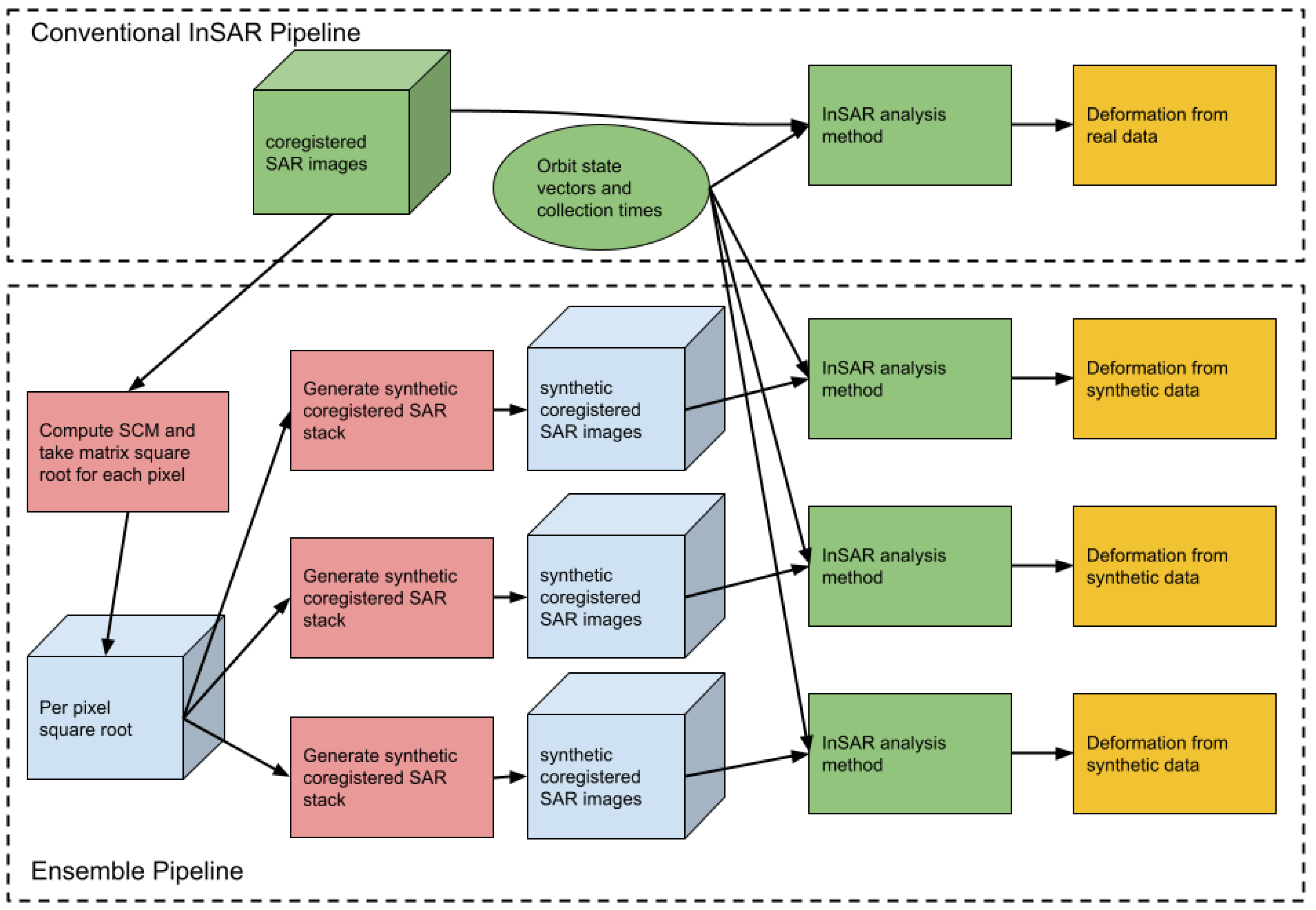
Figure 2 depicts our ensemble method. The inputs are shown in green and are a stack of co-registered complex SAR images, associated metadata, and the InSAR deformation retrieval method to assess. The constraints on the input are that the complex SAR stack needs to be indexable by number of pixel rows by number of pixel columns by number of epochs. The metadata, typically orbit state vectors and collection times need to be in a format that the InSAR method can read. These metadata are not direct inputs to the ensemble calculation.
The core of the method we are presenting is simply a means to take an input stack of SAR data and create synthetic stacks that have similar phase statistics. These synthetic stacks, combined with the original metadata, are then used as input for the InSAR deformation retrieval method being assessed.
There are several computational costs. The first is computing the matrix square root of the SCM for each pixel. We partition the pixels into tiles and dispatch the tiles over a group of virtual central processing units (vCPUs). The resulting per-pixel square root is written to storage so that it can be re-used. The second is forming the synthetic stacks. One creates a vector of i.i.d entries whose length is the number of epochs. One then performs a complex matrix-vector multiply per pixel, and normalizes the recovered phase. The phase is then paired with the original amplitudes. This step is comparatively inexpensive. The last step is running the InSAR deformation retrieval method. We run thirty instances on ensemble data and one on real data, leading to a computational cost that is thirty-one times the cost of a single InSAR analysis.
Figure 2.
A depiction of the method with the inputs in green, the ensemble pipeline computational steps in red, and the outputs in yellow. Pale blue indicates intermediate data. In this image we show three InSAR analyses of synthetic data, in practice we use thirty.
Figure 2.
A depiction of the method with the inputs in green, the ensemble pipeline computational steps in red, and the outputs in yellow. Pale blue indicates intermediate data. In this image we show three InSAR analyses of synthetic data, in practice we use thirty.
In Section 4 and Section 5 we present specific costs for compute and storage, but there are some trends worth noting. First, the matrix square root we use is based on an eigenvalue decomposition and computational grows as where N is the number of epochs. The code to generate an ensemble of synthetic stacks after this step is effectively linear 2 in the number of pixels and in the size of the ensemble, we use thirty synthetic stacks. The remaining cost is in running repeated InSAR analyses. This last item is the most expensive part of the process.
4. Example
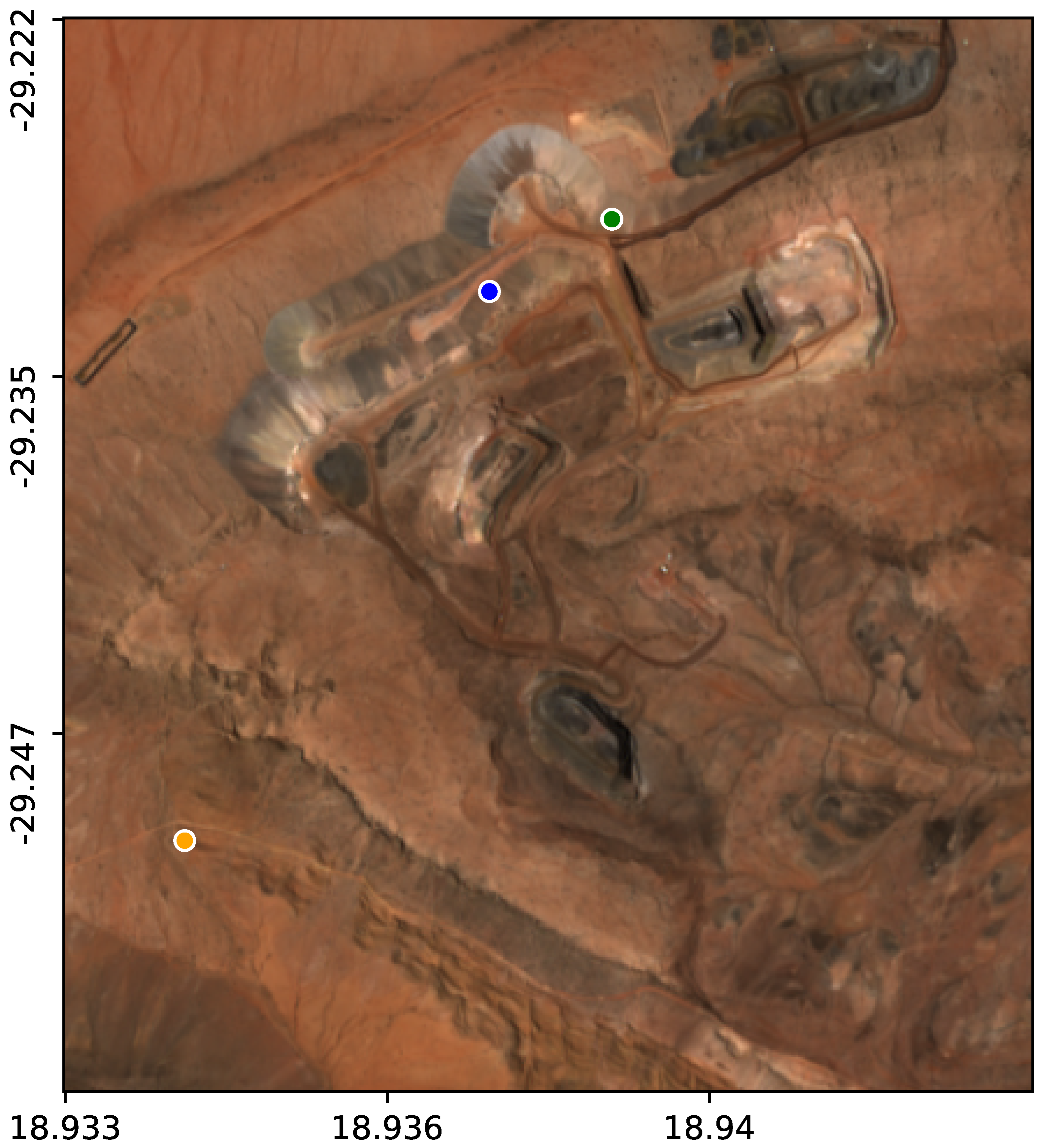
We demonstrate our uncertainty assessment on two InSAR deformation retrieval methods applied to an area in South Africa, shown in Figure 3. Both deformation retrieval methods take as input a stack of 31 images collected by Sentinel-1 track 131 between November of 2019 and November of 2020, as well as ancillary data such as orbit parameters. The images were co-registered to a Universal Transverse Mercator (UTM) coordinate system with resolution of 2.5m East-West by 10m North-South. We chose the anisotropic resolution of the UTM grid to approximate the anisotropy of range and azimuth resolutions in a Sentinel-1 IW-TOPS mode collection.
Figure 3.
Our area of interest with the reference point (orange) and test points (green and blue). Imagery is sourced from Sentinel-2.
Figure 3.
Our area of interest with the reference point (orange) and test points (green and blue). Imagery is sourced from Sentinel-2.
Our uncertainty assessment begins by following the method described in Section 3.1 to generate stacks of synthetic data whose phase statistics match, as best as possible, those of the original, real, input stack. The top of Figure 7 shows the kernel used to form the SCM referenced in Section 3.1. Figure 4 compares coherence between two scenes separated by roughly 120 days for real data and synthetic data. The synthetic data has slightly lower coherence. Figure 5 compares the absolute value of the SCM for the orange, blue and green points shown in Figure 3. As with coherence, the absolute value of the SCM entries for the synthetic data are, on average, slightly lower than their counterparts derived from real data. This is made clear when we look at the joint distributions for real and synthetic data for the modulus and phase of the SCMs as shown in Figure 6.
There are several notable features in Figure 6. First, for real coherence above 0.1, the coherence of the synthetic data is lower than the coherence of the real data. The largest difference between the coherence of real and synthetic data occurs roughly when the coherence of the real data is . At this point the coherence of the synthetic data has a mean of . Second, when the real coherence is below roughly 0.05, the mean of the coherence of the synthetic data is higher than that of the real data. The question of estimating low coherence has been considered in e.g, Zebker and Chen (2005), and new methods have been proposed to improve the resiliency of phase linking to biases in the SCM magnitudes (Zwieback and Meyer 2022). In this case, the same coherence estimation kernel was used for both the real and synthetic data, and we believe that the discrepancy is essentially due to the difference between the mean of a Gaussian distribution and the mean of the absolute value of the Gaussian distribution when the mean approaches zero.
There are two kernels used by this method, both are shown in Figure 7. The first kernel is used to form the SCM that is then used to generate the synthetic data. The second kernel is used to form the SCM used by the InSAR analysis. As noted in Section 3 the first kernel is smaller than the second and was chosen to establish agreement between the derived statistics. Note that the kernels are anisotropic to match the 2.5m East by 10m North sampling of the input complex SAR data. If mapped to geographic coordinates, the kernels would have the same extent in the and East and North directions.
The first of the two deformation retrieval methods, which we call Method 1, begins by using a variant of the recursive phase estimation method described in Ansari et al. (2018). The phase estimation method in Ansari et al. (2018) splits the epochs into smaller groups of epochs, e.g. a stack of 30 epochs may be split into three groups, or mini-stacks, of ten consecutive epochs. The method presents an iterative scheme to estimate a consistent phase within each mini-stack. Mini-stacks are connected by applying the same iterative scheme to a stack of residuals for each initial mini-stack. Our method differs in that we have replaced the iterative scheme presented in Ansari et al. (2018) with the method presented in Guarnieri and Tebaldini (2008), which uses a single eigenvalue decomposition of a modified SCM. Pixels are included if the temporal coherence averaged over mini-stacks is greater than 0.6.
We reconstruct point data from link data following the method described in Gonzalez et al. (2011). The first step is to reconstruct point deformation rates and point DEM errors from the link-based differential quantities by minimizing the norm of the link residual. The justification presented in Gonzalez et al. (2011) for this norm is that the (as opposed to the ) residual is more likely to identify links that are outliers and should be discarded.
After rejecting links, either due to poor results from Lambda or due to a high residual, the initial set of points may no longer be connected. The method then identifies the remaining connected components and discards components that have four points or fewer. Multiple links are then added between pairs of neighboring connected components to ensure the entire graph is connected. We create an interferogram network using a minimum spanning tree of the SAR collections plotted in temporal-perpendicular baseline space. Each interferogram is unwrapped by minimization of the phase gradients from the Lambda estimator. With this we can recover time resolved deformation.
The second method (Method 2) begins with the pixel selection and phase estimation method described in Guarnieri and Tebaldini (2008). Following Pepe and Lanari (2006), we use a minimum cost-flow method to establish consistent link values for a Delaunay triangulation of temporal-perpendicular baseline-space, and then use a second minimum cost-flow solve on the Delaunay triangulation of the selected pixels to recover unwrapped phase per point.
At the conclusion of both methods we attempt to remove unwrapping errors as follows: For each link in the Delaunay triangulation of selected pixels, we look at the time series of unwrapped phase difference across the link. If a difference has an absolute value that is more than and is also more then from the mean of differences, we adjust the difference by subtracting or adding 2. These updates to the unwrapped phase difference across the link are converted into updates to unwrapped point data via a least-squares solve. No effort has been made to identify and remove APS, nor have we applied any temporal smoothing.
We have run each method on the real data, and on an ensemble of thirty synthetic stacks of data. These sixty-two deformation retrieval computations were performed on the Descartes Labs Platform (Beneke et al. 2017). Figure 8 shows the recovered cumulative deformation of the real data for the two methods and the standard deviation of the ensemble of cumulative deformation.
Figure 9 and Figure 10 show the time resolved deformation histories at the green and blue points referenced to the orange point for the two methods. We are primarily interested in the spread in the deformation histories recovered from synthetic data. We consider the spread an indicator of the method’s sensitivity to phase noise at those points.
4.1. Costs
Table 1 presents the scale and computational and storage costs for this example. The costs are broken down as follows:
- Co-registration: We perform co-registration for a single scene on a single vCPU. Each scene is stored as a GeoTIFF. The details of the co-registration process can be found in Agram et al. (2022). Note that this cost will be present for any InSAR pipeline, and this cost is shared between the two InSAR methods being assessed, since these data are reused.
- Synthetic Data Generation: This requires reading the co-registered data, forming the sample correlation matrix for every pixel, and computing an eigenvalue decomposition to allow a matrix square root. In addition the matrix square roots need to be stored for the duration of the ensemble calculation, at which point these matrices can be deleted. These tasks are run in a cloud-based, scalable compute environment. Note that we could have reused the matrix square root computations between these two methods, but did not. Compute times for the matrix square-root operation, 0.34 and 0.27 vCPU hours, reflect variations in runtime due to task scheduling on preemptible vCPUs.
- InSAR analyses: This is the most computationally expensive aspect since it requires running the InSAR analysis on real data and then the same analysis on each instance of the synthetic data. Finally the results for each analysis need to be stored. These tasks are also run in a cloud-based, scalable compute environment.
- Dispatch: In our implementation we have a single vCPU that is used to dispatch and monitor tasks associated with the processing. The vCPU time varies depending on how quickly the tasks go through the schedulers queue.
5. Discussion
Figure 9 shows less than 2mm of variability in the ensemble cumulative deformation for Method 1. We take this as an indication that the deformation at the green point referenced to the orange point, as recovered by Method 1, is not particularly sensitive to the simulated phase noise. The same figure shows 5mm of variability in the ensemble cumulative deformation for Method 2, which suggests this method is somewhat sensitive to the phase noise. Figure 10 shows roughly 30mm of variability for Method 1 in the ensemble cumulative deformation for the deformation at the blue point referenced to the orange point. We infer that, for this pair of points and this method, there is substantial sensitivity to phase noise. This same figure shows a variability in Method 2 of about 5mm in the ensemble cumulative deformation, suggesting that the deformation recovered by Method 2 is modestly sensitive to simulated phase noise.
The main benefit in using the presented approach is that, because this method estimates uncertainty point-by-point and epoch-by-epoch, one can filter points based on the magnitude of their estimated uncertainty, which allows confidence that the extracted deformation at the remaining points is relatively insensitive to phase noise and is likely more reliable. Method 1’s sensitivity to simulated phase noise when recovering deformation is quite low for the green point and much higher for the blue point. This could be attributed to the fast decorrelation at the blue point, which is shown by drop in coherence with distance from the SCM diagonal in the middle images in Figure 5 as compared to the decorrelation rate one could infer for the green point shown in the right images of Figure 5. However, if this is the case, why did we not see a similar drop in performance for Method 2?
Looking at the points that were selected by Method 1 can give some insight into why Method 1 had higher variations than Method 2 for the blue test point. Figure 11 shows the blue and green test points plotted on top of the ensemble standard deviation for the cumulative deformation recovered by Method 1. The blue test point is located in a group of points showing a standard deviation of at least 20mm (in yellow). These points are closer to each other than they are to the rest of the point cloud. This cluster of points may have become disconnected during the link-rejection steps of Method 1, and are connected to the rest of the point cloud by links that were added to ensure the point cloud stays connected, but which may not pass the link quality checks. In contrast Figure 8 shows that for Method 2 both the green and blue test points are not in a cluster that is separated from the larger point cloud.
Regardless of the cause, InSAR results can vary based on the deformation retrieval method, e.g. (Hu et al. 2016; Osmanoğlu et al. 2016; Parizzi and Brcic 2010; Yang et al. 2016, Figure 8 and Figure 9), and even individual methods likely have accuracy and uncertainty that varies in space and time. This can make it difficult to determine which points in the results are actually reliable. The primary value of this ensemble method, as shown above, is that it allows us to estimate how sensitive a deformation retrieval method is to phase noise on a pixel-by-pixel and epoch-by-epoch basis, we consider this sensitivity as an indicator of uncertainty.
It is worth noting that low uncertainty, i.e. high precision, is desirable, but is not the same as accuracy. Consider the hypothetical case that all of the ensemble analyses made the same unwrapping error, the resulting uncertainty estimate would be low, i.e. precision is high, but accuracy would be low as well. The authors’ experience with this method is that an unwrapping error manifests as a jump of roughly half a wavelength that is uncharacteristic of the deformation history for that point. When we have seen such cases, we typically see a corresponding spread in deformation results. As an example, the top left panel of Figure 10 shows one of ensemble deformation histories that jumps substantially at the seventh epoch. Almost surely this is in indication of an unwrapping error, but we also see a spread in the ensemble results.
The method to create synthetic data is designed so that SCMs for synthetic data match the corresponding SCMs of the real data. An implication of this is that deformation retrieval methods that estimate consistent interferometric phases from the SCMs may be better assessed by this ensemble method than those deformation retrieval methods that do not. Both method 1 and method 2 considered here have that property. Indeed the phase estimation methods described in Ansari et al. (2018) and Guarnieri and Tebaldini (2008), used by Methods 1 and 2 respectively, ensure interferometric phase closure by construction. In contrast low-bandwidth SBAS methods do not have that property and may suffer from systematic biases (Ansari et al. 2020). There is larger question of understanding how a method is sensitive to statistical properties, not captured by the SCM, of the complex input data.
As we discussed in Section 3, we treat a correlation matrix as a covariance matrix, and take the square root of positive semi-definite approximation of this correlation matrix. These approximations have drawbacks, but result in a computationally tractable method, and Figure 5 and Figure 6 show qualitatively good agreement between the SCMs for real and synthetic data. And the most prominent difference is that synthetic coherence is somewhat lower than real coherence.
The computational and storage costs, aside from generating the synthetic data, require running the entire deformation retrieval process tens of times to generate the actual retrieved deformation and the ensemble analysis, which can each be computationally-expensive, depending on the size and resolution of the area. We also must store each of these results before actually calculating the ensemble mean and standard deviation, which adds additional storage and computation costs. The compute and storage requirements, particularly if one wants to apply this method in multiple cases, makes this ensemble method difficult on a single computer.
Finally, because the standard deviations varies with choice of reference point, there is not a way to compute the standard deviation per pixel and epoch “up front". Instead, when reviewing the results, we have all ensemble results available and re-compute the standard deviations for the test point after changing the spatial reference for all ensemble instances whenever we move the reference point. Although this adds some additional computation and storage costs, it also allows for the flexibility to assess the uncertainty for pairs of reference and test points.
6. Conclusions
We have developed a method for generating synthetic SAR data stacks based on real SAR data stacks. The coherence and estimated phase statistics of the synthetic data appears to match those same properties of the real data. This allows us to perform ensemble studies to assess the sensitivity of particular deformation retrieval method to phase noise. The proposed ensemble analysis can provide a point-by-point, epoch-by-epoch, indication of reliability of the result.
Acknowledgments
The authors would like to thank Mike Warren and Scott Arko for maintaining Descartes Labs Sentinel-1 data pipeline and for helpful discussions relating to InSAR. This work contains modified Copernicus Sentinel data from 2019-2020, and 2022, processed by ESA.
References
- Agram, P.S., Simons, M., 2015. A noise model for insar time series. Journal of Geophysical Research: Solid Earth 120, 2752–2771. [CrossRef]
- Agram, P.S., Warren, M.S., Calef, M.T., Arko, S.A., 2022. An efficient global scale sentinel-1 radar backscatter and interferometric processing system. Remote Sensing 14. URL: https://www.mdpi.com/2072-4292/14/15/3524. [CrossRef]
- Anantrasirichai, N., Biggs, J., Albino, F., Bull, D., 2019. The application of convolutional neural networks to detect slow, sustained deformation in insar time series. Geophysical Research Letters 46, 11850–11858. [CrossRef]
- Ansari, H., De Zan, F., Bamler, R., 2018. Efficient phase estimation for interferogram stacks. IEEE Transactions on Geoscience and Remote Sensing 56, 4109–4125. [CrossRef]
- Ansari, H., De Zan, F., Parizzi, A., 2020. Study of systematic bias in measuring surface deformation with sar interferometry. IEEE Transactions on Geoscience and Remote Sensing 59, 1285–1301. [CrossRef]
- Armaş, I., Gheorghe, M., Lendvai, A.M., Dumitru, P.D., Bădescu, O., Călin, A., 2016. Insar validation based on gnss measurements in bucharest. International Journal of Remote Sensing 37, 5565–5580. [CrossRef]
- Bamler, R., Just, D., 1993. Phase statistics and decorrelation in sar interferograms, in: Proceedings of IGARSS’93-IEEE International Geoscience and Remote Sensing Symposium, IEEE. pp. 980–984.
- Beneke, C.M., Skillman, S., Warren, M.S., Kelton, T., Brumby, S.P., Chartrand, R., Mathis, M., 2017. A platform for scalable satellite and geospatial data analysis, in: AGU Fall Meeting Abstracts, pp. IN32C–04.
- Berardino, P., Fornaro, G., Lanari, R., Sansosti, E., 2002. A new algorithm for surface deformation monitoring based on small baseline differential sar interferograms. IEEE Transactions on Geoscience and Remote Sensing 40, 2375–2383. [CrossRef]
- Biggs, J., Bergman, E., Emmerson, B., Funning, G.J., Jackson, J., Parsons, B., Wright, T.J., 2006. Fault identification for buried strike-slip earthquakes using insar: The 1994 and 2004 al hoceima, morocco earthquakes. Geophysical Journal International 166, 1347–1362. [CrossRef]
- Brengman, C.M., Barnhart, W.D., 2021. Identification of surface deformation in insar using machine learning. Geochemistry, Geophysics, Geosystems 22, e2020GC009204. [CrossRef]
- Chen, A.C., Zebker, H.A., 2013. Reducing ionospheric effects in insar data using accurate coregistration. IEEE transactions on geoscience and remote sensing 52, 60–70. [CrossRef]
- Fattahi, H., Amelung, F., 2013. Dem error correction in insar time series. IEEE Transactions on Geoscience and Remote Sensing 51, 4249–4259. [CrossRef]
- Fattahi, H., Amelung, F., 2014. InSAR uncertainty due to orbital errors. Geophysical Journal International 199, 549–560. [CrossRef]
- Fattahi, H., Simons, M., Agram, P., 2017. Insar time-series estimation of the ionospheric phase delay: An extension of the split range-spectrum technique. IEEE Transactions on Geoscience and Remote Sensing 55, 5984–5996. [CrossRef]
- Ferretti, A., Monti-Guarnieri, A., Prati, C., Rocca, F., 2007a. Part c insar processing: a mathematical approach. InSAR Principles: Guidelines for SAR Interferometry Procs. and Interpretation, K. Fletcher, Ed., ESA Publications: Noordwijk, Netherlands, 3–13.
- Ferretti, A., Prati, C., Rocca, F., 1999. Multibaseline insar dem reconstruction: The wavelet approach. IEEE Transactions on geoscience and remote sensing 37, 705–715. [CrossRef]
- Ferretti, A., Prati, C., Rocca, F., 2001. Permanent scatterers in sar interferometry. IEEE Transactions on Geoscience and Remote Sensing 39, 8–20.
- Ferretti, A., Savio, G., Barzaghi, R., Borghi, A., Musazzi, S., Novali, F., Prati, C., Rocca, F., 2007b. Submillimeter accuracy of insar time series: Experimental validation. IEEE Transactions on Geoscience and Remote Sensing 45, 1142–1153. [CrossRef]
- Goldstein, R., 1995. Atmospheric limitations to repeat-track radar interferometry. Geophysical research letters 22, 2517–2520. [CrossRef]
- Goldstein, R.M., Zebker, H.A., Werner, C.L., 1988. Satellite radar interferometry: Two-dimensional phase unwrapping. Radio science 23, 713–720. [CrossRef]
- Gonzalez, F.R., Bhutani, A., Adam, N., 2011. L1 network inversion for robust outlier rejection in persistent scatterer interferometry, in: 2011 IEEE International Geoscience and Remote Sensing Symposium, IEEE. pp. 75–78. [CrossRef]
- Guarnieri, A.M., Tebaldini, S., 2007. Hybrid cramér–rao bounds for crustal displacement field estimators in sar interferometry. IEEE signal processing letters 14, 1012–1015. [CrossRef]
- Guarnieri, A.M., Tebaldini, S., 2008. On the exploitation of target statistics for sar interferometry applications. IEEE Transactions on Geoscience and Remote Sensing 46, 3436–3443. [CrossRef]
- Hanssen, R.F., 2001. Radar interferometry: data interpretation and error analysis. volume 2. Springer Science & Business Media.
- Hu, J., Ding, X., Li, Z., Zhang, L., Zhu, J., Sun, Q., Gao, G., 2016. Vertical and horizontal displacements of los angeles from insar and gps time series analysis: Resolving tectonic and anthropogenic motions. Journal of Geodynamics 99, 27–38. [CrossRef]
- Jiang, J., Lohman, R.B., 2021. Coherence-guided insar deformation analysis in the presence of ongoing land surface changes in the imperial valley, california. Remote Sensing of Environment 253, 112160. [CrossRef]
- Jolivet, R., Agram, P.S., Lin, N.Y., Simons, M., Doin, M.P., Peltzer, G., Li, Z., 2014. Improving insar geodesy using global atmospheric models. Journal of Geophysical Research: Solid Earth 119, 2324–2341. [CrossRef]
- Jong-Sen Lee, Hoppel, K.W., Mango, S.A., Miller, A.R., 1994. Intensity and phase statistics of multilook polarimetric and interferometric sar imagery. IEEE Transactions on Geoscience and Remote Sensing 32, 1017–1028. [CrossRef]
- Lee, C.W., Lu, Z., Jung, H.S., 2012. Simulation of time-series surface deformation to validate a multi-interferogram insar processing technique. International Journal of Remote Sensing 33, 7075–7087. [CrossRef]
- Lee, I., Chang, H.C., Ge, L., 2005. Gps campaigns for validation of insar derived dems. Journal of Global Positioning Systems 4, 82–87. [CrossRef]
- Liang, C., Agram, P., Simons, M., Fielding, E.J., 2019. Ionospheric correction of insar time series analysis of c-band sentinel-1 tops data. IEEE Transactions on Geoscience and Remote Sensing 57, 6755–6773. [CrossRef]
- Lu, Z., Kwoun, O.i., 2008. Radarsat-1 and ers insar analysis over southeastern coastal louisiana: Implications for mapping water-level changes beneath swamp forests. IEEE Transactions on Geoscience and Remote Sensing 46, 2167–2184. [CrossRef]
- Luo, Q., Zhou, G., Perissin, D., 2017. Monitoring of subsidence along jingjin inter-city railway with high-resolution terrasar-x mt-insar analysis. Remote Sensing 9, 717. [CrossRef]
- Marinkovic, P., Ketelaar, G., van Leijen, F., Hanssen, R., 2007. Insar quality control: Analysis of five years of corner reflector time series, in: Proceedings of Fringe 2007 Workshop (ESA SP-649), Frascati, Italy, p. 30.
- Murray, K.D., Bekaert, D.P., Lohman, R.B., 2019. Tropospheric corrections for insar: Statistical assessments and applications to the central united states and mexico. Remote Sensing of Environment 232, 111326. [CrossRef]
- nal Osmanoğlu, B., Sunar, F., Wdowinski, S., Cabral-Cano, E., 2016. Time series analysis of insar data: Methods and trends. ISPRS Journal of Photogrammetry and Remote Sensing 115, 90–102. [CrossRef]
- Palomino-Ángel, S., Vázquez, R., Hampel, H., Anaya, J., Mosquera, P., Lyon, S.W., Jaramillo, F., 2022. Retrieval of simultaneous water-level changes in small lakes with insar. Geophysical Research Letters 49, e2021GL095950. [CrossRef]
- Parizzi, A., Brcic, R., 2010. Adaptive insar stack multilooking exploiting amplitude statistics: A comparison between different techniques and practical results. IEEE Geoscience and Remote Sensing Letters 8, 441–445. [CrossRef]
- Pepe, A., Lanari, R., 2006. On the extension of the minimum cost flow algorithm for phase unwrapping of multitemporal differential sar interferograms. IEEE Transactions on Geoscience and remote sensing 44, 2374–2383. [CrossRef]
- Peter, H., Fernández, J., Féménias, P., 2020. Copernicus Sentinel-1 satellites: sensitivity of antenna offset estimation to orbit and observation modelling. Advances in Geosciences 50, 87–100. [CrossRef]
- Rodriguez, E., Martin, J., 1992. Theory and design of interferometric synthetic aperture radars, in: IEE Proceedings F (Radar and Signal Processing), IET. pp. 147–159. [CrossRef]
- Rosen, P.A., Hensley, S., Joughin, I.R., Li, F.K., Madsen, S.N., Rodriguez, E., Goldstein, R.M., 2000. Synthetic aperture radar interferometry. Proceedings of the IEEE 88, 333–382. [CrossRef]
- Rouet-Leduc, B., Jolivet, R., Dalaison, M., Johnson, P.A., Hulbert, C., 2021. Autonomous extraction of millimeter-scale deformation in insar time series using deep learning. Nature communications 12, 1–11. [CrossRef]
- Samiei-Esfahany, S., Hanssen, R., 2017. On the evaluation of second order phase statistics in sar interferogram stacks. Earth Observation and Geomatics Engineering 1, 1–15. [CrossRef]
- Scott, C.P., Lohman, R.B., 2016. Sensitivity of earthquake source inversions to atmospheric noise and corrections of insar data. Journal of Geophysical Research: Solid Earth 121, 4031–4044. [CrossRef]
- Sica, F., Gobbi, G., Rizzoli, P., Bruzzone, L., 2020. ϕ-net: Deep residual learning for insar parameters estimation. IEEE Transactions on Geoscience and Remote Sensing 59, 3917–3941. [CrossRef]
- Tymofyeyeva, E., Fialko, Y., 2015. Mitigation of atmospheric phase delays in insar data, with application to the eastern california shear zone. Journal of Geophysical Research: Solid Earth 120, 5952–5963. [CrossRef]
- Van Zyl, J.J., 2001. The shuttle radar topography mission (srtm): a breakthrough in remote sensing of topography. Acta Astronautica 48, 559–565. [CrossRef]
- Wdowinski, S., Amelung, F., Miralles-Wilhelm, F., Dixon, T.H., Carande, R., 2004. Space-based measurements of sheet-flow characteristics in the everglades wetland, florida. Geophysical Research Letters 31. [CrossRef]
- Yang, K., Yan, L., Huang, G., Chen, C., Wu, Z., 2016. Monitoring building deformation with insar: Experiments and validation. Sensors 16, 2182. [CrossRef]
- You, R.J., 2006. Local geoid improvement using gps and leveling data: Case study. Journal of surveying engineering 132, 101–107. [CrossRef]
- Yu, C., Li, Z., Penna, N.T., Crippa, P., 2018. Generic atmospheric correction model for interferometric synthetic aperture radar observations. Journal of Geophysical Research: Solid Earth 123, 9202–9222. [CrossRef]
- Yu, C., Penna, N.T., Li, Z., 2017. Generation of real-time mode high-resolution water vapor fields from gps observations. Journal of Geophysical Research: Atmospheres 122, 2008–2025. [CrossRef]
- Yunjun, Z., Fattahi, H., Amelung, F., 2019. Small baseline insar time series analysis: Unwrapping error correction and noise reduction. Computers and Geosciences 133, 104331. [CrossRef]
- Zebker, H., 2021. Accuracy of a model-free algorithm for temporal insar tropospheric correction. Remote Sensing 13, 409. [CrossRef]
- Zebker, H.A., Chen, K., 2005. Accurate estimation of correlation in InSAR observations. IEEE Geoscience and Remote Sensing Letters 2, 124–127. [CrossRef]
- Zebker, H.A., Rosen, P.A., Hensley, S., 1997. Atmospheric effects in interferometric synthetic aperture radar surface deformation and topographic maps. Journal of geophysical research: solid earth 102, 7547–7563. [CrossRef]
- Zebker, H.A., Villasenor, J., 1992. Decorrelation in interferometric radar echoes. IEEE Transactions on geoscience and remote sensing 30, 950–959. [CrossRef]
- Zhang, Y., Shan, X., Gong, W., Zhang, G., 2021. The ambiguous fault geometry derived from insar measurements of buried thrust earthquakes: a synthetic data based study. Geophysical Journal International 225, 1799–1811. [CrossRef]
- Zheng, Y., Zebker, H., Michaelides, R., 2021. A new decorrelation phase covariance model for noise reduction in unwrapped interferometric phase stacks. IEEE Transactions on Geoscience and Remote Sensing 59, 10126–10135. [CrossRef]
- al Zink, M., Bachmann, M., Brautigam, B., Fritz, T., Hajnsek, I., Moreira, A., Wessel, B., Krieger, G., 2014. Tandem-x: The new global dem takes shape. IEEE Geoscience and Remote Sensing Magazine 2, 8–23. [CrossRef]
- Zwieback, S., Meyer, F.J., 2022. Reliable InSAR Phase History Uncertainty Estimates. IEEE Transactions on Geoscience and Remote Sensing 60, 1-9. [CrossRef]
- Zwieback, S., Liu, X., Antonova, S., Heim, B., Bartsch, A., Boike, J., Hajnsek, I., 2016. A statistical test of phase closure to detect influences on dinsar deformation estimates besides displacements and decorrelation noise: Two case studies in high-latitude regions. IEEE Transactions on Geoscience and Remote Sensing 54, 5588–5601. [CrossRef]
| 1 | The authors attempted to use the actual covariance matrix and found that the resulting synthetic data had coherence that was much lower than the coherence of the real data. |
| 2 | There is a matrix-vector multiply whose cost is not linear in N, but in practice this cost is negligible. |
Figure 1.
Numerical experiments showing the standard deviation of the phase of as a function of .
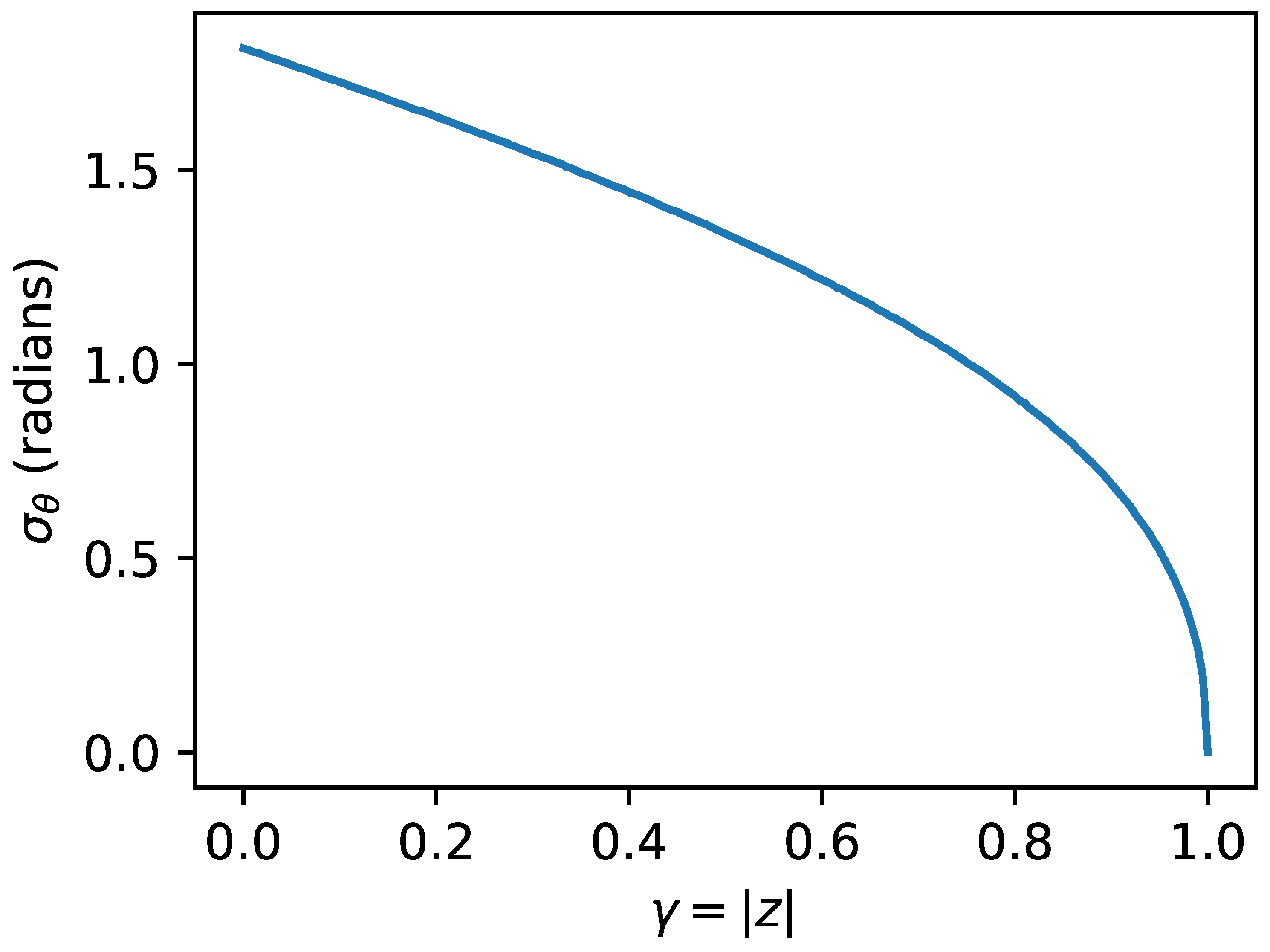
Figure 4.
Coherence between the tenth and twentieth scene, collected on March 4th and July 2nd of 2020 respectively, for real input data (top) and a synthetic stack (bottom).
Figure 4.
Coherence between the tenth and twentieth scene, collected on March 4th and July 2nd of 2020 respectively, for real input data (top) and a synthetic stack (bottom).
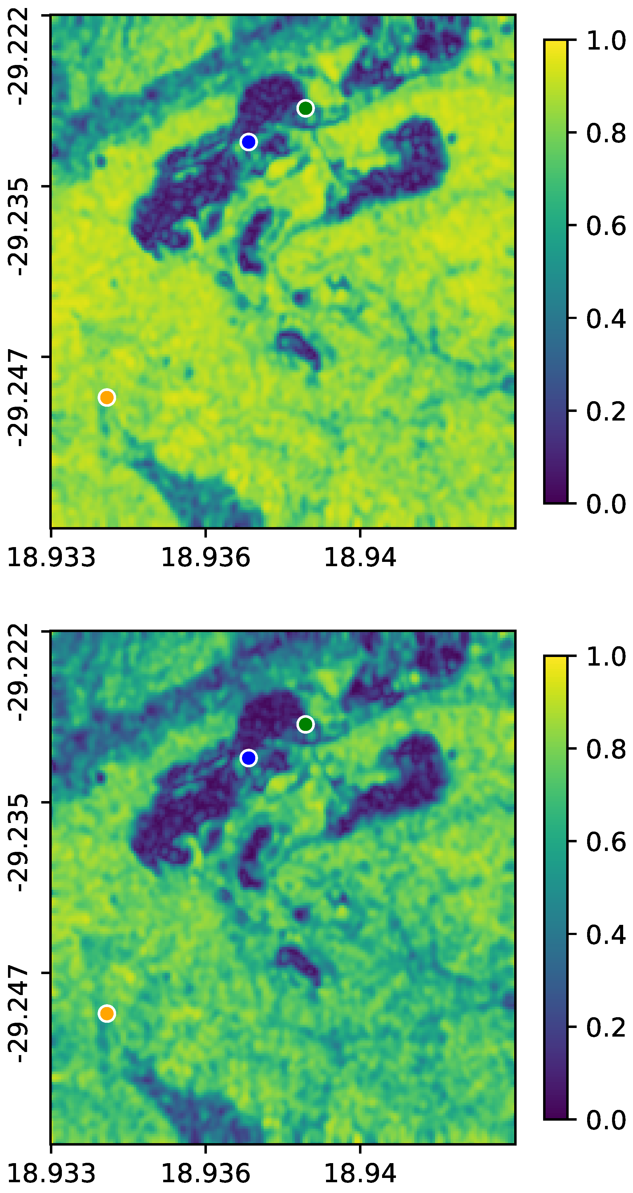
Figure 5.
Absolute value of the sample correlation matrix for the orange (left), blue (middle) and green (right) points for real data (top) and synthetic data (bottom).
Figure 5.
Absolute value of the sample correlation matrix for the orange (left), blue (middle) and green (right) points for real data (top) and synthetic data (bottom).
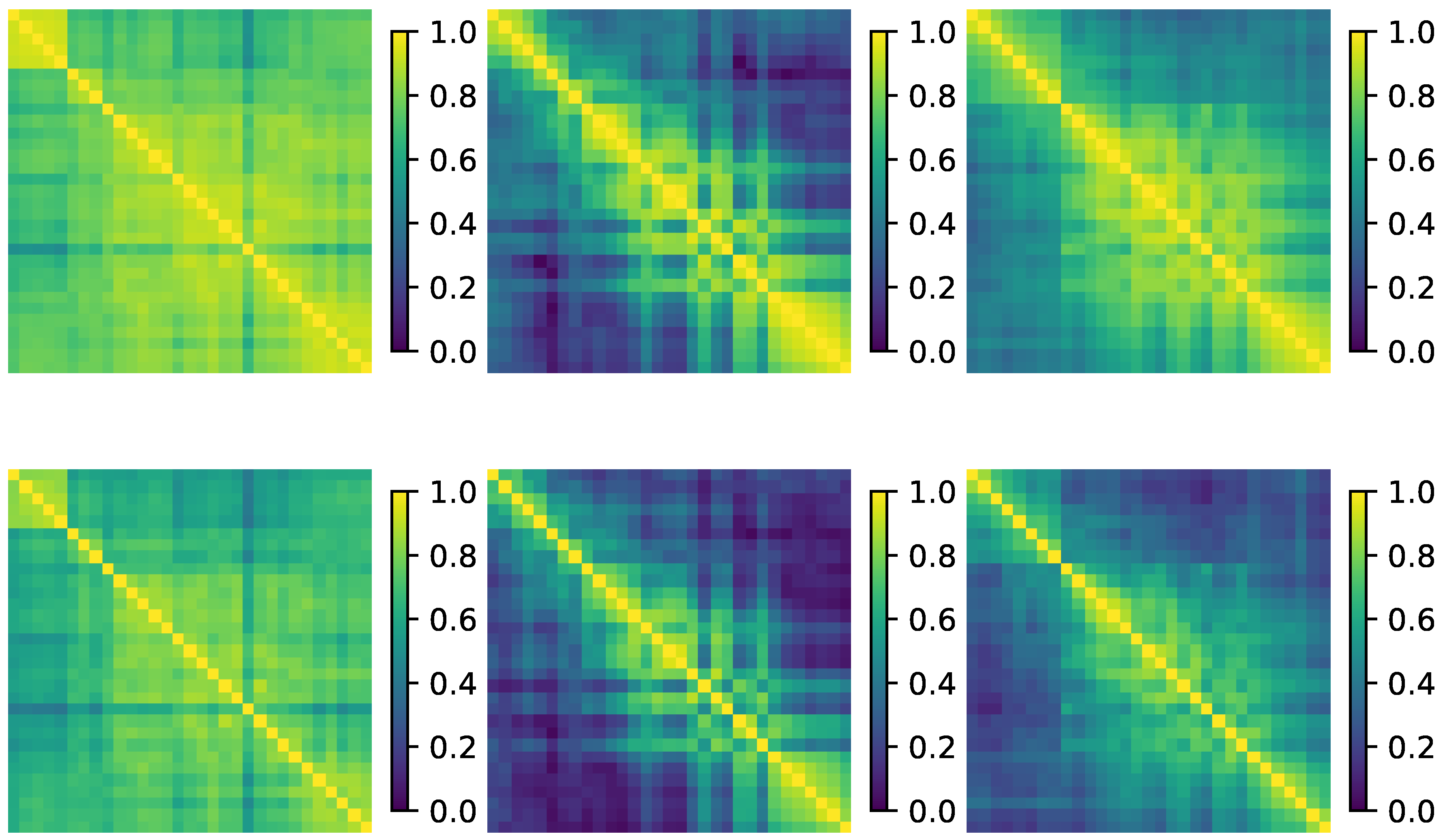
Figure 6.
A heat plot of SCM entries of synthetic data versus real data showing absolute value (left), and phase (right). The red line is the reference and the blue line is the mean of synthetic data, with blue error bars showing the standard deviation of the synthetic data.
Figure 6.
A heat plot of SCM entries of synthetic data versus real data showing absolute value (left), and phase (right). The red line is the reference and the blue line is the mean of synthetic data, with blue error bars showing the standard deviation of the synthetic data.

Figure 7.
Top, the kernel used when computing the SCM for use in generating the synthetic data. Bottom, the kernel used when computing the SCM for the deformation retrieval methods. Both kernels are Gaussian and have been normalized to have mass one.
Figure 7.
Top, the kernel used when computing the SCM for use in generating the synthetic data. Bottom, the kernel used when computing the SCM for the deformation retrieval methods. Both kernels are Gaussian and have been normalized to have mass one.
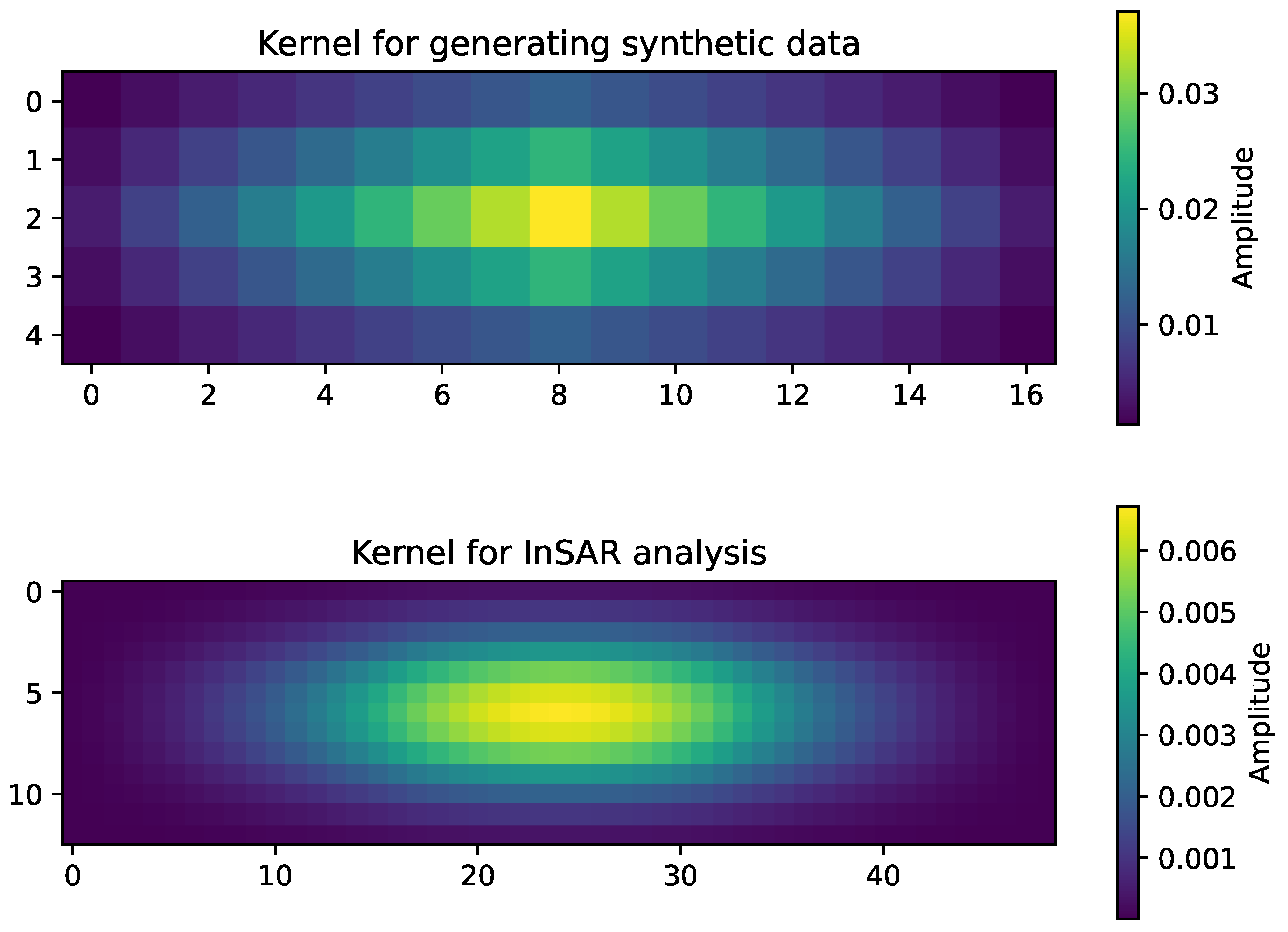
Figure 8.
Left shows the cumulative deformation derived from real data. Right shows the standard deviation of the recovered deformations derived from synthetic data. Top shows results for Method 1, while bottom shows results for Method 2.
Figure 8.
Left shows the cumulative deformation derived from real data. Right shows the standard deviation of the recovered deformations derived from synthetic data. Top shows results for Method 1, while bottom shows results for Method 2.
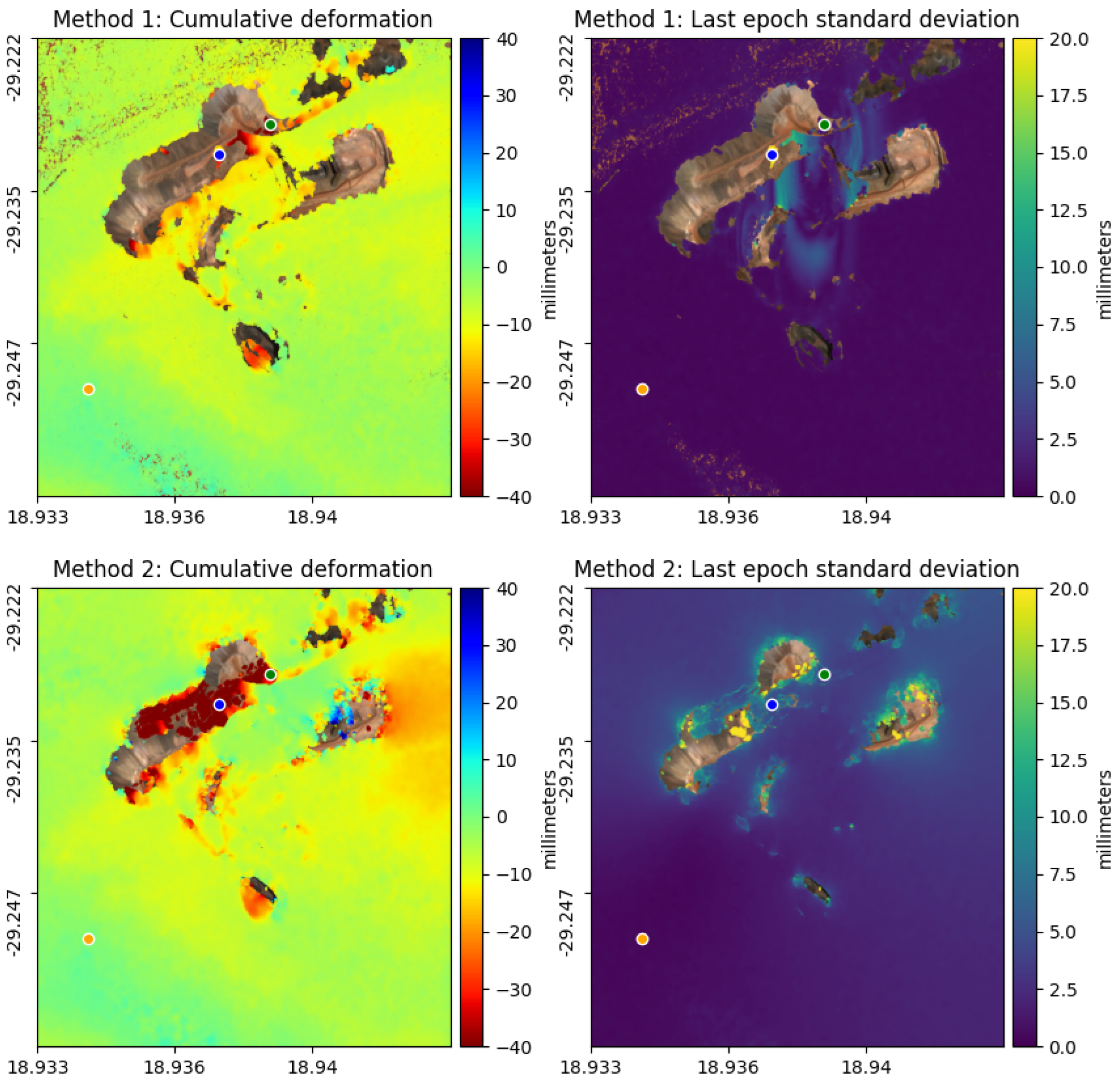
Figure 9.
Top shows the ensemble of deformation histories derived from synthetic data in green, and the deformation recovered from the real SAR data in red. Bottom shows the difference between the mean ensemble deformation and the deformation recovered from real data. The error bars are the standard deviation of the ensemble of deformation histories. Left shows Method 1, while right shows Method 2. This is for deformation at the green point relative to the orange point as shown in Figure 3.
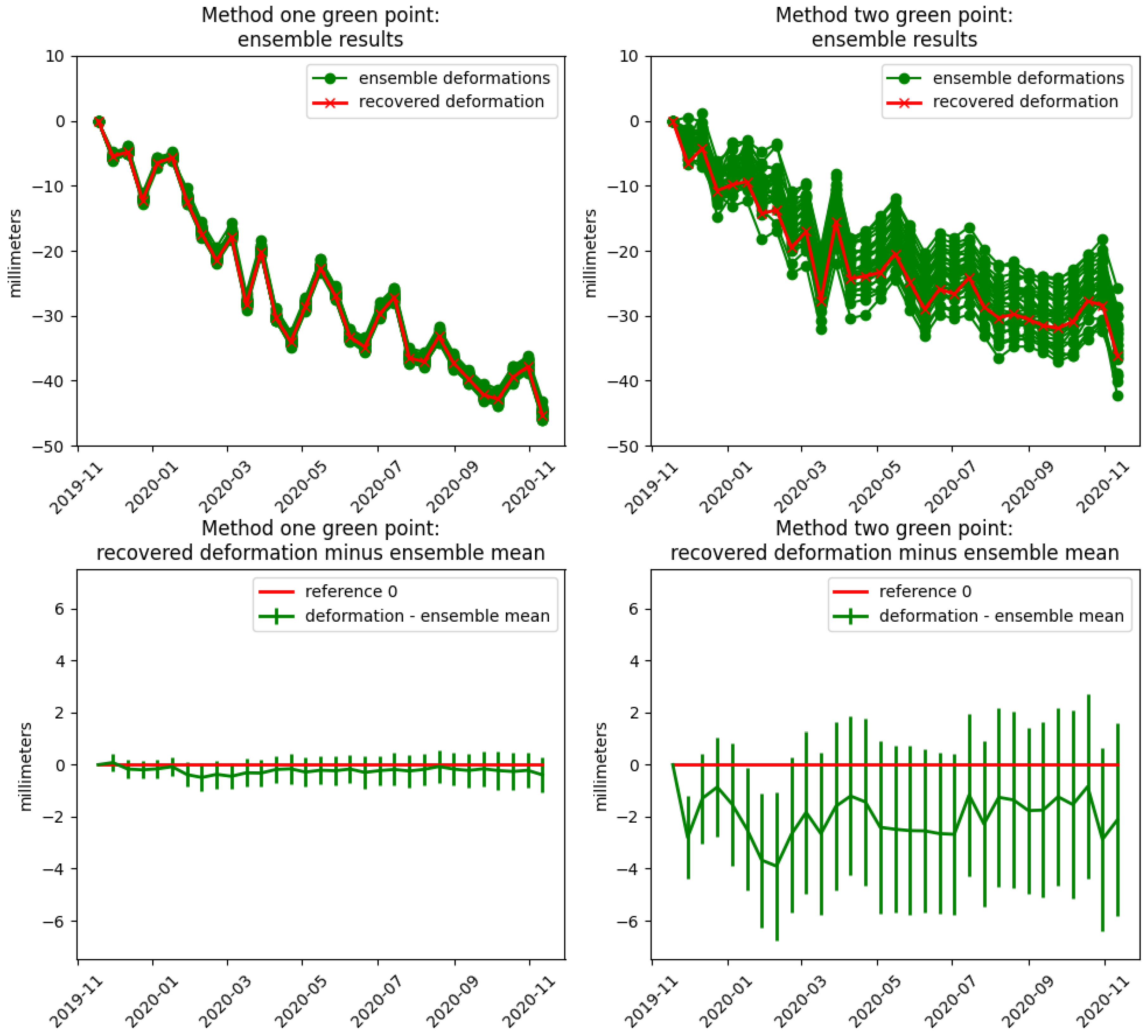
Figure 10.
Top shows the ensemble of deformation histories derived from synthetic data in blue, and the deformation recovered from the real SAR data in red. Bottom shows the difference between the mean ensemble deformation and the deformation recovered from real data. The error bars are the standard deviation of the ensemble of deformation histories. Left shows Method 1, while right shows Method 2. This is for deformation at the blue point relative to the orange point as shown in Figure 3.
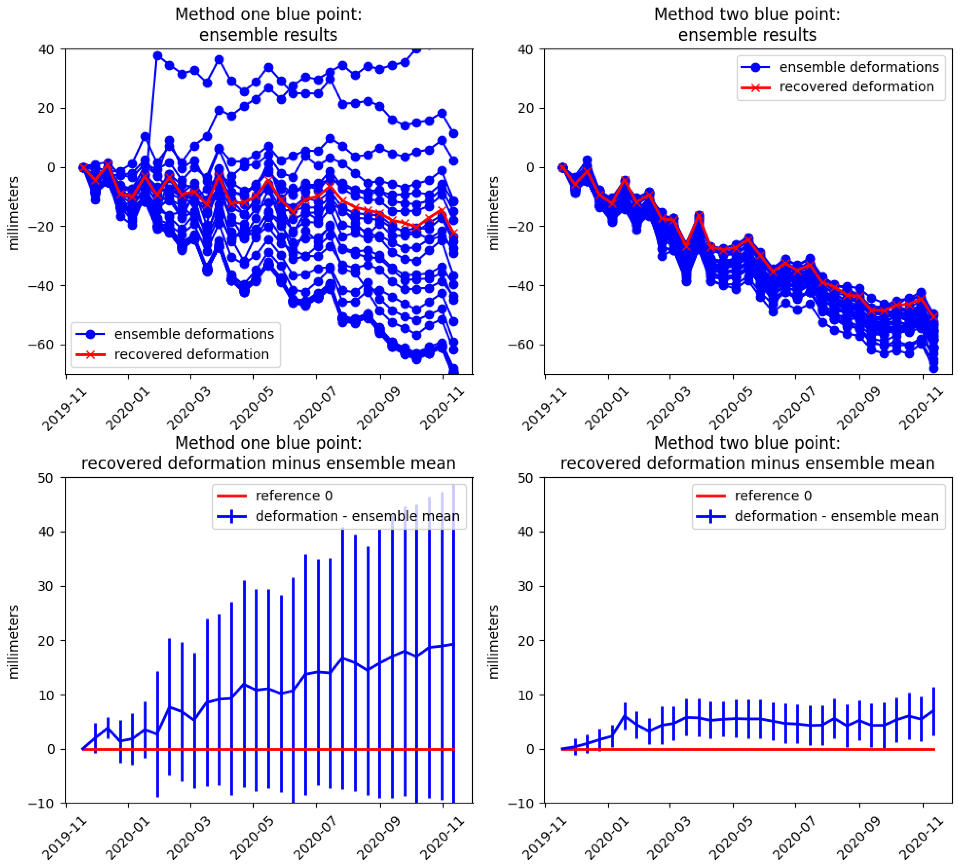
Figure 11.
A zoomed in view from the top right plot in Figure 8 focused around the blue and green points of the ensemble standard deviation of the cumulative deformation for Method 1.
Figure 11.
A zoomed in view from the top right plot in Figure 8 focused around the blue and green points of the ensemble standard deviation of the cumulative deformation for Method 1.
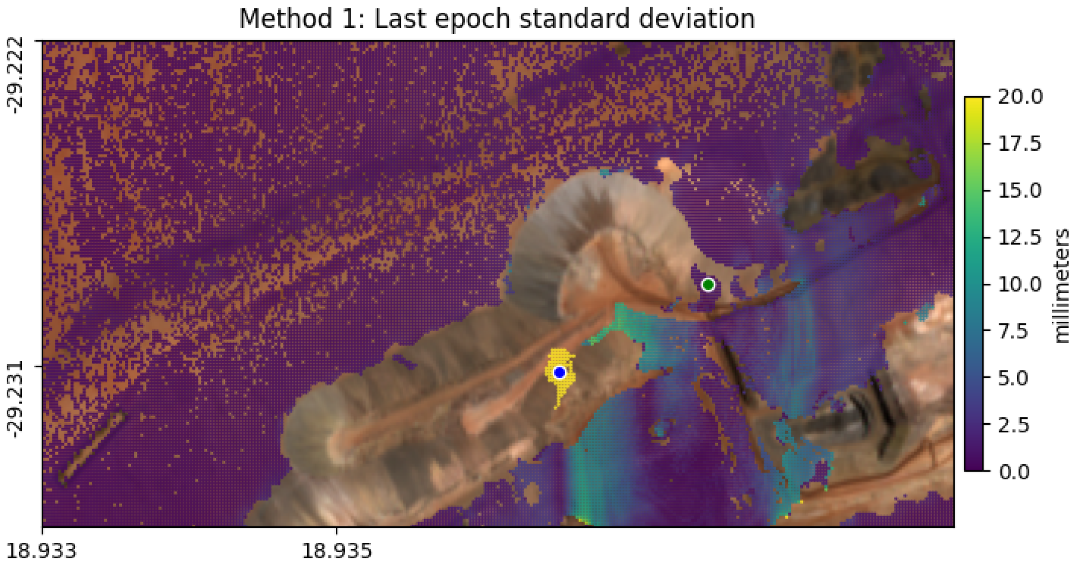

Table 1.
Summary of problem size and costs for the analysis of Method 1 and Method 2.
| Method 1 | Method 2 | |
|---|---|---|
| Number of epochs | 31 | 31 |
| Number of selected points | 137177 | 157546 |
| Number of ensemble instances | 30 | 30 |
| Co-registration (vCPU hours) | 0.86 | 0.86 |
| Matrix square root (vCPU hours) | 0.34 | 0.27 |
| All InSAR analyses (vCPU hours) | 117.07 | 200.95 |
| Dispatch (vCPU hours) | 5.51 | 4.6 |
| Storage for co-registered SAR scenes (GB) | 6.28 | 6.28 |
| Temporary storage of matrix square root (GB) | 4.78 | 4.78 |
| Storage for all InSAR results (GB) | 0.56 | 0.63 |
Disclaimer/Publisher’s Note: The statements, opinions and data contained in all publications are solely those of the individual author(s) and contributor(s) and not of MDPI and/or the editor(s). MDPI and/or the editor(s) disclaim responsibility for any injury to people or property resulting from any ideas, methods, instructions or products referred to in the content. |
© 2023 by the authors. Licensee MDPI, Basel, Switzerland. This article is an open access article distributed under the terms and conditions of the Creative Commons Attribution (CC BY) license (http://creativecommons.org/licenses/by/4.0/).
Copyright: This open access article is published under a Creative Commons CC BY 4.0 license, which permit the free download, distribution, and reuse, provided that the author and preprint are cited in any reuse.


