
Submitted:
31 March 2023
Posted:
03 April 2023
You are already at the latest version
Abstract
The deep energy method (DEM), a type of physics-informed neural network, is evolving as an alternative to finite element analysis. This method employs the principle of minimum potential energy to predict deformations under static loading conditions. However, the model’s accuracy is contingent upon choosing the appropriate architecture for the model, which can be challenging due to the high interactions between hyperparameters, large search space, difficulty in identifying objective functions, and non-convex relationships with the objective functions. To improve DEM’s accuracy, we first introduce random Fourier feature (RFF) mapping. RFF mapping helps with the training of the model by reducing bias towards high frequencies. The effects of six hyperparameters are then studied under compression, tension, and bending loads in planar linear elasticity. Based on this study, a systematic automated hyperparameter optimization approach is proposed. Due to the high interaction between hyperparameters and the non-convex nature of the optimization problem, Bayesian optimization algorithms are used. The models trained using optimized hyperparameters and having Fourier feature mapping can accurately predict deflections compared to finite element analysis. Additionally, the deflections obtained for tension and compression load cases are more sensitive to variations in hyperparameters than bending.
Keywords:
Elasticity
; Machine learning
; Minimum potential energy
; Partial differential equations (PDEs)
; Physics-informed neural network
1. Introduction
With the advancements in computational technology and complexity in design, engineers seek to predict the component’s performance before it can be manufactured. These predictions involve complex boundary value problems (BVP), which require solutions to partial differential equations (PDEs). Typically, these PDEs are solved through numerical approximations. In solid mechanics, conventional methods to solve PDEs include mesh-free methods1,2, finite element analysis (FEA)3, and isogeometric analysis4,5. However, these methods are poised with challenges, such as obtaining robust and accurate solutions for ill-posed, high-dimensional, or coupled problems, to name a few.
Machine learning methods are rapidly developing as an alternative to traditional approaches to minimize or, in some cases, eliminate the issues mentioned above. Liu et al.6 have discussed FEA’s evolution, future, and transition to machine learning applications in detail. In the case of solid and fluid mechanics, machine learning models can broadly be classified into data-driven models6,7,16,17,8–15 and physics-informed neural networks (PINNs)18–25. In data-driven models, data from experimental and computational results are used to train the models. Although data-driven models can capture complex physical phenomena, the amount of data required to train the models, data quality, and data generation process impede its widespread implementation26. Another application of data-driven models in mechanics is to provide an automated framework for predicting constitutive models for material behavior, as discussed by Flaschel et al.27, Yang et al.28, and Chen29. The data-driven models can also take images to identify the material distribution and defect characterization30. To reduce dependency on a large data set, Saha et al.31 developed a model (hierarchical deep learning neural network (HiDeNN)) with universal approximation capability to interpolate between data points for extremely nonlinear relationships.
In contrast to data-driven models, PINNs use a deep neural network (DNN) to train the model based on physical laws at a set of points in the domain. PINNs with automatic differentiation were first introduced by Raisi et al.18. They have several advantages over data-driven models as they do not require data labeling and require no or minimal preliminary datasets compared to purely data-driven models. Two types of PINN models are rapidly developing in solid mechanics: deep collocation method (DCM)23–25,32 and deep energy method (DEM)33–35. In DCM, residuals of strong form define the loss function at points sampled from the physical domain, corresponding boundary, and initial conditions (collocation points). This method has been extended and improved by researchers36,37. Haghighat et al.38 used a PINN technique to solve the coupled flow and mechanical deformation equations in porous media for single-phase and multiphase flows. Improving the application of PINNs to irregular geometries, Gao et al.39 developed PhyGeoNet, a convolutional neural network model (CNN) that could learn solutions for parametric PDEs on irregular domains using elliptic coordinate mapping. Chen et al.40 generalized the PINNs to discover governing PDEs from sparse and noisy data. Though the DCM has been widely successful in predicting outcomes, the approach requires higher-order gradients, which can be computationally expensive.
In the case of DEM, the system’s potential energy (PE), expressed as a loss function, is minimized to predict the system’s displacements. Compared to classical PINNs, DEM has advantages as it relies only on first-order differentiation to train the neural network and on accurate numerical integration. The DEM method can be extended to the problems where an energy function exists and reduces dependencies on PDEs of the base function. E and Yu41 first proposed the idea of DEM using the Ritz method to solve variational problems. Nguyen-Thanh et al.34 expanded the work presented by E and Yu to 2D and 3D material models. Implementation of DEM for several BVPs has been reported in the literature33,35,42. Extending this work, Fuhg and Bouklas43 demonstrated that DEM and DCM fail to accurately resolve displacement and stresses at stress concentration regions. They proposed modified DEM (mDEM) to overcome this issue and added stresses to the loss function. However, it is worth noting that including stresses in the loss function requires a second-order differential equation. The modification allowed the successful resolution of stresses around the stress concentration regions. Abueidda et al.44 enhanced the model by developing PINN that combines residuals of the strong form and the system’s potential energy. The proposed formulation yielded a loss function with multiple loss terms. As a result, the coefficient of variation weighting scheme was also introduced in the loss function to assign the weight dynamically and adaptively for each term. He et al. extended the applicability of DEM to plasticity45 and graph convolutional network46. Similar to DEM, Sun et al.47 used DNN to develop surrogate models for fluid flows using a loss function that incorporated initial boundary conditions and governing PDEs. One of the disadvantages of PINNs over classical FEA is the time required to train the neural network model. However, users can use transfer learning48,49, where instead of retraining the model from scratch, the network can either be partially retrained, trained using prior weights and biases, or use a trained model to predict mechanics for similar geometry.
Though DEM has been successfully used to predict deformations in bending, similar accuracies were not obtained for compression and tension loadings, even for a simple 2D rectangular linear elastic plate. Figure 1 shows the deformation under compression loading in the y-direction using the architecture proposed by Nguyen-Thanh et al.34. The geometry and boundary conditions for the plate are shown in Figure 7. From Figure 1, we can notice that even though symmetric pressure is applied on the plate, the resulting displacements obtained from DEM are not symmetric. Thus, there is a need to improve the accuracy of DEM under generalized loading conditions.
In this paper, two modifications are proposed to improve the accuracy of DEM while retaining dependency only on first-order derivatives. Firstly, random Fourier feature mapping is introduced in the multilayer perceptron (MLP) model to reduce bias that may be present during the model’s training. Secondly, a two-loop architecture is proposed to obtain appropriate hyperparameters for a given geometry. Recent studies have demonstrated that optimizing hyperparameters in large and multi-layered models impedes scientific progress50. This process can be challenging for DEM due to the high interaction between independent hyperparameters, large search space, difficulty in identifying objective functions, and non-convex relationships with the objective functions. Thus, the effect of different hyperparameters in loss function and the effect of loss function on displacement are also studied to find a generalized search space.
Tuning these hyperparameters through manual trial and error is highly time-consuming. As a result, researchers have employed grid search, random search, and optimization algorithms to obtain the best combination of hyperparameters22,50–53. Still, studies on optimizing hyperparameters and architectures of PINNs for solving mechanics problems remain uncommon. Wang et al.54 proposed Auto-PINN, a framework for employing Neural Architecture Search (NAS) techniques for PINNs to solve heat transfer problem. However, unlike Wang et al.54, we found that not all hyperparameters can be decoupled for DEM.
In addition, the L2 norm is commonly employed as an objective function to obtain optimized hyperparameters. This approach requires finding a solution to the BVP beforehand. Since hyperparameters can be problem-specific, using the L2 norm as an objective function increases the dependency of PINNs on existing solutions, reducing their generalizability. The current research demonstrates that the principle of minimum potential energy can be used as an alternative objective function to obtain optimized hyperparameters. This approach mitigates the need for prior knowledge of the solution. The examples presented in the current research are based on 2D linear elastic plane stress problems. Even though the examples solved in this study involve 2D linear elastic material models, the proposed approach can be extended to a variety of DEM problems (for example, to 3D and nonlinear material models). Random Fourier feature (RFF) mapping (discussed in Section 3) is introduced to improve the accuracy of DEM further. RFF mapping helps in reducing bias during learning towards high frequencies. The effect of reduction in bias becomes prominent in complex geometries and loading conditions.
The paper is divided into eight sections. Section 2 and Section 3 describe the formulation of DEM and modifications made to DEM (m-DEM). Preliminary observations relating the accuracy of displacements obtained from DEM to the loss function and hyperparameters are discussed in Section 4. Based on initial observations, a search space is defined and followed by hyperparameter optimization for the elastic rectangular plate in Section 5. The transferability of optimized hyperparameters obtained in Section 5 to different geometry and load cases is discussed in Section 6. The effect of adding RFF mapping in MLP is shown in Section 7. Finally, conclusions are presented in Section 8.
2. DEM formulation
The DEM consists of a multilayer perceptron (MLP) neural network, as shown in Figure 2. In general, MLP consists of sets of neurons arranged in layers. Each neuron is connected to all the neurons in adjacent layers. The number of layers (N) and neurons in each layer are predefined according to specific applications. In DEM, the number of neurons in the first and last layer (also known as input and output layers, respectively) is determined by the system’s dimension (two in the case of 2D and three in 3D). The programmer predefines the number of neurons in the layers between the input and output layers (also called hidden layers).
Mathematically, the value of each neuron connecting the previous layer ( is calculated using a linear combination of weights (w) and biases (b), as shown in Equation 1. An activation function (φ: ℝ→ ℝ) then operates on the calculated value to determine the value passed by the neuron.
The values of weights and biases are determined such that the loss function ( or ) is minimized. In a so-called backpropagation procedure, an optimization algorithm can be used to iterate over the loss function to predict values of weights and biases such that:
Limited-memory Broyden–Fletcher–Goldfarb–Shanno (L-BFGS) algorithm is used in the examples shown in the following sections to minimize the loss function and demonstrate the performance of DEM. However, other algorithms can also be used. The backpropagation capabilities of PyTorch are used to calculate gradients of the loss function.
In the above description, parameters like the number of layers and of neurons in each layer need to be defined before MLP can be trained. These parameters, called hyperparameters, define the architecture of the MLP and control the learning process of the model. It is essential to obtain optimized values for the hyperparameters to achieve a minimum value for the loss function. The number of hyperparameters and their values vary according to the problem statement. Six hyperparameters based on the architecture of DEM were determined. These are the total number of layers, number of neurons in hidden layers, activation function, standard deviation for predicting weights and biases, learning rate for the L-BFGS algorithm, and the number of epochs for the L-BFGS algorithm.
The loss function for DEM is defined as the system’s potential energy (Equation 3), where U is the system’s internal energy, W is the energy due to externally applied load, is a kinematically admissible displacement field, H is the space of admissible functions, is strain energy density function, are internal forces of the body B, and are traction forces applied to the area (Figure 3).
The selection of loss function is based on the principle of minimum potential energy: out of all the possible kinematically admissible deformations, a conservative structural system assumes displacements that minimize total potential energy at equilibrium.
3. Modifications to DEM
3.1. Random Fourier feature mapping
Fourier transformation converts functions dependent on space or time domain into functions dependent on spatial or temporal frequency. This transformation is widely used in mathematics and digital image processing to simplify calculations. Tancik et al.55 demonstrated that the standard MLP fails to learn high frequencies, and Fourier feature mapping can be used to mitigate this bias. Wang et al.56 expanded the work of Tancik et al.55 to PINNs, discussed the limitations of PINNs via the neural tangent kernel theory (NTK), and illustrated how PINNs are biased towards learning along the dominant eigenvectors of their limiting NTK. Correspondingly, they have demonstrated that using Fourier feature mappings with PINNs helps modulate the frequency of the NTK eigenvectors.
Figure 4 shows the implementation of the Fourier feature mapping. The input layer (coordinates of the training points from the physical domain) is passed through a Fourier mapping γ before passing through MLP. The function γ maps the input coordinates to a higher-dimensional hypersphere using a set of sinusoids:
where hi’s are the Fourier basis frequencies used for approximation and ai represent the corresponding coefficients in the Fourier series. Here, we adopted Gaussian random Fourier feature (RFF) mapping. Each entry in h is sampled from a normal distribution N (0, σ2), where σ2 is the variance. σ is a hyperparameter that needs to be specified for each problem. Adding RFF mapping helped improve the solution’s accuracy even with optimized hyperparameters. The details on the effect of RFF mapping are discussed in Section 7.
3.2. Tuning of hyperparameters
Like most MLPs, the accuracy of DEM solutions depends on selecting appropriate hyperparameters. We will see in Section 4 that the hyperparameters are highly interdependent, and the search space is highly non-convex. In addition, even for a simplified linear elastic material model, getting stuck in local minima during hyperparameter tuning and obtaining incorrect solutions is relatively easy. A two-loop architecture (as shown in Figure 5) is proposed to overcome these issues and simplify the hyperparameter tuning. The two loops are referred to as the inner loop (solves DEM with Fourier feature mapping) and the outer loop (used for hyperparameter tuning).
Three essential things must be considered to initialize a successful hyperparameter optimization: search space, optimization algorithm, and objective function. The selection of search space is discussed in detail in Section 4. Since the search space is non-convex and consists of continuous and discrete variables, a Bayesian optimization algorithm in the HyperOpt library (tree pazen estimator: TPE) was selected for the current study57. It is worth noting that the algorithms used for optimizing hyperparameters are an evolving field, and new algorithms are being rapidly developed. However, the selection of the best optimization algorithm for DEM is outside the scope of the current study.
Minimization of PE (Equation 3) was chosen as the objective function for hyperparameter tuning. The selection was based on the principle of minimum potential energy. The advantages of choosing minimal PE are minimized additional calculations required during the tuning process and no required prior knowledge of the solution. Thus, the framework can be extended to any problem statement that can be solved using DEM, and hyperparameters can be turned to specific BVP if required without knowledge of the exact solution. The algorithm for the tuning process is described in Figure 6. A BVP is defined along with search space and profiles for hyperparameters. The hyperparameters are initialized randomly based on the search space and supplied to DEM. DEM then solves for weights and biases to obtain displacements for minimum PE. Once convergence has been reached, the value for minimum PE is supplied to the outer loop, where an observation set D is formed. A surrogate model is formed using D to predict the next set of hyperparameters. The new hyperparameters are supplied to the inner loop, which runs DEM to solve for BVP and supplies minimum PE. D is updated based on new results. The cycle continues until the termination condition is satisfied. We used two termination conditions for examples discussed in Section 5. The first condition asks the algorithm to be terminated if no improvement in minimum PE is observed for thirty consecutive iterations. This condition also specifies the minimum number of iterations that need to be undertaken by the algorithm. The second condition asks for the algorithm to be terminated after fifty iterations. The condition can be varied according to the maximum number of iterations that should be run for hyperparameter tuning.
The initial TPE algorithm was proposed by Bergstra et al.58. This approach employs both estimator models p(x|y) and p(y) to reduce computations. It transforms the prior distribution of the search space into truncated Gaussian distribution and modifies the posterior distribution based on observations. It then sorts the target value (y) and divides it into two, as shown in Equation 5.
where is the boundary used to segregate the target value, is the density formed by observations that are less than , and g(x) is the density formed by the remaining observations. The TPE algorithm chooses to be some quantile ζ of the observed y values so that p(y < y∗ ) = ζ. The next promising point is chosen based on the Expected Improvement (EI) criterion59.
4. Pre-experiments and observations
The dependency of PE on hyperparameters can be best understood using a simplified BVP. Thus, an elastic plate subjected to compression and bending loads (shown in Figure 7) is shown as an example. The plate is 4 mm in length and 1 mm wide. It is composed of an elastic material having young’s modulus of 1000 MPa and Poisson’s ratio of 0.3. The plate is subjected to uniform compression and bending loads, as shown in Figure 7b,c. For compressive load, a uniform compressive pressure of 50 MPa was applied to the right, while the left end was fixed in all degrees of freedom. In the case of bending loads, a uniform transverse shear load of 10 MPa, forcing the plate to move downwards, was applied on the right, and the left end was fixed in all degrees of freedom. The strain energy density of the plate is given by:
where and are Lame constants. is the strain tensor for small deformations, which is related to displacements by:
The relationships between the Lame constants, young’s modulus (E) and Poisson’s ratio (ν) are given by equation 9.
Differentiation of strain energy density with respect to strain tensor provides Cauchy stress tensor , which can be differentiated again to find the stiffness tensor C.
For a 2D plane stress condition the relation between Cauchy stress tensor and strain tensor can be reduced to:
4.1. Interactions effect
Sensitivity analysis can be used to determine the impact of independent inputs (hyperparameters) on outputs (PE under compression and bending). A five-level Taguchi design of experiment (DOE) and two-level half-factorial DOE were employed to obtain the dataset for sensitivity analysis. The values of hyperparameters used to generate a five-level Taguchi DOE are shown in Table 1. Levels 1 and 5 from Table 2 were utilized to design the two-level half-factorial DOE.
After running m-DEM, the minimum potential energy corresponding to each set of hyperparameters was collected, and the data were analyzed using Minitab. Similar results were obtained for compression and bending loads. The results obtained from compression loading conditions are discussed in this section.
The analysis of the data was conducted using Minitab. Figure 8 and Figure 9 show the main effect and interaction plots between hyperparameters. Figure 8 illustrates that the mean response (minimum PE) varies for each hyperparameter. We also notice that the minimum PE obtained from DEM does not follow the same trends across hyperparameters, and it varies least with the variation in activation function.

Table 2.
Values used to generate data for sensitivity analysis.
| Variable | Level 1 | Level 2 | Level 3 | Level 4 | Level 5 |
|---|---|---|---|---|---|
| Learning Rate | 0.1 | 0.368 | 1 | 2.718 | 7.389 |
| Neurons | 20 | 52 | 70 | 96 | 120 |
| Standard Dev (DNN) | 0.0001 | 0.001 | 0.01 | 0.1 | 1 |
| Standard Dev (RFF) | 0.0001 | 0.001 | 0.01 | 0.1 | 1 |
| Total number of layers | 3 | 4 | 5 | 6 | 7 |
| Activation function | rrelu | relu | celu | sigmoid | tanh |
Figure 9 helps us visualize significant interaction effects between the hyperparameters even though each can be varied independently. Due to the high interaction, multiple hyperparameters should be varied simultaneously for tuning the hyperparameters. This process can be very tedious and time-consuming if done manually. Alternatively, computational algorithms can be used to speed up the process.
In addition to plotting the main effects plot and interaction plot, the normality of the loss function obtained from two DOE was tested using the Anderson-Darling test. Figure 10 shows the probability plot for the loss function. Based on the test results, we can notice that the data is not normally distributed (p-value <0.005). We can also see the high probability of obtaining a loss function near -4.5. The importance of this observation is discussed later in this section.
Loss functions from five hundred DEM iterations were collected to further study the six hyperparameters’ effect. The hyperparameters were varied using the random algorithm present in HyperOpt. The minimum potential energy obtained from the iterations plotted against hyperparameters is shown in Figure 11. However, from this figure, we do not see any trend between hyperparameters and the loss function.
4.2. Sensitivity of loss functions and displacements
Figure 11 shows that the loss function for most iterations lies in a narrow range of -5 to -4.5. Displacements in the y-direction for two randomly picked iterations are shown in Figure 12. From this figure, we can see that even though the variation in loss function is relatively small, neither provides the correct displacement prediction. Previously we had observed that the loss function is not normally distributed, and without a trend, it is not easy to tune hyperparameters manually. This observation further strengthens the requirement for a systematic approach to tuning hyperparameters.
5. Tuning hyperparameters for different load cases
In the previous section, we concluded that all six hyperparameters are interdependent. However, from the main effects plot (Figure 8), we can estimate that the activation function has a lesser impact on the loss function than other parameters. From random five hundred iterations, we see that the median loss function for rrelu and sigmoid is less than other employed activation functions. As a result, the activation function could be fixed to one of them, and here we select rrelu. Further, the number of layers was fixed to five. The other four hyperparameters varied according to the sensitivity profiles and ranges provided in Table 3.
Table 3.
Parameter ranges and profiles.
| Hyperparameter | Sensitivity profile | Range |
|---|---|---|
| Learning Rate | loguniform | Exp(0-2) |
| Neurons | quniform | 20-120 |
| Standard Dev (DNN) | uniform | 0-1 |
| Standard Dev (RFF) | uniform | 0-1 |
Sensitivity profile and ranges together define the search domain. While the range provides the upper and lower bounds for each hyperparameter, the sensitivity profile influences how values are selected within the range. A profile of loguniform returns values drawn from the natural log, such that the natural log of the returned value is uniformly distributed. Quniform returns discrete values between the upper and lower bounds, and uniform profile returns a value uniformly between the upper and lower bounds.
The framework described in Section 3 was used to tune hyperparameters for the two load cases specified in Figure 7. The Python code developed for the framework was run on Delta supercomputer at the National Center for Supercomputing and Applications at the University of Illinois at Urbana-Champaign using an A100 single-node GPU consisting of a single AMD 64-core processor with 256 GB DDR4-3200 RAM. The optimized hyperparameters for the two load cases obtained using Tree-structured Parzen Estimator (TPE) optimization algorithms are shown in Table 4. All the cases were analyzed using 100x50 training points over the computational domain, as shown in Figure 13. Simultaneously, FEA was also undertaken using Abaqus using element type CPS4R. The results obtained from FEA were assumed to be ground truth. The deviation of displacement predicted by DEM (using tuned hyperparameters) from those obtained from FEA was calculated using the L2-norm given by Equation 10.
Table 5.
Optimized hyperparameters for compressive and bending loads.
| Hyperparameter | Compression | Bending |
|---|---|---|
| Learning Rate | 1.35145 | 1.40475 |
| Neurons | 106 | 98 |
| Standard Dev (DNN) | 0.01977 | 0.03276 |
| Standard Dev (RFF) | 0.46094 | 0.49815 |
| Loss function | -4.98435 | -13.34657 |
| L2-error | 0.000019 | 0.000037 |
| Optimization time | 8 min 13 sec | 12 min 12 sec |
6. Transferability of hyperparameters
Though hyperparameters can be optimized for different load cases and plate geometry, multiple DEM iterations must be undertaken, which can be time-consuming. Thus, we explored the transferability of hyperparameters to different geometries and load cases to minimize this issue. The optimized hyperparameters found during compressive loading (mentioned in Table 5) are used for the following examples.
6.1. Transferability of hyperparameters to different load cases
The optimized hyperparameters obtained for compression load case were used to predict displacements under tensile and bending loads. For the tensile test, a tensile pressure of 50 MPa was applied on the right end of the plate. Figure 14 shows predicted displacements for all three load cases. To obtain the displacements under tensile loading, 32.975 seconds were taken to train the DEM model and 0.0067 seconds to evaluate the model (to obtain displacements). Even though the parameters were optimized for compression, we notice that it can also predict deformation under uniform tensile and bending loading with L2 errors of 1.95e-05 and 0.00192, respectively. Figure 15 shows deviations in predicted displacements for all three load cases compared to FEA.
6.2. Transferability of hyperparameters to different numerical resolution
The plate was discretized in 200 x 50 and 100 x 100 points instead of 100 x 25 points. The discretization was varied to understand the transferability of hyperparameters with variation in numerical resolution. Figure 16 shows the displacements obtained for the compressive load case in the y-direction. The figure shows that for selected hyperparameters, the displacements are not resolution dependent. To obtain the displacements for 200 x 50 and 100 x 100 points, 32.7134 seconds and 32.7906 seconds were taken to train the DEM model, and 0.0065 seconds and 0.0065 seconds were taken to evaluate the models, respectively. We notice that the resolution does not significantly affect the computational time.
6.3. Transferability of hyperparameters across geometry
A 1 mm x 1 mm plate was subjected to uniaxial compression using 25 x 25 points, as shown in Figure 17a. The training points used for DEM are shown in Figure 17b. From Figure 18, we can conclude that in DEM, the optimized hyperparameters can be used to predict displacements for geometries different from which they were optimized. 11.553 seconds were taken to train the model, while 0.0055 seconds were taken to evaluate the model. We notice that the time taken to train the model decreases as the geometry size decreases. This observation can be used in the future to reduce the time required to obtain optimal hyperparameters.
In addition, we also analyzed the transferability of DEM (with RFF mapping) to predict displacements for geometries for which it was not trained. In the following example, the DEM model was trained using a 4 mm x 1 mm plate subjected to a compressive load of -10 MPa. The trained model was then used to predict displacements produced in a 1 mm x 1 mm plate. 32.229 seconds were taken to train the model while, 0.0041 seconds were taken to evaluate the model. The results are shown in Figure 19. Even though the DEM model was trained for a plate of dimensions 4 mm x 1 mm, it can still predict displacements in the plate sized 1 mm x 1 mm subjected to similar boundary conditions.
6.4. Transferability of hyperparameters to partial loading
In this example, a load is applied locally on the upper right-hand corner of a 4 x 1 mm2 plate (Figure 20). The same number of domain and boundary training points is used in Section 4. The displacement obtained from DEM, FEA, and error in prediction compared to FEA are shown in Figure 21. To obtain displacement under partial loading DEM model was trained in 43.332 seconds. 0.066 seconds were taken to obtain displacements for the model under evaluation.
Figure 21 shows that DEM can predict displacement under localized traction using the optimal hyperparameters parameters obtained from uniform compression. However, the magnitude of error increases by order of magnitude. We also notice again that the error in displacements is proportional to the magnitude of displacement in each direction.
6.5. Transferability of hyperparameters to a random geometry
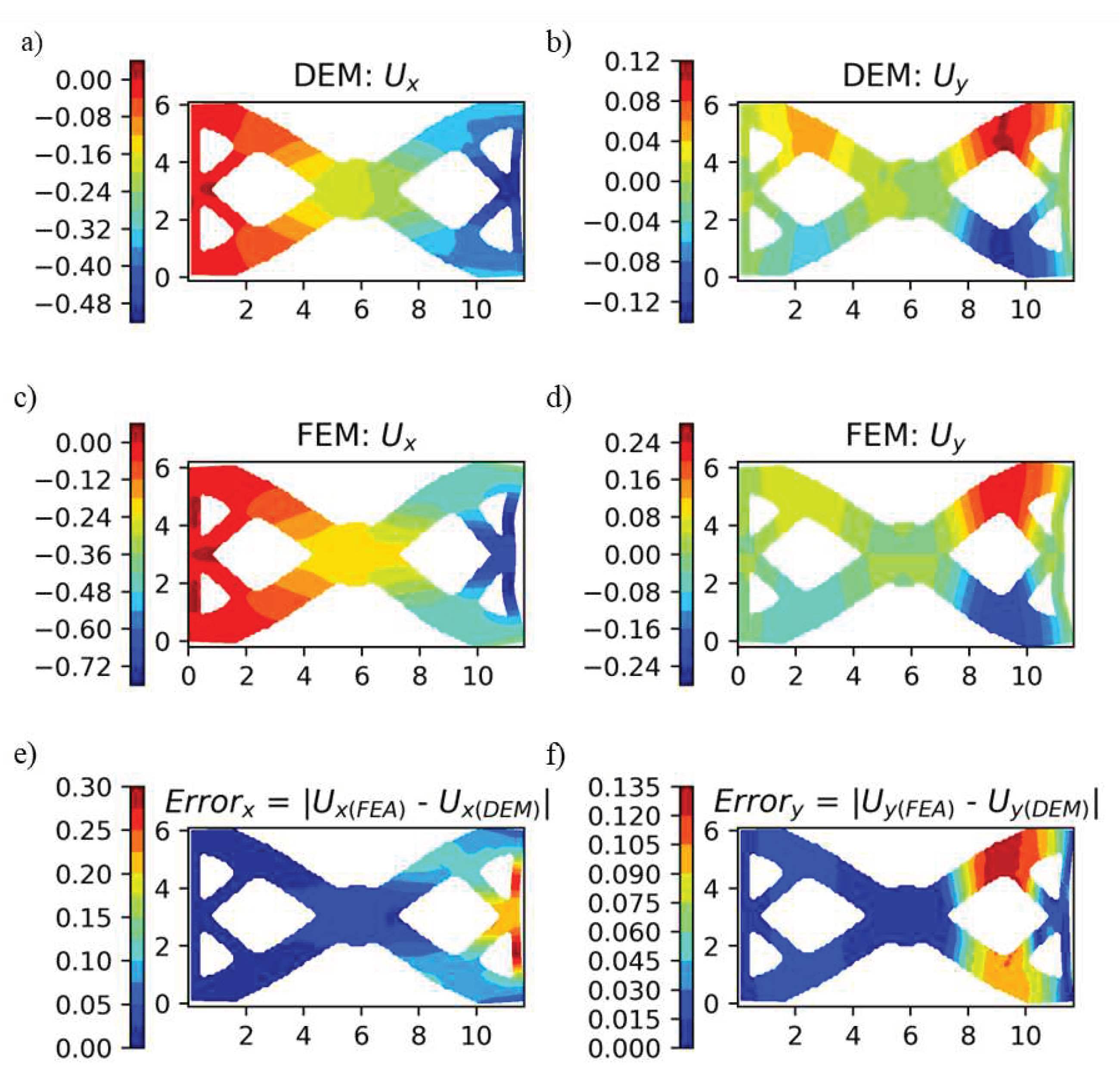
In the previous section, only simplified geometries were studied. To analyze the transferability to complex geometries, passive elements were introduced by multiplying the corresponding strain energy of the element with their material density. Since passive elements do not contribute to internal energy, the material density corresponding to passive elements was zero. A random geometry of density distribution, shown in Figure 22, was introduced. A uniform compressive load of 10 MPa was applied at the right end of geometry, while the left end was fixed in all DOF. The displacements obtained from the DEM model are shown in Figure 23. The figure shows that even though the hyperparameters were optimized for a simplified rectangular plate, they can be used to predict displacements in complex geometry.
7. Effect of introducing RFF mapping
In earlier examples, RFF mapping was introduced in MLP to reduce the bias in the model’s training (as discussed in Section 3). In this section, the models are trained without RFF mapping to study its effect. As discussed in previous sections, hyperparameters are interdependent. Thus, hyperparameter tuning was undertaken for a 4x1mm2 plate subjected to compressive loads. The procedure discussed in the above sections was followed. The optimized hyperparameters are shown in Table 6.
Table 6.
Optimized hyperparameters for compressive load.
| Hyperparameter | Compression |
|---|---|
| Learning Rate | 1.00118 |
| Neurons | 98 |
| Standard Dev (DNN) | 0.05492 |
The displacements obtained from DEM without RFF mapping for three different cases: uniform compression of 4x1 mm2 plate, uniform bending of 4x1 mm2 plate, and uniform compression of a random geometry are shown in Figure 24, Figure 25 and Figure 26. Comparing the error in displacements under compression loading (Figure 24e, 24f) with the error when RFF mapping was present (Figure 15a, 15b), we can conclude that no significant difference exists between the two cases. However, while comparing the errors under bending and random geometry (Figure 15e, 15f with Figure 25e, 25f, and Figure 23e, 23f with Figure 26e, 26f), we conclude that displacements predicted with RFF mapping are more accurate than the displacements predicted without RFF mapping. While comparing Figure 23e, 23f with Figure 26e, 26f, we notice that the error in displacements reduces by order of magnitude. Thus, the introduction of RFF mapping improved the accuracy of DEM and enabled the transferability of hyperparameters to wider geometries and boundary conditions.
8. Conclusions
This paper proposes a two-loop architecture to obtain DEM’s best architecture and hyperparameters. The inner loop predicts displacements and potential energy using DEM based on hyperparameters chosen by an outer loop. The outer loop receives the system’s potential energy from the inner loop, which depends on the architecture of ANN defined by hyperparameters. The optimization algorithm in the outer loop then searches the non-convex optimization space to identify hyperparameters for which minimum potential energy can be achieved. Fourier feature mapping is employed in the inner loop (DEM) to improve accuracy and simplify calculations. Six hyperparameters were chosen for the study. We found that the values of hyperparameters identified using this approach and the implementation of Fourier feature mapping produce displacements similar to those obtained through FEA (with an order of accuracy of O(h-3)).
Additionally, based on the examples presented in the paper, we conclude the following:
- The displacements obtained for tension and compression load cases are more sensitive to hyperparameters than displacements obtained for bending loads.
- With optimal hyperparameters, the order of accuracy for tension and compression load cases is lower than for bending loads.
- The optimal hyperparameters chosen through compression and tension load cases can predict displacement for different loading conditions and geometries. As a result, the optimal hyperparameters can be searched for a single loading condition and simplified geometry (depending on the desired accuracy).
- The error in predicted displacements is proportional to the magnitude of displacement.
- Generally, the activation function can be fixed to Randomized Leaky Rectified Linear Unit (rrelu) and the number of layers to 5. The two-loop architecture can then tune the hyperparameters for the given BVP.
- The accuracy of DEM and transferability of hyperparameters can be improved with RFF mapping.
Acknowledgments
The authors would like to thank the National Center for Supercomputing Applications (NCSA) at the University of Illinois at Urbana-Champaign, particularly its Industry Program, Research Consulting Directorate, and the Center for Artificial Intelligence Innovation (CAII) for their support and hardware resources. This research is also a part of the Delta research computing project, supported by the National Science Foundation (award OCI 2005572) and the State of Illinois.
Data Availability
The data supporting this study’s findings are available from the corresponding author upon reasonable request.
Code availability
The code for replication of our experiments will be available upon acceptance.
References
- Belytschko T, Rabczuk T, Huerta A, Fernández-Méndez S. Meshfree methods. In: Encyclopedia of Computational Mechanics. John Wiley & Sons, Ltd; 2004. [CrossRef]
- Belytschko T, Krysl P, Krongauz Y. A three-dimensional explicit element-free galerkin method. Int J Numer Methods Fluids. 1997;24(12):1253-1270. [CrossRef]
- Hughes TJR. The finite element method: linear static and dynamic finite element analysis. Dover Publications; 2012.
- Hughes TJR, Sangalli G, Tani M. Isogeometric analysis: mathematical and implementational aspects, with applications. Splines and PDEs: From Approximation Theory to Numerical Linear Algebra: Cetraro, Italy 2017 : ; 2018:237-315. [CrossRef]
- Hughes TJR, Cottrell JA, Bazilevs Y. Isogeometric analysis: CAD, finite elements, NURBS, exact geometry and mesh refinement. Comput Methods Appl Mech Eng. 2005;194(39-41):4135-4195. [CrossRef]
- Kim Y, Kim Y, Yang C, Park K, Gu GX, Ryu S. Deep learning framework for material design space exploration using active transfer learning and data augmentation. npj Comput Mater. 2021;7(1):140. [CrossRef]
- Rong Q, Wei H, Huang X, Bao H. Predicting the effective thermal conductivity of composites from cross sections images using deep learning methods. Compos Sci Technol. 2019;184:107861. [CrossRef]
- Koric S, Abueidda DW. Deep learning sequence methods in multiphysics modeling of steel solidification. Metals (Basel). 2021;11(3):494. [CrossRef]
- Fatehi E, Yazdani Sarvestani H, Ashrafi B, Akbarzadeh AH. Accelerated design of architectured ceramics with tunable thermal resistance via a hybrid machine learning and finite element approach. Mater Des. 2021;210:110056. [CrossRef]
- Spear AD, Kalidindi SR, Meredig B, Kontsos A, le Graverend J-B. Data-driven materials investigations: the next frontier in understanding and predicting fatigue behavior. JOM. 2018;70(7):1143-1146. [CrossRef]
- Gu GX, Chen C-T, Richmond DJ, Buehler MJ. Bioinspired hierarchical composite design using machine learning: simulation, additive manufacturing, and experiment. Mater Horizons. 2018;5(5):939-945. [CrossRef]
- Linka K, Hillgärtner M, Abdolazizi KP, Aydin RC, Itskov M, Cyron CJ. Constitutive artificial neural networks: A fast and general approach to predictive data-driven constitutive modeling by deep learning. J Comput Phys. 2021;429:110010. [CrossRef]
- Abueidda DW, Koric S, Sobh NA, Sehitoglu H. Deep learning for plasticity and thermo-viscoplasticity. Int J Plast. 2021;136:102852. [CrossRef]
- Qiu H, Yang H, Elkhodary K l., Tang S, Guo X, Huang J. A data-driven approach for modeling tension–compression asymmetric material behavior: numerical simulation and experiment. Comput Mech. 2022;69(1):299-313. [CrossRef]
- Liu WK, Karniadakis G, Tang S, Yvonnet J. A computational mechanics special issue on: data-driven modeling and simulation—theory, methods, and applications. Comput Mech. 2019;64(2):275-277. [CrossRef]
- Saurabh S, Sureka B. An evaluation of an unhealthy part identification using a 0d-1d diesel engine simulation based digital twin. SAE International Journal of Advances and Current Practices in Mobility 4 : ; 2022. [CrossRef]
- Mozaffar M, Bostanabad R, Chen W, Ehmann K, Cao J, Bessa MA. Deep learning predicts path-dependent plasticity. Proc Natl Acad Sci. 2019;116(52):26414-26420. [CrossRef]
- Raissi M, Perdikaris P, Karniadakis GE. Physics-informed neural networks: A deep learning framework for solving forward and inverse problems involving nonlinear partial differential equations. J Comput Phys. 2019;378:686-707. [CrossRef]
- Abueidda DW, Lu Q, Koric S. Meshless physics-informed deep learning method for three-dimensional solid mechanics. Int J Numer Methods Eng. 2021;122(23):7182-7201. [CrossRef]
- Haghighat E, Raissi M, Moure A, Gomez H, Juanes R. A physics-informed deep learning framework for inversion and surrogate modeling in solid mechanics. Comput Methods Appl Mech Eng. 2021;379:113741. [CrossRef]
- Cai S, Wang Z, Wang S, Perdikaris P, Karniadakis GE. Physics-informed neural networks for heat transfer problems. J Heat Transfer. 2021;143(6). [CrossRef]
- Hamdia KM, Zhuang X, Rabczuk T. An efficient optimization approach for designing machine learning models based on genetic algorithm. Neural Comput Appl. 2021;33(6):1923-1933. [CrossRef]
- Henkes A, Wessels H, Mahnken R. Physics informed neural networks for continuum micromechanics. Comput Methods Appl Mech Eng. 2022;393:114790. [CrossRef]
- Amini Niaki S, Haghighat E, Campbell T, Poursartip A, Vaziri R. Physics-informed neural network for modelling the thermochemical curing process of composite-tool systems during manufacture. Comput Methods Appl Mech Eng. 2021;384:113959. [CrossRef]
- Rao C, Sun H, Liu Y. Physics-informed deep learning for computational elastodynamics without labeled data. J Eng Mech. 2021;147(8):04021043. [CrossRef]
- Himanen L, Geurts A, Foster AS, Rinke P. Data-driven materials science: status, challenges, and perspectives. Adv Sci. 2019;6(21):1900808. [CrossRef]
- Flaschel M, Kumar S, De Lorenzis L. Unsupervised discovery of interpretable hyperelastic constitutive laws. Comput Methods Appl Mech Eng. 2021;381:113852. [CrossRef]
- Yang H, Xiang Q, Tang S, Guo X. Learning material law from displacement fields by artificial neural network. Theor Appl Mech Lett. 2020;10(3):202-206. [CrossRef]
- Chen G. Recurrent neural networks (RNNs) learn the constitutive law of viscoelasticity. Comput Mech. 2021;67(3):1009-1019.
- Cheng L, Wagner GJ. A representative volume element network (RVE-net) for accelerating RVE analysis, microscale material identification, and defect characterization. Comput Methods Appl Mech Eng. 2022;390:114507. [CrossRef]
- Saha S, Gan Z, Cheng L, et al. Hierarchical deep learning neural network (hidenn): an artificial intelligence (ai) framework for computational science and engineering. Comput Methods Appl Mech Eng. 2021;373:113452. [CrossRef]
- Lin J, Zhou S, Guo H. A deep collocation method for heat transfer in porous media: verification from the finite element method. J Energy Storage. 2020;28:101280. [CrossRef]
- Samaniego E, Anitescu C, Goswami S, et al. An energy approach to the solution of partial differential equations in computational mechanics via machine learning: concepts, implementation and applications. Comput Methods Appl Mech Eng. 2020;362:112790. [CrossRef]
- Nguyen-Thanh VM, Zhuang X, Rabczuk T. A deep energy method for finite deformation hyperelasticity. Eur J Mech - A/Solids. 2020;80:103874. [CrossRef]
- Nguyen-Thanh VM, Anitescu C, Alajlan N, Rabczuk T, Zhuang X. Parametric deep energy approach for elasticity accounting for strain gradient effects. Comput Methods Appl Mech Eng. 2021;386:114096. [CrossRef]
- Wang S, Yu X, Perdikaris P. When and why PINNs fail to train: a neural tangent kernel perspective. J Comput Phys. 2022;449:110768. [CrossRef]
- Wang S, Teng Y, Perdikaris P. Understanding and mitigating gradient flow pathologies in physics-informed neural networks. SIAM J Sci Comput. 2021;43(5):A3055-A3081. [CrossRef]
- Haghighat E, Amini D, Juanes R. Physics-informed neural network simulation of multiphase poroelasticity using stress-split sequential training. Comput Methods Appl Mech Eng. 2022;397:115141. [CrossRef]
- Gao H, Sun L, Wang J-X. PhyGeoNet: Physics-informed geometry-adaptive convolutional neural networks for solving parameterized steady-state PDEs on irregular domain. J Comput Phys. 2021;428:110079. [CrossRef]
- Chen Z, Liu Y, Sun H. Physics-informed learning of governing equations from scarce data. Nat Commun. 2021;12(1):6136. [CrossRef]
- E W, Yu B. The deep ritz method: a deep learning-based numerical algorithm for solving variational problems. Commun Math Stat. 2018;6(1):1-12. [CrossRef]
- Abueidda DW, Koric S, Al-Rub RA, Parrott CM, James KA, Sobh NA. A deep learning energy method for hyperelasticity and viscoelasticity. Eur J Mech - A/Solids. 2022;95:104639. [CrossRef]
- Fuhg JN, Bouklas N. The mixed deep energy method for resolving concentration features in finite strain hyperelasticity. J Comput Phys. 2022;451:110839. [CrossRef]
- Abueidda, D.W., Koric, S., Guleryuz, E. and Sobh, N.A., 2023. Enhanced physics-informed neural networks for hyperelasticity. International Journal for Numerical Methods in Engineering, 124(7), pp.1585-1601.
- He J, Abueidda D, Abu Al-Rub R, Koric S, Jasiuk I. A deep learning energy-based method for classical elastoplasticity. Int J Plast. 2023;162:103531. [CrossRef]
- He J, Abueidda D, Koric S, Jasiuk I. On the use of graph neural networks and shape-function-based gradient computation in the deep energy method. Int J Numer Methods Eng. 2023;124(4):864-879. [CrossRef]
- Sun L, Gao H, Pan S, Wang J-X. Surrogate modeling for fluid flows based on physics-constrained deep learning without simulation data. Comput Methods Appl Mech Eng. 2020;361:112732. [CrossRef]
- Chakraborty S. Transfer learning based multi-fidelity physics informed deep neural network. J Comput Phys. 2021;426:109942.
- Goswami S, Anitescu C, Chakraborty S, Rabczuk T. Transfer learning enhanced physics informed neural network for phase-field modeling of fracture. Theor Appl Fract Mech. 2020;106:102447. [CrossRef]
- Bergstra J, Bardenet R, Bengio Y, Kegl B. Algorithms for hyper-parameter optimization. Proceedings Neural Information and Processing Systems. ; 2011:2546-2554.
- Yu T, Zhu H. Hyper-parameter optimization: A review of algorithms and applications. arXiv Prepr arXiv200305689. Published online 2020.
- Luo G. A review of automatic selection methods for machine learning algorithms and hyper-parameter values. Netw Model Anal Heal Informatics Bioinforma. 2016;5(1):18.
- Shahriari B, Swersky K, Wang Z, Adams RP, de Freitas N. Taking the human out of the loop: a review of bayesian optimization. Proc IEEE. 2016;104(1):148-175. [CrossRef]
- Wang Y, Han X, Chang C-Y, Zha D, Braga-Neto U, Hu X. Auto-pinn: understanding and optimizing physics-informed neural architecture. Published online May 26, 2022. [CrossRef]
- Tancik M, Srinivasan PP, Mildenhall B, et al. Fourier features let networks learn high frequency functions in low dimensional domains. Adv Neural Inf Process Syst. 2020;33:7537-7547.
- Wang S, Wang H, Perdikaris P. On the eigenvector bias of fourier feature networks: from regression to solving multi-scale pdes with physics-informed neural networks. Comput Methods Appl Mech Eng. 2021;384:113938. [CrossRef]
- Komer B, Bergstra J, Eliasmith C. Hyperopt-sklearn: automatic hyperparameter configuration for scikit-learn. In ICML workshop on AutoML, vol. 9, p. 50. Austin, ; 2014:32-37. [CrossRef]
- Bergstra J, Bardenet R, Bengio Y, Kégl B. Algorithms for hyper-parameter optimization. In: Shawe-Taylor J, Zemel R, Bartlett P, Pereira F, Weinberger KQ, eds. Advances in Neural Information Processing Systems. Vol 24. Curran Associates, Inc.; 2011. https://proceedings.neurips.cc/paper/2011/file/86e8f7ab32cfd12577bc2619bc635690-Paper.pdf.
- Jones DR. A Taxonomy of Global Optimization Methods Based on Response Surfaces. Vol 21.; 2001.
Figure 1.
Displacements in the y-direction obtained from a) DEM without modifications and b) FEA. c) Error in displacements.
Figure 1.
Displacements in the y-direction obtained from a) DEM without modifications and b) FEA. c) Error in displacements.
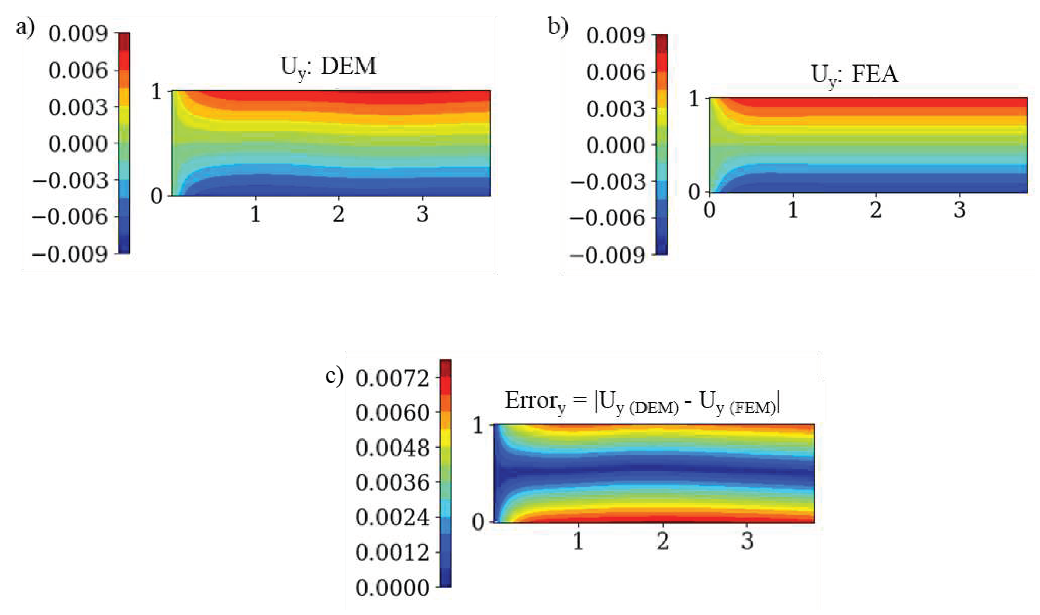
Figure 2.
ANN for DEM (Hyperparameters marked in blue).
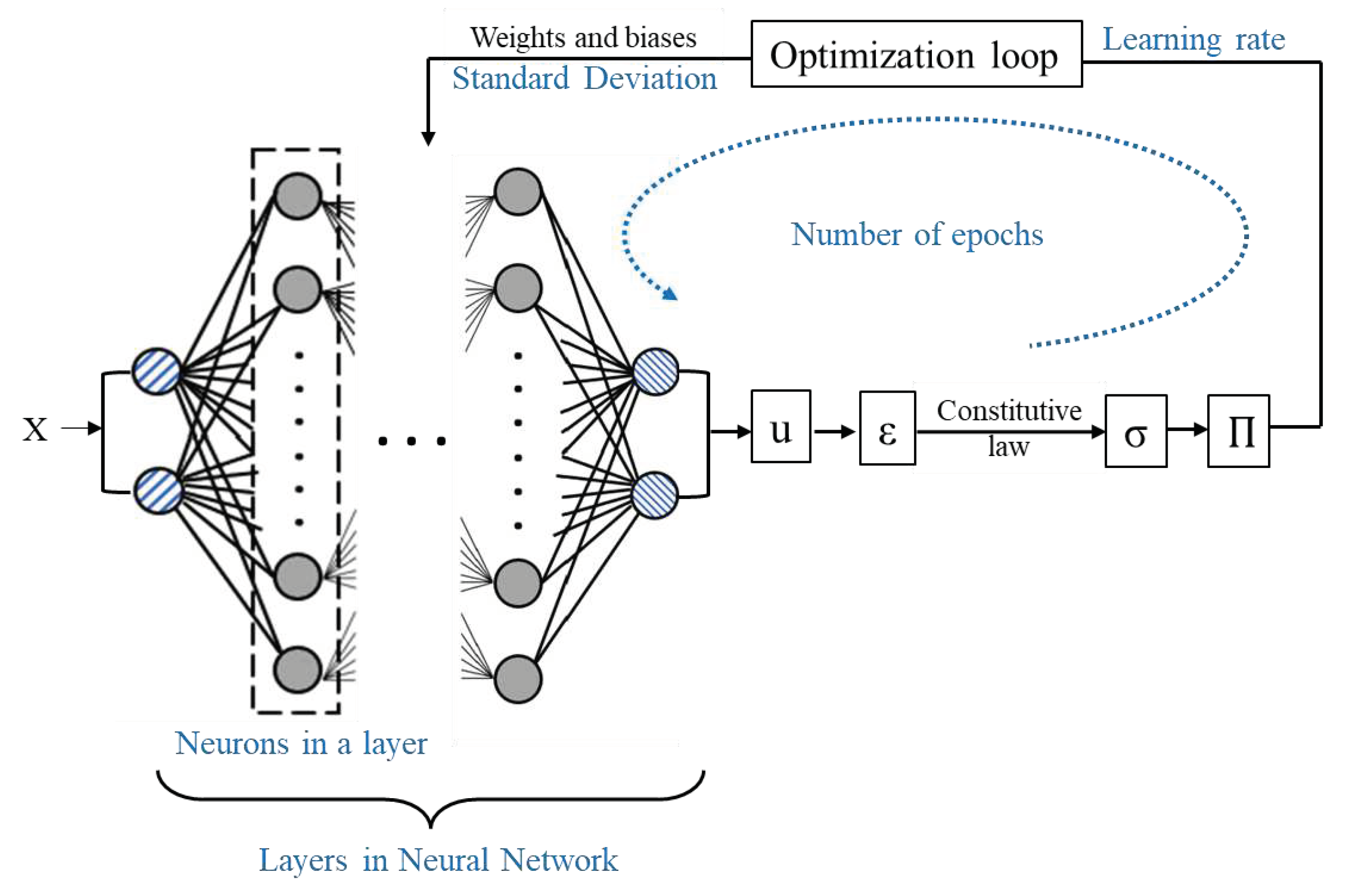
Figure 3.
Solid body with boundary conditions.
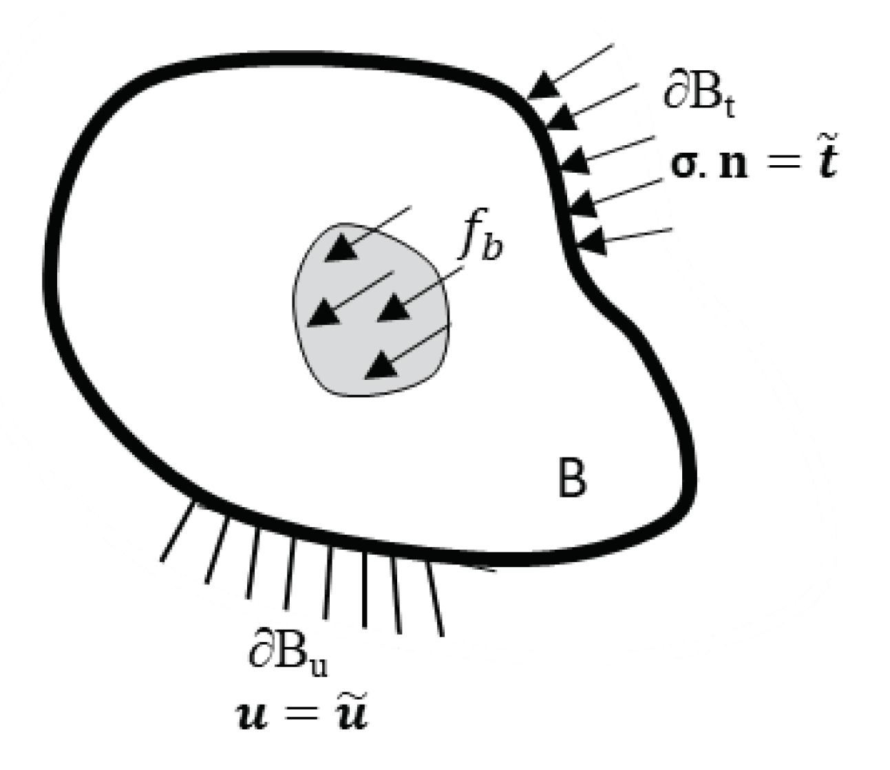
Figure 4.
Fourier feature mapping in the MLP.
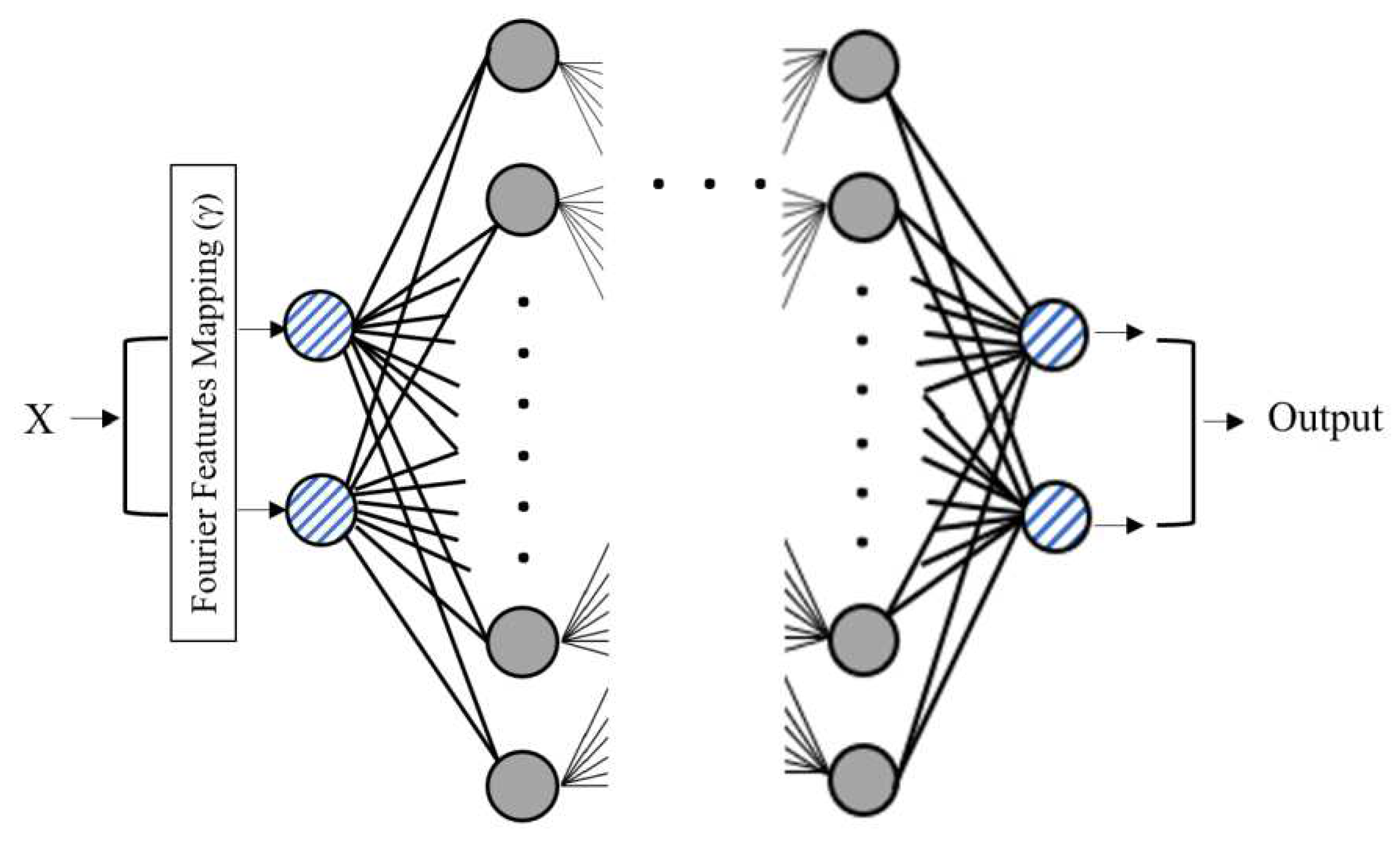
Figure 5.
Modified deep energy method.
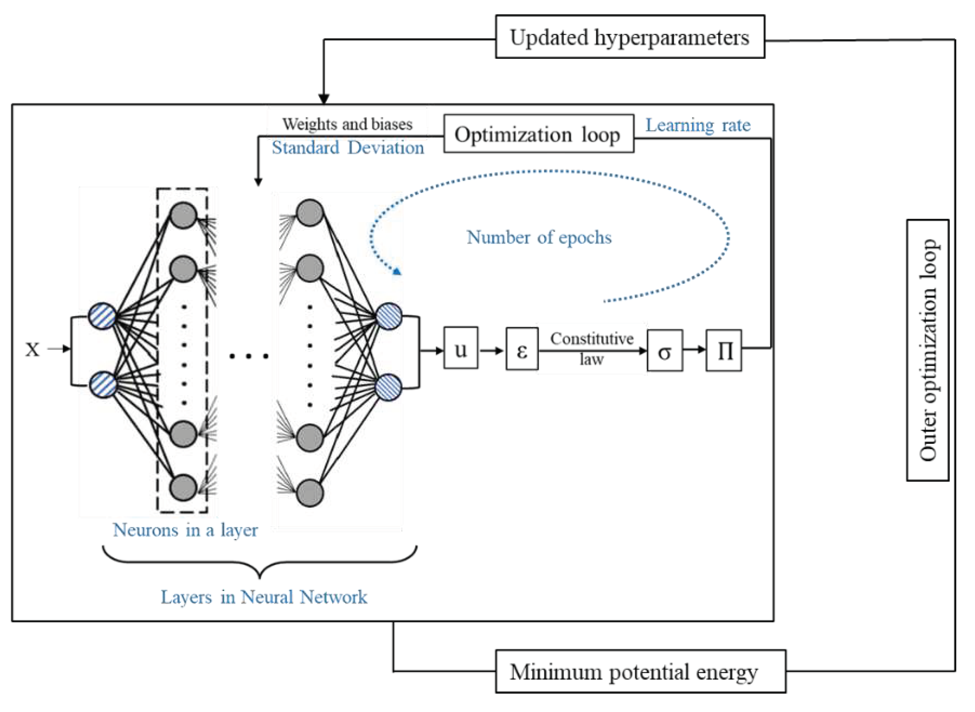
Figure 6.
Algorithm for hyperparameter tuning.
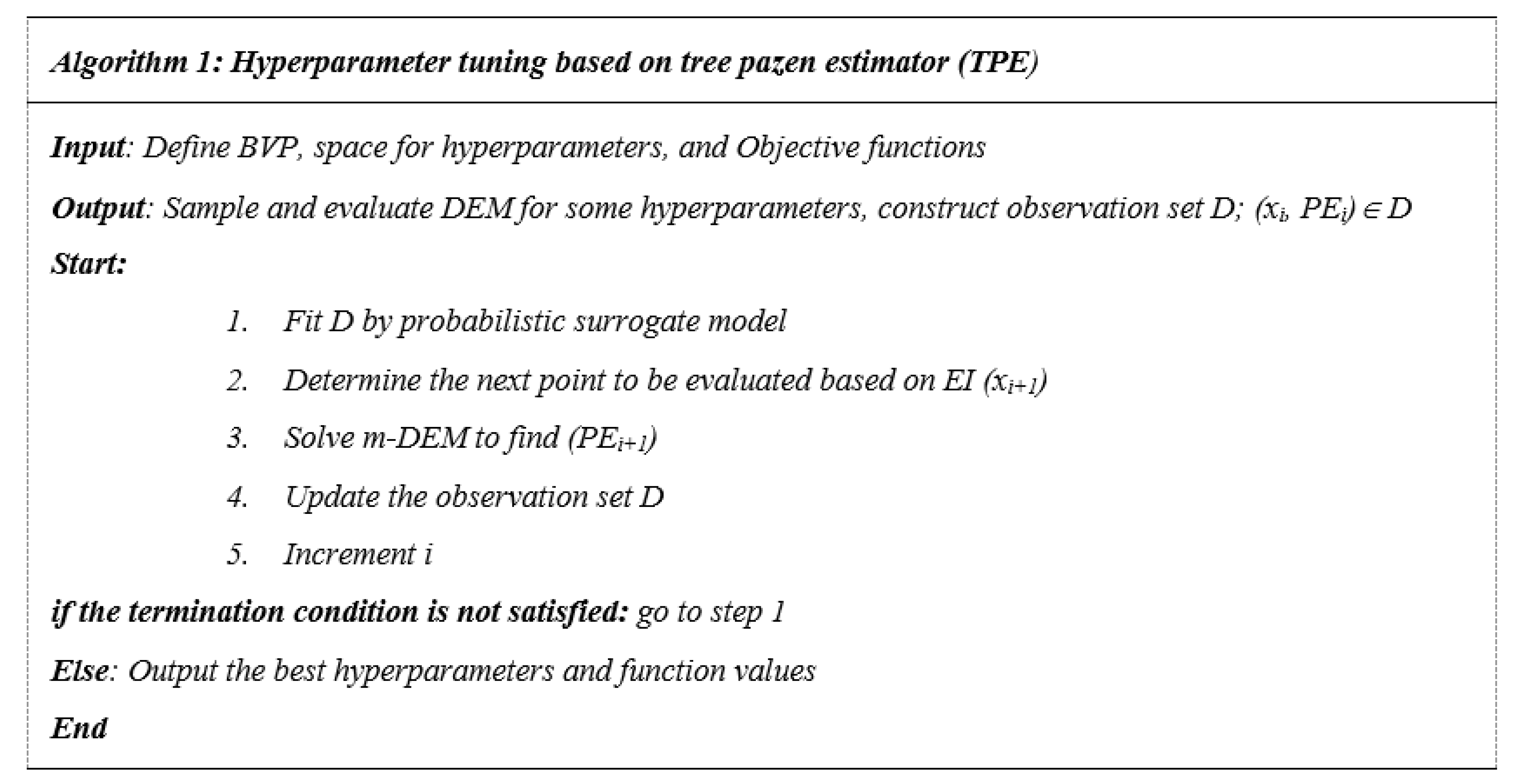
Figure 7.
Plate geometry and applied boundary conditions.
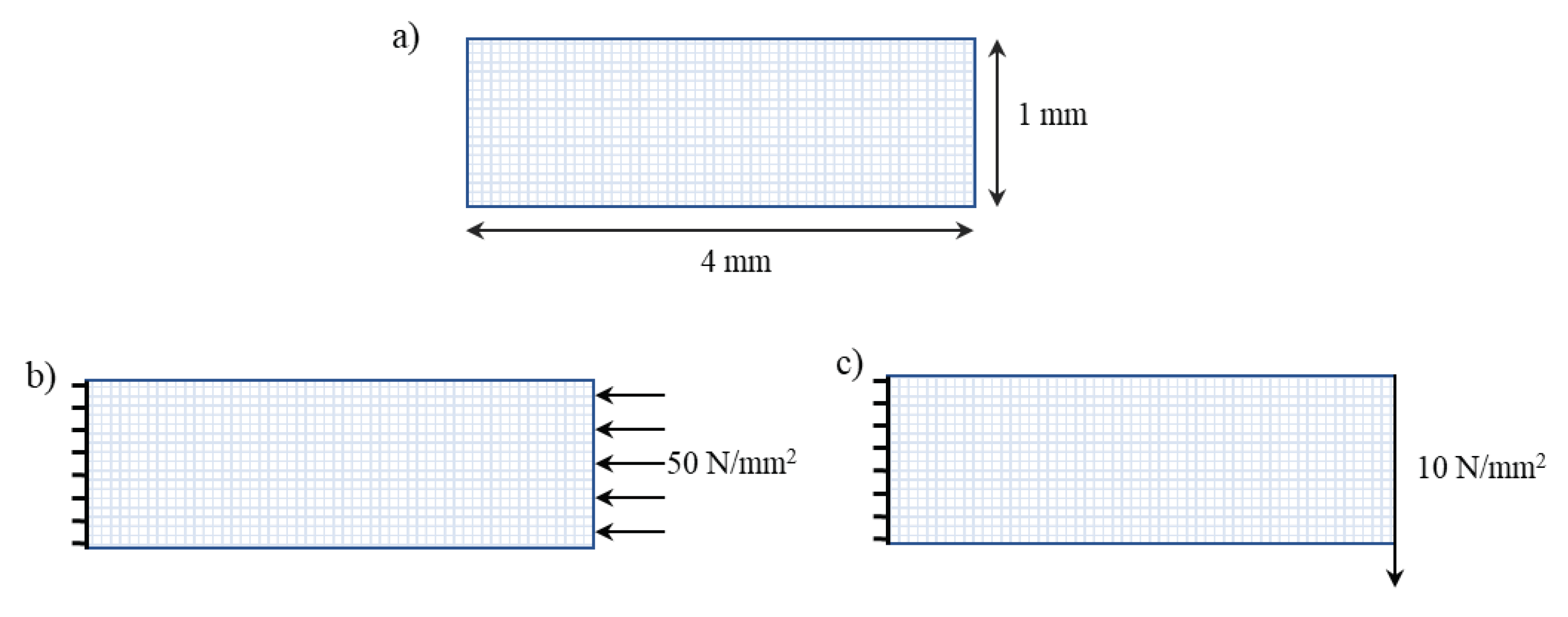
Figure 8.
Main effects plot.
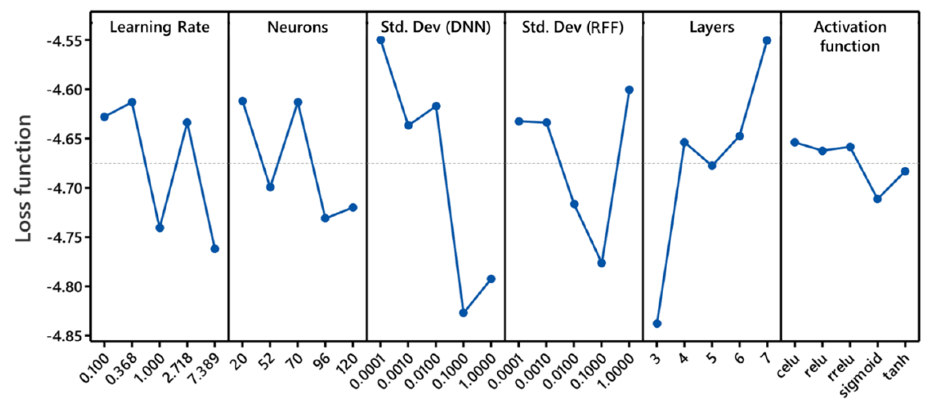
Figure 9.
Interactions plot.

Figure 10.
Anderson-Darling test for loss function.
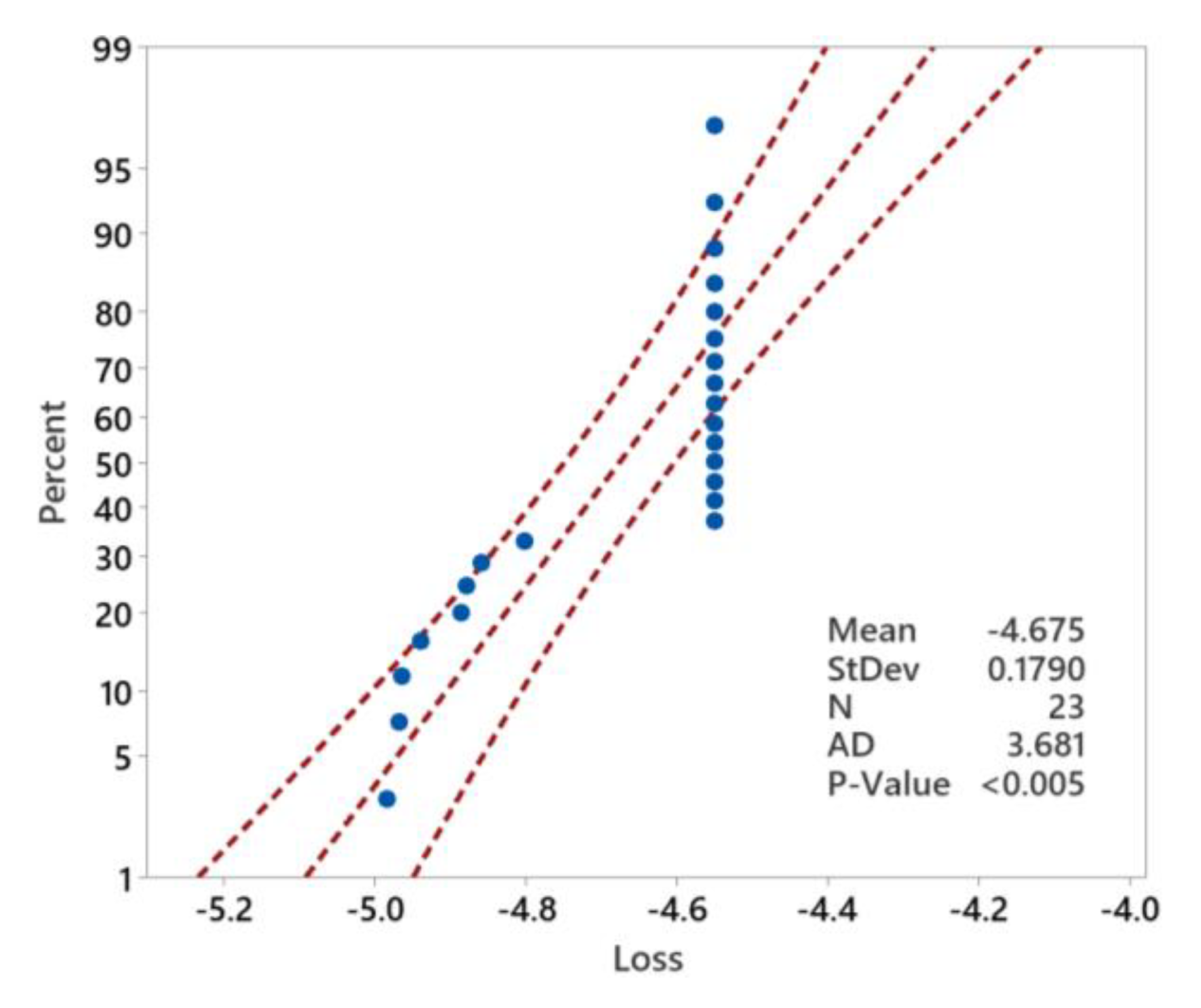
Figure 11.
Variation of the loss function (PE) with 500 randomly selected combinations of hyperparameters.
Figure 11.
Variation of the loss function (PE) with 500 randomly selected combinations of hyperparameters.
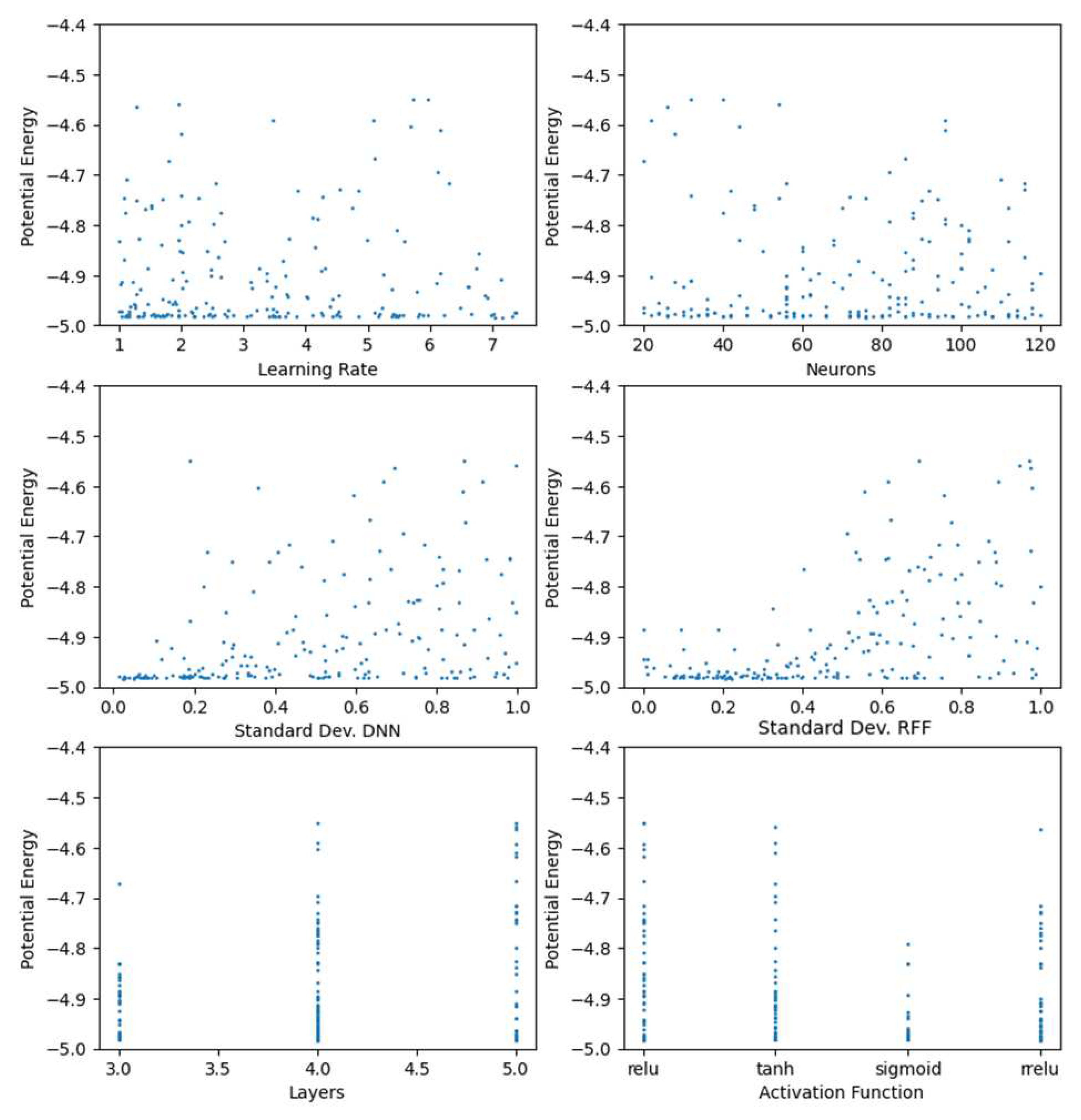
Figure 12.
Displacement in the y-direction and a) loss function of -4.83355, b) loss function of -4.97902.
Figure 12.
Displacement in the y-direction and a) loss function of -4.83355, b) loss function of -4.97902.
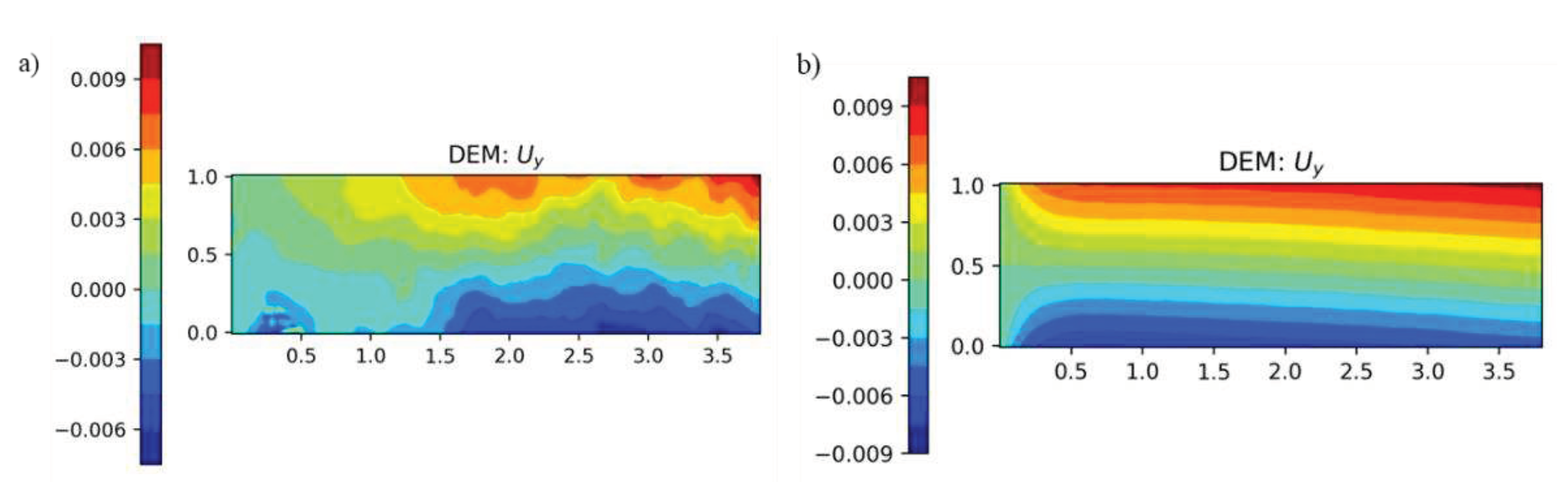
Figure 13.
Positions of training points for all load cases studied in Section 4.
Figure 13.
Positions of training points for all load cases studied in Section 4.
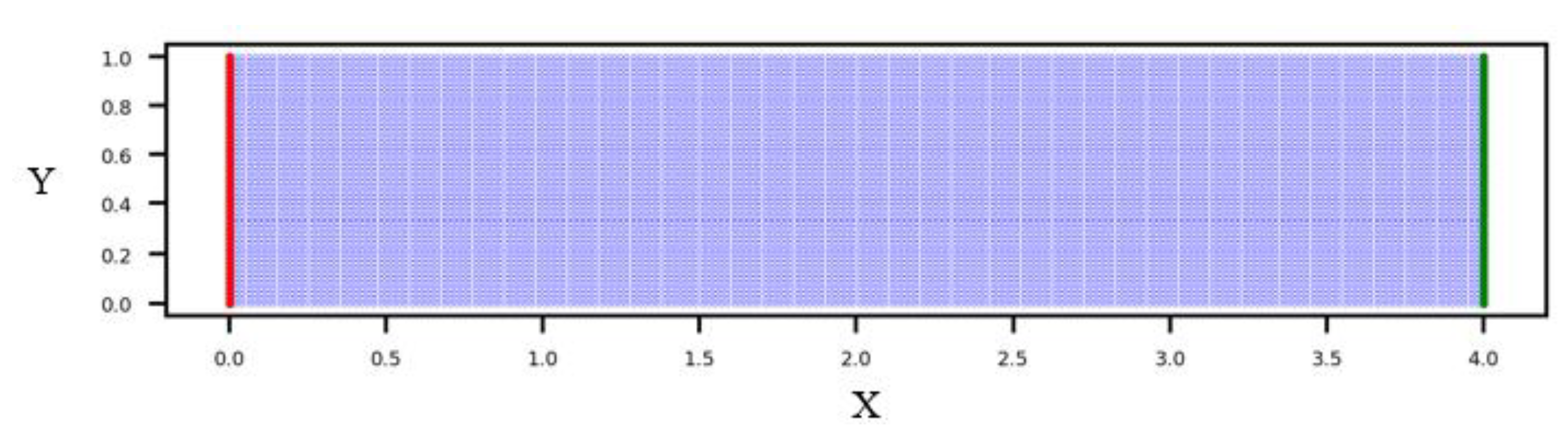
Figure 14.
Predicted displacements under compressive (a-b), tensile (c-d), and bending (e-f) loads.

Figure 15.
Error in predicted displacements under compressive (a-b), tensile (c-d), and bending (e-f) loads.
Figure 15.
Error in predicted displacements under compressive (a-b), tensile (c-d), and bending (e-f) loads.
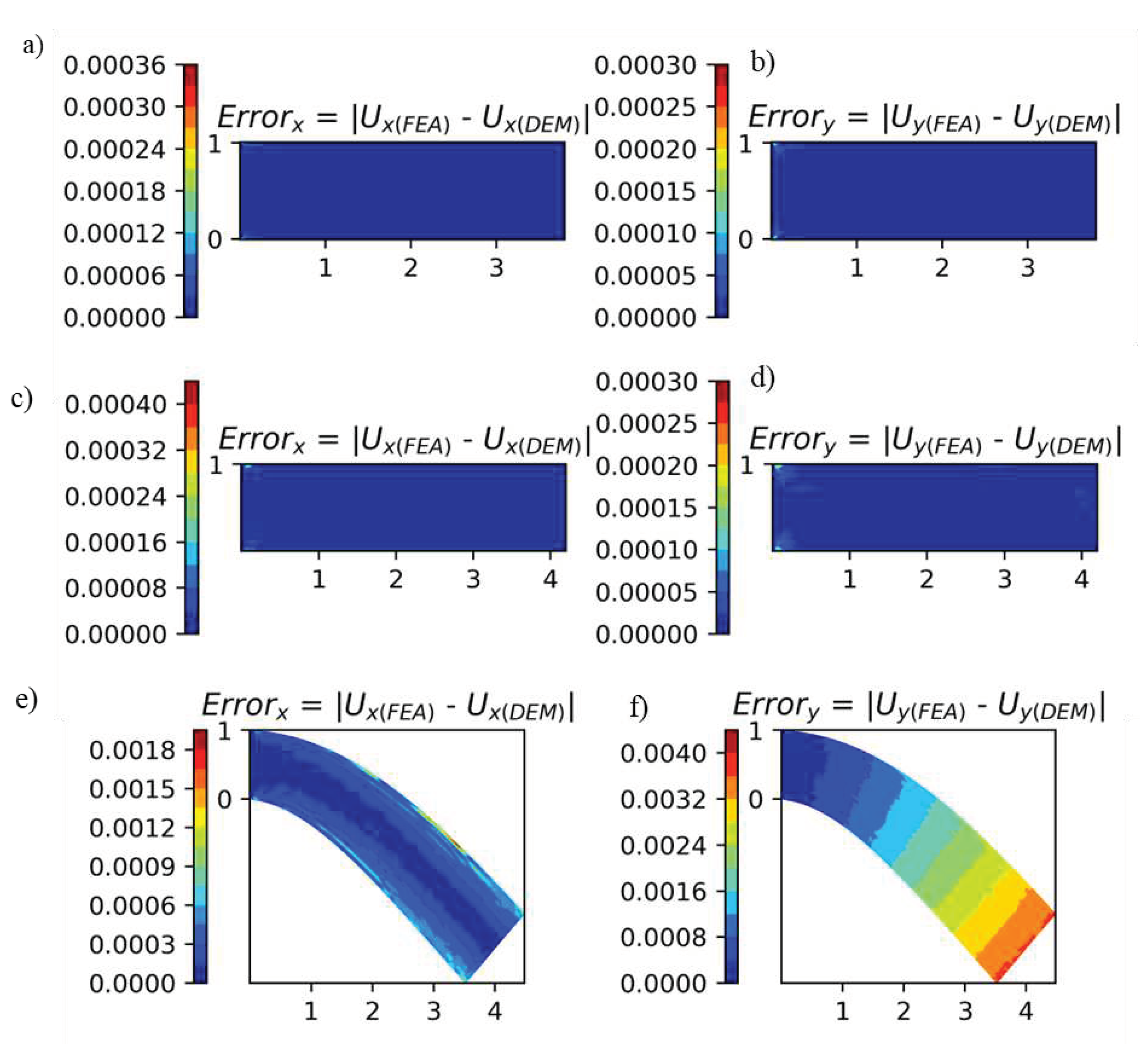
Figure 16.
Predicted displacement and error in y-direction for 200x50 and 100x100 discretizations.
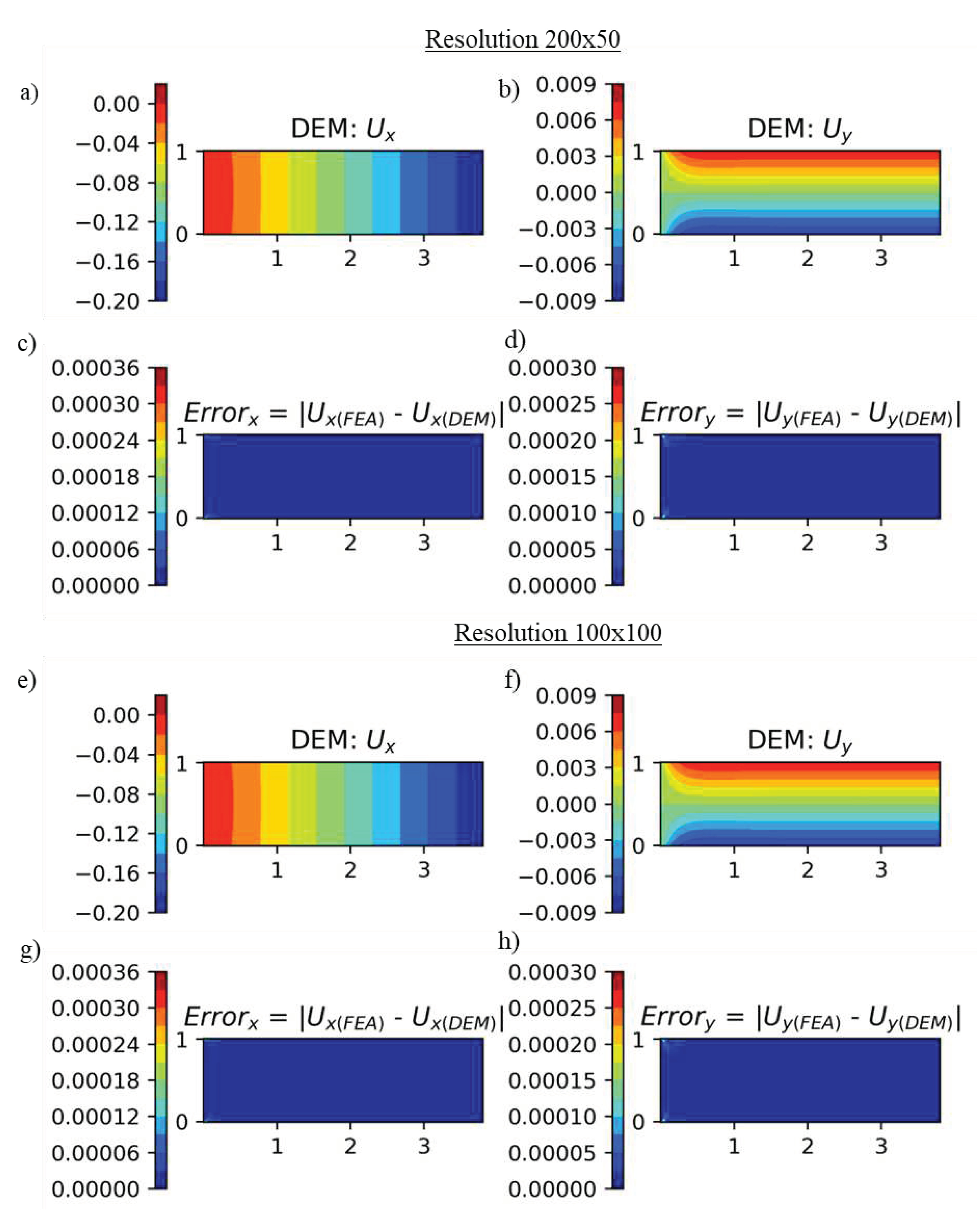
Figure 17.
a) 1mm x 1mm plate subjected to compressive loads, b) Training points used for DEM.
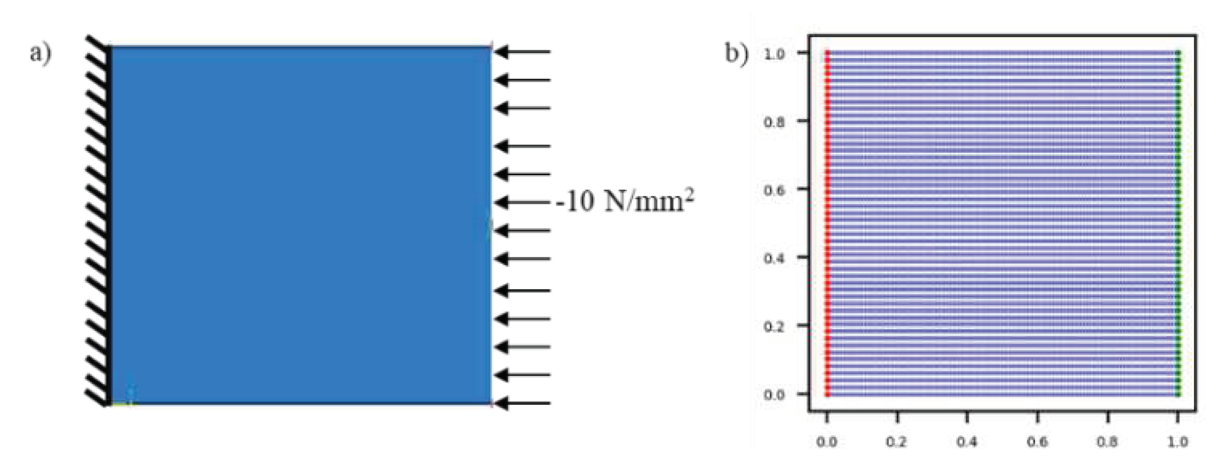
Figure 18.
a-b) displacements obtained predicted from DEM, c-d) displacements obtained from FEA, e-f) error in displacements.
Figure 18.
a-b) displacements obtained predicted from DEM, c-d) displacements obtained from FEA, e-f) error in displacements.
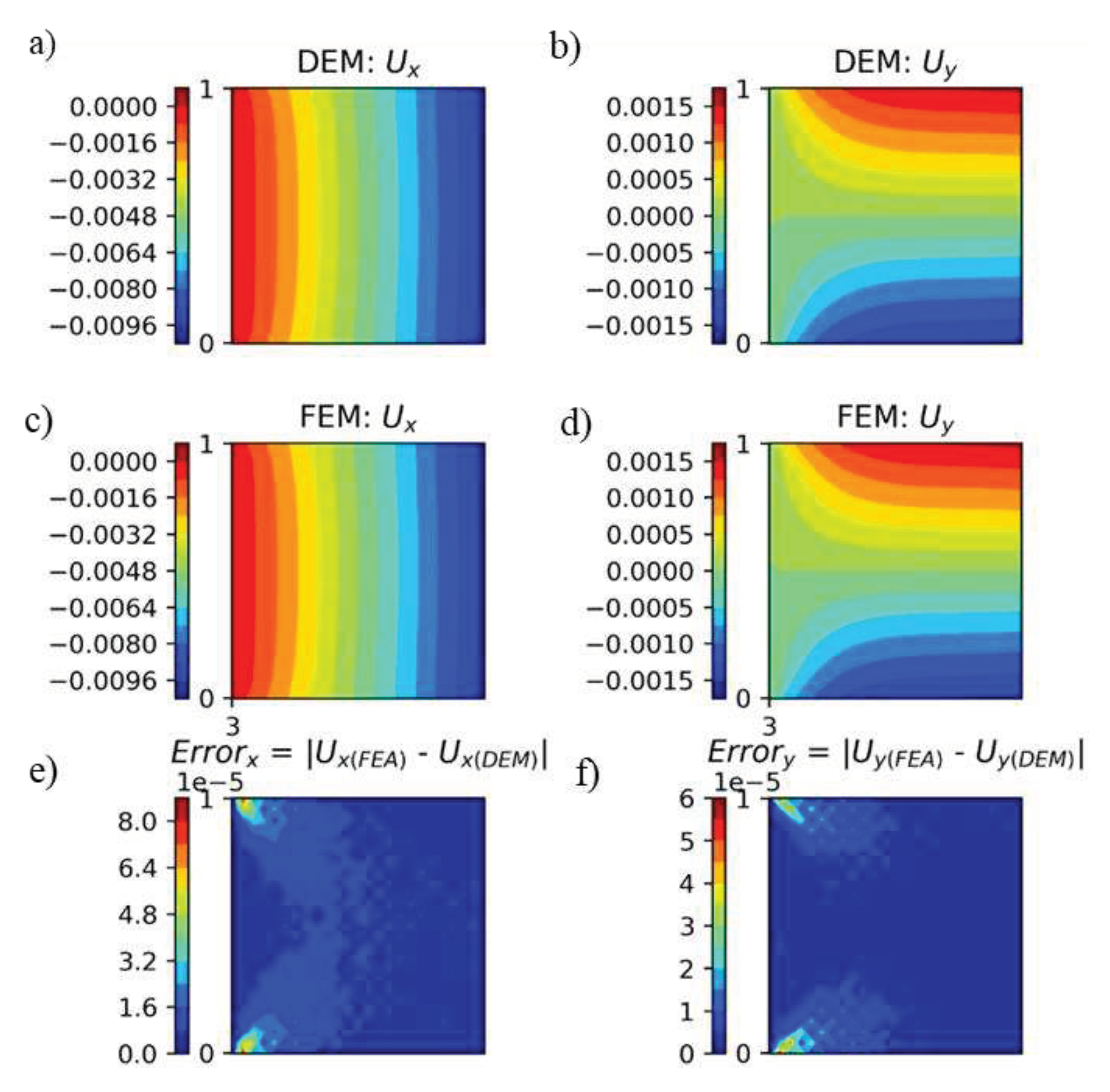
Figure 19.
a-b) displacements obtained for 1 mm x 1 mm plate when DEM model is trained for a plate of dimensions 4 mm x 1 mm, c-d) displacements obtained from FEA, e-f) error in displacements.
Figure 19.
a-b) displacements obtained for 1 mm x 1 mm plate when DEM model is trained for a plate of dimensions 4 mm x 1 mm, c-d) displacements obtained from FEA, e-f) error in displacements.
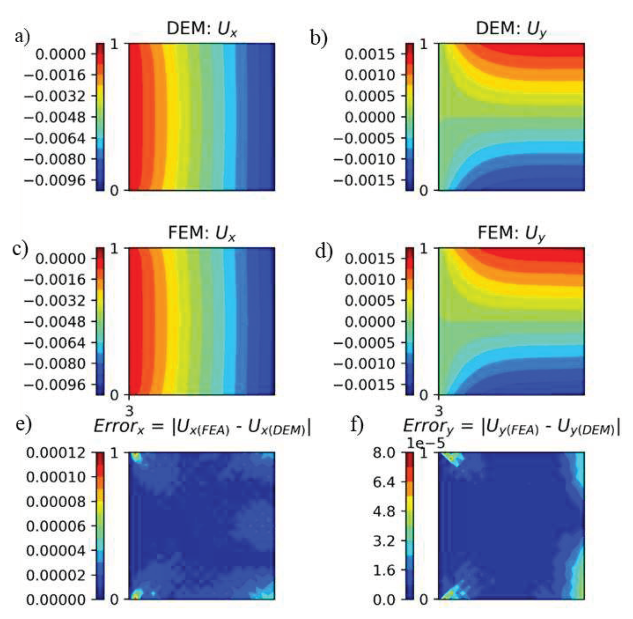
Figure 20.
a) Boundary conditions of the plate under localized traction. b) Training points used for DEM.
Figure 20.
a) Boundary conditions of the plate under localized traction. b) Training points used for DEM.
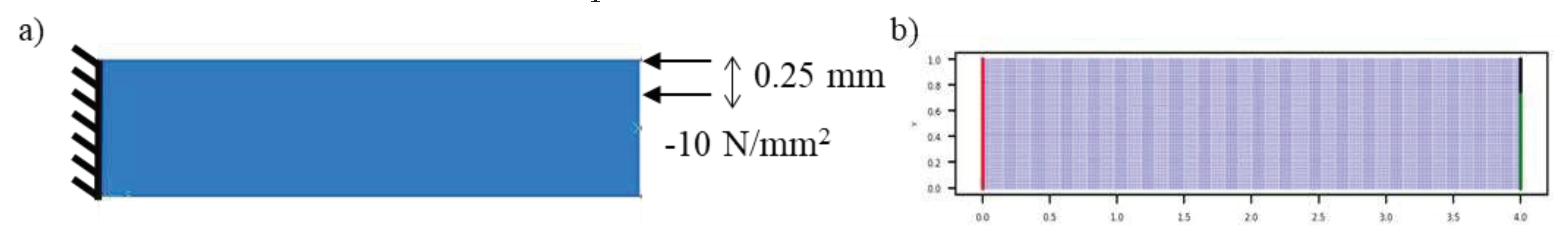
Figure 21.
a-b) displacements predicted from DEM, c-d) displacements obtained from FEA, and e-f) error in displacements for localized traction.
Figure 21.
a-b) displacements predicted from DEM, c-d) displacements obtained from FEA, and e-f) error in displacements for localized traction.
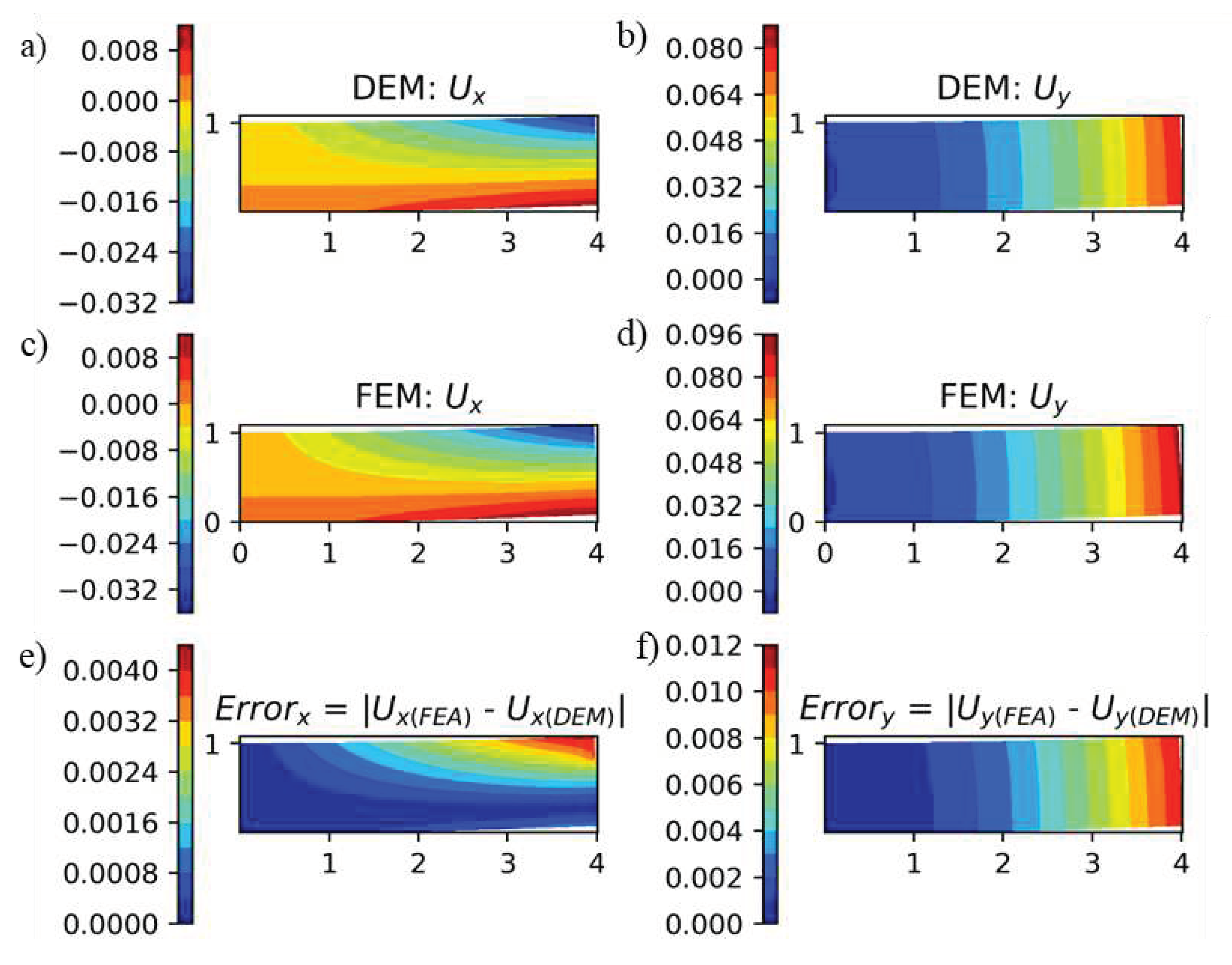
Figure 22.
Density distribution. The passive elements are shown in black while the elements while the active elements are in white.
Figure 22.
Density distribution. The passive elements are shown in black while the elements while the active elements are in white.
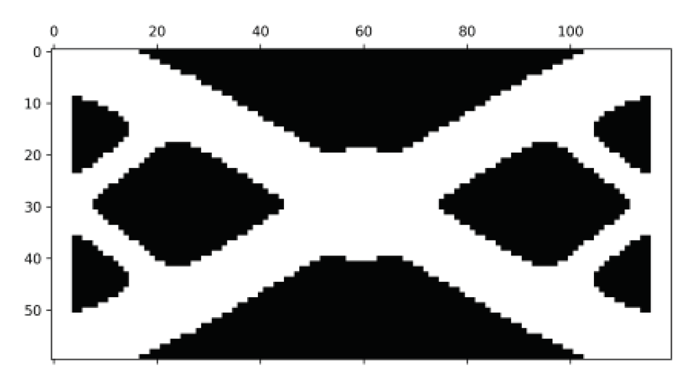
Figure 23.
a-b) displacements obtained predicted from DEM, c-d) displacements obtained from FEA, and e-f) error in displacements.
Figure 23.
a-b) displacements obtained predicted from DEM, c-d) displacements obtained from FEA, and e-f) error in displacements.
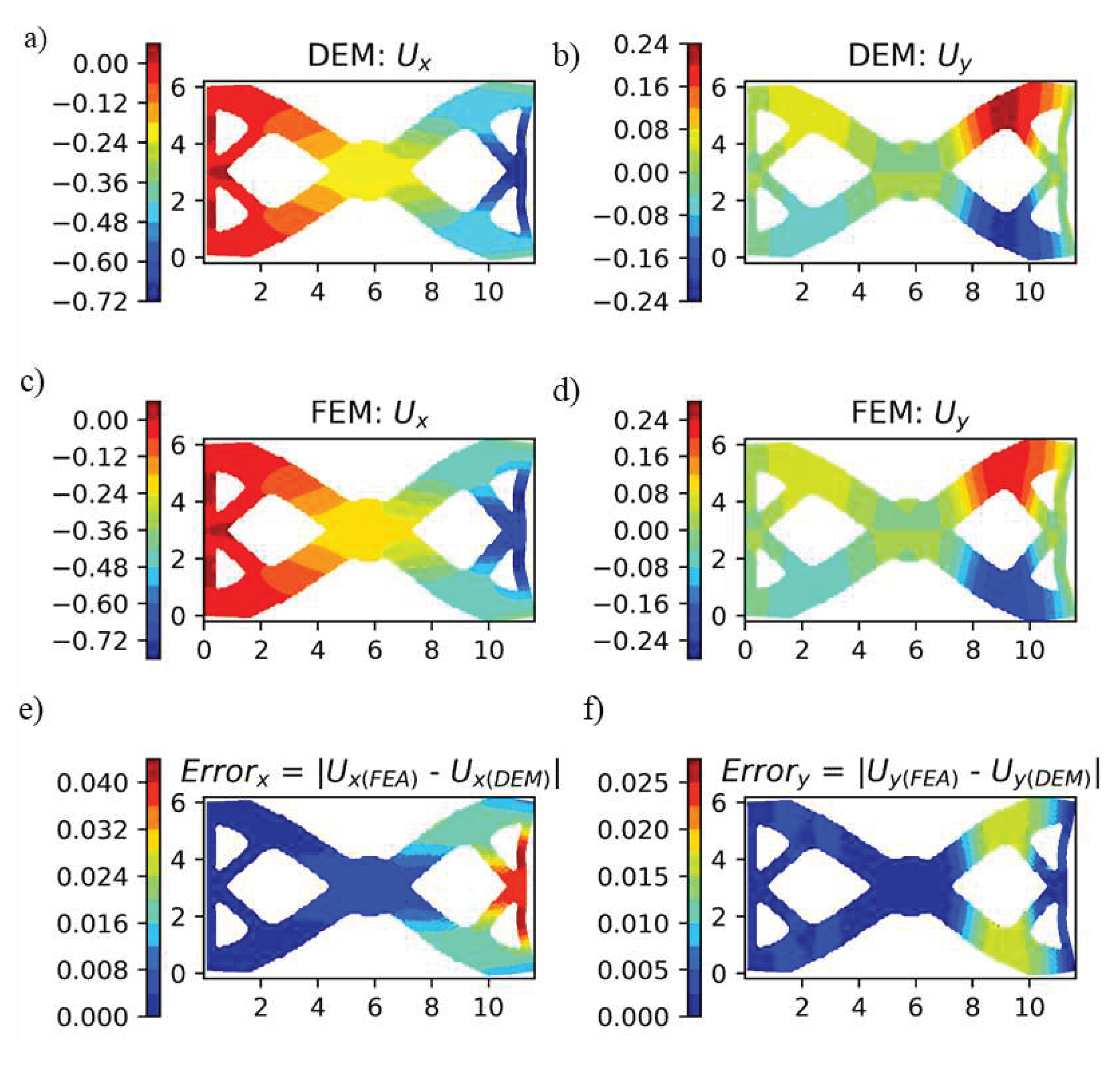
Figure 24.
a-b) displacements obtained predicted from DEM without RFF mapping, c-d) displacements obtained from FEA, and e-f) error in displacements.
Figure 24.
a-b) displacements obtained predicted from DEM without RFF mapping, c-d) displacements obtained from FEA, and e-f) error in displacements.
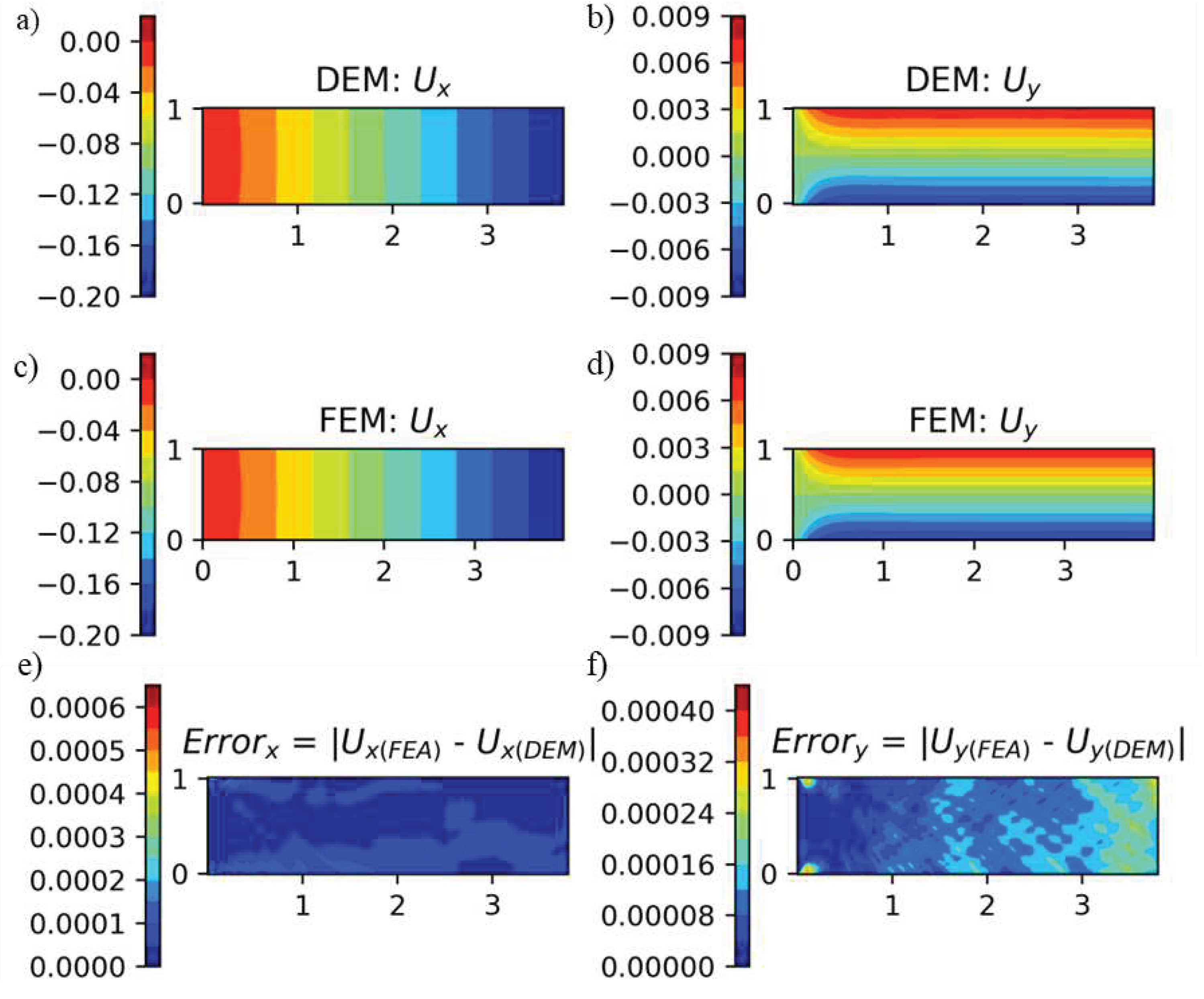
Figure 25.
a-b) displacements obtained predicted from DEM without RFF mapping under bending load, c-d) displacements obtained from FEA, and e-f) error in displacements.
Figure 25.
a-b) displacements obtained predicted from DEM without RFF mapping under bending load, c-d) displacements obtained from FEA, and e-f) error in displacements.

Figure 26.
a-b) displacements obtained predicted from DEM without RFF mapping under compressive load, c-d) displacements obtained from FEA, and e-f) error in displacements.
Figure 26.
a-b) displacements obtained predicted from DEM without RFF mapping under compressive load, c-d) displacements obtained from FEA, and e-f) error in displacements.
Disclaimer/Publisher’s Note: The statements, opinions and data contained in all publications are solely those of the individual author(s) and contributor(s) and not of MDPI and/or the editor(s). MDPI and/or the editor(s) disclaim responsibility for any injury to people or property resulting from any ideas, methods, instructions or products referred to in the content. |
© 2023 by the authors. Licensee MDPI, Basel, Switzerland. This article is an open access article distributed under the terms and conditions of the Creative Commons Attribution (CC BY) license (http://creativecommons.org/licenses/by/4.0/).
Copyright: This open access article is published under a Creative Commons CC BY 4.0 license, which permit the free download, distribution, and reuse, provided that the author and preprint are cited in any reuse.


