Ultra-Sparse Network Advantage in Deep Learning via Cannistraci-Hebb Brain-Inspired Training With Hyperbolic Meta-Deep Community-Layered Epitopology

Preprint

Article

Ultra-Sparse Network Advantage in Deep Learning via Cannistraci-Hebb Brain-Inspired Training With Hyperbolic Meta-Deep Community-Layered Epitopology

Altmetrics

Downloads

564

Views

668

Comments

Yingtao Zhang,Jialin Zhao,Wenjing Wu,Alessandro Muscoloni,

Carlo Vittorio Cannistraci^*

Yingtao Zhang,Jialin Zhao,Wenjing Wu,Alessandro Muscoloni,

Carlo Vittorio Cannistraci^*

This version is not peer-reviewed

Submitted:

26 October 2023

Posted:

30 October 2023

Read the latest preprint version here

Alerts

Abstract

Sparse training (ST) aims to ameliorate deep learning by replacing fully connected artificial neural networks (ANNs) with sparse or ultra-sparse ones, such as brain networks are, therefore it might benefit to borrow brain-inspired learning paradigms from complex network intelligence theory. Here, we launch the ultrasparse advantage challenge, whose goal is to offer evidence on the extent to which ultra-sparse (around 1% connection retained) topologies can achieve any leaning advantage on fully connected. Epitopological learning is a field of network science and complex network intelligence that studies how to implement learning on complex networks by changing the shape of their connectivity structure (epitopological plasticity). One way to implement Epitopological (epi- means new) Learning is via link prediction: predicting the likelihood of nonobserved links to appear in the network. Cannistraci-Hebb learning theory inspired the CH3-L3 network automata rule for link prediction which is effective for general-purpose link prediction. Here, starting from CH3-L3 we propose Epitopological Sparse Meta-deep Learning (ESML) to apply Epitopological Learning to sparse training. In empirical experiments, we find that ESML learns ANNs with ultra-sparse hyperbolic (epi-)topology in which emerges a community layer organization that is meta-deep (meaning that each layer also has an internal depth due to powerlaw node hierarchy). Furthermore, we discover that ESML can in many cases automatically sparse the neurons during training (arriving even to 30% neurons left in hidden layers), this process of node dynamic removal is called percolation. Starting from this network science evidence, we design Cannistraci-Hebb training (CHT), a 4-step training methodology that put ESML at its heart. We conduct experiments on 6 datasets and 3 network structures (MLPs, VGG16, ResNet50) comparing CHT to dynamic sparse training SOTA algorithms and fully connected network. The results indicate that, with a mere 1% of links retained during training, CHT surpasses fully connected networks on VGG16 and ResNet50. This key finding is an evidence for ultra-sparse advantage and signs a milestone in deep learning. CHT acts akin to a gradient-free oracle which adopts CH3-L3 based epitopological learning to guide the placement of new links in the ultra-sparse network topology to facilitate sparse-weight gradient learning, and this in turn reduces the convergence time of ultra-sparse training. Finally, CHT offers first examples of parsimony dynamic sparse training because, in many datasets, it canretain network performance by percolating and significantly reducing the node network size.

Keywords:

Subject: Computer Science and Mathematics - Artificial Intelligence and Machine Learning

1. Introduction

The human brain can learn using sparse and ultra-sparse neural network topologies and spending few watts, while current artificial neural networks are mainly based on fully connected topologies. How to make profit from ultra-sparse brain-inspired principles to ameliorate deep learning is the question that we try to address in this study, where we launch the ultra-sparse advantage challenge: the goal is to offer evidence on the extent to which ultra-sparse (around 1% connection retained) topologies can achieve any leaning advantage on fully connected. The ultra-sparse advantage challenge is in line with the current research in AI, focusing on how to reduce the training burden of the models in order to increase its trade-off efficiency between training speed, performance, and model size.

There exist two popular methods known as pruning Frantar & Alistarh (2023); Hassibi et al. (1993); LeCun et al. (1989); Li & Louri (2021); Sun et al. (2023); Zhang et al. (2023a) and sparse training Evci et al. (2020); Lee et al. (2019); Mocanu et al. (2018); Yuan et al. (2021 2022); Zhang et al. (2022 2023b) which introduce sparsity into deep learning. However, there are fundamental differences between them. Pruning begins with a fully connected network and gradually eliminates connections, aiming to strike a balance between post-training inference speed and final performance. Sparse training methods initiate with a sparsely connected network, resulting in inherent sparsity in both the forward and backward processes during training. Consequently, the primary goal of sparse training methods is to find the equilibrium balance between training acceleration and final performance. Dynamic Sparse Training (DST) Evci et al. (2020); Mocanu et al. (2018); Yuan et al. (2021), a variant of sparse training, is always considered as the most efficient strategy due to its ability to dynamically evolve the network’s topology. However, it’s worth noting that many DST algorithms don’t solely rely on the intrinsic network sparsity throughout the training process. For instance, approaches like RigL Evci et al. (2020) leverage gradient information from missing links, making the network fully connected during the backpropagation phase. Similarly, OptG Zhang et al. (2022) introduces an extra super-mask, adding learnable parameters during training. These DST methods deviate from the core principle of sparse training, which aims to accelerate model training solely through the existing connections in the network. Integrating theories from topological network science, particularly those inspired by complex network intelligence theory designed for sparse topological scenarios, into DST could yield fascinating results.

Epitopological Learning (EL) Cannistraci (2018); Daminelli et al. (2015); Durán et al. (2017) is a field of network science inspired by the brain that explores how to implement learning on networks by changing the shape of their connectivity structure (epitopological plasticity). One approach to implement EL is via link prediction: predicting the existence likelihood of each non-observed link in a network. EL was developed alongside the Cannistraci-Hebb (CH) learning theory Cannistraci (2018); Daminelli et al. (2015); Durán et al. (2017) according to which: the sparse local-community organization of many complex networks (such as the brain ones) is coupled to a dynamic local Hebbian learning process and contains already in its mere structure enough information to partially predict how the connectivity will evolve during learning. CH3-L3 Muscoloni et al. (2020), one of the network automata rules under CH theory, is effective for general-purposed link prediction in bipartite networks. Building upon CH3-L3, we propose Epitopological Sparse Meta-deep Learning (ESML) to implement EL in evolving the topology of ANNs based on dynamic sparse training procedure. Finally, we design CH training (CHT), a 4-step training methodology that puts ESML at its heart, with the aim to enhance prediction performance. Empirical experiments are conducted across 6 datasets (MNIST, Fashion_MNIST, EMNIST, CIFAR10, CIFAR100, ImageNet2012) and 3 network structures (MLPs, VGG16, ResNet50), comparing CHT to dynamic sparse training SOTA algorithms and fully connected network. The results indicate that with a mere 1% of links retained during training, CHT surpasses fully connected networks on VGG16 and ResNet50. This key finding is an evidence for ultra-sparse advantage and signs a milestone in deep learning.

2. Related Work

2.1. Dynamic sparse training

The basic theoretical and mathematical notions of dynamic sparse training together with the several baseline and SOTA algorithms including SET Mocanu et al. (2018), MEST Yuan et al. (2021) and RigL Evci et al. (2020) - which we adopt for comparison in this study - are described in the Appendix A. We encourage readers who are not experts on this topic to take a glance at this section in Appendix to get familiar with the basic concepts before going forward and reading this article.

2.2. Epitopological Learning and Cannistraci-Hebb network automata theory for link prediction

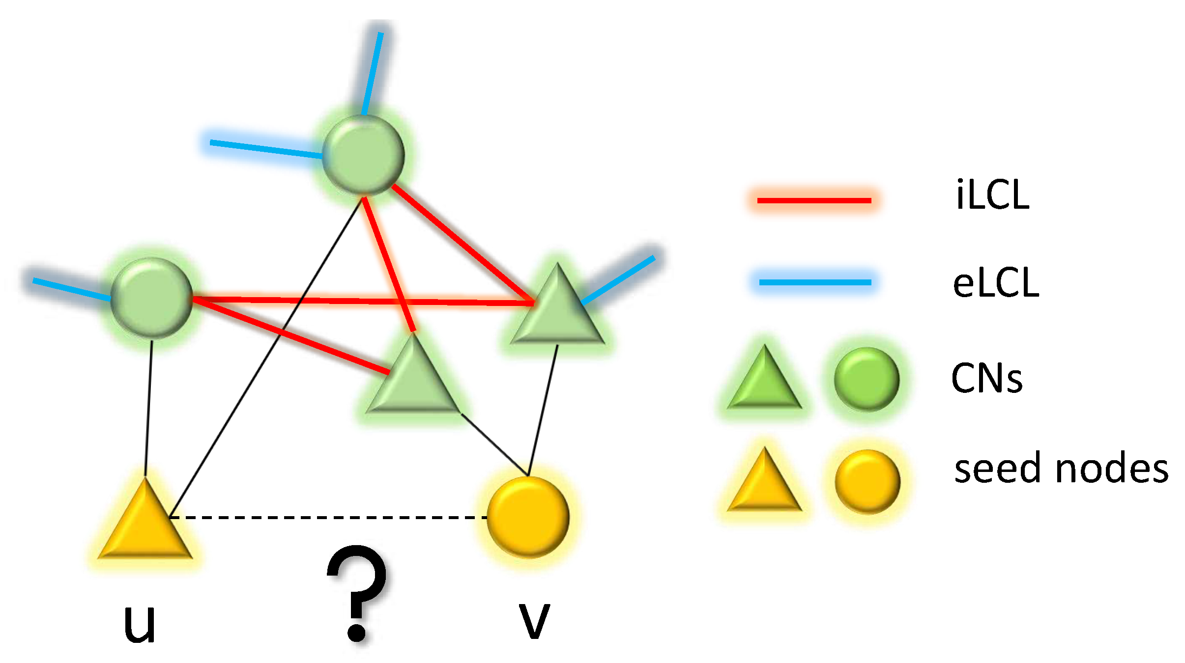
Drawn from neurobiology, Hebbian learning was introduced in 1949 Hebb (1949) and can be summarized in the axiom: “neurons that fire together wire together”. This could be interpreted in two ways: changing the synaptic weights (weight plasticity) and changing the shape of synaptic connectivity Cannistraci (2018); Cannistraci et al. (2013); Daminelli et al. (2015); Durán et al. (2017); Narula (2017). The latter is also called epitopological plasticity Cannistraci et al. (2013), because plasticity means “to change shape” and epitopological means “via a new topology”. Epitopological Learning (EL) Cannistraci (2018); Daminelli et al. (2015); Durán et al. (2017) is derived from this second interpretation of Hebbian learning, and studies how to implement learning on networks by changing the shape of their connectivity structure. One way to implement EL is via link prediction: predicting the existence likelihood of each nonobserved link in a network. In this study, we adopt CH3-L3 Muscoloni et al. (2020) as link predictor to regrow the new links during the DST process. CH3-L3 is one of the best and most robust performing network automata which is inside Cannistraci-Hebb (CH) theory Muscoloni et al. (2020) that can automatically evolve the network topology with the given structure. The rationale is that, in any complex network with local-community organization, cohort of nodes tend to be co-activated (fire together) and to learn by forming new connections between them (wire together) because they are topologically isolated in the same local community Muscoloni et al. (2020). This minimization of the external links induces a topological isolation of the local community, which is equivalent to form a barrier around the local community. The external barrier is fundamental to keep and reinforce the signaling in the local community inducing the formation of new links that participate to epitopological learning and plasticity. As illustrated in Fig A5, CH3-L3 accomplishes this task by incorporating external local community links (eLCLs) at the denominator of a formula that ensures common neighbors minimize their interactions outside the local community. CH3-L3 can be formalized as follows:

C H 3 - L 3 (u, v) = \sum_{z_{1}, z 2 \in l 3 (u, v)} \frac{1}{\sqrt{(1 + d e_{z_{1}}) * (1 + d e_{z_{2}})}},

(1)

where: u and v are the two seed nodes of the candidate interaction;

z_{1}, z_{2}

are the intermediate nodes on the considered path of length three which are seen as the common neighbors of u and v on the bipartite network;

d e_{z_{1}}

d e_{z_{2}}

are the respective number of external local community links of each common neighbor; and the summation is executed over all the paths of length three (l3) between the seed nodes u and v. The formula of

C H 3 - L n

is defined on path of any length, which adapts to any type of network organization Muscoloni et al. (2020). Here, we consider the length 3 paths of

C H 3 (C H 3 - L 3)

because the topological regrowth process is implemented on each ANN sandwich layer separately, which has bipartite network topology organization. And, bipartite topology is based on path of length 3 which displays a quadratic closure Daminelli et al. (2015). During the link prediction process, all the missing links in the network will be ranked based on scores generated by the

C H 3 - L 3

formula. A higher score suggests a higher probability of the link being present in the next stage of the network.

3. Epitopological sparse meta-deep learning and Cannistraci-Hebb training

3.1. Epitopological sparse meta-deep learning (ESML)

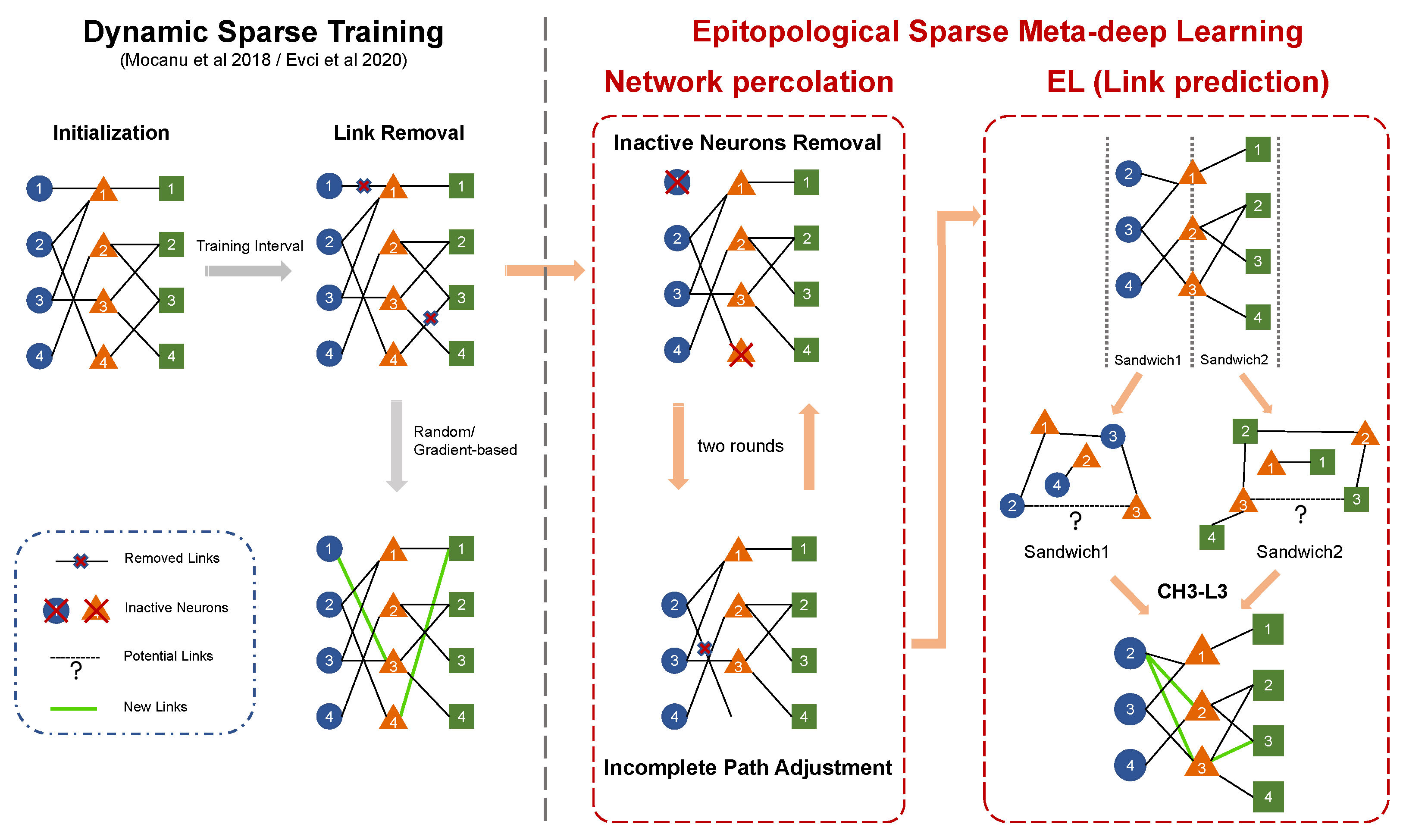
In this section, we propose epitopological sparse meta-deep Learning (ESML), which implements Epitopological Learning in the sparse deep learning ANN. In the standard dynamic sparse training (DST) process, as shown in Figure A3 (left side), there are three main steps: initialization, weight update, and network evolution. Network evolution consists of both link removal and link regrowth that in standard DST is random or gradient based Figure A3 (left side). ESML follows initially the same steps of standard DST link removal (Figure A3, left side), but then it does not implement the standard random or gradient based link growth. Indeed, ESML progresses with substantial improvements (Figure A3, right side): new additional node and link removal part (network percolation), and new regrowth part (EL via link prediction). ESML changes the perspective of training ANNs from weights to topology. As described in Section 2.2, Epitopological Learning is a general concept detailing how the learning process works by evolving the topology of the network. This topological evolution can take various forms, such as link removal and link regrowth. In this article, we explore the benefits that link regeneration within Epitopological Learning offers to dynamic sparse training. The topological update formula in this article is:

T^{n + 1} = T^{n} + L P_{T o p K} (T^{n}),

(2)

Where

T^{n}

represents the topology of the system at state n and

T^{n + 1}

represents the topology of the system at state

n + 1

L P

can be any link predictor, such as SPM Lü et al. (2015), CN Newman (2001), or CH3-L3 Muscoloni et al. (2020), to predict the likelihood and select the TopK missing links between pair of nodes in the network. Through an internal examination, we observed that CH3-L3 outperforms SPM and CN. Once the network percolation (Figure A3, right side), which removes inactive neurons and links, is finished, Epitopological Learning via link prediction is implemented to rank the missing links in the network. This is done by computing likelihood scores with the link predictor (CH3-L3 in this article) and then regrowing the same number of links as removed with higher scores. For the necessity to contain article’s length, the details of the two removal steps are offered in Appendix D. ESML can be repeated after any backpropagation. The most used update interval in dynamic sparse training can be in the middle of an epoch, after an epoch, or after any certain number of epochs. Thus, ESML is independent of the loss function and, after ESML predicts and adds the new links to the network topology, the backpropagation only transfers the gradient information through the existing links of topology

T

in an epoch. Our networks are ultra-sparse (1% connectivity) hence the gradient information navigates to find a minimum in a smaller dimensional space with respect to the fully connected. Compared to dense fully connected network backpropagation, in the link prediction-based dynamic sparse training, the gradient is computed considering only the existing links in the ultra-sparse topology. This means that if we preserve only 1% of the links, we only need to compute the gradients for those existing links and backpropagate them to the previous layers, which in principle could imply a 100 times training speed up.

3.2. Cannistraci-Hebb training

ESML is a methodology that can work better when the network has already formed some relevant structural features. For instance, the fact that in each layer the nodes display a hierarchical position is associated with their degree. Nodes with higher degrees are network hubs in the layer and therefore they have a higher hierarchy. This hierarchy is facilitated by a hyperbolic network geometry with power-law-like node degree distribution Cannistraci & Muscoloni (2022). In addition, the efficiency of the link predictor can be impaired by sparse random connectivity initialization. Therefore, we introduce below a strategy to initialize the sparse network topology and its weights. On the other hand, once the network topology has already stabilized (nodes removed and regrown are consistently similar), there may no longer be the necessity to perform ESML which could save time of evolution. Therefore, to address these concerns, we propose a novel 4-step training procedure named Cannistraci-Hebb training (CHT).

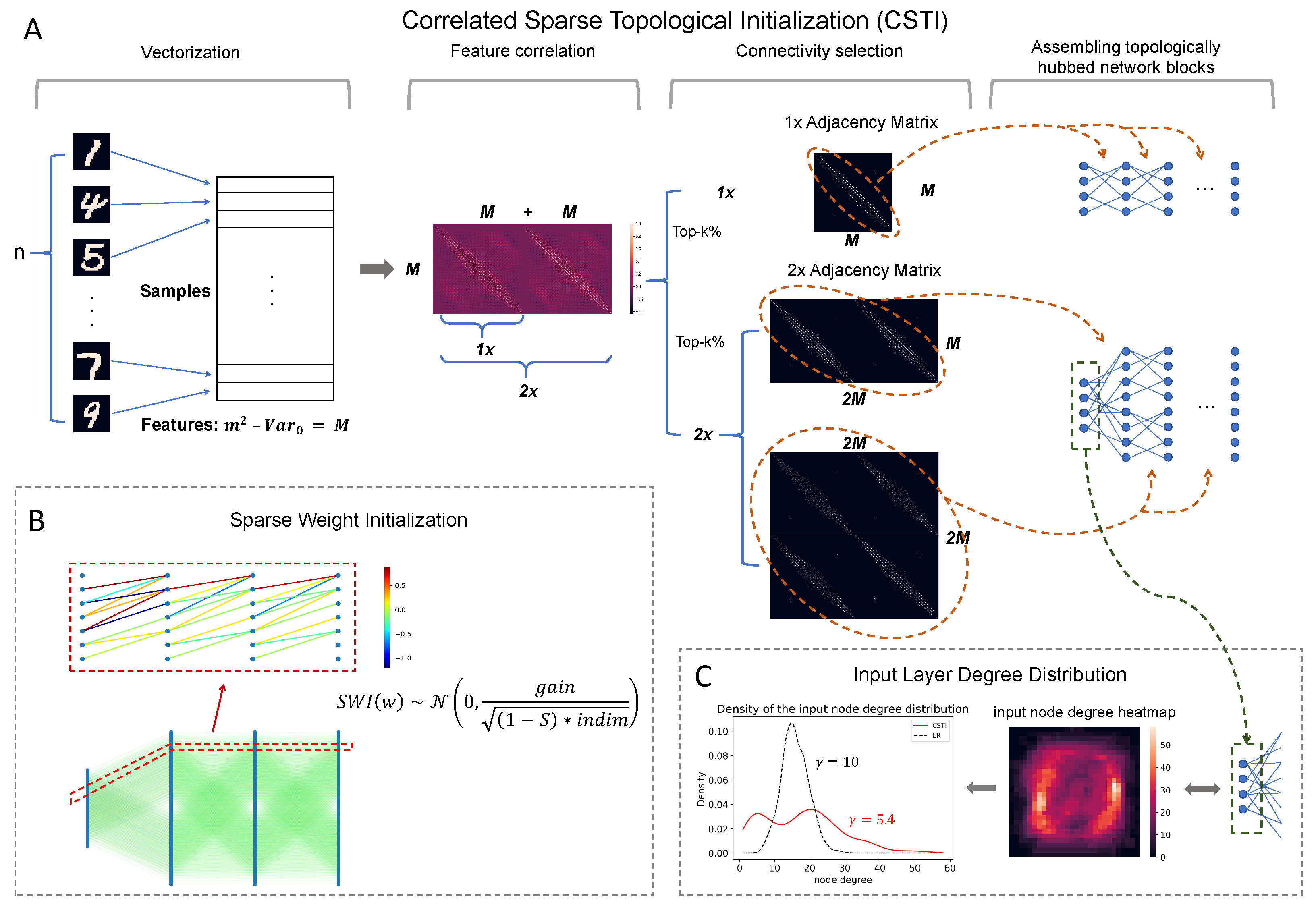
Correlated sparse topological initialization (CSTI): as shown in Figure A4, CSTI consists of 4 steps. 1) Vectorization: During the vectorization phase, we follow a specific procedure to construct a matrix of size $n \times M$ , where n represents the number of samples selected from the training set. M denotes the number of valid features, obtained by excluding features with zero variance ( $V a r_{0}$ ) among the selected samples. 2) Feature selection: Once we have this $n \times M$ matrix, we proceed with feature selection by calculating the Pearson Correlation for each feature. This step allows us to construct a correlation matrix. 3) Connectivity selection: Subsequently, we construct a sparse adjacency matrix, where the positions marked with “1" (represented as white in the heatmap plot of Figure A4) correspond to the top-k% values from the correlation matrix. The specific value of k depends on the desired sparsity level. This adjacency matrix plays a crucial role in defining the topology of each sandwich layer. The dimension of the hidden layer is determined by a scaling factor denoted as ‘×’. A scaling factor of $1 \times$ implies that the hidden layer’s dimension is equal to the input dimension, while a scaling factor of $2 \times$ indicates that the hidden layer’s dimension is twice the input dimension which allows the dimension of the hidden layer to be variable. In fact, since ESML can efficiently reduce the dimension of each layer, the hidden dimension can automatically reduce to the inferred size. 4) Assembling topologically hubbed network blocks: Finally, we implement this selected adjacency matrix to form our initialized topology for each sandwich layer.
Sparse Weight Initialization (SWI): In addition to the topological initialization, we also recognize the importance of weight initialization in the sparse network. The standard initialization methods such as Kaiming He et al. (2015) or Xavier Glorot & Bengio (2010) are designed to keep the variance of the values consistent across layers. However, these methods are not suitable for sparse network initialization since the variance is not consistent with the previous layer. To address this issue, we propose a method that can assign initial weights in any sparsity cases. SWI can also be extended to the fully connected network, in which case it becomes equivalent to Kaiming initialization. Here we provide the mathematical formula for SWI and in Appendix B, we provide the rationale that brought us to its definition.

$S W I (w) \sim N (0, σ^{2}), σ = \frac{g a i n}{\sqrt{(1 - S) * i n d i m}} .$

(3)

The value of gain varies for different activation functions. In this article, all the models use ReLU, where the gain is always $\sqrt{2}$ . S here denotes the desired sparsity and $i n d i m$ indicates the input dimension of each sandwich layer.
Epitopological prediction: This step corresponds to ESML (introduced in Section 3.1) but evolves the sparse topological structure starting from CSTI+SWI initialization rather than random.
Early stop and weight refinement: During the process of Epitological prediction, it is common to observe an overlap between the links that are removed and added, as shown in the last plot in Figure A2. After several rounds of topological evolution, the overlap rate can reach a high level, indicating that the network has achieved a relatively stable topological structure. In this case, ESML may continuously remove and add mostly the same links, which can slow down the training process. To solve this problem, we introduce an early stop mechanism for each sandwich layer. When the overlap rate between the removal and regrown links reaches a certain threshold (we use a significant level of 90%), we stop the epitopological prediction for that layer. Once all the sandwich layers have reached the early stopping condition, the model starts to focus on learning and refining the weights using the obtained network structure.

4. Results

4.1. Setup

In this section, we begin by presenting experimental results and network measurement analyses for ESML and SET Mocanu et al. (2018) across three datasets (MNIST LeCun et al. (1998), Fashion_MNIST Xiao et al. (2017), EMNIST Cohen et al. (2017)) using MLPs, and two datasets (CIFAR10 Krizhevsky (2009), CIFAR100 Krizhevsky (2009)) with VGG16 Simonyan & Zisserman (2014). CH3-L3 is chosen as the representative link predictor for ESML. Then, to further enhance the performance of ESML, we introduce a 4-step training methodology termed CHT. We present our comparative analysis of CHT on VGG16 with CIFAR10 and CIFAR100 and on ResNet50 He et al. (2016) with ImageNet2012 Russakovsky et al. (2015). The models employing dynamic sparse training in this section adopt the following network structures: 1) A 3-layer MLP; 2) The final three fully connected layers (excluding the last layer) of VGG16; 3) The final three fully connected layers (excluding the last layer) of ResNet50. It’s noteworthy that the default configuration for ResNet50 comprises just one fully connected layer. We expanded this to three layers to allow the implementation of dynamic sparse training. All experiments are conducted using three random seeds (except ResNet50), and a consistent set of hyperparameters is applied across all methods. Comprehensive hyperparameter details are available in Appendix L.1, where we also report information on hidden dimension, baseline methods, and sparsity in Appendix H.

4.2. Results for ESML and Network analysis of epitopological-based link regrown

4.2.1. ESML prediction performance

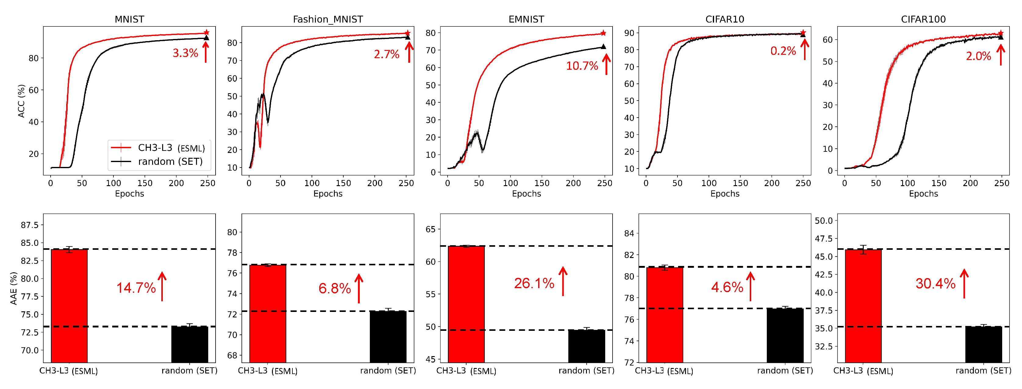
In this subsection, we aim to investigate the effectiveness of ESML from a network science perspective. We utilize the framework of ESML and compare CH3-L3 (the adopted topological link predictor) with randomly assigning new links (which is the regrown method of SET Mocanu et al. (2018)). Figure 1 compares the performance of CH3-L3 (ESML) and random (SET). The first row shows the accuracy curves of each algorithm and on the upper right corner of each panel, we mark the accuracy improvement at the 250th epoch. The second row of Figure 1 shows the area across the epochs (AAE), which reflects the learning speed of each algorithm. The computation and explanation of AAE can be found in the Appendix I. Based on the results of the accuracy curve and AAE values, ESML (CH3-L3) outperforms SET (random) on all the datasets, demonstrating that the proposed epitopological learning method is effective in identifying lottery tickets, and the CH theory is boosting deep learning.

4.2.2. Network Analysis

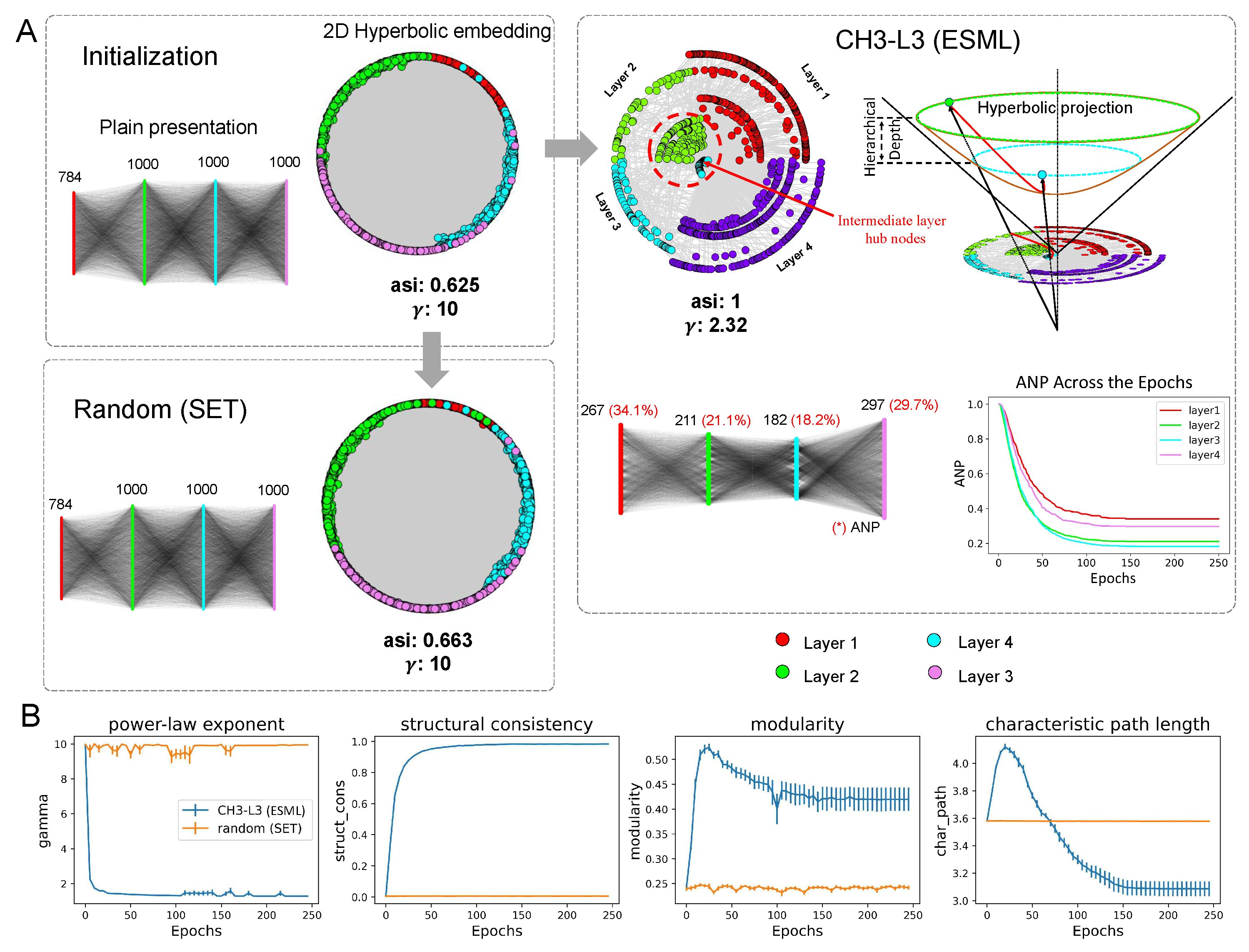
Figure 2A provides evidence that the sparse network trained with ESML can automatically percolate the network to a significantly smaller size and form a hyperbolic network with community organization. The example network structure of EMNIST dataset on MLP is presented, where each block shows a plain representation and a hyperbolic representation of each network at the initial (that is common) and the final epoch status (that is random (SET) or CH3-L3 (ESML)).

Network percolation.

The plain representation of the ESML block in Figure 2A shows that each layer of the network has been percolated to a small size, especially the middle two hidden layers where the active neuron post-percolation rate (ANP) has been reduced to less than 20%. This indicates that the network trained by ESML can achieve better performance with significantly fewer active neurons, and that the size of the hidden layers can be automatically learned by the topological evolution of ESML. ANP is particularly significant in deep learning because neural networks often have a large number of redundant neurons that do not contribute significantly to the model’s performance. Moreover, we present the analysis of the ANP reduction throughout the epochs within the ESML blocks/sandwiches. From our results, it is evident that the ANP diminishes to a significantly low level after approximately 50 epochs. This finding highlights the efficient network percolation capability of ESML, while in the meantime it suggests that a prolonged network evolution may not be necessary for ESML, as the network stabilizes within a few epochs, indicating its rapid convergence. 1

Hyperbolic hierarchical organization.

Furthermore, we perform coalescent embedding Cacciola et al. (2017) of each network in Figure 2A into the hyperbolic space, where the radial coordinates are associated with node degree hierarchical power-law-like distribution and the angular coordinates with geometrical proximity of the nodes in the latent space. This means that the typical tree-like structure of the hyperbolic network emerges if the node degree distribution is power law (gamma exponent of the power law distribution

γ \leq 3

Cannistraci & Muscoloni (2022)). Indeed, the more power law is the network, the more the nodes migrated towards the center of the hyperbolic 2D representation, and the more the network displays a hierarchical hyperbolic structure.

Hyperbolic community organization.

Surprisingly, we found that the network formed by CH3-L3 finally (at last epochs 250) becomes a hyperbolic power law (

γ

=2.32) network with hyperbolic community organization (angular separability index,

A S I = 1

, indicates a perfect angular separability of the community formed by each layer Muscoloni Cannistraci (2019)), while the others (initial and random at 250epochs) do not display either power law (

γ

=10) topology with latent hyperbolic geometry or crystal-clear community organization (ASI around 0.6 denotes a substantial presence of aberration in the community organization Muscoloni & Cannistraci (2019)). Community organization is a fundamental mesoscale structure of real complex networks Alessandro & Vittorio (2018); Muscoloni & Cannistraci (2018), such as biological and socioeconomical Xu et al. (2020). For instance, brain networks Cacciola et al. (2017) and maritime networks Xu et al. (2020) display distinctive community structure that is fundamental to facilitate diversified functional processing in each community separately and global sharing to integrate these functionalities between communities.

The emergency of meta-depth

ESML approach not only can efficiently identify the important neurons but also can learn a more complex and meta-deep network structure. With the prefix meta- (meaning “after" or “beyond") in the expression “meta-depth", we intend that there is a second intra-layer depth “beyond" the first well-known inter-layer depth. This mesoscale structure leverages topologically separated layer-community to implement in each of them diversified and specialized functional processing. The result of this ‘regional’ layer-community processing is then globally integrated together via the hubs (nodes with higher degrees) that each layer-community owns.

Thanks to the power-law distributions, regional hubs that are part of each regional layer-community emerge as meta-deep nodes in the global network structure and promote a hierarchical organization. Indeed, in Figure 2A right we show that the community layer organization of ESML learned network is meta-deep, meaning that also each layer has an internal hierarchical depth due to power-law node degree hierarchy. Nodes with higher degrees in each layer community are also more central and crossconnected in the entire network topology playing a central role (their radial coordinate is smaller) in the latent hyperbolic space which underlies the network topology. It is as the ANN has a meta-depth that is orthogonal to the regular plan layer depth. The regular plan depth is given by the organization in layers, the meta-depth is given by the topological centrality of different nodes from different layers in the hyperbolic geometry that underlies the ANN trained by ESML.

4.2.2.5. Network measure analysis

To evaluate the structure properties of the sparse network, we utilize measures commonly used in network science (Figure 2B). We consider the entire ANN network topology and compare the average values in 5 datasets of CH3-L3 (ESML) with random (SET) using 4 network topological measures. The plot of power-law $γ$ indicates that CH3-L3 (ESML) produces networks with power-law degree distribution (

γ \leq 3

), whereas random (SET) does not. We want to clarify that Mocanu et al. Mocanu et al. (2018) also reported that SET could achieve a power-law distribution with MLPs but in their case, they used the learning rate of 0.01 and extended the learning epochs to 1000. We acknowledge that maybe with a higher learning rate and a much longer waiting time, SET can achieve a power-law distribution. However, we emphasize that in Figure 2B (first panel) ESML achieves power-law degree distribution regardless of conditions in 5 different datasets and 2 types (MLPs, VGG16) of network architecture. This is because ESML regrows connectivity based on the existing network topology according to a brain-network automaton rule, instead SET regrows at random. Furthermore, structure consistency Lü et al. (2015) implies that CH3-L3 (ESML) makes the network more predictable, while modularity shows that it can form distinct obvious communities. The characteristic path length is computed as the average node-pairs length in the network, it is a measure associated with network small-worldness and also message passing and navigability efficiency of a network Cannistraci & Muscoloni (2022). Based on the above analysis, ESML-trained network topology is ultra-small-world because it is small-world with a power-law degree exponent lower than 3 (more precisely closer to 2 than 3) Cannistraci & Muscoloni (2022), and this means that the transfer of information or energy in the network is even more efficient than a regular small-world network. All of these measures give strong evidence that ESML is capable of transforming the original random network into a complex structured topology that is more suitable for training and potentially a valid lottery-ticket network. This transformation can lead to significant improvements in network efficiency, scalability, and performance. This, in turn, supports our rationale for introducing the novel training process, CHT.

Credit Assigned Paths Epitopological sparse meta-deep learning percolates the network triggering a hyperbolic geometry with community and hierarchical depth which is fundamental to increase the number of credit assigned paths (CAP, which is the chain of the transformation from input to output) in the final trained structure. A detailed discussion of the emergence of CAPs in the ESML of Figure 2A is provided in Appendix K.

4.3. Results of CHT

4.3.0.6. Main Results.

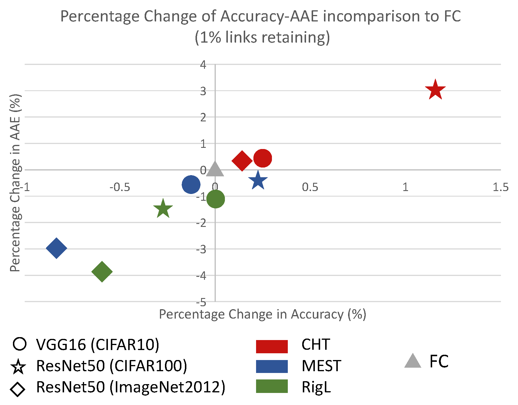
In Figure 3, we present the general performance of CHT, RigL, and MEST relative to the fully connected network (FC). For this comparison, the x-axis and y-axis of the left figure represent the change rate (increase or decrease) in accuracy and area across epochs (AAE, indicating learning speed) compared to the fully connected configuration. The value is computed as

(v - f c) / f c

, where v stands for the measurement of the algorithms and

f c

represents the corresponding fully connected networks’ performance. In this scenario, algorithms positioned further to the upper right of the figure are both more accurate and faster. Table A1 provides the specific performance details corresponding to Figure 3. Observing the figure and the table, CHT (depicted in red) consistently surpasses the other dynamic sparse training methods and even the fully connected network in performance and also exhibits the fastest learning speed. Noteworthily, our method consistently retains only 1% of the links throughout the training.

Sparsity.

Additionally, we delved into a sensitivity analysis of sparsity range from 0.999 to 0.9, depicted in Figure A1C, revealing astonishing results. CHT exhibits good performance even at an ultra-sparse level of 0.999, whereas other dynamic sparse training methods lag behind. This strongly suggests that under the guidance of topological link prediction, dynamic sparse training can rapidly and accurately identify the optimal subnetworks, thereby improving training efficiency with minimal information.

Running time analysis.

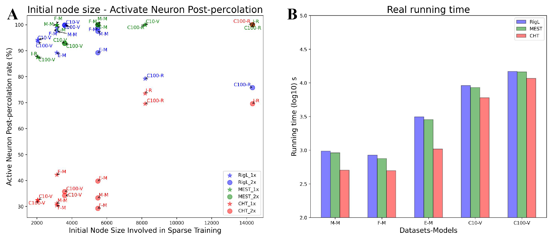
We evaluate the running times of CHT in comparison to other dynamic sparse training methods from two aspects. Firstly, we consider the area across the epochs (AAE), which reflects the learning pace of the algorithms. As emphasized in Table A1, our method consistently surpasses other dynamic sparse training algorithms in learning speed, even outpacing the dense configuration. Secondly, we assess from the standpoint of actual running time. The acceleration benefits are derived from quicker convergence and the early-stop mechanism integrated into topological evolution. Notably, the time complexity for the link regrowth process is

O (N^{4} \times d e n s i t y)

. At very low densities, this complexity approximates

(N^{3})

. Through practical testing on a 1024-1024 network with a density of 1%, the link prediction duration is roughly 1-2 seconds. Although the runtime for the link predictor is slower than the others, we utilize an early-stop approach that truncates topological adjustments within a few epochs. As presented in Figure 4B, which exhibits the actual running times of various algorithms from initiation to convergence, CHT consistently faster than the others. Given CHT’s oracle-like capacity to intuitively suggest the placement of new links that boosting gradient learning, it greatly abbreviates the convergence period for dynamic sparse training.

Adaptive Percolation.

As depicted in Figure 4A, CHT adeptly percolates the network to preserve approximately 30-40% of the initial node size for relatively simpler tasks such as MNIST when applied with MLPs. In contrast, for more complicated tasks like ImageNet on ResNet50, the ANP remains high. This behavior underscores that CHT isn’t just a myopic, greedy algorithm. It seems that intelligently adjusts the number of active neurons based on the complexity of the task at hand, ensuring no compromise on performance even in ultra-sparse scenarios. In contrast, other sparse training methods like RigL do show a lower ANP rate on ImageNet when using ResNet50. However, this reduction is accompanied by a performance drop, possibly because such methods lack task awareness.

This adaptive percolation ability of CHT to provide a minimalistic network modelling that preserves performance with a smaller architecture, is a typical solution in line with the Occam’s razor also named in science as the principle of parsimony, which is the problem-solving principle advocating to search for explanations constructed with the smallest possible set of elements Gauch Jr et al. (2003). On this basis, we can claim that CHT represents the first example of an algorithm for “parsimony ultra-sparse training”. We stress that the parsimony is obtained as an epiphenomenon of the epitopological learning, indeed neither random nor gradient link regrowth is able to trigger the adaptive percolation of ESML or CHT.

5. Conclusion

In this paper, we investigate the design of ultra-sparse (1% links) topology for deep learning in comparison to fully connected, introducing a novel approach termed Epitopological Sparse Meta-deep Learning (ESML), which leverages insights from network science and brain-inspired learning to evolve deep artificial neural network topologies in dynamic ultra-sparse (1% links) training. Furthermore, we present the Cannistraci-Hebb Training (CHT) process, comprising four essential components to augment ESML’s performance. The performance and network analysis indicate that ESML can convert the initial random network into a complex, structured topology, which is more conducive to training and potentially represents a valid lottery-ticket network. Further empirical findings demonstrate that anchored by the 4-step methodology, CHT not only learns more rapidly and accurately but also adaptively percolates the network size based on task complexity. This performance surpasses other dynamic sparse training methods and even outperforms the fully connected network, maintaining only 1% of its links during training. This achievement marks a significant milestone in the field of deep learning. Discussion of Limitations and future challenges is provided in Appendix C.

Appendix A Dynamic sparse training

Let’s first define how the network will learn through gradients with the sparse mask created by dynamic sparse training. Consider

θ \in R^{N}

as the weights matrix of the entire network,

M \in {0, 1}^{N}

is the adjacency matrix of the current existing links inside the model. The general optimization function of can be formulated as:

min_{θ} {L (θ ⊙ M; D) s . t . | | M | |}_{0} \leq k,

(A1)

where the

L (\cdot)

is the loss function and

D

is the training dataset. k is the remaining weights in the entire number N of weights regarding the preset sparsity S,

k = N * (1 - S)

. The main difference between dynamic sparse training and static sparse training is whether it allows the mask M to change dynamically. A standard dynamic sparse training method Evci et al. (2020); Mocanu et al. (2018); Yuan et al. (2021), as illustrated in Figure A3A, begins with a sparse initialized network and undergoes the prune-and-grow regime with multiple iterations after each update interval of weights. In one update iteration, the gradient of the weights can be formulated as:

\frac{\partial L}{\partial θ_{i}} = \frac{\partial L}{\partial (θ_{i} ⊙ M_{i})} M_{i},

(A2)

i indicates the layer index of the model. The main differences between the current standard dynamic sparse training methods are how to remove links and how to regrow new links. SET Mocanu et al. (2018), as the first dynamic sparse training method, removes links with weight magnitude and regrows new links randomly. Different from the removal process of SET, MEST Yuan et al. (2021) also regrows new links randomly while removing weights with the combination of weight magnitude and gradient magnitude of the existing links. RigL Evci et al. (2020) utilizes the gradient magnitude of the missing links to regrow the new links. Some other innovations in dynamic sparse training are adding some tricks or making it more hardware-friendly. Zhang et al. (2023b) introduces a method called Bi-Mask that accelerates the backpropagation process of sparse training with N:M constraint Mishra et al. (2021). SpFDE Yuan et al. (2022) introduces layer freezing and data sieving strategy to further accelerate the training speed of DST. We let you notice that Mixture-of-Experts (MoEs) Riquelme et al. (2021) is also a type of DST method that is widely used in training large language models since the experts are always sparse during training.

However, most methods for training sparse neural networks are not actually sparse during training. For example, RigL Evci et al. (2020) needs to collect gradients for missing connections to regrow new ones. OptG Zhang et al. (2022) trains an extra weight mask to learn the network topology. Only, methods like SET and MEST that randomly regrow connections actually use just the sparse model during training. However, they don’t work as well as methods that use gradient information. So in this paper, we introduce an efficient, gradient-free, and brain-inspired method from network science called epitopological learning to evolve the sparse network topology.

Appendix B Sparse Weight Initialization

Our derivation mainly follows kaimingHe et al. (2015). Similar to SNIPLee et al. (2019) we introduce auxiliary indicator variables

C \in {0, 1}^{m \times n}

. Then For a densely-connected layer, we have:

y_{l} = C_{l} ⊙ W_{l} x_{l} + b_{l},

(A3)

where ⊙ denotes the Hadamard product,

W^{m \times n}

is the weight matrix,

x^{n \times 1}

is the input vector,

b^{m \times 1}

is a vector of biases and

y^{m \times 1}

is the output vector. We use l to index a layer.

Then for i-th element of the pre-activation layer

y_{l}

, by ignoring the influence of bias, we can get its variance:

V a r [y_{l}^{i}] = V a r [\sum_{j = 1}^{n} c_{l}^{i j} w_{l}^{i j} x_{l}^{j}] .

(A4)

As we initialize elements in

C

to be independent and identically distributed random variables, also same for elements in

W

. We also assume elements in

x

are mutually independent and share the same distribution.

C

W

and

x

are independent of each other. Variance of y will be:

V a r [y_{l}^{i}] = n V a r [c_{l}^{i j} w_{l}^{i j} x_{l}^{j}] = n ((V a r [c] + μ_{c}^{2}) (V a r [w] + μ_{w}^{2}) (V a r [x] + μ_{x}^{2}) - μ_{c}^{2} μ_{w}^{2} μ_{x}^{2}),

(A5)

where

μ

is mean. We assume c follows Bernoulli distribution, then the probability mass function is:

f (c) = \{\begin{matrix} S & c = 0 \\ 1 - S & c = 1 \end{matrix},

(A6)

where S denotes the sparsity. We could infer that

V a r [c] = S (1 - S)

and

μ_{c}^{2} = {(1 - S)}^{2}

. Same as previous work He et al. (2015), we define w follow zero-mean Gaussian distribution, therefore

μ_{c}^{2} μ_{w}^{2} μ_{x}^{2} = 0

. And when activation layer is ReLU,

V a r [x_{l}^{i}] + μ_{x_{l}^{i}}^{2} = \frac{1}{2} V a r [y_{l - 1}^{i}]

. Then equation A5 could be changed to:

V a r [y_{l}^{i}] = n (V a r [c] + μ_{c}^{2}) (V a r [w] + μ_{w}^{2}) (V a r [x] + μ_{x}^{2}) = \frac{1}{2} n (1 - S) V a r [w] V a r [y_{l - 1}^{i}],

(A7)

We expect the variance of signal to remain the same across layers

V a r [y_{l}^{i}] = V a r [y_{l - 1}^{i}]

, then:

V a r [w] = \frac{2}{n (1 - S)},

(A8)

We denote

i n d i m

as n, which represents the dimension of the input layer of each sandwich layer. The constant

g a i n

varies depending on the activation function used. For example, when using ReLU, we set

g a i n

\sqrt{2}

. The resulting values of w are sampled from a normal distribution, resulting in the following expression:

S W I (w) \sim N (0, σ^{2}), σ = \sqrt{V a r [w]} = \frac{g a i n}{\sqrt{(1 - S) * i n d i m}},

(A9)

Appendix C Limitations and future challenges

A limitation of not only our proposed method CHT, but of all current sparse training methods, is the current difficulty to deploy such unstructured sparse training methods efficiently in hardware like GPUs or specialized AI accelerators. Some studies Hubara et al. (2021); Zhang et al. (2023b) attempt to integrate semi-structured sparsity patterns to speed up the network, but this often comes at the cost of reduced performance. Most hardware is optimized for dense matrix multiplications, while sparse networks require more dedicated data access patterns. But this limitation could represent also a challenge to address in future studies because the gain in computational speed could be relevant considering that the backpropagation and the gradient search would be implemented with respect to an ultra-sparse structure. Another important limitation to address in next studies is to better understand the process of node percolation, and to design new strategies of node removal that allows to set a priory a wished value of node sparsity lower-bound. The future challenges of dynamic sparse training should be in our opinion to identify novel adaptive mechanisms of epitopological parsimony learning that, for different dataset and network architectures, can adaptively learn any aspect of the network structure such as node layers, node size and link sparsity.

Appendix D Link Removal and Network Percolation in ESML

We detailed our link removal methods and how we implement network percolation in this section.

Firstly, in the removal phase, ESML adopts the commonly used DST removal method that prunes links with lower weights magnitude (Figure A3, left side), which are considered less useful for the model’s performance. We also try an alternative removal method, which combines weight and gradient magnitude as adopted by MEST. However, this approach did not yield any performance improvement to us at least in the tested datasets.

After the process of standard DST link removal, ESML checks and corrects the topology for the presence of inactive neurons that either do not have a connection in one layer side or do not have any connections in both layer sides. When information passes through these inactive neurons, the forward and backward processes can get stuck. Moreover, if a neuron becomes inactive, no new links will be assigned to it in that network according to the formula of CH3-L3. Thus, ESML implements the Inactive Neurons Removal (INR) to eliminate those inactive neurons from the topology. In particular, in the case that inactive nodes possesse connections on one layer side, we need to conduct Incomplete Path Adjustment (IPA) to remove those links. Since IPA may produce some extra inactive neurons, we execute INR and IPA for two rounds. We termed the coupled process of INR and IPA as network percolation, because it is reminiscent of the percolation theory in network science, which studies the connectivity behavior of networks when a fraction of the nodes or edges are removed Li et al. (2021). If there are still some inactive neurons, we leave them in the network and clean up them during the next evolution.

Appendix E Results on the other tasks

In the main text, we showcase the results of CHT on larger datasets and models, while here, we detail CHT’s performance on basic datasets and models. From the results in Table A2, CHT surpasses other dynamic sparse training methods in accuracy on MNIST (MLP) and EMNIST (MLP) while achieving similar performance as others on Fashion_MNIST. Furthermore, CHT stably matches the performance of the fully connected ones in all the tasks. It’s noteworthy that CHT consistently exhibits higher AAEs across all tasks, indicating a faster learning pace.

Table A1. Results of CHT comparing to DST methods and fully connected network (FC) on 1× and 2× cases. In this table, we report the accuracy (ACC) and area across the epochs (AAE) of each case. We executed all the DST methods in an extremely sparse scenario (1%). The best performance among the sparse methods is highlighted in bold, and values marked with “*” indicate they surpass those of the fully connected counterparts.

	CIFAR10(Vgg16)		CIFAR100(ResNet50)		ImageNet(ResNet50)
	ACC (%)	AAE	ACC (%)	AAE	ACC (%)	AAE
Original_Network	-	-	79.763	68.259	-	-
FC_1×	91.52±0.04	87.74±0.03	78.297	65.527	75.042	63.273
RigL_1×	91.60±0.10*	86.54±0.14	78.083	64.536	74.540	60.876
MEST_1×	91.65±0.13*	86.24±0.05	78.467*	65.266	74.408	61.418
CHT_1×	91.68±0.15*	86.57±0.08	79.203*	67.512*	75.134*	63.538*
FC_2×	91.75±0.07	87.86±0.02	78.490	65.760	74.911	63.517
RigL_2×	91.75±0.03	87.07±0.09	78.297	64.796	74.778	61.805
MEST_2×	91.63±0.10	87.35±0.04	78.447	64.982	74.756	62.048
CHT_2×	91.98±0.03*	88.29±0.10*	79.253*	67.370*	74.936*	62.998

Table A2. Result of CHT comparing to RigL and Fully connected network on 1× and 2× cases

	MNIST(MLP)		Fashion_MNIST(MLP)		EMNIST(MLP)
	ACC (%)	AAE	ACC (%)	AAE	ACC (%)	AAE
FC_1×	98.69±0.02	96.33±0.16	90.43±0.09	87.40±0.02	85.58±0.06	81.75±0.10
RigL_1×	97.40±0.07	93.69±0.10	88.02±0.11	84.49±0.12	82.96±0.04	78.01±0.06
MEST_1×	97.31±0.05	93.28±0.04	88.13±0.10	84.62±0.05	83.05±0.04	78.14±0.07
CHT_1×	98.05±0.04	95.45±0.05	88.07±0.11	85.20±0.06	83.82±0.04	80.25±0.20
FC_2×	98.73±0.03	96.27±0.13	90.74±0.13	87.58±0.04	85.85±0.05	82.19±0.12
RigL_2×	97.91±0.09	94.25±0.03	88.66±0.07	85.23±0.08	83.44±0.09	79.10±0.25
MEST_2×	97.66±0.03	94.87±0.09	88.33±0.10	85.01±0.07	83.50±0.09	78.31±0.01
CHT_2×	98.34±0.08	95.60±0.05	88.34±0.07	85.53±0.25	85.43±0.10	81.18±0.15

Appendix F Sensitivity test of ESML and CHT

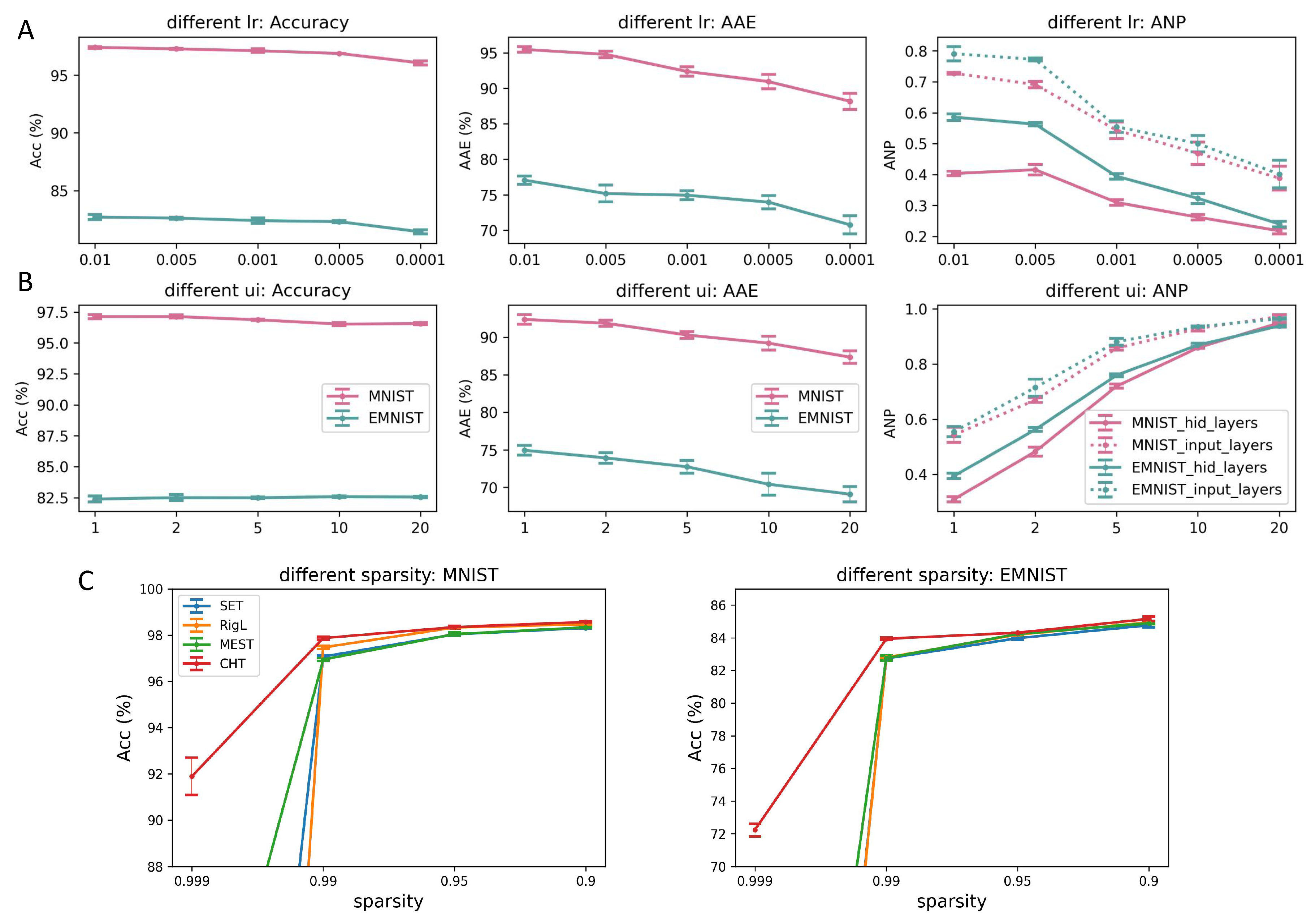
We investigate the influence of hyperparameters which are also significant for the training of ESML and CHT.

Figure A1. Sensitivity test of learning rate, update interval, and sparsity on ESML and CHT. The evaluation measures involve Accuracy, area across the epoch (AAE), and ANP (active neuron post-percolation rate). A shows the impact of learning rate on the MNIST and EMNIST datasets when applied to MLPs. B investigates how varying the update interval of topology affects performance. C illustrates the performance of dynamic sparse training across different sparsity levels on MNIST and EMNIST, with 1x hidden dimension ranging from 0.999 to 0.9. It’s noteworthy that even at 99.9% sparsity, CHT can still learn some information, whereas the other methods cannot. All the experiments are with 3 random seeds.

Learning rate: In particular, learning rate (lr) is a crucial factor that controls the size of the steps taken in each mini-batch during training. In dynamic sparse training, the learning rate is even more dominant. As an example, consider a scenario where weights are assigned to new links with a value of zero. If the learning rate is set to a very small value, these weights may not be able to increase or decrease beyond the positive or negative threshold. Consequently, the weights may get directly pruned in the next round. In Figure A1A, we fix ui=1, sparsity=0.99, and vary lr from [0.01, 0.005, 0.001, 0.0005, 0.0001]. The conclusion drawn from A and B is that a low learning rate could lead to a more percolated network with lower ANP, indicating the effectiveness of ESML in reducing the network size. However, if the learning rate is too small, the network may not be able to learn well due to the slow weight update.

Update interval: The update interval (ui) encounters a similar challenge. If the interval is not appropriately set, it can lead to suboptimal outcomes. The choice of update interval impacts how frequently the network structure is adjusted, and an unsuitable value may hinder the network from effectively adapting to new information. The results show that a larger ui could make the network learn slower and result in a less percolated network.

Sparsity: In our evaluation, we also place significant emphasis on the role of sparsity when assessing the performance of dynamic sparse training methods. Our objective is to delve into the capabilities of these methods in scenarios of extreme sparsity. In Figure A1, we keep ui=1 and lr=0.01 as constants, while we manipulate the sparsity levels within the range of [0.999, 0.99, 0.95, 0.9]. In this setup, we present a comparative analysis of CHT against SET, MEST, and RigL. The purpose is to emphasize the differences among these dynamic sparse training methods as they operate under varying levels of sparsity. Analyzing the results on MNIST and EMNIST, we observed a remarkable trend: even in scenarios with an extreme sparsity level of 99.9% (density=0.1%), where the connectivity is highly sparse, CHT manages to extract and transfer meaningful information. In contrast, both RigL and SET failed to learn anything significant. This disparity in performance can be attributed to the capabilities of link prediction methods in handling sparse information. For CHT, its ability to utilize topology for predicting new connections becomes especially advantageous in situations of extreme sparsity. On the other hand, SET and MEST, which randomly regenerate new connections, face a vast search space, making it exceedingly challenging to identify the correct subnetwork. Meanwhile, RigL struggles in such scenarios due to the limited availability of credit assignment paths (CAPs) in the extremely sparse connectivity, rendering gradient information less useful.

Appendix G Ablation test of each component in CHT

We evaluate each component introduced (CSTI, SWI, and early stop) in CHT in Figure A2 using an example of MNIST on the MLP structure. The first three plots compare CSTI vs. ER initialization, SWI vs. Kaiming weight initialization, and early stop strategy vs. no early stop strategy while keeping the other components fixed.

Correlated Sparse Topology Initialization network properties.

We first report the initialization structure in Figure A4.C which is a Correlated Sparse Topological Initialization (CSTI) example with 2× version of hidden dimension on the MNIST dataset, we construct the heatmap of the input layer degrees and node distribution density curve. It can be clearly observed that with CSTI, the links are assigned to nodes mostly associated to input pixels in the center of figures in MNIST dataset, and indeed the area at the center of the figures is more informative. We also report the CSTI-formed network has an initialized power law exponent

γ

=5.4 which indicates a topology with more hub nodes than in a random network with

γ

=10.

Correlated sparse topological initialization (CSTI):

We demonstrate that with structured topology initialization, ESML can achieve faster learning speed compared to ER initialization. This can be explained by the theory that link predictors are most effective when the network has already formed certain structural features.

Figure A2. Ablation test of each component in CHT on the MLP architecture for MNIST dataset with 1× hidden dimension. The first three figures demonstrate the efficiency of different strategies while keeping the other components fixed and only varying the one being compared. The last figure illustrates the overlap rate of the new links and removed links, providing insight into the necessity of utilizing early stop of the evolutionary process.

Sparse Weight Initialization (SWI):

We assess SWI against the commonly used weight initialization method in dynamic sparse training, Kaiming. The results indicate that SWI facilitates faster training from the initial phases.

Early stop:

The third panel presents evidence that early stop can prevent the over-evolution of the network topology. Once the network structure becomes stable, running ESML is unnecessary, and it is more optimal to conduct early stop and focus on refining the weights to achieve convergence. As an example, at the 12th epoch, the overlap rate (the overlap between removed links and new links) exceeds 90%, which can be seen as a topological stability threshold, indicating that the network should no longer evolve. Based on this observation, we implement an early stop for the evolutionary process. With early stop, we not only achieve performance improvements but also accelerate training speed since there’s no need for further topological exploration.

Appendix H Extra experiments setup

Appendix H.1. Hidden dimension

It’s important to highlight that the hidden dimension settings differ between the evaluations of ESML and CHT in this article. When assessing ESML and comparing it with SET, we adopt the same network structure as outlined in SET (ref), where the hidden dimension is set to 1000 to ensure a fair comparison with SET. For the CHT evaluation, because of the Correlated Sparse Topological Initialization, we utilize two distinct hidden dimension settings: ’1×’, which corresponds to the same size as the input dimension, and ’2×’, which is double the size of the input dimension. All the algorithms are testes considering these two dimensions.

Appendix H.2. Baseline methods

To highlight the potential of link prediction in guiding the formation of new links, in this article, we compare ESML with SET Mocanu et al. (2018) which serves as a foundational method in dynamic sparse training that relies on the random regrowth of new links. To highlight the advantages of CHT, we compare it with two state-of-the-art dynamic sparse training algorithms: RigL Evci et al. (2020) and MEST Yuan et al. (2021). Both of these algorithms follow the prune-and-regrow approach. RigL prunes links by weight magnitude and regrows them based on the gradient magnitude of missing links. Additionally, it features an adaptive

ζ

strategy that gradually reduces the proportion of links pruned and regrown over the training epochs. Conversely, MEST employs a combination of weight and gradient magnitudes of the existing links for link removal and subsequently regrows new links at random. Notably, MEST’s “EM&S" tactic, which enables training from a denser network to a sparse one, is also implemented in this article.

Appendix H.3. Sparsity

In this article, we maintain a sparsity level of 99% (equivalent to 1% density) for all evaluations, except for the sparsity sensitivity test. The sparsity pattern adopted in this study is unstructured. This is because both pattern-based and block-based patterns impose constraints on the network’s topology, potentially detrimentally affecting model performance. Nonetheless, even with unstructured sparsity, CHT facilitates a quicker training acceleration due to its enhanced learning speed and rapid convergence.

Appendix I Area Across the Epochs

The Area Across the Epochs (AAE) is computed as the cumulative sum of the performance indicator of an algorithm till a certain epoch is divided by the number of epochs. Therefore, AAE is the average performance that an algorithm displays till a certain epoch during training, it is bounded [0,1] and it is an indicator of the learning speed of an algorithm. This means that algorithms whose training curves grow faster have larger AAE and can be considered: "faster learners". For instance, considering the same algorithm and fixing the same number of epochs for each trial, AAE can be used to measure and compare the impact that the tuning of a hyperparameter has on learning speed and to quantify the extent to which this hyperparameter governs learning speed.

A A E (A) = \frac{\int m d m}{E - 1},

(A10)

Where A denotes the algorithms that need to be evaluated, E is the number of epochs. m denotes the accuracy at each epoch.

Pay attention, when we come to comparing different algorithms, there are two important remarks about the way to apply AAE for a fair comparison of learning speed.

First, AAE should be applied considering for all different algorithms the same number of epochs and the same hyperparameter settings that can influence learning speed. If an algorithm stops at a number of epochs that is smaller than others then all the algorithms’ AAEs will be computed till this smallest epochs value, to make sure that the algorithms are fairly evaluated considering the same interval of epochs. If two algorithms are run using different update intervals of epochs during training, then the comparison is not fair and both algorithms should be run using the same update intervals, and this is valid for any setting that can influence the learning speed. All learning speed settings should be fairly fixed to the same value across methods to ensure that the learning speed difference between algorithms is intrinsic to the sparse training mechanisms and it is not biased by confounding factors.

Second, AAE can be only used to compare the learning speed of algorithms inside the same computational experiment and not across different datasets and network architectures, because different datasets or network architectures can generate different learning speeds. However, if the mission of the comparison is to investigate the different learning speeds of the same algorithm with the same hyperparameters settings and network structure, but using different datasets, then using AAE is still valid and can help to determine how the same algorithm might react differently in learning speed because of some variations to the data. An interesting test to try is for instance to investigate the impact of different increasing noise levels on the same type of data considering the same algorithm and setting. This would help to reply to the question of how the noise impacts the learning speed of an algorithm.

Figure A3. Illustration of the standard DST progress and ESML. ESML incorporates two additional steps for network evolution, namely network percolation and EL(link prediction). Network percolation involves Inactive Neurons Removal (INR) and the Incomplete Path Adjustment (IPA). In the epitopological learning (EL) part, which is based on link prediction, after dividing the entire network into several sandwich layers, the chosen link predictor (CH3-L3) separately calculates the link prediction score for each non-existing link and then regrows links with top-k scores in equal number to those that were removed.

Figure A4. Main innovations introduced in CHT. A shows an example of how to construct the CSTI on the MNIST dataset, which involves four steps: vectorization, feature correlation, connectivity selection, and assembling topological hubbed network blocks. B presents a real network example of how SWI assigns weights to the sparse network. C displays the input layer degree distribution along with the associated heatmap of 2× case on the MNIST figure template and the node degree distribution. We explain the details of the procedure involved in this figure in Section 3.2.

Figure A5. An explanatory example of topological link prediction performed using CH theory on bipartite networks. The two yellow nodes are the seed nodes whose non-observed interaction should be scored with a likelihood. The green nodes represent the common neighbors (CNs) of the seed nodes in the bipartite network. The red links denote the interactions between CNs, which are referred to as internal local community links (iLCL). The blue links represent the interaction between CNs and external nodes of the community that are not shown in this example which are termed as external local community links (eLCL).

Appendix J Subranking strategy of CH3-L3

Here we describe the sub-ranking strategy adopted by CH3-L3Muscoloni et al. (2020) to internally rank all the node pairs that have the same CH score. Although we didn’t apply this strategy in the current article due to the ultra-sparse scenario, it can be useful for lower-sparsity DST applications in the future. The sub-ranking strategy aims to provide a more precise ranking for links with identical link prediction scores, particularly those that are tied-ranked and located just above the regrown threshold links.

To implement the sub-ranking strategy, the following algorithmic steps are followed:

Assign a weight to each link $(i, j)$ in the network, denoted as $w_{i, j} = \frac{1}{1 + C H_{i, j}}$ .
Compute the shortest paths (SP) between all pairs of nodes in the weighted network.
For each node pair $(i, j)$ , compute the Spearman’s rank correlation ( $S P c o r r$ ) between the vectors of all shortest paths from node i and node j.
Generate a final ranking where node pairs are initially ranked based on the CH score ( $C H_{i, j}$ ), and ties are sub-ranked based on the $S P c o r r_{i, j}$ value. If there are still tied scores, random selection is used to rank the node pairs.

While the

S P c o r r

can be replaced with any other link predictor, we adopted this strategy because it aligns with the neurobiological principles underlying the CH modelMuscoloni et al. (2020). According to the interpretation of Peters’ rule, the probability of two neurons being connected is influenced by the spatial proximity of their respective axonal and dendritic arborsRees et al. (2017). In other words, connectivity depends on the geometric proximity of neurons. This neurobiological concept is consistent with the

S P c o r r

score and fits within the framework of CH modeling, as a high correlation suggests that two nodes have similar shortest paths to other nodes in the network, indicating spatial proximity due to their close geometric positioning.

Table A3. Active neuron post-percolation rate corresponding to the results in Table A3

	MNIST	Fashion_MNIST	EMNIST	CIFAR10	CIFAR100(VGG16)	CIFAR100(ResNet50)	ImageNet(ResNet50)
CHT_1X	31.15%	30.45%	42.22%	32.52%	32.32%	99.98%	73.54%
RigL_1X	97.45%	98.69%	89.19%	94.14%	93.50%	79.22%	36.16%
CHT_2X	33.27%	29.25%	39.78%	34.24%	35.71%	100%	69.57%
RigL_2X	100%	100%	99.82%	99.83%	99.80%	75.74%	29.67%

Appendix K Credit Assigned Path

The epitopological learning implemented via CH3-L3 link prediction produces a topology that encourages new inter-layer links between pair of non-interacting nodes that are topologically close to each other because they share many externally isolated (minimum number of external links in respect to the local community) common neighbors on paths of length 3 (see Figure 2). This means that during epitopological-based dynamic sparse training, the new predicted inter-layer interactions will connect with continuous path nodes with increasing higher degrees across layers, creating a meta-deep structure inside each layer that connects across the layers and that is composed of the nodes that are at the center of the hyperbolic disk because they have a higher degree and therefore they are more central in the hyperbolic geometry. Hence, epitopological sparse meta-deep learning percolates the network triggering a hyperbolic geometry with community and hierarchical depth which is fundamental to increase the number of credit assigned paths (CAP, which is the chain of the transformation from input to output) in the final trained structure. The total number of CAPs in ESML network is 9,095,753 which is much larger (around x10) than the CAPs of SET-random which is 782,032. Even more interestingly, we introduce a new measure for evaluation of sparse network topology arrangement that is the ratio of CAPs that pass by the hub nodes in intermediate layers. In ESML (Revised as ESML) network of Figure 2A, the hubs are the 80 nodes at the center of hyperbolic disk in layer 2 and 3) and the hub-CAPs ratio is 3551460/9095753=0.39, whereas when taking the top 80 nodes with higher degree in the layer 2 and 3 of SET-random network of Figure 2A, the hub-CAPs ratio passing by them is 5596/782032=0.007. This explains how crucial epitopological learning via CH3-L3 link prediction to trigger a layer hierarchical community organized hyperbolic structure at the center of which emerges a cohort of hubs that create a frame that connects across the layers of the network, forming a scale-free topology with power-law distribution

γ

=2.32. The meta-deep structure of these hubs across the layers, which is associated with the hierarchy (because nodes are in the center of the hyperbolic representation) in hyperbolic geometry and to the power-law distribution triggers an ultra-small-world network with higher navigability Cannistraci & Muscoloni (2022).

Appendix L Hyperparameter setting and implementation details

To better increase the reproducibility of this paper, we write here the hyperparameter setting of each section.

Appendix L.1. Hyperparameter setting

For the overall hyperparameter setting, we set a default sparsity=0.99 (except for the sensitivity test), the fraction of removed links zeta=0.3, weight decay=1e-05, batch size=32, and momentum =0.9 for all the MLP and VGG16 tasks. For the learning rate, we use a fixed rate for all tasks except ResNet50. To highlight the distinction between ESML and SET, we set a lower learning rate of 0.0001 in Section 4.1. In Section 4.2, the default learning rate is 0.01 for both MLP and VGG16. For ResNet50, we employ a learning rate warm-up strategy, details of which are provided below.

VGG16 on CIFAR10 and CIFAR100: The model is started by applying image augmentation, which includes random cropping and horizontal flipping. Following augmentation, we normalize each pixel using a standard normalization process. After normalization, the processed samples are passed through several convolutional blocks, each consisting of two or more convolutional layers (3×3 kernel size), followed by a subsequent max-pooling layer (2x2). Subsequently, the features are flattened into a shape of batchsize×512 and proceed to the fully connected layers. We process dynamic sparse training only on these fully connected layers on CNNs. The hidden dimensions of these layers are detailed in the main text; Specifically, for ESML results, we employ a hidden dimension of 1000, while for CHT, we use either 1× or 2× of input dimension after flattened.

ResNet50 on CIFAR100 and ImageNet2012: First, we apply the same image augmentation techniques as CIFAR10 and CIFAR100, including random cropping, horizontal flipping, and standard normalization. Subsequently, these processed images serve as input for ResNet50. The primary layers of ResNet50 are as follows: a 7×7 convolutional layer with 64 filters and a stride of 2, followed by batch normalization and ReLU activation; a 3x3 max-pooling layer with a stride of 2; four residual blocks, each consisting of several bottleneck layers, followed by batch normalization and ReLU activation; a global average pooling layer that reduces the spatial dimensions to 1x1; fully connected layers with an output dimension of 1000. To enhance the evaluation of our approach in the fully connected (FC) layers, we increased the number of fully connected layers from 1 to 4. The hidden dimension was set to either 1× or 2× the input dimension. We trained the network for 90 epochs, employing a learning rate schedule for warm-up. Specifically, the learning rate was multiplied by a factor of 0.1 at epochs 31 and 61, starting with an initial value of 0.1.

The detailed hyperparameter settings of this experiment in Table A1 are as follows: initial learning rate of 0.1, weight decay of 1e-4, momentum of 0.9, a training batch size of 256, a test batch size of 200, sparsity set at 0.99 with no dropout.

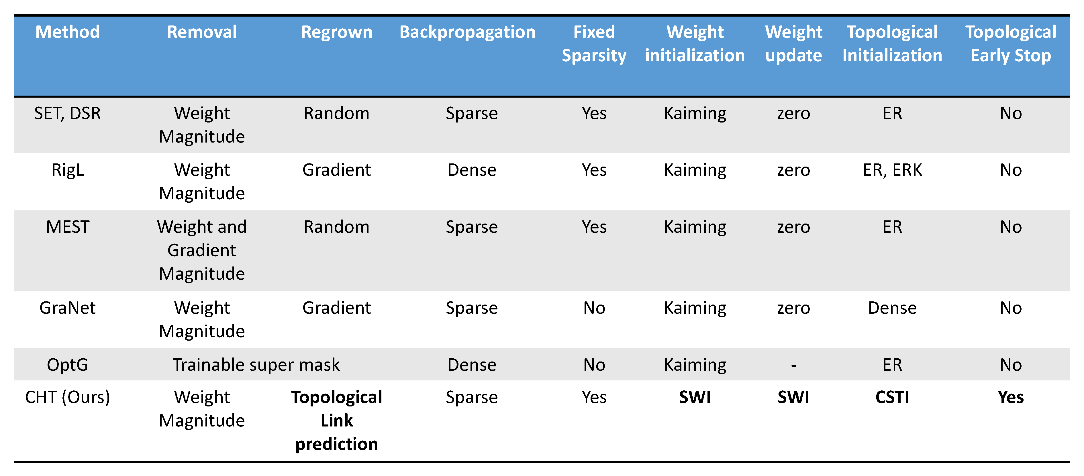
Figure A6. Comparing various components of different pruning and sparse training algorithms. The innovations in this article are highlighted in bold.

Appendix L.2. Algorithm tables of ESML and CHT

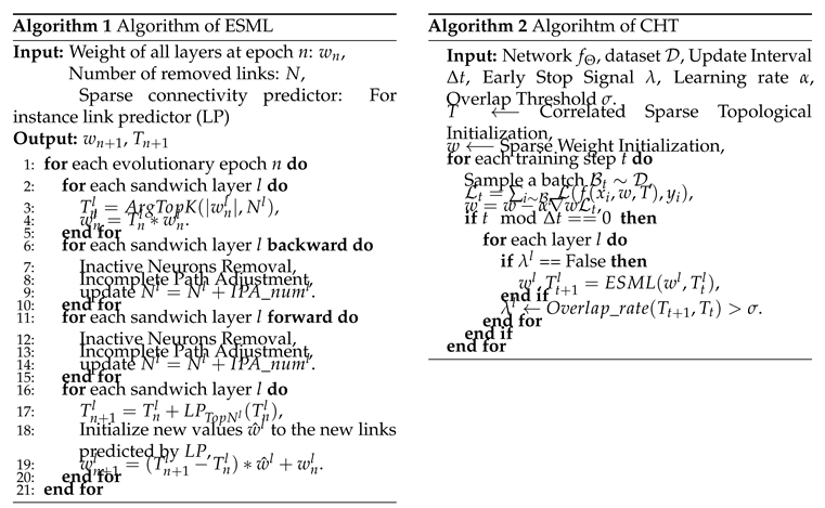
Please refer the Algorithm 1 and Algorithm 2.

Appendix M Annotation in Figure

Because of the page limitation, we report the annotation meaning here. For datasets: “M”, “F”, and “E” stand for MNIST, Fashion_MNIST, and EMNIST, respectively; “C10” and “C100” denote “CIFAR10” and “CIFAR100”; while “I” signifies ImageNet2012. Regarding the models, “M”, “V”, and “R” correspond to MLP, VGG16, and ResNet50, respectively.

References

Muscoloni Alessandro and Cannistraci Carlo Vittorio. Leveraging the nonuniform pso network model as a benchmark for performance evaluation in community detection and link prediction. New Journal of Physics, 20(6):063022, 2018.
Alberto Cacciola, Alessandro Muscoloni, Vaibhav Narula, Alessandro Calamuneri, Salvatore Nigro, Emeran A Mayer, Jennifer S Labus, Giuseppe Anastasi, Aldo Quattrone, Angelo Quartarone, et al. Coalescent embedding in the hyperbolic space unsupervisedly discloses the hidden geometry of the brain. arXiv preprint arXiv:1705.04192, 2017.
Carlo Vittorio Cannistraci. Modelling self-organization in complex networks via a brain-inspired network automata theory improves link reliability in protein interactomes. Sci Rep, 8(1):2045–2322, 10 2018.
Carlo Vittorio Cannistraci and Alessandro Muscoloni. Geometrical congruence, greedy navigability and myopic transfer in complex networks and brain connectomes. Nature Communications, 13(1):7308, 2022.
Carlo Vittorio Cannistraci, Gregorio Alanis-Lobato, and Timothy Ravasi. From link-prediction in brain connectomes and protein interactomes to the local-community-paradigm in complex networks. Scientific reports, 3(1):1613, 2013.
Gregory Cohen, Saeed Afshar, Jonathan Tapson, and Andre Van Schaik. Emnist: Extending mnist to handwritten letters. In 2017 international joint conference on neural networks (IJCNN), pp. 2921–2926. IEEE, 2017.
Simone Daminelli, Josephine Maria Thomas, Claudio Durán, and Carlo Vittorio Cannistraci. Common neighbours and the local-community-paradigm for topological link prediction in bipartite networks. New Journal of Physics, 17(11):113037, nov 2015. URL. [CrossRef]
Claudio Durán, Simone Daminelli, Josephine M Thomas, V Joachim Haupt, Michael Schroeder, and Carlo Vittorio Cannistraci. Pioneering topological methods for network-based drug–target prediction by exploiting a brain-network self-organization theory. Briefings in Bioinformatics, 19(6):1183–1202, 04 2017. URL. [CrossRef]
Utku Evci, Trevor Gale, Jacob Menick, Pablo Samuel Castro, and Erich Elsen. Rigging the lottery: Making all tickets winners. In Proceedings of the 37th International Conference on Machine Learning, ICML 2020, 13-18 July 2020, Virtual Event, volume 119 of Proceedings of Machine Learning Research, pp. 2943–2952. PMLR, 2020. URL http://proceedings.mlr.press/v119/evci20a.html.
Elias Frantar and Dan Alistarh. Massive language models can be accurately pruned in one-shot. arXiv preprint arXiv:2301.00774, 2023.
Hugh G Gauch Jr, Hugh G Gauch, and Hugh G Gauch Jr. Scientific method in practice. Cambridge University Press, 2003.
Xavier Glorot and Yoshua Bengio. Understanding the difficulty of training deep feedforward neural networks. In Yee Whye Teh and D. Mike Titterington (eds.), Proceedings of the Thirteenth International Conference on Artificial Intelligence and Statistics, AISTATS 2010, Chia Laguna Resort, Sardinia, Italy, May 13-15, 2010, volume 9 of JMLR Proceedings, pp. 249–256. JMLR.org, 2010. URL http://proceedings.mlr.press/v9/glorot10a.html.
Babak Hassibi, David G Stork, and Gregory J Wolff. Optimal brain surgeon and general network pruning. In IEEE international conference on neural networks, pp. 293–299. IEEE, 1993.
Kaiming He, Xiangyu Zhang, Shaoqing Ren, and Jian Sun. Delving deep into rectifiers: Surpassing human-level performance on imagenet classification. In Proceedings of the IEEE international conference on computer vision, pp. 1026–1034, 2015.
Kaiming He, Xiangyu Zhang, Shaoqing Ren, and Jian Sun. Deep residual learning for image recognition. In Proceedings of the IEEE conference on computer vision and pattern recognition, pp. 770–778, 2016.
Donald Hebb. The organization of behavior. emphnew york, 1949.
Itay Hubara, Brian Chmiel, Moshe Island, Ron Banner, Joseph Naor, and Daniel Soudry. Accelerated sparse neural training: A provable and efficient method to find n: m transposable masks. Advances in neural information processing systems, 34:21099–21111, 2021.
Alex Krizhevsky. Learning multiple layers of features from tiny images. pp. 32–33, 2009. URL https://www.cs.toronto.edu/~kriz/learning-features-2009-TR.pdf.
Yann LeCun, John S. Denker, and Sara A. Solla. Optimal brain damage. In David S. Touretzky (ed.), Advances in Neural Information Processing Systems 2, [NIPS Conference, Denver, Colorado, USA, November 27-30, 1989], pp. 598–605. Morgan Kaufmann, 1989. URL http://papers.nips.cc/paper/250-optimal-brain-damage.
Yann LeCun, Léon Bottou, Yoshua Bengio, and Patrick Haffner. Gradient-based learning applied to document recognition. Proc. IEEE, 86(11):2278–2324, 1998. URL. [CrossRef]
Namhoon Lee, Thalaiyasingam Ajanthan, and Philip H. S. Torr. Snip: single-shot network pruning based on connection sensitivity. In 7th International Conference on Learning Representations, ICLR 2019, New Orleans, LA, USA, May 6-9, 2019. OpenReview.net, 2019. URL https://openreview.net/forum?id=B1VZqjAcYX.
Jiajun Li and Ahmed Louri. Adaprune: An accelerator-aware pruning technique for sustainable cnn accelerators. IEEE Transactions on Sustainable Computing, 7(1):47–60, 2021.
Ming Li, Run-Ran Liu, Linyuan Lü, Mao-Bin Hu, Shuqi Xu, and Yi-Cheng Zhang. Percolation on complex networks: Theory and application. Physics Reports, 907:1–68, 2021.
Linyuan Lü, Liming Pan, Tao Zhou, Yi-Cheng Zhang, and H. Eugene Stanley. Toward link predictability of complex networks. Proceedings of the National Academy of Sciences, 112(8):2325–2330, 2015.
Asit Mishra, Jorge Albericio Latorre, Jeff Pool, Darko Stosic, Dusan Stosic, Ganesh Venkatesh, Chong Yu, and Paulius Micikevicius. Accelerating sparse deep neural networks. arXiv preprint arXiv:2104.08378, 2021.
Decebal Constantin Mocanu, Elena Mocanu, Peter Stone, Phuong H Nguyen, Madeleine Gibescu, and Antonio Liotta. Scalable training of artificial neural networks with adaptive sparse connectivity inspired by network science. Nature communications, 9(1):1–12, 2018.
A. Muscoloni, U. Michieli, and C.V. Cannistraci. Adaptive network automata modelling of complex networks. preprints, 2020. URL. [CrossRef]
Alessandro Muscoloni and Carlo Vittorio Cannistraci. A nonuniform popularity-similarity optimization (npso) model to efficiently generate realistic complex networks with communities. New Journal of Physics, 20(5):052002, 2018.
Alessandro Muscoloni and Carlo Vittorio Cannistraci. Angular separability of data clusters or network communities in geometrical space and its relevance to hyperbolic embedding. arXiv preprint arXiv:1907.00025, 2019.
Vaibhav et al Narula. Can local-community-paradigm and epitopological learning enhance our understanding of how local brain connectivity is able to process, learn and memorize chronic pain? Applied network science, 2(1), 2017.
Mark EJ Newman. Clustering and preferential attachment in growing networks. Physical review E, 64(2):025102, 2001.
Christopher L Rees, Keivan Moradi, and Giorgio A Ascoli. Weighing the evidence in peters’ rule: does neuronal morphology predict connectivity? Trends in neurosciences, 40(2):63–71, 2017.
Carlos Riquelme, Joan Puigcerver, Basil Mustafa, Maxim Neumann, Rodolphe Jenatton, André Susano Pinto, Daniel Keysers, and Neil Houlsby. Scaling vision with sparse mixture of experts. Advances in Neural Information Processing Systems, 34:8583–8595, 2021.
Olga Russakovsky, Jia Deng, Hao Su, Jonathan Krause, Sanjeev Satheesh, Sean Ma, Zhiheng Huang, Andrej Karpathy, Aditya Khosla, Michael Bernstein, Alexander C. Berg, and Li Fei-Fei. ImageNet Large Scale Visual Recognition Challenge. International Journal of Computer Vision (IJCV), 115(3):211–252, 2015.
Karen Simonyan and Andrew Zisserman. Very deep convolutional networks for large-scale image recognition. arXiv preprint arXiv:1409.1556, 2014.
Mingjie Sun, Zhuang Liu, Anna Bair, and J Zico Kolter. A simple and effective pruning approach for large language models. arXiv preprint arXiv:2306.11695, 2023.
Han Xiao, Kashif Rasul, and Roland Vollgraf. Fashion-mnist: a novel image dataset for benchmarking machine learning algorithms. arXiv preprint arXiv:1708.07747, 2017.
Mengqiao Xu, Qian Pan, Alessandro Muscoloni, Haoxiang Xia, and Carlo Vittorio Cannistraci. Modular gateway-ness connectivity and structural core organization in maritime network science. Nature Communications, 11(1):2849, 2020.
Geng Yuan, Xiaolong Ma, Wei Niu, Zhengang Li, Zhenglun Kong, Ning Liu, Yifan Gong, Zheng Zhan, Chaoyang He, Qing Jin, et al. Mest: Accurate and fast memory-economic sparse training framework on the edge. Advances in Neural Information Processing Systems, 34:20838–20850, 2021.
Geng Yuan, Yanyu Li, Sheng Li, Zhenglun Kong, Sergey Tulyakov, Xulong Tang, Yanzhi Wang, and Jian Ren. Layer freezing & data sieving: Missing pieces of a generic framework for sparse training. arXiv preprint arXiv:2209.11204, 2022.
Y. Zhang, H. Bai, H. Lin, J. Zhao, L. Hou, and C.V. Cannistraci. An efficient plug-and-play post-training pruning strategy in large language models. preprints, 2023a. URL. [CrossRef]
Yuxin Zhang, Mingbao Lin, Mengzhao Chen, Fei Chao, and Rongrong Ji. Optg: Optimizing gradient-driven criteria in network sparsity. arXiv preprint arXiv:2201.12826, 2022.
Yuxin Zhang, Yiting Luo, Mingbao Lin, Yunshan Zhong, Jingjing Xie, Fei Chao, and Rongrong Ji. Bi-directional masks for efficient n: M sparse training. arXiv preprint arXiv:2302.06058, 2023b.

1	A video that shows the ESML percolation of the network across the epochs for the example of Figure 2A is provided at this link https://shorturl.at/blGY1

Figure 1. The comparison of CH3-L3 (ESML) and random (SET). In the first row, we report the accuracy curves of CH3-L3 (ESML) and random (SET) on 5 datasets and mark the increment at the 250th epoch on the upper right corner of each panel. The second row reports the value of area across the epochs (AAE) which indicates the learning speed of different algorithms corresponding to the upper accuracy plot. Each panel reports the percentage increase.

Figure 2. Network science analysis of the sparse ANNs topology. Various states of the network in A (a 1% density MLP trained on EMNIST) are depicted through both a plain representation and a 2D hyperbolic embedding. This includes the network randomly initialized, the network at its final epoch after Random (SET), and the network at its final epoch after CH3-L3 (ESML) training. The blocks within the network also report two key metrics: the angular separability index (ASI, which signifies the capacity to distinguish communities) and the power law exponent

γ

(reflecting degree distribution). The ESML panel also displays the active neuron post-percolation rate (ANP) trend over the epochs. B shows the results of four network topological measures drawn from the average of five datasets by CH3-L3 (ESML) and random (SET). The shadow area represents the standard error across these five datasets.

γ

Figure 3. Percentage Change in Accuracy-AAE for Dynamic Sparse Training Methods Retaining 1% of Links Compared to a Fully Connected Network (FC). Each scatter indictes the performance of 1× in that dataset. Note that in every task, CHT (red) surpasses the fully connected network in both performance and training speed.

Figure 4. Active Neuron Post-percolation rate and real running time of the dynamic sparse training methods. A shows the incremental or reduction in Active Neuron Post-percolation corresponds to the initial node size. Each point’s annotation represents the case using the format “Dataset-Model” (Please refer to Appendix M). B shows the real running time (log10) of each “Dataset-Model” task. This running time is computed from starting training to model convergence of 1× case.

Disclaimer/Publisher’s Note: The statements, opinions and data contained in all publications are solely those of the individual author(s) and contributor(s) and not of MDPI and/or the editor(s). MDPI and/or the editor(s) disclaim responsibility for any injury to people or property resulting from any ideas, methods, instructions or products referred to in the content.

© 2023 by the authors. Licensee MDPI, Basel, Switzerland. This article is an open access article distributed under the terms and conditions of the Creative Commons Attribution (CC BY) license (http://creativecommons.org/licenses/by/4.0/).

Copyright: This open access article is published under a Creative Commons CC BY 4.0 license, which permit the free download, distribution, and reuse, provided that the author and preprint are cited in any reuse.

MDPI Initiatives

Important Links

Choose an area of interest and we will send you notifications of new preprints at your preferred frequency.

Disclaimer

Ultra-Sparse Network Advantage in Deep Learning via Cannistraci-Hebb Brain-Inspired Training With Hyperbolic Meta-Deep Community-Layered Epitopology

Abstract

1. Introduction

2. Related Work

2.1. Dynamic sparse training

2.2. Epitopological Learning and Cannistraci-Hebb network automata theory for link prediction

3. Epitopological sparse meta-deep learning and Cannistraci-Hebb training

3.1. Epitopological sparse meta-deep learning (ESML)

3.2. Cannistraci-Hebb training

4. Results

4.1. Setup

4.2. Results for ESML and Network analysis of epitopological-based link regrown

4.2.1. ESML prediction performance

4.2.2. Network Analysis

Network percolation.

Hyperbolic hierarchical organization.

Hyperbolic community organization.

The emergency of meta-depth

4.2.2.5. Network measure analysis

4.3. Results of CHT

4.3.0.6. Main Results.

Sparsity.

Running time analysis.

Adaptive Percolation.

5. Conclusion

Appendix A Dynamic sparse training

Appendix B Sparse Weight Initialization

Appendix C Limitations and future challenges

Appendix D Link Removal and Network Percolation in ESML

Appendix E Results on the other tasks

Appendix F Sensitivity test of ESML and CHT

Appendix G Ablation test of each component in CHT

Appendix H Extra experiments setup

Appendix H.1. Hidden dimension

Appendix H.2. Baseline methods

Appendix H.3. Sparsity

Appendix I Area Across the Epochs

Appendix J Subranking strategy of CH3-L3

Appendix K Credit Assigned Path

Appendix L Hyperparameter setting and implementation details

Appendix L.1. Hyperparameter setting

Appendix L.2. Algorithm tables of ESML and CHT

Appendix M Annotation in Figure

References

MDPI Initiatives

Important Links

Subscribe