1. Introduction
As communities adapt to changes in local weather extremes brought on by climate change, accessing the best and latest information available at locally relevant scales is essential. However, climate models typically operate at spatial scales out of step with hydrological, ecological, economic decision-making needs and must be downscaled to higher spatial resolutions. The use of statistical downscaling is widespread for climate model outputs, however there remains a shortage of methods that can downscale precipitation from Atmosphere-Ocean General Circulation Model (AOGCM) simulated precipitation to regional-scale gridded precipitation (Tryhorn et. al. 2011, Chaudhuri et. al., 2017). Precipitation information, especially extremes, is critical for flood modelling and mitigation (Hirabayashi et al. 2013). There is considerable intrinsic complexity in precipitation compared to other climate variables such as temperature or pressure. Precipitation is more dispersed in space and associations at various atmospheric scales (local, meso, synoptic) are more apparent in observed precipitation trends. It is extremely challenging to model such patterns using continuous functions used in conventional statistical downscaling methods, incorporating nonlinearities into downscaling functions is seen as critically important if accurate representations are to be realized (Weichert and Burger 1998). The latest developments in machine learning (ML) approaches such as convolutional neural networks have started to tackle these long-standing problems (Shi et al. 2015). However, commonly used loss functions such as Mean Absolute Error (MAE) and Nash-Sutcliffe Loss (NS) optimize for overall simulation efficiency but neglect precipitation spatial structure; a crucial property if replicating observed local trends is a goal (Plouffe et al. 2015). Narrowly specified loss functions hinder the ability of machine learning models in downscaling, contributing to weak output of regional scale models (Zhang et al. 2006).
In the context of climate change science, severe precipitation can lead to flooding, changes in hydrological morphology, and contribute to water pollution (Carpenter et al., 2018; Eekhout et al., 2018; Raghavendra et al., 2010). In comparison to normal precipitation, extreme precipitation is unpredictable, ambiguously defined, and more fragmented in space, which is difficult to forecast with any certainty (Lee et al., 2017). Downscaling experiments have also found extreme precipitation to be challenging to reproduce at meaningful local scales (Castellano and DeGaetano, 2016). Anticipating changes in extreme precipitation remains an urgent climate information need in many regions of the world.
Global Climate Models (GCMs) have been widely used to obtain climate change data under various scenarios to determine the potential impacts of climate change on hydrological processes in nature (Cho et al., 2016; Li et al., 2017). However, the native resolution of GCMs are too coarse which makes them not suitable for hydrological studies if used directly (Xu, 1999). To mitigate this problem downscaling techniques have evolved where large-scale atmospheric data given by AOGCMs are used along with regional scale observations to generate high-resolution realizations of the variable of interest at over a specified area (Chen et al., 2012). There are two primary types of downscaling methods, statistical and dynamical downscaling (Yhang et al., 2017). Statistical downscaling is more common in climate change impact studies due to its clear design methodology, computational ease and the ability to generate synthetic datasets of any desired length (Hidalgo et al., 2008; Maraun, D., et al. 2010; Trzaska, Sylwia & Schnarr, Emilie. 2014; Widmann et al., 2003).
Popular statistical downscaling techniques include the transfer function method, weather pattern method, and stochastic weather generators (Kioutsioukis et al. 2008; Murphy et al. 2004; Wilby and Harris 2006). Linear regression was used frequently in the past to connect circulation factors with weather variables (Huth, 2002; Zorita and von Storch, 1999). However, these relationships are always complex and non-linear, making it hard to achieve acceptable downscaling results with linear relationships (Ghosh and Mujumdar, 2008). As a result, in recent years machine learning methods have been gaining popularity given their ability to model non-linear relationships between predictor and predictants (Chaudhary et al., 2019; Yi et al., 2018).
Machine learning and data science methods have significantly expanded in various fields in recent years leading to application of tools in new areas and development of new domain-specific variants of existing computational methods. Convolutional neural network (CNN) modelling has become common due to lower computational requirements than the complex dense networks (LeCun et. al. 1998). There are a wide variety of CNN implementations including satellite image change detection (Wang et al. 2019), image segmentation (Ronneberger et. al. 2015), image recognition (Krizhevsky et. al. 2017). The approach used by CNNs for increasing image resolution (Dong et. al. 2014) is an algorithm that is very close in some respects to downscaling of climate model outputs. The central question in these studies is simply, how do we detect and move representative information from one scale down to another scale?
CNNs, which have seen widespread adoption for image processing applications in a variety of fields, cannot recognize the variability present in the results when trained through the general loss functions. This leads to the degradation in performance of CNNs when the training loss function cannot provide significant gradients to the parameters of the network. We believe that the development of appropriate loss functions is integral to application of CNNs (Zhao et al. 2016). Goodfellow et al. (2014) recommended the Generative Adversarial Training (GAN), in which a zero-sum game is played between two networks and in recent years was commonly used in training deep neural networks. This approach provides superior network training and can yield results that appear superficially like the truth and intuitively tackle the issue of gradients.
In this paper we develop a new GAN downscaling approach which can downscale annual maximum rainfall from several AOGCMs to regional-scale gridded annual maximum rainfall at various sites. This has the potential therefore to develop regionally specific downscaling models incorporating local landcover and topography into the downscaling model. The following specific research objectives are tackled by this study;
Develop a methodology to downscale large-scale precipitation, given by several AOGCMs, to regional-scale precipitation at multiple regions of interest by statistical downscaling using Convolution Neural Network and Generative Adversarial Training.
Analyze the effect of input DEM and Land-use/ Land-cover on the simulation output.
Evaluating the efficacy of the novel loss function that incorporates content loss, structural loss and adversarial loss that enhances the estimation of the downscaled precipitation’s global and regional quality.
2. Methods
2.1. Study Area and Datasets
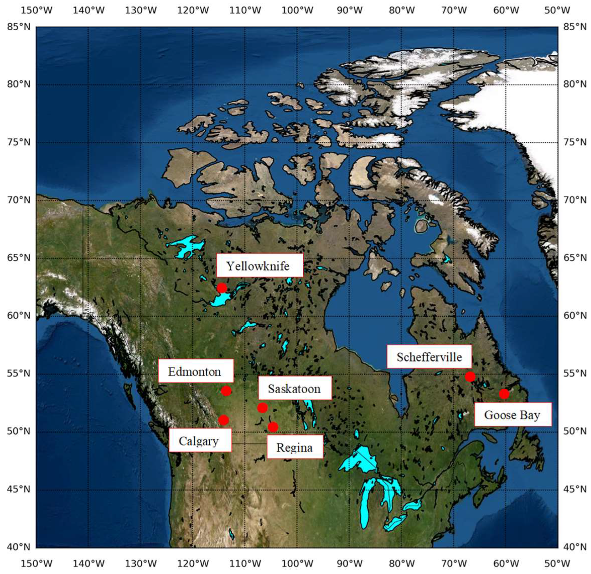
The model is developed for seven cities located in different regions of Canada. The locations of these cities are given in
Figure 1. Individual location plots are shown in Figure S1. The salient features of these regions are summarized in
Table 1.
We used annual maximum daily precipitation as our target variable to establish a downscaling methodology. Annual maximum daily precipitation data from the NRCANMET daily gridded precipitation dataset (Hutchinson et al. 2009) were extracted for the period 1950-2010. Although grid data derived from Canada’s complex observation network density is not ideal validation data, these are the best available data for these regions and should reasonably capture regional trends. Wilby et al. (1999) and Wetterhall et al. (2005) addressed the properties of any predictor in statistical downscaling, (1) it should be simulated by GCMs with high reliability, (2) it can be easily accessed from the archives of GCM outputs, and (3) it has a strong correlation with the surface variables of interest (rainfall in the present case). GCMs simulated rainfall includes atmospheric dynamic information as well as knowledge about the impact of climate change on rainfall through various physical parameterizations. It encouraged us to choose the precipitation simulated by AOGCM as a predictor of the observed (i.e., gridded) precipitation.
Table 1.
Salient geographical and climatic features of the regions of interest.
Table 1.
Salient geographical and climatic features of the regions of interest.
| Name of City |
Area (sq. Km) |
Elevation (m) |
Population |
Temperature Range (°C) |
Average Monthly
Precipitation Range (mm) |
| Schefferville |
39 |
513 |
213 |
−24.5 to 12.2 |
29.7 to 114.6 |
| Goose Bay |
305.69 |
12 |
8109 |
−17.6 to 15.5 |
56.8 to 121.3 |
| Yellowknife |
136.22 |
206 |
19,569 |
−25.6 to 17.0 |
11.3 to 40.8 |
| Edmonton |
767.85 |
645 |
932,546 |
−12.1 to 16.2 |
12.0 to 93.8 |
| Calgary |
825.56 |
1045 |
1,239,220 |
−7.1 to 16.2 |
9.4 to 94.0 |
| Saskatoon |
228.13 |
481.5 |
246,376 |
−15.5 to 18.5 |
8.8 to 65.8 |
| Regina |
179.97 |
577 |
215,106 |
−14.7 to 18.9 |
9.4 to 70.9 |
Figure 1.
The locations of the cities are shown against Canada in red circles.
Figure 1.
The locations of the cities are shown against Canada in red circles.
This research included nine AOGCMs of the CMIP6 database (
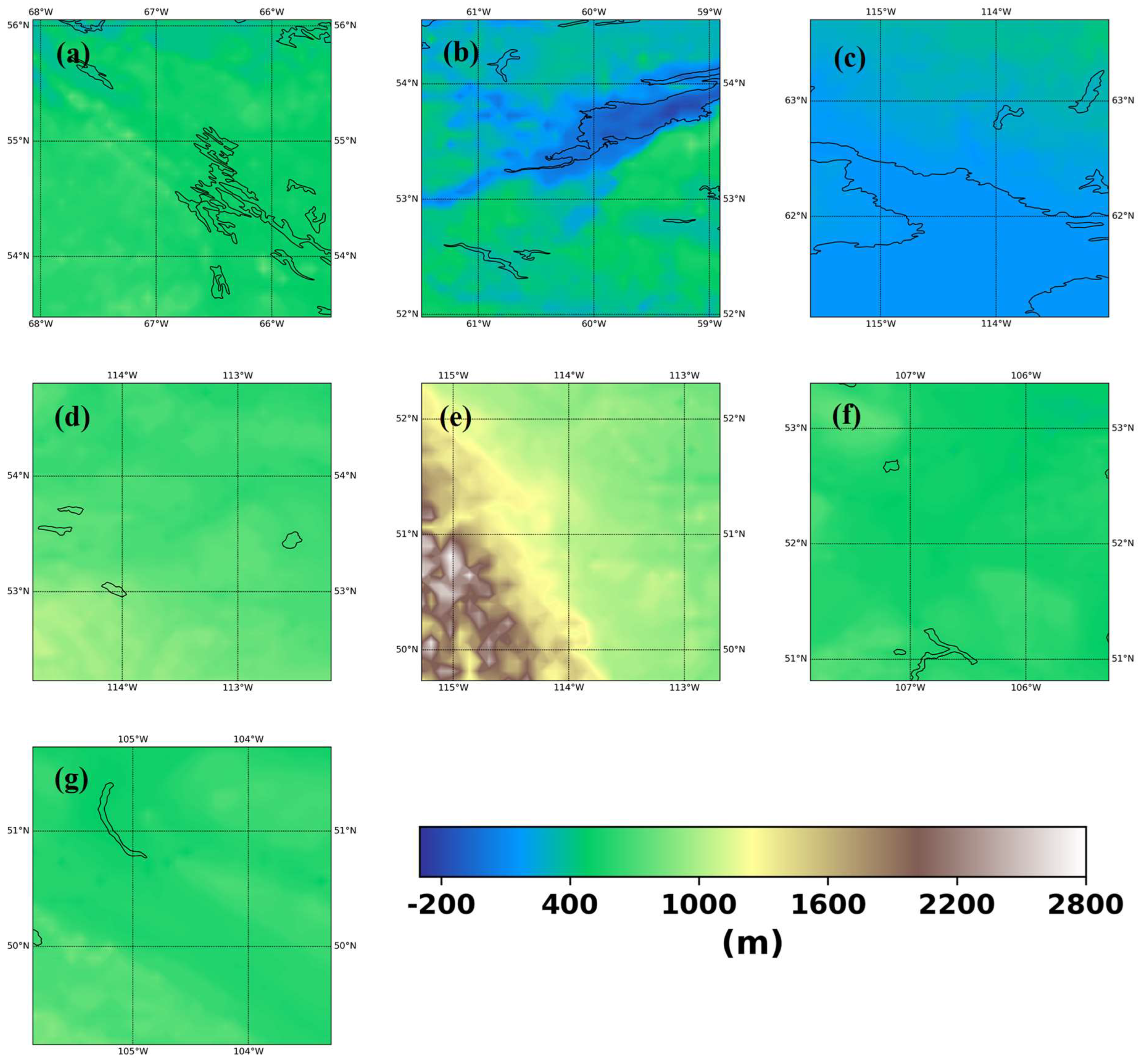
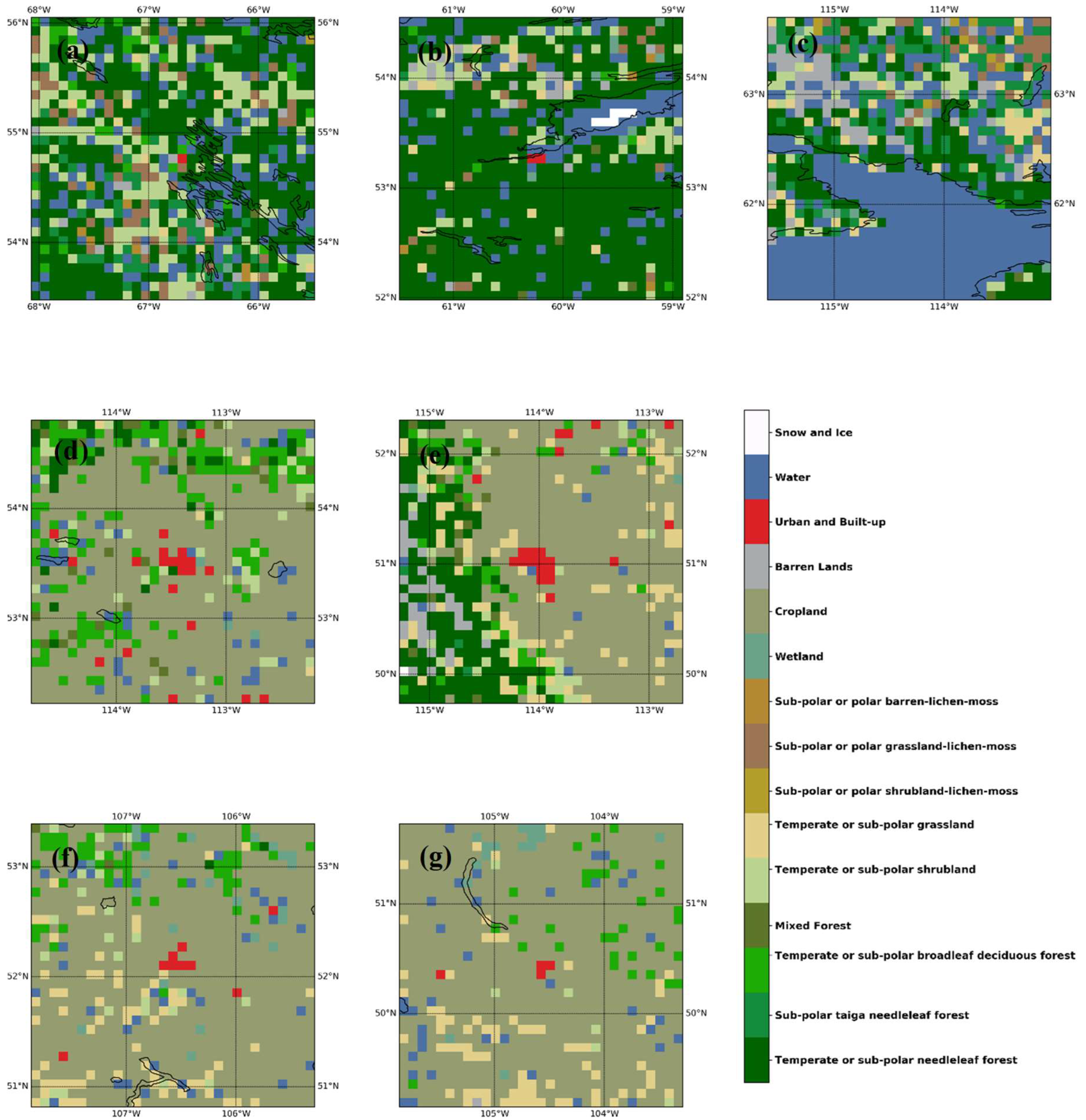
Table 1). Different AOGCMs have different grids and many of them are in Gaussian grids, making it difficult to view them in a single mathematical framework. We have interpolated precipitation from different AOGCMs to 10 km resolution grids specified in output to address this obstacle. Further, we used GEBCO (GEBCO Compilation Group, 2019) land and ocean terrain model as topographic input and 2010 Canada Land cover (Canada Centre for Remote Sensing, 2019) as LULC input to our model. Topography was interpolated to the input grids using a bi-quadratic interpolation function.
Figure 2 shows the topography over 7 regions of interest. The LULC was resampled using dominant categories over the input grid.
Figure 3 shows the dominant LULC grid over the 7 cities where we are building the downscaling model.
Table 2.
Features of different input AOGCMs.
Table 2.
Features of different input AOGCMs.
| AOGCM |
Institution |
Grid Type |
Horizontal Dimension
(Lon × Lat) |
Vertical
Levels |
| BCC ESM |
Beijing Climate Center |
T42 |
128 × 64 |
26 |
| CAN ESM5 |
Canadian Centre for Climate Modelling and Analysis, Environment and Climate Change Canada |
T63 |
128 × 64 |
49 |
| CESM2 |
National Center for Atmospheric Research |
0.9 × 1.25
finite volume grid |
288 × 192 |
70 |
| CNRM CM6.1 |
Centre National de Recherches Meteorologiques |
T127 |
256 × 128 |
91 |
| CNRM ESM2 |
Centre National de Recherches Meteorologiques |
T127 |
256 × 128 |
91 |
| GFDL CM4 |
Geophysical Fluid Dynamics Laboratory |
C96 |
360 × 180 |
33 |
| HAD GEM3 |
Met Office Hadley Centre |
N96 |
192 × 144 |
85 |
| MRI |
Meteorological Research Institute, Tsukuba, Ibaraki 305-0052, Japan |
TL159 |
320 × 160 |
80 |
| UK ESM1 |
Met Office Hadley Centre |
N96 |
192 × 144 |
85 |
Figure 2.
Topography for (a) Schefferville, (b) Goose Bay, (c) Yellowknife, (d) Edmonton, (e) Calgary, (f) Saskatoon, (g) Regina.
Figure 2.
Topography for (a) Schefferville, (b) Goose Bay, (c) Yellowknife, (d) Edmonton, (e) Calgary, (f) Saskatoon, (g) Regina.
Figure 3.
Land-Use/Land-Cover for (a) Schefferville, (b) Goose Bay, (c) Yellowknife, (d) Edmonton, (e) Calgary, (f) Saskatoon, (g) Regina.
Figure 3.
Land-Use/Land-Cover for (a) Schefferville, (b) Goose Bay, (c) Yellowknife, (d) Edmonton, (e) Calgary, (f) Saskatoon, (g) Regina.
2.2. Downscaling Method
We developed a generating network
that can turn extreme precipitation AOGCM coarse resolution (P
GCM) into extreme precipitate (P
obs) fine resolution at the regional level. Increasing resolution, bias correction and regional precipitation feature corrections are the technical challenges of this problem. The number of years for training y = 1, …, n then the θ
G is obtained by minimizing the downscaling total loss function
;
We developed a weighted combination of many components for downscaling total loss. These elements are discussed later in details.
2.2.1. Adversarial Training
As a discriminatory network (Goodfellow et al. 2014), Wasserstein GAN (WGAN) (Arjovsky et. al. 2017) is used in our context. The Earth-Mover (also called Wasserstein-1) distance W(q, p), which is informally defined as a minimum cost to transport mass to convert the distribution q into p (where the cost is mass times transportation distance), was approximated. Formally, the game between the generator
and the discriminator
is a minimax objective. The WGAN loss function is developed using the Kantorovich-Rubinstein [Villani 2008] duality to obtain;
where, D is the set of 1-Lipschitz functions. To satisfy the Lipschitz constraint on the WGAN, Arjovsky et. al. (2017) propose clipping of the weights of the WGAN to ensure that the function lies within a compact space [−c, c]. The set of functions (discriminator under training) satisfying this constraint are subsets of the k-Lipschitz functions for some k which depends on c and the WGAN architecture.
2.2.3. Downscaling Total Loss
In our framework the Total loss is designed as a linear combination of 3-loss components: content loss, structural loss, adversarial loss.
Content Loss
The Nash–Sutcliffe model efficiency coefficient (NSE) is widely used loss estimate which assesses the predictive ability of any hydrology model. We have taken (1-NSE) as content loss.
This loss can take range 0 to . A value of 0 loss means perfect match with the observation. The loss value 1 means that the model is as accurate as the average of the observed values. The loss greater than 1 signifies that the observed mean is a better predictor than the model.
Structural Loss
The overall low error cannot maintain the regional information common to precipitation at high resolution. We implemented a structural loss function to tackle this problem and preserve regional details. The luminance, contrast, and structure of two 2D fields are compared by the Structural Similarity Index (SSIM) (Wang et al. 2003). This matric was compared to preserve the regional precipitation structure on a fine scale. Our loss was described by (1-SSIM)/2 based on structural dissimilarity.
,
, and
are weights of luminance, contrast, and structure components respectively at scale
i. We used α = β = γ = 1. For any given scale the luminance comparison is given by;
The contrast comparison is given by;
and the structure comparison is given by;
where
and
are the mean of observation and generated values respectively,
and
are standard deviation of observation and generated values respectively, and
is the co-variance between observation and generated values.
,
, and
are small constants to stabilize the divisions with weak denominator. We used
,
,
where
,
and
is the dynamic range of the input which we have taken as 100. We used a scale of 3x3 windows to define SSIM.
Adversarial Loss
Adversarial loss is given by the approximate earth moving distance between the observation and generator output. It is given by;
2.2.4. Networks
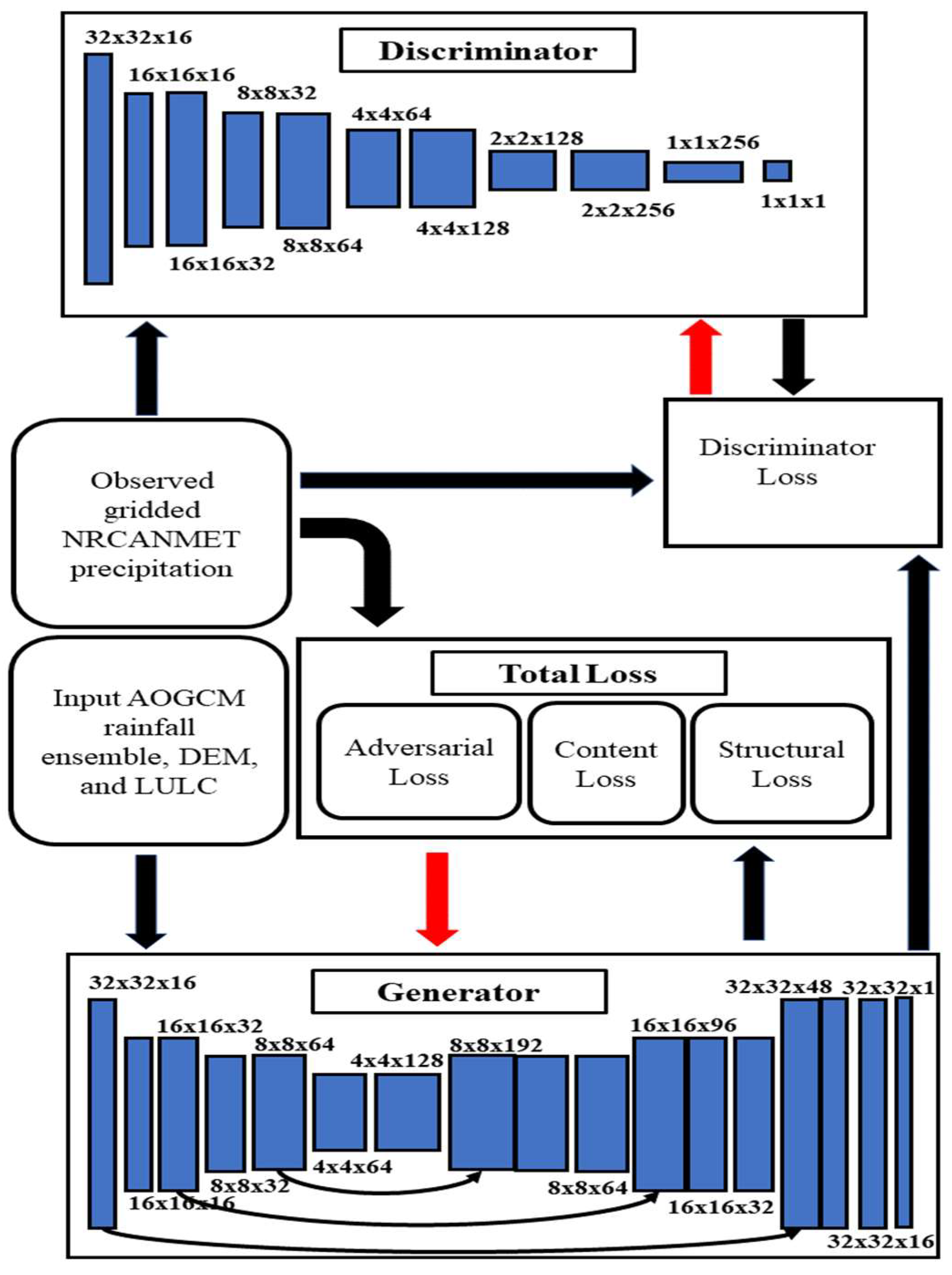
Generative network is developed into a U-net (Ronneberger et al. 2015) convolution-style encoder decoder with skipped link. LeakyReLu with momentum 0.2 was used for activating the hidden layers and for downsampling. In the last generator layer, ReLu has been used to provide positive output which is important for precipitation simulation.
A convolution encoder with a strided convolution downsampler is used as the discriminative network. We used LeakyReLu with momentum 0.2 as the activation function in the hidden layers and output layer is activated by a linear function. The approximate earth moving distance (Wasserstein distance) between the observed and simulated precipitation is calculated by the discriminator. We have built a compact support for layer weights by cutting them between [-0.1, 0.1] following recommended parameterization for WGAN models.
The schematic for the networks and training procedure are shown in
Figure 4. The black arrows indicate the flow of data and red arrows indicate the feedback of objective functions to the models in terms of optimized parameters.
2.2.5. Training Details
The training was done on the 4000 GPU NVIDIA Quadro. Input / output data rescaling were avoided in any way and the model was able to learn and evolve the climate signal present in the various model datasets and observations. Optimization of the generator was done using the Linf norm (Adamax) (Ruder et. al. 2016) Adam gradient-base optimization, with initial learning rate 0.02 and decay 0.5. We wanted the discriminator to calculate the gradient in the current iteration based on an adaptive window and did not want to use the previous gradient data generator results. We used the Adam (Adadelta) moving window update (Zeiler et. al. 2012) to train the Wasserstein distance computer, discriminator. The model was trained for 15,000 iterations which are more than sufficient to simulate high-resolution realistic precipitation patterns. With just 10,000 iterations, even the error stabilized.
3. Results
The temporal median for different AOGCMs is shown in figures S2-S10. In these plots (inter-model uncertainty) the diverse nature of spatial patterns and variabilities in their magnitudes is prominent (Chen et. al. 2014). The correction of these biases (or differences) with respect to the observed patterns is a prominent objective in downscaling these precipitations over any location (Manzanas et. al. 2018). An ideal downscaling method not only makes the realization of any climatic variable to higher resolution at regional level, but these patterns and magnitude should also be corrected to produce the spatial and temporally coherent observed climate distribution.
Table 3 shows the sensitivities of different model input and loss functions. The model is run with different combinations and the minimum error statistics in last 50 iterations are shown in the table. The model with no LULC and DEM as input shows NS of 0.0020 and DSSIM of 0.0118, with only DEM input the NS is 0.0013 and DSSIM is 0.0098, with only LULC as input the NS is 0.0018 and DSSIM is 0.0099, and with both DEM and LULC as input the NS is around 0.0012 and DSSIM is around 0.0098. This signifies that the DEM is a major driver for regional climate. The LULC may not be as significant as the DEM in altering the extreme rainfall. We speculate the non-time varying input LULC data can also attribute to its lower performance. However, due to unavailability of quality LULC data, we could not test that hypothesis. Furthermore, we ran the same model with both LULC and DEM as input but with MAE and NS as loss function. The resultant NSs are 0.0030 and 0.0021, respectively and DSSIMs are 0.0355 and 0.0517, respectively. This signifies the superiority of the total error formulation compared to the traditional point-based loss functions.
To understand the effect of the site-specific DEM and LULC in details we analyzed the Mean Absolute Percentage Error (MAPE) for different input types at different sites in
Table 4. The result shows the heterogeneous loss relative to the location-specific geographic attributes. The inclusion of the DEM as one of the inputs improved the loss estimate at all the sites. The average MAPE over all the sites decreased from 2.64% to 1.49%. However, even though the average MAPE decreased from 2.64% to 1.78% which is consistent for all the sites except one, the response of the LULC input deteriorated over Yellowknife. At several sites, the inclusion of the LULC deteriorated the results compared to DEM only input (
Table 4). It has improved the loss estimate where majority of the LULC are expected to the constant in time such as Goose Bay or Yellowknife which are located on water bodies and Calgary which is located in a transition zone between coniferous high mountain forest to the west and prairie plains to the east. However, at other sites removal of forest cover or expansion of urban land cover might create dynamic interactions between climate and landcover that conflicts with the assumption of static LULC as input used in the model impacting model performance The further verification of this hypothesis is out of scope of this paper and due to unavailability of the long-term LULC data for these regions, we could not verify this hypothesis.
Table 3.
Sensitivities of different model inputs and settings to the output of the model after 10,000 iterations. We have taken the minimum statistics of the last 50 iterations.
Table 3.
Sensitivities of different model inputs and settings to the output of the model after 10,000 iterations. We have taken the minimum statistics of the last 50 iterations.
| Model setting |
NS |
DSSIM |
| No LULC and DEM input |
0.0020 |
0.0118 |
| Only DEM input |
0.0013 |
0.0098 |
| Only LULC input |
0.0018 |
0.0099 |
| LULC and DEM inputs |
0.0012 |
0.0098 |
| MAE loss function with LULC and DEM inputs |
0.0030 |
0.0355 |
| NS loss function with LULC and DEM inputs |
0.0021 |
0.0517 |
Table 4.
Effect of different types of inputs on the simulation performance.
Table 4.
Effect of different types of inputs on the simulation performance.
| |
No LULC and DEM inputs |
Only DEM input |
Only LULC input |
Both LULC and DEM inputs |
| Schefferville |
2.49 |
0.90 |
1.30 |
1.04 |
| Goose Bay |
3.12 |
1.21 |
1.17 |
0.93 |
| Yellowknife |
3.14 |
2.76 |
3.84 |
1.78 |
| Edmonton |
2.45 |
1.10 |
1.30 |
1.31 |
| Calgary |
2.39 |
1.89 |
1.86 |
1.75 |
| Saskatoon |
2.37 |
1.18 |
1.58 |
1.23 |
| Regina |
2.52 |
1.22 |
1.41 |
1.36 |
| Average |
2.64 |
1.46 |
1.78 |
1.34 |
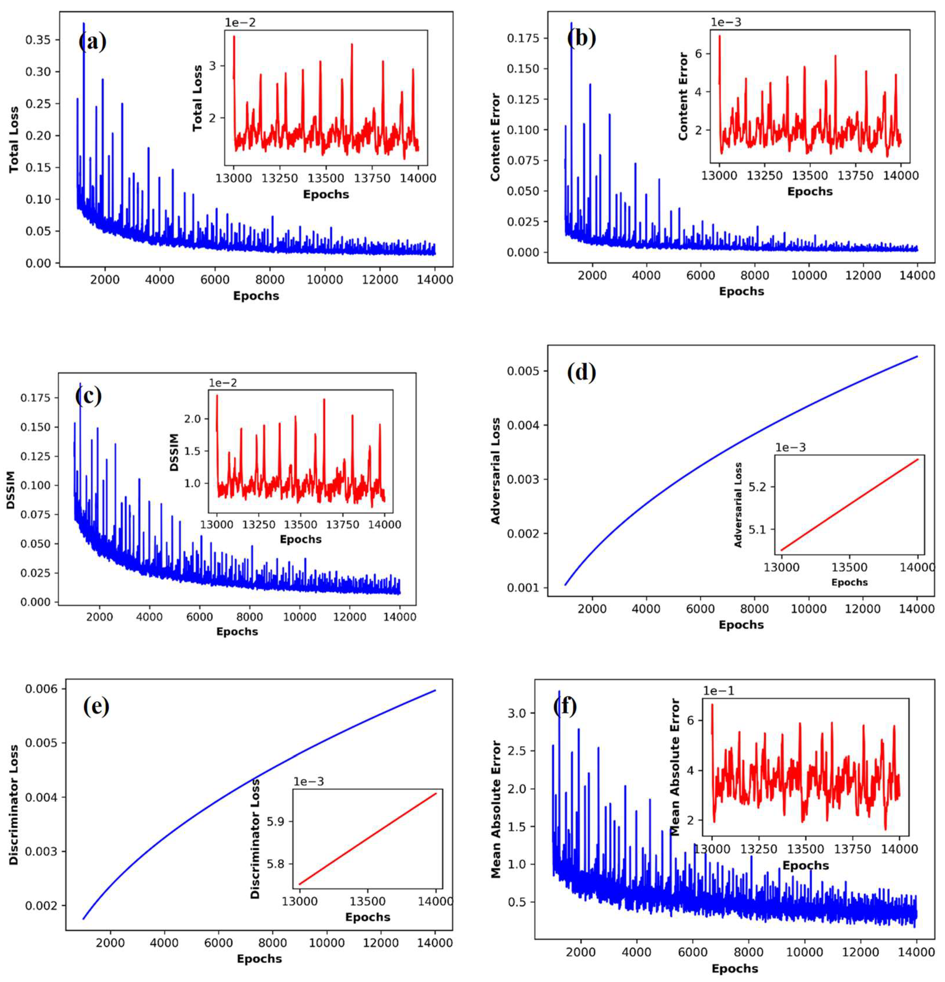
In our finalized simulation we discarded the initial 1000 iteration recording as a spin up of the model and showed 1000 to 15,000 model diagnostics in
Figure 5.
Figure 5a shows the total loss of the downscaling. Notice, the error almost stabilizes after 10,000 iterations. We describe the minimum of last 50 iterations here. The total error after 15,000 iterations is around 0.013. Considering this is a combination of 3 types of errors, (i.e., adversarial error, content error, and structural error), it does not have any meaningful unit.
Figure 5b shows the content loss almost stabilized around a value 0.0012 after 15,000 iterations.
Figure 5c shows the structural loss almost stabilized around a value of 0.007. However, the adversarial loss in
Figure 5d keeps on increasing after 15,000 iterations has a value of 0.0054. This signifies the discriminator can still resolve the differences between the observed and predicted precipitation patterns.
Figure 5e shows the discriminator error. It also keeps on increasing, signifying good performance of the generator. However, the loss of the discriminator 0.0061 is higher than the adversarial error. As an extra diagnostic we also tracked widely used loss metric mean absolute error.
Figure 5f shows the trace of mean absolute error which stabilized around a value of 0.29 mm/day after 15,000 iterations.
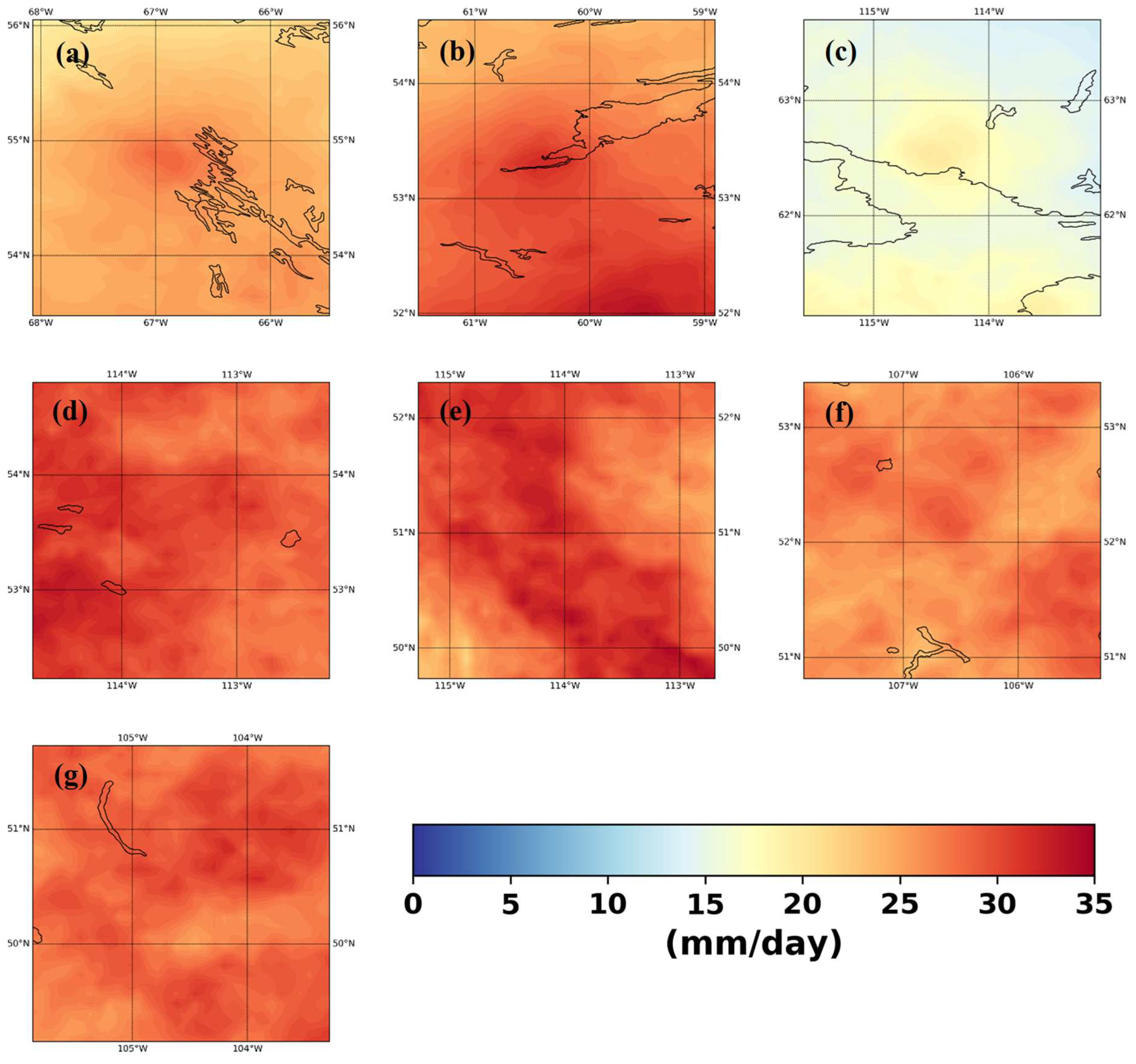
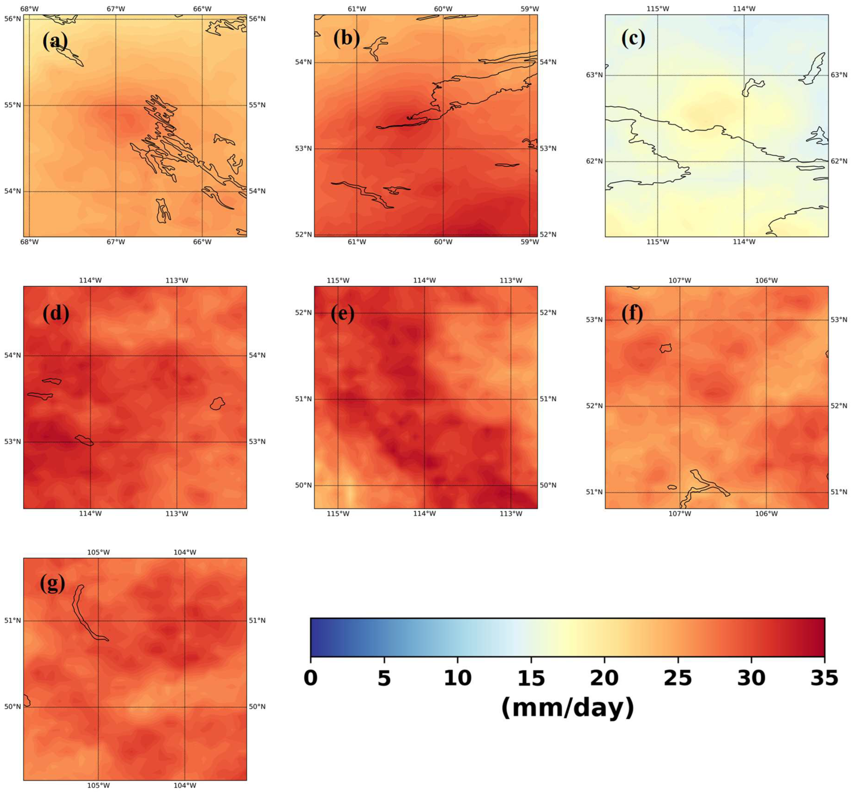
Figure 6 and
Figure 7 show the temporal median of observed (
Figure 6) and downscaled (
Figure 7) annual maximum precipitation. The regional patterns are well captured by the model. Notice, the spread of high rainfall around the cities (middle point of the region of interest). We presume this is an artifact of the interpolation method used to create the gridded precipitation data. This effect is prominent for the regions where the station density is especially low, (e.g., Yellowknife) (
Figure 6c). However, the simulated rainfall can pick up this artefact as well regardless of the somewhat questionable accuracy of the precipitation around these regions.
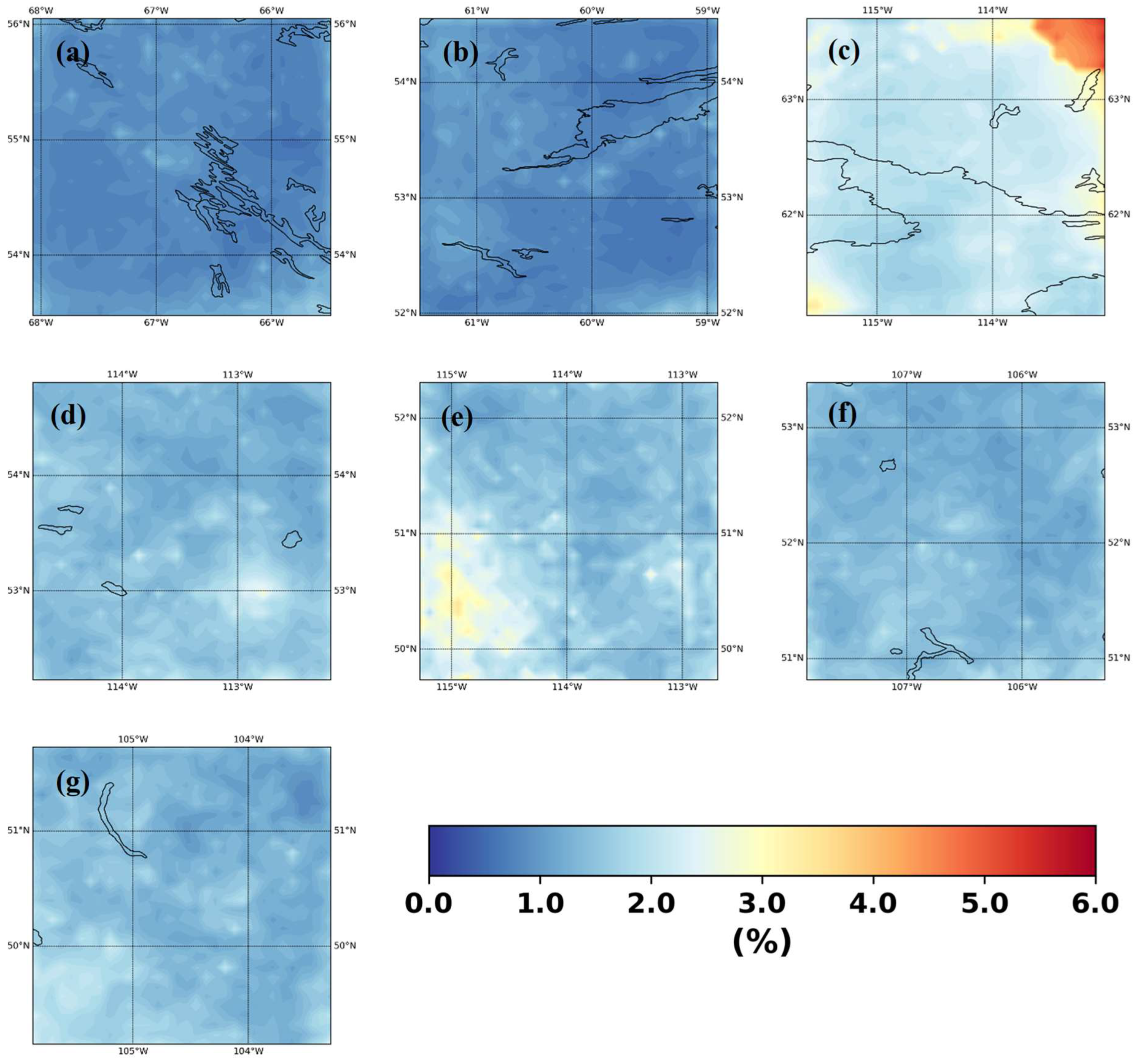
We calculated several error diagnostics of the downscaling performance to help us in understanding the regional, topographic, LULC effects on downscaling.
Figure 8 shows the temporal mean absolute percent error. The maximum error is around 6%, however this error is mostly confined to the north-eastern part of the Yellowknife which may be attributed to the uncertain land-cover and south-western part of Calgary where the region has more variable topography. We think this is due to the interaction of orographic or land cover features in this region attributed to this high percent error. Figure S11 shows the temporal correlation between the observed and downscaled precipitation. The minimum correlation is 0.95 which is well beyond the acceptable limit. However, like the error behavior this low correlation is concentrated over the north-eastern part of Yellowknife. For other regions, the minimum correlation is more than 0.99. Figure S12 shows the p-values of the Kolmogorov-Smirnov test for equivalency of temporal distribution of observed and downscaled annual maximum. The plots indicate that we cannot reject the equivalency of the distributions between the observed and downscaled (null hypothesis) at 90% confidence limit for most of the regions apart from a small region in the south-western Calgary attributed to its orographic features and few other disjointed small regions. However, we think the model should be able to overcome this problem as well with extended training periods.
Figure 7.
Median downscaled annual maximum daily precipitation for (a) Schefferville, (b) Goose Bay, (c) Yellowknife, (d) Edmonton, (e) Calgary, (f) Saskatoon, (g) Regina.
Figure 7.
Median downscaled annual maximum daily precipitation for (a) Schefferville, (b) Goose Bay, (c) Yellowknife, (d) Edmonton, (e) Calgary, (f) Saskatoon, (g) Regina.
Figure 8.
Mean Absolute Percentage Error between downscaled and observed precipitation for (a) Schefferville, (b) Goose Bay, (c) Yellowknife, (d) Edmonton, (e) Calgary, (f) Saskatoon, (g) Regina.
Figure 8.
Mean Absolute Percentage Error between downscaled and observed precipitation for (a) Schefferville, (b) Goose Bay, (c) Yellowknife, (d) Edmonton, (e) Calgary, (f) Saskatoon, (g) Regina.
4. Discussion
The modeling results presented here demonstrate that our downscaling methodology can effectively downscale AOGCM precipitation extremes to a regional scale product. This methodology is a novel extension of a recently developed downscaling computational framework based on GAN. In this paper we extend this new framework by incorporating site-specific covariates that describe localized information about the downscaling relationship. Further, the use of multiple loss functions was found to have a significant impact on downscaling results across the domains investigated here.
The key conclusions from our study are summarized as follows. Firstly, the MSCliGAN framework can utilize diverse information present in different AOGCM simulations, topography, and land-use/land-cover to create a spatially coherent field close to observation data. The approach is similar in concept to Reliability Ensemble Averaging (REA) conceptualized by Girogi et. al., 2001 using a CNN and adversarial training context for multiple sites. Our model demonstrates good performance for downscaling extreme precipitation which is generally considered less predictable than mean climate/precipitation (Haylock et. al. 2006; Frei et al. 2006; Hundecha et. al. 2008).
The use of topography and LULC ensure the embedded regional characteristics of the precipitation and can demonstrate the struggles of the models over the regions of diverse topography. Apparent interactions of LULC are also prominent in the model output. Topography was found to be the most important driver for regulating regional extreme precipitation patterns. The importance of LULC is somewhat inconclusive due to unavailability of good quality time varying LULC data. The SSIM index enabled us to get the probing ability into the model regional characteristics and proves that the only point-based error functions which are popular in traditional statistical downscaling, are not sufficient to reliably reproduce the regional characteristics. The use of total loss function which is a summation of content, structural, and adversarial losses can lead to higher quality downscaled products. The adversarial loss can provide a justifiable gradient to the weight optimization in cases where traditional loss functions fail and oscillates in near convergence variabilities.
In order to further investigate this approach, we should use time-varying LULC as input and estimate its sensitivity with respect to simulation performance. The current generator architecture is not efficient in a sense that it requires the input AOGCM precipitation to be interpolated to the output grid. It is possible develop a more efficient architecture where the input will start at its native resolution and subsequently get finer to reach the target resolution. We think by incorporating static inputs such as topography and LULC at different resolution, this will result in more structurally realistic simulation. More research is needed to understand the structural error. Understanding and devising more indices such as snow water equivalent obtained from passive microwave sensing would enable us to understand the regional structures of the climatic variables, how the static topography and LULC interact with them and thus would improve the subsequent simulation. Another, research direction would be improving the ML-techniques to incorporate the time dimension. In the current approach the annual maximum daily rainfall is treated as temporally independent samples. Incorporation of the temporal dimension in the simulation would thus produce more realistic results.
These results offer significant potential for fields investigating the impacts of climate change and climate processes. The mismatch between the scales of AOGCMs and spatial scales at the level of impacts (e.g., hydrological, ecological, economic), makes it difficult to assess direct relationships and outcomes. Downscaling methods help bridge this breach by making climate model information more meaningful and useful to scientists working on a more localized geographical scale across disciplines. Incorporating topographic, land use-land cover information, and local structure of the variable of interest in the training of CNN-based downscaling models, this study reveals that observational gridded data for maximum yearly rainfall are replicated in several region of interest in Canada, with various level of collected station data and where climate change information is very important. To benefit the scientific community more widely, further work is needed to develop and evaluate the MSCliGAN modelling framework in different geographical and thematic contexts.
Author Contributions
The idea behind this research was conceived, implemented, and written equally by both authors.
Funding
This work was funded in part by the Global Water Futures research programme.
Data Availability Statement
Any data that support the findings of this study and the custom code used in this study, not already publicly available, are available from the corresponding author, C. Chaudhuri, upon reasonable request.
Conflicts of Interest
The authors declare that there are no competing interests.
References
- Arjovsky, M.; Chintala, S.; Bottou, L. Wasserstein gan. arXiv 2017, arXiv:1701.07875. [Google Scholar]
- Canada Centre for Remote Sensing. 2015 Land Cover of Canada (Record ID 4e615eae-b90c-420b-adee-2ca35896caf6). [Data set]. Natural Resources Canada. 2019. Available online: https://open.canada.ca/data/en/dataset/4e615eae-b90c-420b-adee-2ca35896caf6.
- Carpenter, S.R.; Booth, E.G.; Kucharik, C.J. Extreme precipitation and phosphorus loads from two agricultural watersheds. Limnol. Oceanogr. 2018, 63, 1221–1233. [Google Scholar] [CrossRef]
- Castellano, C.M.; DeGaetano, A.T. A multi-step approach for downscaling daily precipitation extremes from historical analogues. Int. J. Clim. 2016, 36, 1797–1807. [Google Scholar] [CrossRef]
- Chaudhuri, C.; Srivastava, R. A novel approach for statistical downscaling of future precipitation over the Indo-Gangetic Basin. J. Hydrol. 2017, 547, 21–38. [Google Scholar] [CrossRef]
- Chaudhary, S.; Agarwal, A.; Nakamura, T. Rainfall Projection in Yamuna River Basin, India, Using Statistical Downscaling, Water Resources and Environmental Engineering II; Springer, 2019; pp. 15–23. [Google Scholar] [CrossRef]
- Chen, H.; Xu, C.-Y.; Guo, S. Comparison and evaluation of multiple GCMs, statistical downscaling and hydrological models in the study of climate change impacts on runoff. J. Hydrol. 2012, 434, 36–45. [Google Scholar] [CrossRef]
- Chen, H.; Sun, J.; Chen, X. Projection and uncertainty analysis of global precipitation-related extremes using CMIP5 models. Int. J. Clim. 2014, 34, 2730–2748. [Google Scholar] [CrossRef]
- Cho, J.; Oh, C.; Choi, J.; Cho, Y. Climate change impacts on agricultural non-point source pollution with consideration of uncertainty in CMIP5. Irrig. Drain. 2016, 65, 209–220. [Google Scholar] [CrossRef]
- Kingma, D.P.; Ba, J. Adam: A Method for Stochastic Optimization. In Proceedings of the 3rd International Conference on Learning Representations (ICLR); 2014. [Google Scholar] [CrossRef]
- Dong, C.; Loy, C.C.; He, K.; Tang, X. Learning a Deep Convolutional Network for Image Super-Resolution. In Computer Vision–ECCV 2014. ECCV 2014. Lecture Notes in Computer Science; Fleet, D., Pajdla, T., Schiele, B., Tuytelaars, T., Eds.; Springer: Cham, 2014; Volume 8692. [Google Scholar] [CrossRef]
- Eekhout, J.P.C.; Hunink, J.E.; Terink, W.; de Vente, J. Why increased extreme precipitation under climate change negatively affects water security. Hydrol. Earth Syst. Sci. 2018, 22, 5935–5946. [Google Scholar] [CrossRef]
- Frei, C.; Schöll, R.; Fukutome, S.; Schmidli, J.; Vidale, P.L. Future change of precipitation extremes in Europe: Intercomparison of scenarios from regional climate models. J. Geophys. Res. Atmos. 2006, 111. [Google Scholar] [CrossRef]
- GEBCO Compilation Group. GEBCO 2019 Grid. 2019. [CrossRef]
- Ghosh, S.; Mujumdar, P. Statistical downscaling of GCM simulations to streamflow using relevance vector machine. Adv. Water Resour. 2008, 31, 132–146. [Google Scholar] [CrossRef]
- Giorgi, F.; Mearns, L.O. Probability of regional climate change based on the Reliability Ensemble Averaging (REA) method. Geophys. Res. Lett. 2003, 30. [Google Scholar] [CrossRef]
- Goodfellow, I.; Pouget-Abadie, J.; Mirza, M.; Xu, B.; Warde-Farley, D.; Ozair, S.; Courville, A.; Bengio, Y. Generative adversarial nets. Advances in Neural Information Processing Systems (NIPS) 2014, 3, 2672–2680. [Google Scholar]
- Haylock, M.R.; Cawley, G.C.; Harpham, C.; Wilby, R.L.; Goodess, C.M. Downscaling heavy precipitation over the United Kingdom: a comparison of dynamical and statistical methods and their future scenarios. Int. J. Clim. 2006, 26, 1397–1415. [Google Scholar] [CrossRef]
- Hidalgo, H.G.; Dettinger, M.D.; Cayan, D.R. Downscaling with constructed analogues: daily precipitation and temperature fields over the United States. In California Energy Commission PIER Final Project Report CEC-500-2007-123; 2008. [Google Scholar]
- Hirabayashi, Y.; Mahendran, R.; Koirala, S.; Konoshima, L.; Yamazaki, D.; Watanabe, S.; Kim, H.; Kanae, S. Global flood risk under climate change. Nat. Clim. Chang. 2013, 3, 816–821. [Google Scholar] [CrossRef]
- Hundecha, Y.; Bárdossy, A. Statistical downscaling of extremes of daily precipitation and temperature and construction of their future scenarios. Int. J. Clim. 2008, 28, 589–610. [Google Scholar] [CrossRef]
- Hutchinson, M.F.; McKenney, D.W.; Lawrence, K.; Pedlar, J.H.; Hopkinson, R.F.; Milewska, E.; Papadopol, P. Development and Testing of Canada-Wide Interpolated Spatial Models of Daily Minimum–Maximum Temperature and Precipitation for 1961–2003. J. Appl. Meteorol. Clim. 2009, 48, 725–741. [Google Scholar] [CrossRef]
- Huth, R. Statistical Downscaling of Daily Temperature in Central Europe. J. Clim. 2002, 15, 1731–1742. [Google Scholar] [CrossRef]
- Kioutsioukis, I.; Melas, D.; Zanis, P. Statistical downscaling of daily precipitation over Greece. Int. J. Clim. 2008, 28, 679–691. [Google Scholar] [CrossRef]
- Krizhevsky, A.; Sutskever, I.; Hinton, G.E. Imagenet classification with deep convolutional neural networks. In Advances in neural information processing systems; 2012; pp. 1097–1105. [Google Scholar]
- Lecun, Y.; Bottou, L.; Bengio, Y.; Haffner, P. Gradient-based learning applied to document recognition. Proc. IEEE 1998, 86, 2278–2324. [Google Scholar] [CrossRef]
- Lee, S.-S.; Moon, J.-Y.; Wang, B.; Kim, H.-J. Subseasonal Prediction of Extreme Precipitation over Asia: Boreal Summer Intraseasonal Oscillation Perspective. J. Clim. 2017, 30, 2849–2865. [Google Scholar] [CrossRef]
- Li, Z.; et al. Non-point source pollution changes in future climate scenarios: a case study of Ashi River, China. Fresenius Environ. Bull. 2017, 26, 6621–6631. [Google Scholar]
- Manzanas, R.; Lucero, A.; Weisheimer, A.; Gutiérrez, J.M. Can bias correction and statistical downscaling methods improve the skill of seasonal precipitation forecasts? Clim. Dyn. 2018, 50, 1161–1176. [Google Scholar] [CrossRef]
- Maraun, D.; Wetterhall, F.; Ireson, A.M.; Chandler, R.E.; Kendon, E.J.; Widmann, M.; Brienen, S.; Rust, H.W.; Sauter, T.; Themeßl, M.; et al. Precipitation downscaling under climate change: Recent developments to bridge the gap between dynamical models and the end user. Rev. Geophys. 2010, 48, 1–34. [Google Scholar] [CrossRef]
- Zeiler, M.D. ADADELTA: An Adaptive Learning Rate Method. arXiv 2012, arXiv:1212.5701. [Google Scholar] [CrossRef]
- Murphy, J.M.; Sexton, D.M.H.; Barnett, D.N.; Jones, G.S.; Webb, M.J.; Collins, M.; Stainforth, D.A. Quantification of modelling uncertainties in a large ensemble of climate change simulations. Nature 2004, 430, 768–772. [Google Scholar] [CrossRef]
- Plouffe, C.C.; Robertson, C.; Chandrapala, L. Comparing interpolation techniques for monthly rainfall mapping using multiple evaluation criteria and auxiliary data sources: A case study of Sri Lanka. Environ. Model. Softw. 2015, 67, 57–71. [Google Scholar] [CrossRef]
- Raghavendra, A.; Dai, A.; Milrad, S.M.; Cloutier-Bisbee, S.R. Floridian heatwaves and extreme precipitation: future climate projections. Clim. Dyn. 2018, 52, 495–508. [Google Scholar] [CrossRef]
- Ronneberger, O.; Fischer, P.; Brox, T. U-Net: Convolutional Networks for Biomedical Image Segmentation. In Proceedings of the 18th International Conference, Munich, Germany, 5–9 October 2015. [Google Scholar] [CrossRef]
- SHI, X.; Chen, Z.; Wang, H.; Yeung, D.-Y.; Wong, W.; WOO, W. Convolutional LSTM Network: A Machine Learning Approach for Precipitation Nowcasting. In Advances in Neural Information Processing Systems 28; Cortes, C., Lawrence, N.D., Lee, D.D., Sugiyama, M., Garnett, R., Eds.; Curran Associates, Inc., 2015; pp. 802–810. Available online: http://papers.nips.cc/paper/5955-convolutional-lstm-network-a-machine-learning-approach-for-precipitation-nowcasting.pdf.
- Tryhorn, L.; DeGaetano, A. A comparison of techniques for downscaling extreme precipitation over the Northeastern United States. Int. J. Clim. 2011, 31, 1975–1989. [Google Scholar] [CrossRef]
- Trzaska, Sylwia & Schnarr, Emilie. A Review of Downscaling Methods for Climate Change Projections. 2014.
- Wang, Q.; Yuan, Z.; Du, Q.; Li, X. GETNET: A General End-to-End 2-D CNN Framework for Hyperspectral Image Change Detection. IEEE Trans. Geosci. Remote Sens. 2019, 57, 3–13. [Google Scholar] [CrossRef]
- Weichert, A.; Bürger, G. Linear versus nonlinear techniques in downscaling. Clim. Res. 1998, 10, 83–93. [Google Scholar] [CrossRef]
- Wetterhall, F.; Halldin, S.; Xu, C.-Y. Statistical precipitation downscaling in central Sweden with the analogue method. J. Hydrol. 2005, 306, 174–190. [Google Scholar] [CrossRef]
- Widmann, M.; Bretherton, C.S.; Salathé, E.P., Jr. Statistical precipitation downscaling over the northwestern United States using numerically simulated precipitation as a predictor. J. Clim. 2003, 16, 799–816. [Google Scholar] [CrossRef]
- Wilby, R.L.; Wigley, T.M.L.; Conway, D.; Jones, P.D.; Hewitson, B.C.; Main, J.; Wilks, D.S. Statistical downscaling of general circulation model output: A comparison of methods. Water Resour. Res. 1998, 34, 2995–3008. [Google Scholar] [CrossRef]
- Wilby, R.L.; Harris, I. A framework for assessing uncertainties in climate change impacts: Low-flow scenarios for the River Thames, UK. Water Resour. Res. 2006, 42. [Google Scholar] [CrossRef]
- Xu, C.-Y. From GCMs to river flow: a review of downscaling methods and hydrologic modelling approaches. Prog. Phys. Geogr. 1999, 23, 229–249. [Google Scholar] [CrossRef]
- Yhang, Y.-B.; Sohn, S.-J.; Jung, I.-W. Application of Dynamical and Statistical Downscaling to East Asian Summer Precipitation for Finely Resolved Datasets. Adv. Meteorol. 2017, 2017, 1–9. [Google Scholar] [CrossRef]
- Yi, C.; Shin, Y.; Roh, J.-W. Development of an Urban High-Resolution Air Temperature Forecast System for Local Weather Information Services Based on Statistical Downscaling. Atmosphere 2018, 9, 164. [Google Scholar] [CrossRef]
- Zhang, J.; Craigmile, P.F.; Cressie, N. Loss Function Approaches to Predict a Spatial Quantile and Its Exceedance Region. Technometrics 2008, 50, 216–227. [Google Scholar] [CrossRef]
- Zhao, P.; Lü, H.; Yang, H.; Wang, W.; Fu, G. Impacts of climate change on hydrological droughts at basin scale: A case study of the Weihe River Basin, China. Quat. Int. 2019, 513, 37–46. [Google Scholar] [CrossRef]
- Zorita, E.; von Storch, H. The analog method as a simple statistical downscaling technique: comparison with more complicated methods. J. Clim. 1999, 12, 2474–2489. [Google Scholar] [CrossRef]
|
Disclaimer/Publisher’s Note: The statements, opinions and data contained in all publications are solely those of the individual author(s) and contributor(s) and not of MDPI and/or the editor(s). MDPI and/or the editor(s) disclaim responsibility for any injury to people or property resulting from any ideas, methods, instructions or products referred to in the content. |
© 2023 by the authors. Licensee MDPI, Basel, Switzerland. This article is an open access article distributed under the terms and conditions of the Creative Commons Attribution (CC BY) license (http://creativecommons.org/licenses/by/4.0/).
