1. Introduction
The aggregated modeling of urban networks has a long history dating back to [
1], and numerous theories and models have been published since; see [
2] for a recent review and reference therein. The starting point for all macroscopic urban models is the reservoir (or bathtub) model for cities, which simply states the conservation of
, the number of vehicles inside the network at time
t:
where
give the inflow and outflow of the network, respectively, in units of flow. The main assumption in these models is that the speed of vehicles inside the network at time
t,
, is identical for all vehicles and given by the speed macroscopic fundamental diagram (speed-MFD):
Unlike the inflow
, which can be easily determined, the network outflow
can be difficult to formalize due to its convoluted dependence on the probability distribution of trip lengths. Depending on the assumptions to formulate the outflow function
, the literature can be divided into accumulation-based [
3,
4,
5] and trip-based models [
6,
7,
8,
9,
10,
11,
12,
13,
14]. Accumulation-based models assume that the outflow is given by the network production divided by the average trip length,
ℓ:
This expression for the outflow was first derived in a seminal paper by [
3] only assuming a constant trip length and that congestion is evenly spread across the network. He points out that extracting dynamic behavior from the model is possible for slow-varying demands, providing the foundations for the macroscopic modeling of cities. Despite some confusion in the literature [
2,
15,
16,
17,
18], the role played by the exponential distribution in this model surfaced in the literature not until [
6] who considers it an unrealistic assumption. As it turns out, this important observation that (
3) follows from assuming exponentially distributed trip lengths, appears to have its origins in [
19] although it was not published until [
20] as described in [
15].
[
21] shows that the accumulation-based models suffer from significant numerical viscosity even when the time step is small. Outflows may then overreact to sudden demand surge leading to inconsistent information propagation between opposite perimeter boundaries. They also point out that the assumption of constant trip length for all vehicles inside a reservoir is not consistent with what is observed when the local dynamics are taken into account. This has prompted several extensions of the accumulation-based model, multi-reservoir systems with different categories of trip length over macroscopic routes, possibly changing with congestion levels, and delay-based models [
13,
22,
23,
24,
25,
26,
27,
28].
Trip-based reservoir models have been proposed that guarantee that all vehicles travel their own trip length, at the expense of mathematical tractability. Originally proposed by [
6] on a footnote, these models recognize that each commuter
i has different trip lengths,
, which has to equal the distance traveled inside the network during their trip time
at the prevailing speeds:
The resulting outflow function was proposed implicitly in [
9] without proof, arguing that it is a direct consequence of (
4) when the system is initially empty:
where
is the probability density of trip lengths of vehicles entering the network at time
s. [
15] introduces one spatial dimension to the problem,
x, the
remaining distance to reach the destination. He shows that when the distribution of trip lengths
f in (
5) is exponential with mean
ℓ, we obtain the accumulation-based model (
3), a result that first appeared in [
29]. All attempts in the literature to solve the trip-based model for other distributions have been numerical using discrete-event simulation [
9,
10,
11] or more traditional time-stepping simulation [
7]. Another advantage of trip-based models is the ease to incorporate slower vehicles such as buses [
18], although moving bottlenecks have been incorporated into the accumulation-based models [
30]. The interested reader is referred to [
12] for additional properties of accumulation-based and trip-based models under fast-varying demands.
To the best of our knowledge, with the exception of [
15], no other attempts have been made to develop analytical solutions to the trip-based model. To fill this gap, section 2 below uses the framework proposed in [
15] to derive analytical solutions of the trip-based model and to characterize its steady state, which coincides with the accumulation-based model independently of the trip-length distribution. Perhaps a more important gap in the literature is that the stochastic nature of arrival flows has been completely neglected, at least when it comes to analytical formulations; see [
2].
Section 3 fills this gap by drawing the analogy with the M/G/
∞ queue and shows that accumulations exhibit a much larger variance than predicted by the M/G/
∞ queue, due to the nonlinear dynamics imposed by the MFD. Finally, discussion and outlook are presented in section 4.
2. Jin’s Formulation: Alternative Derivation and Additional Results
The framework proposed in [
15] introduces one spatial dimension to the problem,
x, such that a vehicle trajectory
gives the
remaining distance to reach commuter
i’s destination, and
. By considering the probability density function of remaining trip distances, [
15] derives the conservation law that unifies existing reservoir models. Alternatively, one can simply note that these vehicle trajectories must obey the conservation law partial differential equation (PDE):
where
is the density of vehicles in the region at time
t whose remaining distance is
x,
is the corresponding flow, and the source term
is the net inflow to the system in units of flow per km. As opposed to regular traffic, in our problem
(i) there is no fundamental diagram relating flow to density and therefore (
6) it is not a hyperbolic conservation law such as the kinematic wave model. Instead, given assumption (
2) above, the flow is given by the fundamental traffic flow relationship:
which turns the conservation law (
6) into the transport PDE:
where the negative sign follows from
. Other important differences compared to regular traffic are that
(ii) the spacing between vehicle trajectories is immaterial because these vehicles could be in different links of the network;
(iii) only includes arrivals to the region because all departures take place at
. It follows from
(iii) that the outflow from the region is simply the flow at
, i.e.
, or equivalently using (
7)
1:
It follows that all we need to solve the model is
but unfortunately its analytical derivation quickly becomes intractable. For clarity, let
and the distance traveled by a vehicle during time interval
:
The initial value problem solution to the transport PDE (
8) is well known in the literature. Given initial densities
, the solution can be expressed as the following system of integral-differential equations:
which cannot be solved analytically in our case. However, it can be used to show the following:
Proposition 2.1. Lamotte and Geroliminis’s [
9] conjecture in (
5) can now be proven.
Proof. From (
13a) we see that for
and empty initial conditions:
which in combination with (
10) gives the desired result. □
2.1. Analytical Solutions for
Although (13) cannot be solved analytically for
, we have been able to find explicit solutions for
only for exponential and uniform trip length distributions under a time-independent conditions
and a Greenshields speed-accumulation relationship,
, where we assume that both the free-flow speed and jam accumulation are 1, without loss of generality. These assumptions imply that both the accumulation and time are dimensionless, measured in units of the jam accumulation and free-flow travel time, respectively. Let
the maximum outflow of the accumulation-based model:
and let the intensity be
, or:
In this case, one needs to solve the following system of equations:
subject to appropriate boundary conditions. When the distribution of trip lengths
f is exponential with mean
ℓ, one obtains the accumulation-based model (
3) as pointed out in [
15], and therefore one may replace (17a) and (17b) with (
1) and (
3), which removes the mathematical intractability of (17). With initial conditions
one obtains:
where
are constants; see
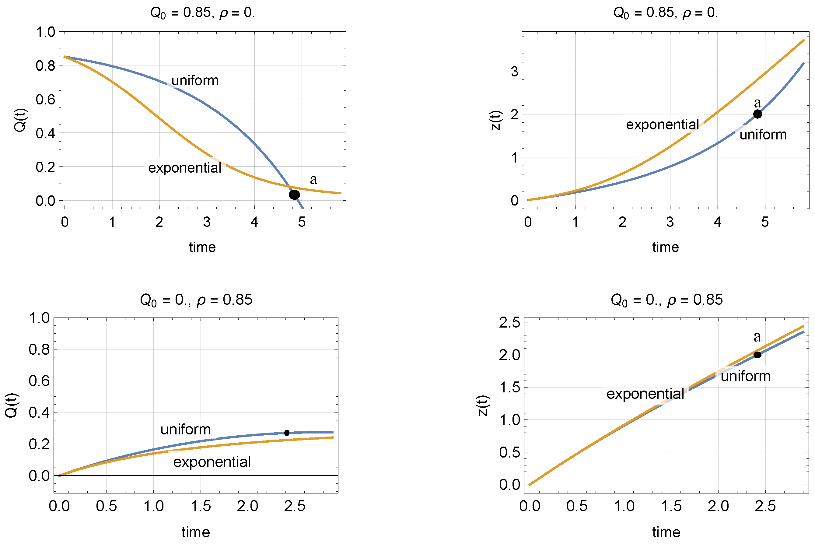
Figure 1. Notice that (21a) was presented in [
31] for occupancies, but the formulation here also allows us to obtain
. Other distributions of trip lengths did not result in analytical solutions of (17) (using Mathematica v13.1). The only exception is the uniform distribution, but in “relaxed” form:
instead of
, which is the uniform distribution in
with mean
ℓ. This relaxed form implies that the following analytical solutions are valid only up to a time
such that
. The general case
gives:
where here
,
,
,
. Notice that solution for
looks complicated and not particularly insightful, and therefore will be omitted in what follows; they can be easily retrieved using equation (17c). Two important special cases of (20) are arbitrary initial conditions and no inflow and empty initial conditions and constant inflow:
and are used to compare with the exponential disagree in
Figure 1. It can be seen in the first row of the figure that under uniform trip lengths the accumulation tends to zero much more slowly than in the exponential case for earlier times, while the opposite is true for later times. The second row shows an initially empty network being loaded at a constant intensity, where one can see that both distributions tend to the same equilibrium point but at slightly different speeds. Notice that models (18) and (21) are valid only in
, and as soon as we hit one of these boundaries one should stop the evaluation; see points “a” in the figure. Similarly, because we used the relaxed version of the uniform distribution, as soon as
then (21) no longer applies as noted earlier.
We can conclude that, given an average trip-length
ℓ, the effect of the trip-length distribution affects the time (as found in [
22]) to reach steady state, but not the equilibrium point itself. This is confirmed in the next section.
2.2. Steady-State
In this section all input variables are time-independent, i.e. , and all other steady-state variables denoted with a star.
Proposition 2.2 (Steady-state models). The accumulation-based model under steady-state conditions is valid regardless of the (time-independent) distribution of trip lengths.
Proof. In steady-state the network production
, defined as the integral of the circulating flow over the total network distance, has to match the incoming production
, therefore
where
. From (10) we can see that the steady-state condition
implies
as expected. Combining (23) and (22) gives:
which establishes the result. □
Notice that this proposition was mentioned in [
29] without proof. It implies that in steady state one may use the simple accumulation-based model to evaluate traffic conditions, regardless of the distribution of trip lengths. For instance, as shown previously in [
31], solving for
in (22) gives two equilibrium solutions; the first solution is stable and in the free-flow regime, and in the Greenshields approximation it reads as:
while the second solution,
, is in the congested regime and acts as a repellor; see [
31] for details.
Proposition 2.3 (Steady-state density). In steady-state, the density is given by:
Proof. In steady state, characteristics are straight lines of slope
, which means that the density
can be computed explicitly with the change of viable
to obtain:
Taking the limit
we obtain the steady-state density
as claimed. □
It follows that the probability density function (PDF) of remaining trip distances,
, is given by:
where
is the expected trip length. Denoting its coefficient of variation by
, it can be shown that their moments are given by [
32] as:
Notice that for the exponential distribution, (28) gives
, as expected given the memoryless property of this distribution
2. This means that the expected remaining trip length is
, as can be verified in (29) with
. For other distributions this is not the case, however, where
for distributions with light tails, as it appears to be the case in practice [
17,
33]. However, it would not be surprising to find cases where the trip length distribution is heavy tailed, such as the power-law distribution which is so prevalent in complex systems [
34], where
.
3. Queueing Approximation for the Stochastic Problem
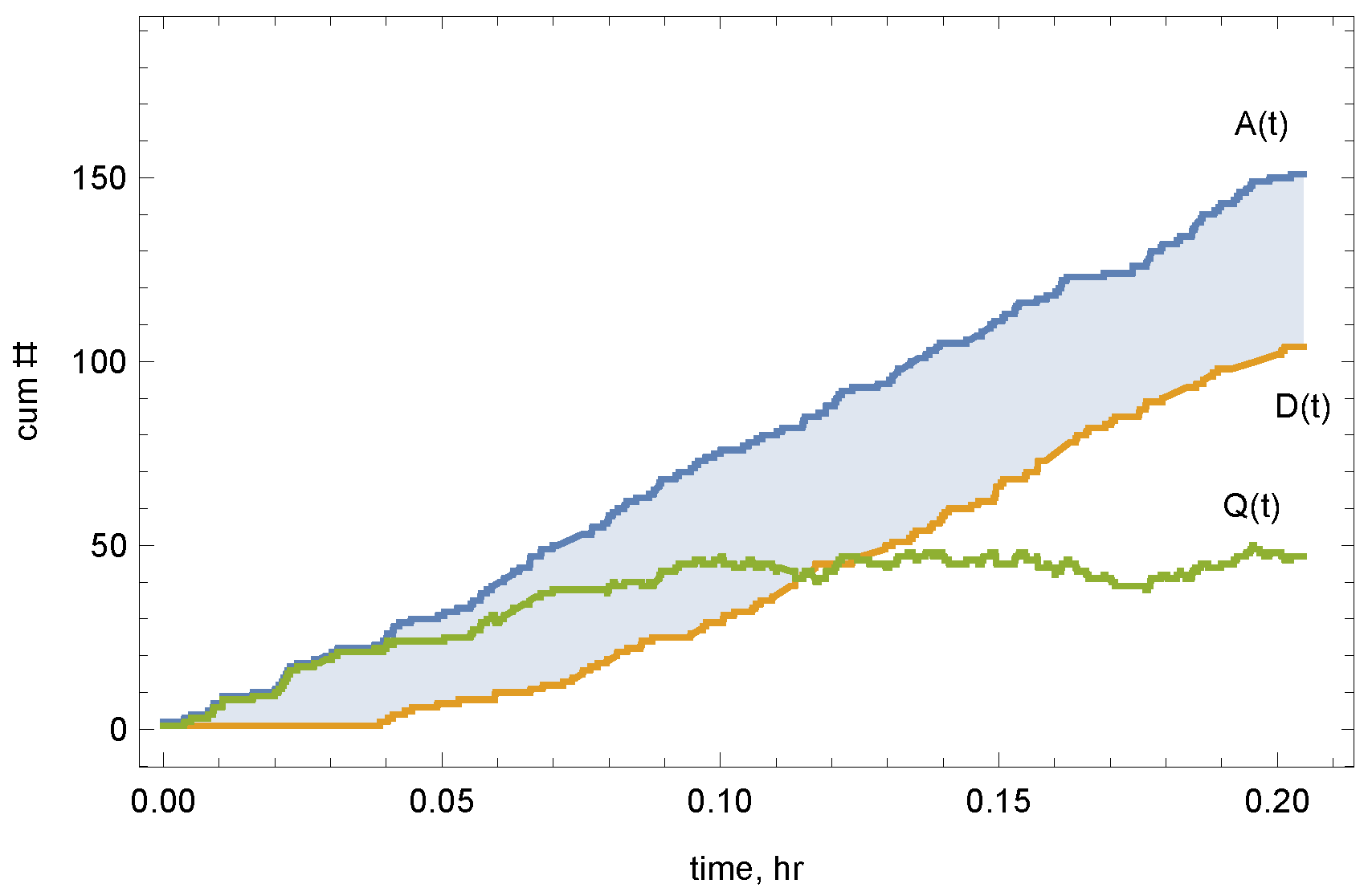
In this section, we present a queuing approximation for the stochastic version of our problem. For simplicity, we start with empty initial conditions and assume that the only sources of randomness are the arrival process and trip lengths, while the travel speed remains deterministic given the accumulation, as in the previous sections. The network accumulation (or queue)
is the difference between cumulative vehicle arrivals to the network,
, and departures from the network,
; see
Figure 2. The mean and variance of the accumulation is then given by:
In traditional queuing systems the departure rate is independent of the accumulation, which acts as a buffer between arrivals and departures: as long as the queue is not zero, departures tend to be independent of arrivals. As argued in [
35], the more the accumulation in the system, the more independent the departure and arrival process will be and is typically assumed that the covariance term
. This is true even for limited storage, which can be treated as a boundary condition. But in our case, by definition of the MFD there is a dependency between accumulation and service rate and therefore the covariance term
in (31b) cannot be neglected. In any case, as long as the accumulation is not close to zero, its distribution should be approximately normal with mean and variance given above; see [
35]. The challenge here is to characterize the terms
and
due to the nontrivial dependencies in the reservoir model.
As customary in the queueing literature, we introduce the variance-to-mean ratio of arrivals,
, departures,
, and accumulations,
:
Notice that
for Poisson arrivals, and that if service times are independent, then
gives the squared coefficient of variation of service times [
35], and equals one for exponential service times. It will be convenient to define:
which is one for the M/G/
∞ queue [
35], and is in the range
. With these definitions the variance-to-mean ratio of the accumulation can be written as:
which is the main focus of this section. Although this ratio is time dependent we will be interested in its state-state behavior in what follows.
The traditional queuing model most similar to our problem is the M/G/
∞ queue, with Poisson arrivals (so
), a general service time distribution, and an infinite number of servers. The latter means that each customer (commuter) is its own server and the service time plays the role of the travel time from origin to destination. The main difference with our problem is that travel times are governed by the reservoir model dynamics, and as it turns out, these dynamics will make a big difference: It is known that for the M/G/
∞ queue the distribution of departures is Poisson, so
and therefore accumulations are also Poisson, as can be seen in (34) that gives
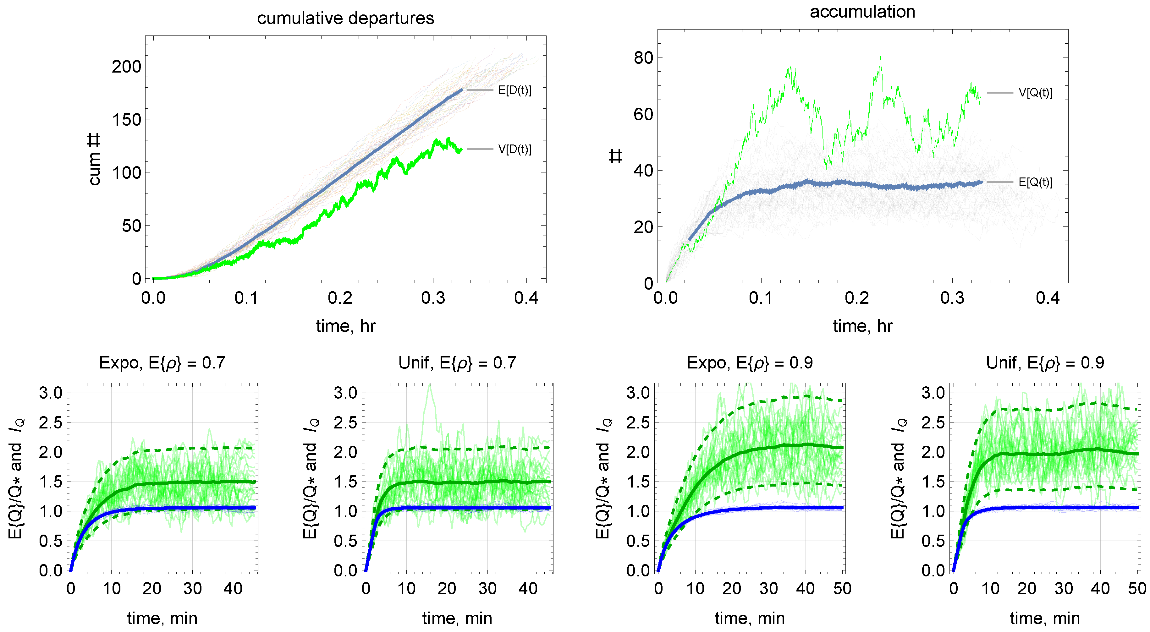
. But our discrete-event simulation (described in appendix) results presented in
Figure 3 and
Figure 4 show that
depending on the intensity
. The simulation experiments consider, separately, three trip-length distributions: exponential, uniform and the “square” distribution arising when origins and destinations are uniformly distributed on a square; see [
36]. The parameters of these distributions were set such that they all have the same mean, but different coefficient of variation: the
is 1, 1/27 and 1/4 for the exponential, uniform and square distribution, respectively.
Figure 3(Top) shows a typical simulation output in terms of cumulative count curves for departures (left) and accumulations (right) for several realizations of the experiment. Arrivals are omitted as they look very similar to the departure plot. From these outputs one can calculate the sample means of
,
, etc. to estimate the ratios
and
, all functions of time. The bottom part of the figure shows simulation time series showing the evolution of
and
with the exponential and uniform distributions for different values of
. It becomes clear that the distribution with the highest coefficient of variation, the exponential distribution, implies longer relaxation times to reach the steady state, but this steady state is unaffected by the distribution of trip lengths.
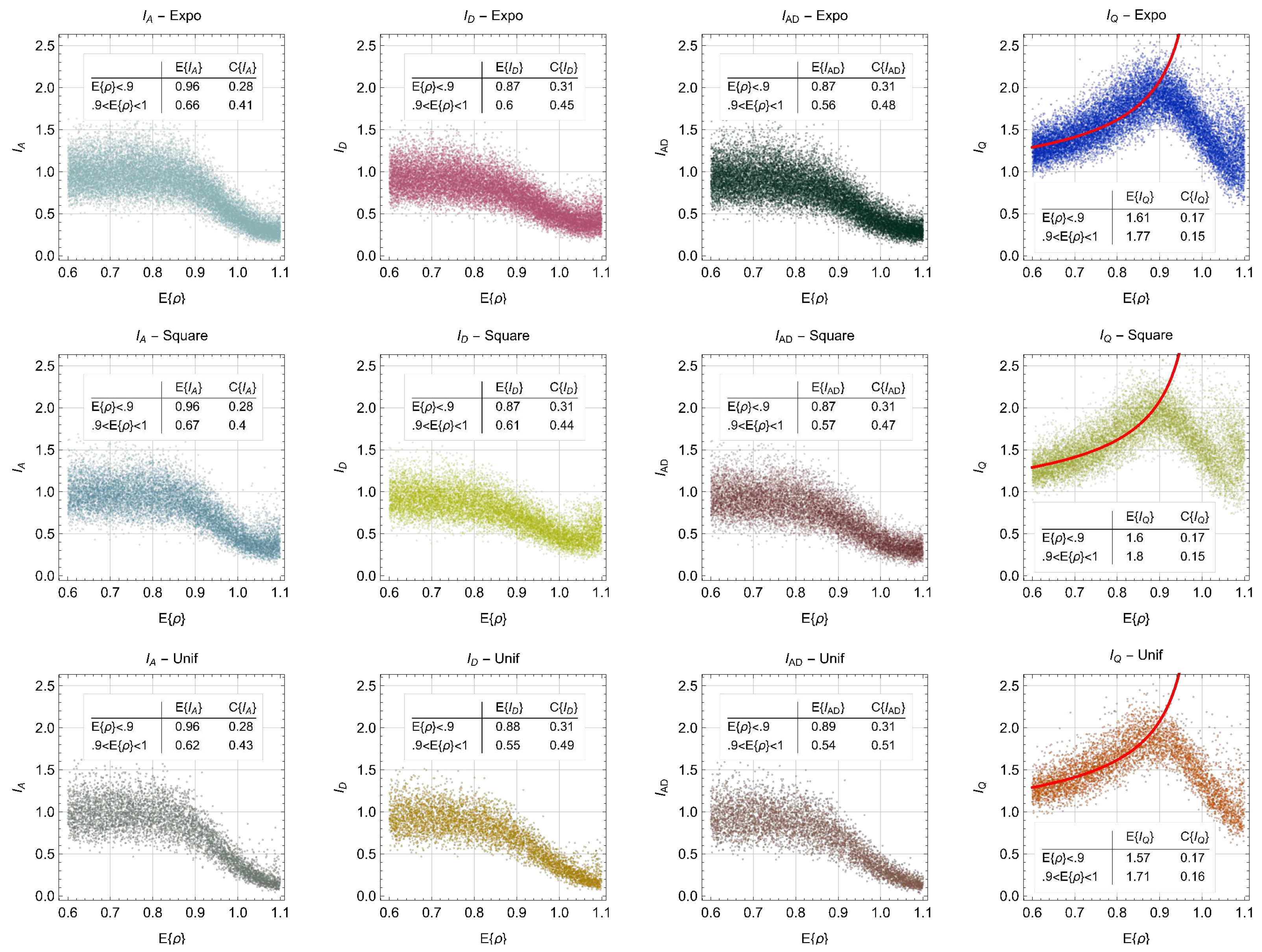
Figure 4 shows the steady-state time-average values of parameters
and
as a function of the average intensity
. It can be seen that all the columns in the figure look very similar, which indicates that the impact of the trip length distribution is almost negligible when it comes to the statistical properties of
and
. Notice that around intensity 0.9 there is a consistent drop in all the parameters, followed by a sudden increase at
. The drop is a consequence of arrival flows being throttled in congestion (see appendix), which causes a reduction in the variance of the relevant variables since the system is forced to maintain the same accumulation. The sudden increase can be explained by the non-stationary of the system when
. Notice that for
the first three columns of the figure are as expected, with
as we have Poisson arrivals, whose variability is dampened slightly due to the interactions in the bathtub, leading to smaller
and
.
Figure 4.
Steady-state time-average values of parameters and as a function of the intensity . Each row corresponds to a different distribution of trip length: exponential, uniform and square distribution. The red line corresponds to (36). The table on each panel gives the expected value and coefficient of variation of the relevant parameter for two ranges of .
But not as expected is the behavior of
observed in the last column of
Figure 4, which is not captured by (34). As shown next, this can be explained by the reservoir dynamics brought about by the MFD causing the variance to diverge to infinity near the critical point
. (Notice that this is not the case for the M/G/
∞ queue because it has no exit capacity constraint such as
here; see (15).) To see this, we series expand (25) around the critical point
up to first order and compute its variance assuming Poisson arrivals, i.e.
. This gives
, which goes to infinity as
. This behavior is typical of systems that undergo a phase transition [
37], e.g. from liquid to solid or from free-flow to congestion in our case. The usual way to deal with this divergence in the phase transition literature is to assume a power-law divergence, in this case of the type:
where
are constants and
b is known as a critical exponent. Assuming
we can compute:
where we have used
that provide a good fit to the data. This is shown by the red line in
Figure 4, which corresponds to (36). The good fit to the simulated data is apparent, and confirms that the steady-state behavior of the system is not affected by the different trip-length distributions. Therefore, we can conclude that the statistical properties of congestion are largely independent of the trip-length distribution, and mostly governed by the arrival process, whose stochastic fluctuations produced chaotic behavior thanks to the non-linear MFD dynamics.
4. Discussion
This paper has presented additional results of the generalized bathtub model for urban networks.
Section 2 was devoted to deterministic arrivals, as is invariably the case in the literature until now, which included a simpler derivation of the model, exact solutions for uniformly-distributed trip lengths, and the characterization of the steady-state. While the variability of trip lengths has an impact on the time to reach steady-state as noted previously [
14], it was found that under steady-state conditions the accumulation-based model remains valid regardless of the distribution of trip lengths. This is good news because in steady state or in the common case of slowly-varying demand, one may use the accumulation-based model, which is a much more parsimonious model that only requires a good estimation of the average trip length. Interestingly, similar findings have been reported for multi-reservoir models [
13,
38].
Section 3 examines the case of Poisson arrivals drawing the analogy with the well-know M/G/
∞ queue, which predicts Poisson accumulations. In contrast, we found that accumulations exhibit a much larger variance than predicted by the M/G/
∞ queue, which can be explained by the nonlinear dynamics imposed by the MFD, where the critical density acts as a critical point of a dynamical system subject to phase transitions. That traffic flow behaves as a fluid undergoing phase transitions has been known for a few decades now [
39,
40,
41,
42] but its consequences have not permeated the literature. Indeed, the values for
–a proxy for network reliability–found here are unusually high for traditional queuing systems, but perhaps as expected from the critical behavior that emerges in systems undergoing phase transitions. Future work should verify the conjecture found here that the discrete-event simulation of the trip-based model produces critical behavior. This result is important as it is currently believed that critical behavior can emerge only in fully microscopic models [
42,
43,
44]. It would be interesting to see if other implementations [e.g. [
45] also exhibit similar behavior under stochastic arrivals. As in [
43], the results in section 3 strongly suggest that control can be used effectively to improve reliability simply by preventing the system to reach the critical region, e.g. by metering/perimeter control
well below capacity. Another possibility might be nonlinear metering control [
46]. In any case, more research is needed to explore the analogy with phase transitions to better understand the complex power-law dynamics taking place and the possible universal aspects of this problem.
As in the case with deterministic arrivals, we find that the trip length distribution has an impact only on the transient accumulation trajectory, but it does not affect its variance-to-mean ratio in steady-state. This indicates that the proposed approximation method for the variance-to-mean ratio in (36) will be robust with respect to the trip length distribution, and perhaps universal as it is typically the case with power-law relationships arising in phase transitions. This universality would imply that the proposed approximation should be accurate independently of the shape of the MFD, so long as it is concave.
As pointed out in the introduction, assuming exponentially distributed trip lengths has been considered unrealistic, starting with [
6] who argues that this is akin to assuming that commuters do not know their trip distance until initiating the trip. However, this is an unfair criticism. The fair statement here is that the commuter
does not care how long the trip to the office is when applying for a job. Once he/she accepts the offer, that trip length becomes fixed for the commuter but it was drawn from a distribution, possibly exponential. So yes, we do know our trip distances even though they may be be exponential, or even heavy tailed as argued right before section 3.
Finally, the empirical trip length distributions from American and European cities [
17,
33] strongly suggest to the author that the exponential distribution exhibits the correct overall trend of the data, except for very short trips
mi, which explains why the lognormal distribution was proposed as a good candidate by the authors in [
17]. (Notice that this empirical data applies for a single-reservoir scenario, but not for a multi-reservoir context [
13].) Adding the main result of this paper that the statistical properties of congestion are largely independent of the distribution choice, which only affects the transient behavior of the system, makes a compelling argument in favor of the exponential assumption. More research is needed, however, to settle the debate.


