Preprint
Article

Generalizing the AUC-ROC for Unbalanced Data, Early Retrieval and Link Prediction Evaluation

Altmetrics

Downloads

400

Views

275

Comments

0

Submitted:

21 July 2024

Posted:

22 July 2024

You are already at the latest version

Alerts
Abstract
The AUC-ROC is a widespread measure to assess the performance of a binary classification model across various discrimination thresholds. Yet, it is not apt for unbalanced class problems and is misleading for early retrieval. For instance, link prediction in complex networks is an unbalanced early retrieval problem, whose goal is to offer a ranking of the nonobserved network links, prioritizing a small cohort of positive links (for which we are sure the labels are reliable) on top of a list largely populated by unlabeled links (for which the labels are uncertain). Differently from binary classification, here the evaluation focuses on how the predictor prioritizes the positive class, because the negative class does not exist and is replaced by an unlabeled class. For decades, scholars have been investigating the necessity to correct and to generalize the AUC-ROC to work for both unbalanced classification and early retrieval evaluation, this is requested in many applied domains of computational science. Here we propose the area under the magnified ROC (AUC-mROC), a new measure that adjusts the standard AUC-ROC to work for unbalanced early retrieval problems such as link prediction. Finally, we introduce the area under the generalized ROC (AUC-gROC), which unifies both AUC-mROC and AUC-ROC to provide a universal and reliable evaluation measure that can work for both classification and early retrieval problems, regardless of class proportion.This discovery represents a critical achievement, culminating in success after decades of contentious research. Its solution promises to significantly impact various domains within applied computational science.
Keywords: 
Subject: Computer Science and Mathematics  -   Probability and Statistics

Introduction

Many complex networks have a sparse connectivity that, at a first glance, seems irregular and unpredictable to the extent that a non-trained human eye would encounter serious difficulty to retrieve a set of few deleted links. Even an expert in complex networks might miserably fail to address this link prediction problem without the help of computational methods. These methods can be model-based [1] or model-free [2]. The model-based approaches encompass generative-models or explanatory models. A generative model [3] generates networks with an idealized amount of controlled complex features and predicts links by inferring the values of the parameters associated to these complex features in a real network. An explanatory model [1] is not able to generate networks itself, yet it predicts links by evolving a given network topology according to a paradigm that is considered to account for a relevant part of the connectivity formation. In contrast, a model-free [2] method is relying directly on the structure of the data. All these methods can be stochastic [3] or deterministic [1], furthermore can be formalized mathematically [3] or by means of a network automaton rule [1].
Link prediction mainly aims to top-rank (recommend) "relevant" items versus less relevant items, rather than classifying two different types of items. For instance: in a social network the goal might be to suggest possible new contacts; in a protein-protein interaction network the goal might be to suggest possible undetected protein interactions to test in the lab [4]. These are all examples of unbalanced early retrieval problems. In other words, the focus is usually on recommending a small set of relevant (positive) interactions with respect to the vastity of all the possible others.
The most employed link prediction evaluation measures that respect the early retrieval framework by design, are: precision [5,6], area under the precision curve (AUC-precision) [7,8], area under the precision-recall curve (AUC-PR) [9,10]. The precision is the ratio of top-k correctly prioritised positive links on all positive links, in general the value of k is set equal to the number of all positive links, that is a specific condition under which the precision is equal to the recall. The reason to set k equal to the number of all positive links is that in the best scenario (for precision equal to 1) the link predictor works as a recommender system that ranks to the top all the positive links, and in the worst scenario (for precision equal to 0) no positive links are ranked to the top. The AUC-precision is the normalized area under the top-k precision curve, it evaluates how well-prioritized are the positive links in the top-k position of the rank. The AUC-PR is the area under the precision recall curve that quantifies the performance trade-off of a predictor between precision and recall (sensitivity) at all thresholds of the ranking. Note that the only widely employed link prediction evaluation measure that does not respect the early retrieval framework by design [11,12] is the area under the receiver operating characteristic (AUC-ROC), which quantifies the performance trade-off of a predictor between sensitivity and specificity (more precisely the false positive rate that is equal to: 1 - specificity) at all thresholds of the ranking. However, several studies in fields other than generalized link prediction warns about the inappropriate use of AUC-ROC in evaluation of early retrieval problems (to this topic we dedicate an entire section below), chief among them is the study of Truchon and Bayly [13] that in 2007 offered solid arguments about the fact that the AUC-ROC metric is clearly a bad metric for such types of problems because it is not sensitive to early recognition [13]. To support this claim Truchon and Bayly proposed a simple but ‘iconic’ reasoning that we must report here verbatim [13]: “Consider three basic cases: (1) half of the actives are retrieved at the very beginning of the rank-ordered list and the other half at the end; (2) the actives are randomly distributed all across the ranks; (3) all of the actives are retrieved in the middle of the list. In all three cases, the ROC metric is 1/2 when, in terms of the “early recognition”, case 1 is clearly better than case 2, which is also significantly better than case 3. In this paper, we give a mathematical proof that shows that the ROC metric corresponds to a linearly scaled average of the positions of the actives without preference for those that are found early in the rank-ordered list.” These few sentences are the most crystal-clear explanation we encountered in literature about why and how AUC-ROC is inappropriate for early retrieval evaluation, and this directly transfers to link prediction. Indeed, Truchon and Bayly investigated measures for evaluation of virtual screening methods in biomedical chemistry. Virtual screening consists in computationally predicting the active compounds that establish a chemical interaction with biological targets in biomedical screenings and, although Truchon and Bayly did not explicitly mention a relation with link prediction in their study, here we let you notice that virtual screening can be interpreted as a link prediction problem similar to drug-target interaction prediction in network biology [14,15]. The only difference is that in virtual screening the methods to provide the prediction are not necessarily network-based. Besides, several studies in link prediction per se warned about different reasons for which AUC-ROC can lead to misleading evaluations [4,9,10], [14,16]. For instance, AUC-ROC will misleadingly overestimate the link prediction algorithms that can successfully rank many nonobserved links at the bottom of the ranking, while this capability is insignificant in unbalanced early retrieval problems such as link prediction [9,10]. Because of these issues associated to the AUC-ROC evaluation in link prediction, several studies suggested to adopt only the AUC-PR [9,10,14] which indeed is becoming increasingly popular in link prediction evaluation. However, in a recent and milestone review article on link prediction, Tao Zhou [17] commented that (text is reported verbatim): “In summary, empirical comparisons and systematic analyses about evaluation metrics for link prediction are important tasks in this stage because many publications use AUC-ROC as the sole metric, while an ongoing empirical study (by Y.-L. Lee and T. Zhou, unpublished) shows that in about 1/3 pairwise comparisons, AUC-ROC and AUC-PR give different ranks of algorithms, and a recent large-scale experimental study also shows inconsistent results by AUC-ROC and AUC-PR [18,19]. Before a comprehensive and explicit picture obtained, my suggestion is that we have to at least simultaneously report both AUC-ROC and AUC-PR, and only if an algorithm can obviously beat another one in both metrics for a network, we can say the former performs better in this case”. The most updated version of the large-scale experimental study [18,19] to which Tao Zhou refers in his review, reports AUC-ROC and AUC-PR evaluations of two landmark link prediction methods: Cannistraci-Hebb adaptive network automata (CHA) and stochastic block model (SBM). These methods are tested over 5500 simulations (550 networks x 10 repetitions) and the result is that: in 66% cases AUC-PR and AUC-ROC agrees that CHA performs better than SBM; in 31% cases CHA has higher AUC-PR and SBM has higher AUC-ROC; in 3% cases SBM has higher AUC-PR and CHA has higher AUC-ROC. This means that in the study of Muscoloni and Cannistraci [18,19] there is around 34% disagreement between AUC-ROC and AUC-PR that indeed is in line with Tao Zhou [17] mentioning that 1/3 of cases have disagreement. Interestingly, in a recent study, Tao Zhou [20] offers a valid theoretical explanation of the conditions under which AUC-PR and AUC-ROC evaluation agrees. In brief, Tao Zhou proposes a toy model with tunable noise and predictability, demonstrating that if two link predictors have the same type of positive link-ranking distribution but one is affected by a level of random noise (independently generated from a uniform distribution with tunable extremants) that is lower than the other, then both AUC-ROC and AUC-PR will agree that the link predictor with lower noise is performing better than the one with higher noise. This result of Tao Zhou is fundamental because, in our opinion, it suggests the 66% AUC-ROC and AUC-PR agreement observed in empirical studies is occurring when the link prediction methods provide a ranking of the positive links that, regardless of the noise level, follow the same type of distribution. This is related with the fact that, in the ROC space, an algorithm’s prediction Pr1 is strictly better than another algorithm’s prediction Pr2 only if Pr1’s threshold curve completely dominates Pr2’s curve (in general, in any given space, a curve C1 dominates another curve C2 if C2 is always equal or below curve C1 [21]. Since Davis and Goadrich [22] have proven that a curve dominates in ROC space if and only if it dominates in PR space, we are confident to say that this is a sufficient condition to imply an agreement of AUC-ROC and AUC-PR. However, the condition of domination is too rigid, and it is not respected in many real evaluation scenarios such as the 34% disagreement cases evidenced above. Indeed, the recent study of Tao Zhou [20] does not aim to investigate the disagreement of the two evaluation measures, and an open question remains about the causes behind the 34% AUC-ROC and AUC-PR disagreement observed in empirical studies.
Here, in the first part of our study, we will offer evidence that a reason that contributes to this 34% disagreement is the fact that two link predictors produce a ranking of the positive links that follow different types of distributions. This distribution-type inhomogeneity is behind the fact that AUC-ROC, and not AUC-PR, misleadingly overestimates the link predictors that can successfully rank many nonobserved links at the bottom of the ranking, but cannot early retrieve successfully positive links at the top of the ranking. As sanity check that AUC-ROC evaluation is misleading, we consider a measure of binary classification known as the Matthews correlation coefficient (MCC) [23,24]. MCC is a binary classification rate that generates a high score only if the binary predictor was able to correctly predict most of positive data instances and most of negative data instances [25,26]. This means that, differently from AUC-ROC, MCC provides a fair estimate of the predictor performance in class unbalanced datasets such as the one in link prediction problem. However note that, differently from AUC-PR, MCC does not give more importance to the positive class and it fairly and balanced considers the position in the ranking of positive and negative (in our case nonobserved links) instances. In brief, we find that, although MCC is not mathematically designed to give more relevance to early retrieval, it agrees with AUC-PR and not with AUC-ROC, and this result suggests that AUC-ROC and not AUC-PR is misleading.
In the second part of the study, we address a remaining open problem in link prediction. Some scholars [17] argue that an AUC-ROC like evaluation accounting for the relative positioning of the few positive links among the vastness of unlabeled links is a valid concept to pursue. Therefore, here we will address this problem by proposing the area under the magnified ROC (AUC-mROC), which is a new measure that is based on the normalization of an adaptive logarithm-based magnified ROC. We offer evidence that the AUC-mROC adjusts the standard AUC-ROC to work for unbalanced early retrieval problems such as link prediction. Finally, we introduce the area under the generalized ROC (AUC-gROC), which unifies both AUC-mROC and AUC-ROC to provide a universal and reliable evaluation measure that can work for both classification and early retrieval problems, regardless of class proportion.
Previous solutions proposed in the literature to adjust the AUC-ROC in early problem failed in front a theoretical obstacle: how to mathematically guarantee that the adjusted measure preserves, as in the standard ROC, a random predictor straight diagonal line y=x between the points (0,0) and (1,1), which implies that the adjusted AUC-ROC of a random predictor should still conserve the values 0.5. A key achievement of AUC-mROC and AUC-gROC is that its adjustment guarantees to preserve this necessary condition of the AUC-ROC. This discovery is a critical achievement that culminates in success after decades of controversial research, providing a solution that will impact any domain of applied computational science.

Link Prediction Evaluation Framework

Given an unweighted and undirected network defined by the pair (V,O), where V is the nodes set and O is the observed links set (multiple links and self-connections are not allowed), we assume that there is a set M of missing or future links that is included (and hidden) in the set of nonobserved links H, which counts V ( V 1 ) / 2 O links. Link prediction is an early retrieval problem that aims to rank those M<<H links at the top (prioritize) of the nonobserved links list which is sorted by their predicted likelihood to appear in the network. Here, we will consider the most investigated variant of the link prediction problem, according to which only network topological knowledge (the mere network connectivity expressed in a binary adjacency matrix A) can be used by the link predictors to address this early retrieval problem. This simple formulation of the link prediction problem is one of the most studied because it overlaps with one of the questions at the ‘heart’ of network science: discovering general principles, laws or rules that elucidate the process of connectivity formation in network-based complex systems.
When there is no information available about missing links or links that will appear in the future with respect to the time point of the network under consideration, one of the most frequently adopted procedures [17] to test the performance of link prediction algorithms is to divide at random with uniform probability the observed links set O into two parts: 90% links for training (O1) and 10% links for probing (M1). This is termed 10% link removal evaluation framework. The training set O1 is treated as known information and it can be thought as representing a new O set, while the probe set M1 is used to artificially generate a M set which is necessary for algorithm evaluation, and of course no information in M1 can be used for prediction. The set-union of M1 and H is regarded as a new H1 set, inside which the probe set M1 constitutes the positive set whose links should be prioritized by the link predictor with respect to the original H unlabelled (because nonobserved) links. Some further technical details are that: (i) depending from study’s design, the links randomly removed from O to generate P, might be sampled avoiding to destroy the one component network connectivity; (ii) the repartition is applied generally for at least 10 independent realizations and an average performance measure (with associated standard error) is finally considered.
The practice to delete 10%, and not a larger percentage of the observed links for creating the probe set, is motivated by the necessity to induce a small random perturbation that aims to preserve as much as possible the original network features [2]. However, in relation with the aims of the study and in networks that are not too sparse, also increasing percentages of links for the probe set can be adopted. This is useful to investigate how the performance of the link predictors decay with a reduction of the topological knowledge but, differently from the 10% probe set case that is a single evaluation point, here the normalization by the random predictor is necessary - as explained in Cannistraci et al. [4] - because the larger is the probe set the higher is the likelihood to sample at random a link from the M1 set inside H1.
In this study we do not aim to discuss the performance variation of specific link predictors caused by topological knowledge depletion, therefore we will provide examples that are framed in the standard scenario of 10% link removal evaluation. The random removal of links to generate the 10% M1 set is applied preserving the one component network connectivity. The prediction performance is evaluated using several evaluation measures, considering as positive samples the set M1 of links previously removed. When it is necessary to take into account for the randomness of the link removal, the evaluation is repeated for 10 random realizations and mean values are considered.

AUC-ROC: Definition, Limitations and Solutions in Early Retrieval Evaluation

In this section we will discuss how the AUC-ROC limitations for evaluation of early retrieval were addressed in fields other than the link prediction for which a solution is not available yet.
Let’s consider a general link prediction framework with S samples, each sample has associated a binary label: positive link or nonobserved link, which means that a nonobserved label might hide a positive unknown label. In link prediction (that is an unbalanced early retrieval problem) the nonobserved links N might contain both positive and negative links, and it is crucial to concentrate the evaluation on the performance of positive links early retrieval, which is the goal of the challenge. This is different from the traditional binary classification framework for which AUC-ROC has been designed, in which the class N is all composed by negative samples and the goal is to discriminate P from N samples.
A certain predictor provides in output a ranking of the S samples, therefore it assigns to each sample a ranking position r∈ [1,S] (tied rankings are also possible). Given the output of the predictor, we define the true positives (TP@k) at a certain ranking threshold k∈ [1,S] as the number of positive samples with ranking position r≤k. Analogously, we define the false positives (FP@k) at a certain ranking threshold k∈ [1,S] as the number of nonobserved samples with ranking position r≤k. Hence, we can define the performance of the theoretical random predictor, according to which the probability of assigning a positive sample to a certain ranking position is uniform over all ranking positions. Therefore, at each ranking threshold k∈ [1,S], the random expectation is to have a number of positive and nonobserved samples proportional to their actual proportions in the dataset: T P r a n d @ k = k P / S   and F P r a n d @ k = k N / S .
The ROC curve is obtained by evaluating the true positive rate (TPR) and false positive rate (FPR) at each k 1 , S :
T P R @ k = T P @ k P F P R @ k = F P @ k N
The ROC curve is composed of the points at coordinates ( F P R @ k , T P R @ k ) for k 1 , S . The AUC-ROC is obtained by computing the area under the ROC curve (for example using the trapezoidal rule), which is between 0 and 1.
For the random predictor, the TPR and FPR at each k 1 , S are:
T P R r a n d @ k = T P r a n d @ k P = k S F P R r a n d @ k = F P r a n d @ k N = k S
Therefore the ROC curve of the random predictor is composed of the points at coordinates k S , k S for k 1 , S , which is the bisector of the first quadrant ( y = x ), and the AUC-ROC is equal to 0.5.
A first strategy to adjust the AUC-ROC for unbalanced problems with low prevalence (low number of positive samples in comparison to the negative) was introduced in 1989 in the field of medical decision making by McClish [27] and it is based on the idea to consider only the early partial area under the ROC curve (pAUC-ROC). However, the pAUC-ROC is asymmetric in its consideration of positives and negatives in contrast to the AUC, indeed it ignores actual negatives (whether false positives or true negatives), except the ones in the region of interest [28,29]. The pAUC is also inappropriate for high prevalence data [28,30,31] where the top (often top-right) portion of a ROC curve is of interest. An effort to address some of these issues was recently proposed by McClish with a standardized version of pAUC [30] and Carrington et al. with the concordant pAUC, however future studies are required to demonstrate the value of these adjustments for imbalanced data with high prevalence [29].
Meanwhile and independently the inaptness of AUC-ROC for evaluation of early retrieval problem was spotted in fields other than medical decision making. For instance, in information retrieval of documents, the normalized discounted cumulative gain (NDCG) was proposed [32,33], and in biomedical chemistry some studies proposed to address the early retrieval problem in virtual screening (which can be also interpreted as a link prediction problem, see introduction) by introducing alternative measures to the AUC-ROC such as the robust initial enhancement [34] and the Boltzmann-enhanced discrimination of receiver operating characteristic [13]. However, in 2008, still in biomedical chemistry, Clark et al. [11] proposed a second strategy to directly adjust the AUC-ROC by means of a transformation function that is simply applied to the false positive rate values on the x-axis plot of the ROC. Instead to increasing the influence of early hits, the rationale followed by Clark et al. is to decrease the influence of late hits, and to achieve this aim they proposed two possible options. The first way is to apply the logarithm to the false positive rate on the x-axis plot of the ROC and then to compute the AUC-ROC as integration of this semilogarithmic plot [11]. The second way is to apply a weighting scheme that penalizes the late hits of the false positive rate on the x-axis plot of the ROC. The main limitations are that the adjusted AUC-ROC is not anymore bounded between 0 and 1, and the value 0.5 is not anymore implying a random guess as in standard AUC-ROC. In 2010, in drug discovery bioinformatics, Swamidass et al. [12] proposed a generalized framework named concentrated ROC for addressing the early retrieval problem. In comparison to previous approaches, the concentrated ROC is able to ‘put a microscope’ on any portion of the ROC curve, particularly the early part, to amplify events of interest and disambiguate the performance of various classifiers by measuring the relevant aspects of their performance [12]. The magnification is mediated by a concave-down transformation function with a global magnification parameter α that allows one to smoothly control the level of magnification [12]. Swamidass et al. [12] investigated a designing rationale which is opposite to the one proposed by Clark et al. [11] that were explicitly trying to avoid setting of parameters or elaborated choice of transformation functions. However, as for the previous AUC-ROC adjustments based on transformation functions, two main problems remain unsolved also in the concentrated ROC (cROC): (i) the first problem is about performance reference curve and visualization, indeed the cROC curve of a random predictor can vary in different evaluation scenarios and is not the straight diagonal line y=x between the points (0,0) and (1, 1) as in the classical ROC plot; (ii) the second problem is a consequence of the first one and is about performance evaluation in respect to a random predictor, indeed a random predictor AUC-cROC performance can vary in different evaluation scenarios and is not anymore equal to 0.5.

Results

Innovations and Achievements of the Magnified ROC (mROC) and the AUC-mROC

The adjustment of the AUC-ROC for early retrieval evaluation can be thought as an engineering problem, hence there is not a unique way to solve it, and different designing principles can be followed. In this study we aim to propose a solution that, following the legacy of Clark et al. [11], embraces a designing strategy inspired by simplicity. This means that our approach will not require elaborated choices of transformation functions and parameters. Furthermore, we aim to progress current knowledge by addressing the two main limitations discussed above about the previous adjusted ROC solutions: (i) we wish that in the proposed mROC plot the random predictor is always a straight diagonal line y=x between the points (0,0) and (1,1); (ii) as a consequence of the first point, we wish that the AUC-mROC of a random predictor is always equal to 0.5.
We define the un-normalized magnified TPR (umTPR) and un-normalized magnified FPR (umFPR) at each k 1 , S , where S is the number of samples, as:
u m T P R @ k = log 1 + T P @ k log 1 + P = log ( 1 + P ) 1 + T P @ k u m F P R @ k = log 1 + F P @ k log 1 + N = log ( 1 + N ) 1 + F P @ k
The un-normalized mROC curve is composed of the points at coordinates ( u m F P R @ k , u m T P R @ k ) for k 1 , S . The un-normalized AUC-mROC is obtained by computing the area under the un-normalized mROC curve (for example using the trapezoidal rule), which is between 0 and 1. We borrow from Clark et al. [11] the basic rationale to adopt the logarithm function to decrease the influence of late hits in adjusting the AUC-ROC, which is a solution previously supported by Järvelin et al. in the NDCG measure [32,33]. However, the main difference is that Clark et al. [11] apply a fixed log10 transformation directly and only to the FPR (in practice a semilogarithmic ROC plot), whereas we apply an adaptive logarithm-based transformation to both TP and FP and, in our case, the attenuation of late hits is varying with the number of P and N respectively. This means that in our adaptive logarithm-based adjustment if P << N (as in unbalanced early retrieval problems) then the attenuation of the logarithm function on FP will be stronger than on TP, and viceversa. This adaptive mechanism is fundamental to automatically adjust the ROC curve to diverse unbalanced prediction evaluation scenarios such as P << N or P >> N. In addition, in the next section of the study we will provide computational evidences that the tactic to apply the transformation to both TP and FP is necessary for an appropriate evaluation of the random predictor performance when the number of samples grows (compare Figure 3b,d).
For the random predictor, the umTPR and umFPR at each k 1 , S can be computed analytically:
u m T P R r a n d @ k = log 1 + T P r a n d @ k log 1 + P = log 1 + k P S log 1 + P = log ( 1 + P ) 1 + k P S u m F P R r a n d @ k = log 1 + F P r a n d @ k log 1 + N = log 1 + k N S log 1 + N = log ( 1 + N ) 1 + k N S
Therefore, the un-normalized mROC curve of the random predictor (Figure 3c, grey dashed line) is composed of the points at coordinates ( u m F P R r a n d @ k , u m T P R r a n d @ k ) for k 1 , S . Differently from AUC-ROC, the un-normalized AUC-mROC of the random predictor is not 0.5 and, as for the CROC framework proposed by Swamidass et al. [12], it is dependent on the proportion of positive and negative samples in the dataset (see Figure 3d). For this reason, we propose the final mROC curve with a normalization such that the random predictor curve follows the bisector line, and the associated AUC-mROC for the random predictor is 0.5. The procedure is as follows.
For each point x u = u m F P R @ k 1 , y u = u m T P R @ k 1 of a predictor’s curve in the un-normalized mROC plot, we define the respective point x u r = u m F P R r a n d @ k 2 = x u ,   y u r = u m T P R r a n d @ k 2 of the random predictor’s curve. The crucial concept to understand is that the same x u value on x-axis of the ROC plot can be achieved at two different k values: k1 for the predictor and k2 for the random predictor. Since we already know that x u r = u m F P R r a n d @ k 2 = x u = u m F P R @ k 1 , our goal is to analytically compute (by using the equations reported some lines above) the value of y u r as a function of u m F P R @ k 1 = f ( F P @ k 1 ) : y u r = f x u r = u m F P R r a n d @ k 2 = u m F P R @ k 1 = f ( F P @ k 1 ) . This is achievable by combining the following two equations:
u m F P R r a n d @ k 2 = log ( 1 + N ) 1 + k 2 N S = log ( 1 + N ) 1 + F P @ k 1 = u m F P R @ k 1 y u r = u m T P R r a n d @ k 2 = log ( 1 + P ) 1 + k 2 P S
From which it is simple to derive that:
k 2 = F P @ k 1 S N y u r = log ( 1 + P ) 1 + F P @ k 1 P N
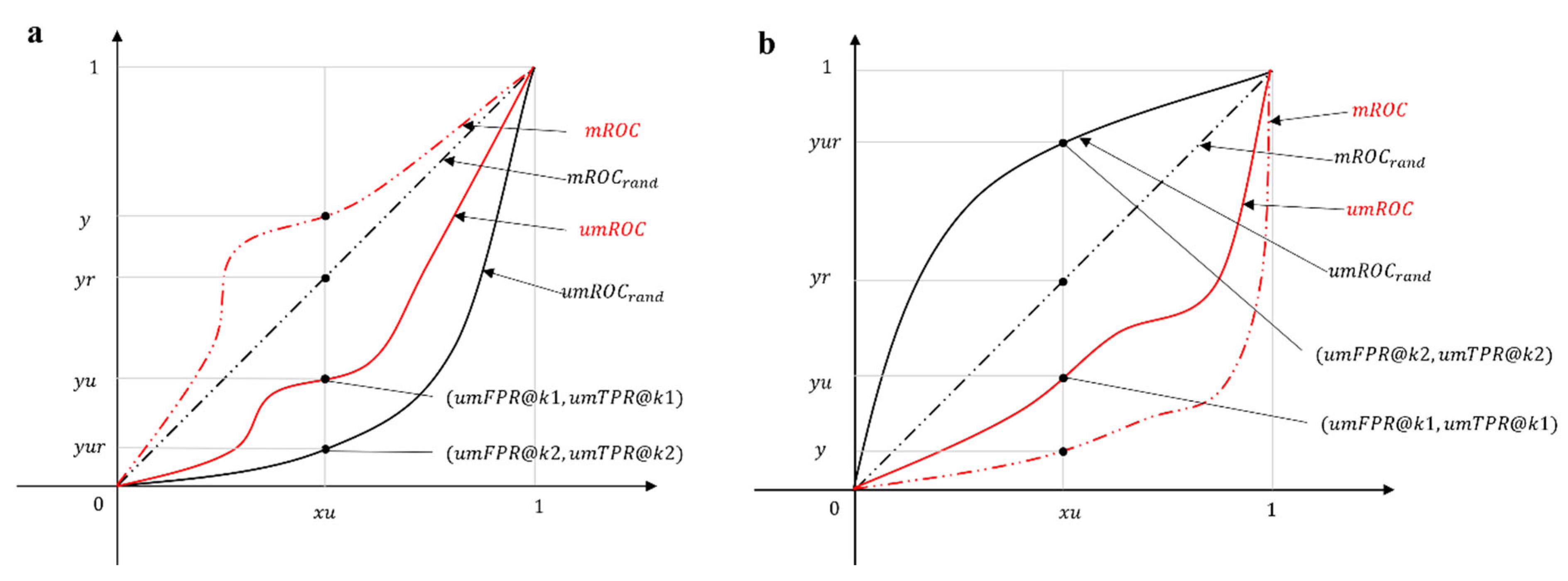
The goal of the normalization is to map these curves in a new mROC plot where the random predictor curve - as for the classical ROC curve - is the bisector of the first quadrant with coordinates x r = x u r = x u ,   y r = x r = x u and the new coordinates of the predictor are x = m F P R @ k = x u , y = m T P R @ k . To achieve this, we consider two cases separately, as illustrated in Figure 1.
The first case is visualized in Figure 1a, where y u > y u r . The un-normalized mROC curve of the actual predictor lies below the corresponding curve of the random predictor. In order to implement this mapping to the new coordinates, we perform a rescaling such that:
y y r 1 y r = y u y u r 1 y u r
The rescaling preserves the ratio of the y-axis coordinates of the two predictors with respect to the upper bound ( y = 1 ), ensuring that y r < y   1 always holds. The second case, where y u < y u r , as visualized in Figure 1b, requires a different rescaling such that:
y y r y r = y u y u r y u r
Similarly, the rescaling preserves the ratio of the y-axis coordinates of the two predictors with respect to the lower bound ( y = 0 ), ensuring that 0 y < y r always holds. Finally, by considering both cases, we arrive to the unified formula
y y r H y u y u r y r = y u y u r H y u y u r y u r
in which H is the Heaviside step function. This implies that, since y r = x r = x u :
y = ( x u H y u y u r ) ( y u H y u y u r ) y u r H y u y u r + H y u y u r
And, by substituting all the terms with their actual values, we obtain the final formula:
m T P R @ k = ( log 1 + N 1 + F P @ k 1 h ) ( log 1 + P 1 + T P @ k 1 h ) log 1 + P 1 + F P @ k 1 P / N h + h h = H ( log 1 + P 1 + T P @ k 1 1 + F P @ k 1 P / N )
The normalization is only applied to the y-axis, so that m F P R @ k = u m F P R @ k .
From Unbalanced to Balanced: A Generalized ROC (gROC) and AUC-gROC
Although the link prediction problem, like many other early retrieval problems, is often characterized by extremely unbalanced classes within the dataset, a border range of early retrieval problems encompass all possible proportions of positive and negative samples.
From the previous analysis, we know that mROC applies the same logarithm transformation on the both axes, regardless of the ratio of P and N. It defaults to the presumption that P N , such that the top-most region of the rankings is attached with more importance, while the other parts, such as the middle and bottom, are considered less relevant. This behavior is not desired for a meticulous control of the evaluation in face of less unbalanced or balanced datasets. Thus, we propose to use the mROC for extremely unbalanced dataset with few positives, while switching back to the standard ROC for balanced and inversely unbalanced cases. To allow for the automatic transition from unbalanced to balanced scenario, we proposed the generalized ROC (gROC) as follows:
g T P R @ k = 1 min 1 , P N m T P R @ k + min 1 , P N T P R @ k g F P R @ k = 1 min 1 , P N m F P R @ k + min 1 , P N F P R @ k
Indeed, gROC is a proportional mixing of mROC and ROC, such that when P N it is equal to mROC and when P N it is equal to ROC. One crucial merit of this adjustment is that the curve of a random predictor is again the bisector of the first quadrant, and the AUC-gROC of the random predictor remains at 0.5.
We claim that gROC is a class-proportion-aware metric that is apt for evaluating all types of classification and early retrieval problems, including link prediction. In the following sections, we will provide more computational evidence to demonstrate the adaptability of gROC.

Computational Experiments to Assess the Validity of AUC-gROC and AUC-mROC

As we briefly sketched in the introduction, in 2007 Truchon and Bayly [13] proposed a ‘quintessential’ argument about the inadequateness of AUC-ROC measure for evaluation of early recognition problems. They hypothesized three basic cases in which, regardless of their fundamental differences, the AUC-ROC is equal to 1/2. The first is that half of the items are retrieved at the very beginning of the rank-ordered list and the other half at the end; the second is that the items are randomly distributed all across the ranks; and the third is that all of the items are retrieved in the middle of the list. Truchon and Bayly noted that, in terms of the ‘early recognition’, the first case is clearly better than second one, which is also significantly better than the third one.
We analysed the results of a large-scale experimental study [18,19] on link prediction, which reports AUC-ROC and AUC-PR evaluations of two landmark link prediction methods - Cannistraci-Hebb adaptive network automata (CHA) and stochastic block model (SBM) - tested over 5500 simulations (550 networks x 10 repetitions). One of the interesting finding is that in 31% cases CHA has higher AUC-PR and SBM has higher AUC-ROC. In our opinion, this incongruency represents a new crucial scenario to investigate for improving our understanding about the inadequateness of AUC-ROC in evaluation of early recognition.
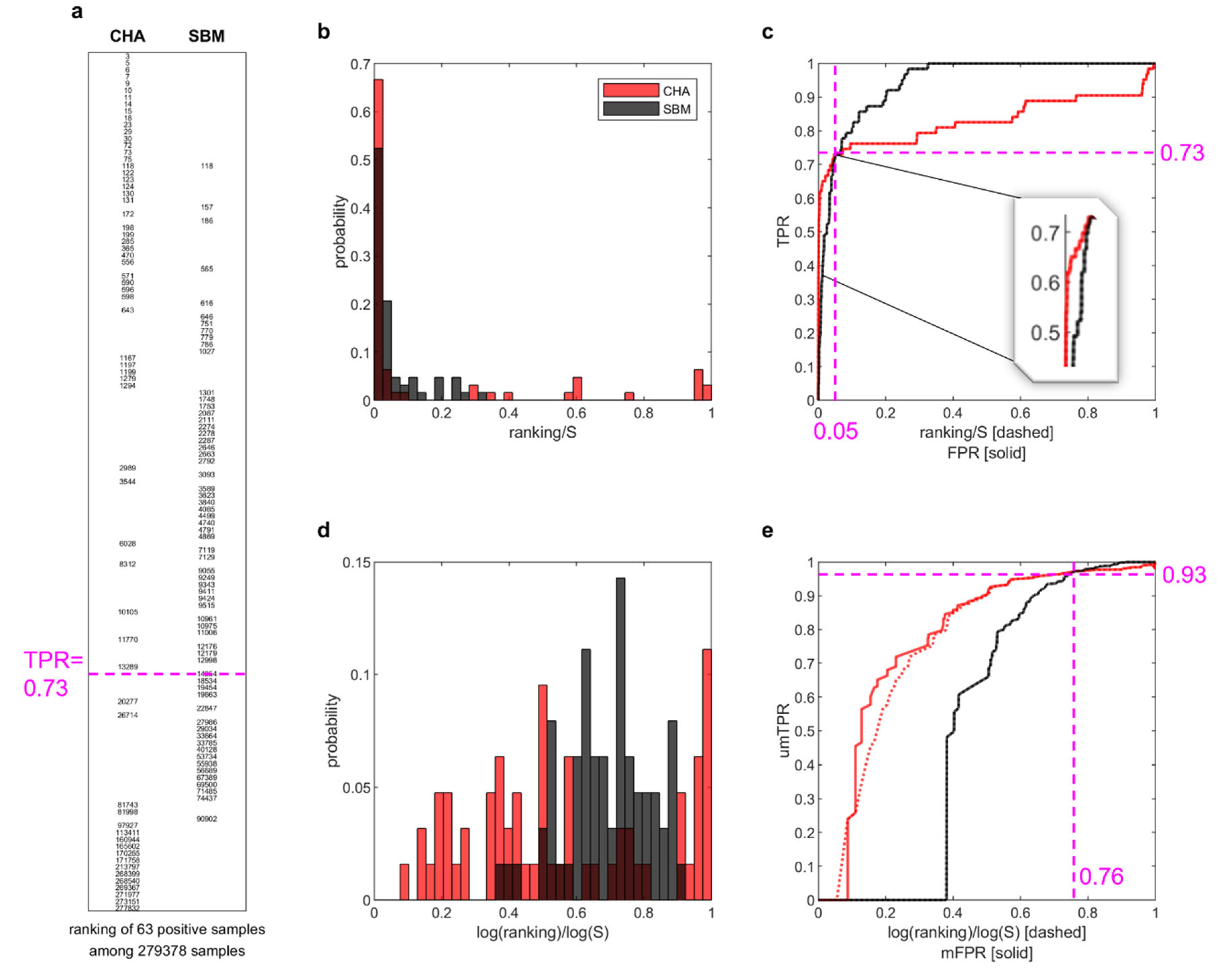
To this aim, (Figure 2 reports a paradigmatic example to investigate the AUC-ROC problem in this novel scenario. Specifically, Figure 2a displays, for both CHA and SBM, a table with the ranking positions of the 63 positive samples (i.e. the links removed in one of the tested simulations) in the ranking of 279378 non-observed links. For the first 46/63 positive samples retrieved both by CHA and SBM (i.e. up to recall 0.73, see items above magenta dashed line in Figure 2a), the ranks assigned by CHA are overall much lower than the ones assigned by SBM. Instead, the last 17/63 retrieved positive samples are better ranked by SBM (see items below the magenta dashed line in Figure 2a). Looking at this table, it is visually evident that CHA is performing better than SBM at top-ranking relevant links. This emerges, although not patently, also in Figure 2b that reports the probability of an item to occur at the different levels (ratios) of the ranking. Indeed, in this plot CHA achieves probability close to 0.7 to rank items at the very beginning, whereas SBM achieves probability slightly above 0.5. Nevertheless, the same plot might be visually misleading because the top-ranking zone is compressed very close to the y-axis and a matching with the information reported in the table of Figure 2a is not visually evident. This issue is solved in Figure 2d where the proposed adaptive logarithmic magnification of the x-axis is applied. Indeed, Figure 2d is matching the same visual information of Figure 2a, and the supremacy of CHA on SBM in top-ranking relevant links is evident.
Figure 2c displays the ROC plot associated to this example and here also, as for Figure 2a, the relevant early retrieval information is visually hidden because it is compressed very close to the y-axis. However, the fact that CHA is better then SBM in early retrieval is emerging, although not patently, also in ROC plot of Figure 2c. Indeed, if we give a closer look at the area before the crossing point (the point in which the ROCs of CHA and SBM cross each other), we can notice that (see inset in Figure 2c) the ROC of CHA clearly dominates the one of SBM. This means that in the ROC plot there is a clear early retrieval information about the fact that CHA is able to top-rank relevant links better than SBM with a 0.73 sensitivity (also termed: recall or true positive rate) and with a false positive rate of 0.05, which is low with respect to the sensitivity achieved. Practically CHA is better than SBM for the top ~15000 links of the ranking, which is the most relevant part at the application level, but this relevant part is constrained within a very small area, because the top 15000 links are only ~5% of the whole ranking (and correspond to FPR ~0.05), and ROC is giving similar importance to the entire ranking. In conclusion SBM gets a higher AUC-ROC because it performs better in the zone of the ranking that is less relevant from the application point of view. This information is not visually conveyed in the ROC plot that is misleading when we refer to the area under the curve (AUC-ROC). Indeed, the number of positive links (P = 63) is small in comparison to the non-observed ones (N = 279378 - 63), therefore the AUC-ROC ‘tells’ us more about the most abundant items that are the N, and visually neglects (confining in a small early area, see inset in Figure 2c) the information on the positive items that are in reality the one to which we are interested. Consequently, if used to evaluate early retrieval, in this scenario the AUC-ROC provides the misleading information that the performance of CHA (AUC-ROC = 0.83) is worse than SBM (AUC-ROC = 0.94).
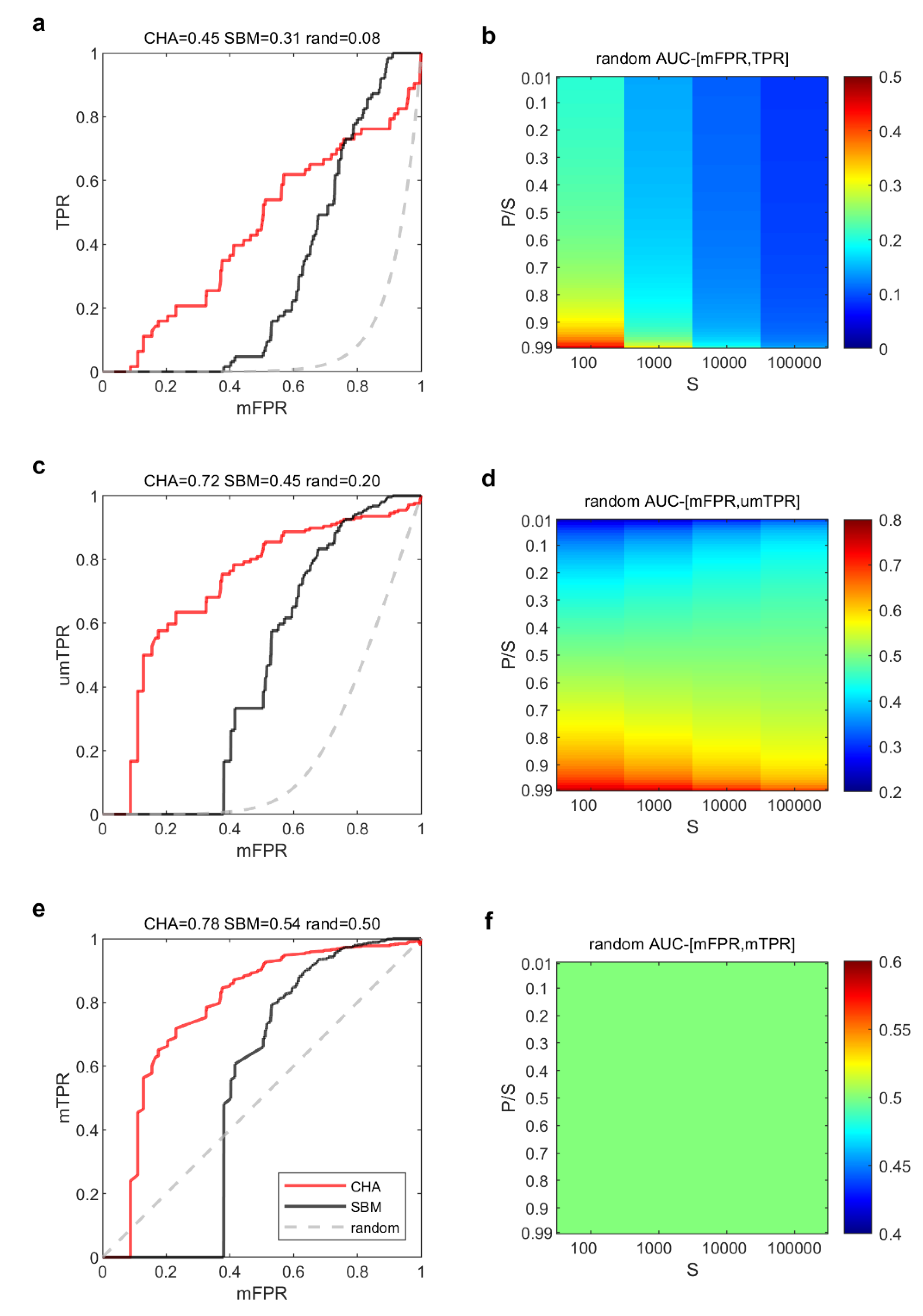
Figure 2e shows that, by applying the log adaptive magnification (proposed in this study) to both axes of the ROC plot, we can adjust the ROC plot in a way that is matching the same visual information of Figure 2a, and the supremacy of CHA on SBM in top-ranking relevant links is evident. Indeed, now the crossing point is moved to umTPR = 0.93 and mFPR = 0.76, and the merit of this adjustment is the adaptive mechanism that automatically tunes the logarithm function with respect to the number of items considered on the respective axis. However, this adjustment does not guarantee that the random predictor is always associated to a ROC that is the bisector of the first quadrant ( y = x ) and whose AUC-ROC is 0.5. This is a fundamental feature of the ROC theory and, in this study, we achieve two main findings. The first is that the log adaptive magnification of the ROC x-axis only (Figure 3a) is not enough to ensure that the AUC-ROC of the random predictor behaves symmetrically when the ration of P/N is varying, and the number of samples is growing (Figure 3b). Therefore, the log adaptive magnification of both the ROC axes is necessary (Figure 3c) in order to guarantee that this symmetry is obtained (Figure 3d). The second achievement is a consequence of the first finding, indeed once we fixed the issue of being able to analytically (see the previous section for the mathematical formula) compute the performance of the random predictor in our magnified ROC plot, now the last obstacle is to design a mathematical normalization that adjust the magnified ROC plot in a way that the random predictor has always AUC-mROC = 0.5. In the previous section we derived a mathematical theory to design this normalization. Consequently, in Figure 3e we show that the result of this normalization is able to effectively achieve our aim to provide a magnified ROC plot that respects the basic ROC theory according to which the random predictor has a mROC that follows the bisector of the first quadrant and the AUC-mROC = 0.5. Meanwhile, the magnified ROC plot in Figure3e is able to match the same visual information of Figure 2a, and the supremacy of CHA on SBM in top-ranking relevant links is explained also in terms of AUC-mROC. Indeed, the AUC-mROC provides the appropriate information that the performance of CHA (AUC-mROC = 0.78) is better than SBM (AUC-mROC = 0.54).
In all these scenarios we compared the evaluations of AUC-ROC with AUC-mROC, AUC-gROC and other baseline early retrieval evaluation measures that we commented in the introduction: precision, AUC-precision, AUC-PR, NDCG. Furthermore, we included in the comparison also the MCC as sanity check that AUC-ROC evaluation is misleading. MCC is a binary classification rate that generates a high score only if the binary predictor is able to correctly predict most of positive data instances and most of negative data instances [25,26]. Differently from AUC-ROC, MCC provides a fair estimate of the predictor performance in class unbalanced datasets such as the one in link prediction problem. However, differently from the other early retrieval evaluation measures, MCC does not attribute more importance to the positive class and it fairly and balanced considers the position in the ranking of positive and negative (in our case nonobserved links) instances. In Figure 4, on the left side, each plot reports the probability (both for CHA and SBM separately) of a positive link to occur at the different levels (ratios) of the ranking, the x-axis is transformed according to the proposed adaptive logarithm magnification function. On the right, each plot reports the performance of CHA and SBM according to the different evaluation measures.
The first scenario is the one commented till now, indeed Figure 4a coincides with the Figure 2d. We already commented above this result explaining that the AUC-ROC provides a misleading evaluation of the early retrieval performance of CHA with respect to SBM (indicating that SBM is better than CHA) because of two reasons. Firstly, in an unbalanced scenario, it gives more importance to the most abundant class that in this case is not the one of interest for the evaluation of the prediction. Secondly, according to its definition the mistakes at the bottom ranking are equally relevant as the correct predictions at the top ranking, which is not matching the purpose of link prediction in real applications. Looking at the full ranking, CHA ranks most of the positives (> 60% positives) in the top 2%, while SBM < 40% positives. In particular, with a zoom in the top 1%, CHA ranks around 16% positives in the top 0.02%, while SBM only 0.8% positives. Therefore, the performance of CHA is remarkably better than SBM at top-ranking positive links. If we look at the bottom-50% ranking, we can notice that CHA positions around 12% positives in the second half of the ranking, while SBM only 0.1%. From an application perspective, having more positives in the top-ranking at the expense of more mistakes in the bottom ranking, is much more valuable than having few positives both in the top and bottom ranking, since often for practical usage only a small fraction of the top predictions is considered, while the bottom predictions are rarely assessed. Therefore, in this scenario we would assess that CHA provides better link recommendations than SBM. This is now confirmed by the fact that in Figure 4b both AUC-mROC and all the other early retrieval measures agrees that CHA outperforms SBM in link prediction. Most importantly, even MCC - that is designed as AUC-ROC to be a binary classification rate and not an early retrieval measure - disagrees with AUC-ROC and clearly agree with the other early retrieval measures, offering an incontrovertible evidence that AUC-ROC is unreliable for evaluation of this link prediction scenario. MCC, as AUC-ROC, neglects the early retrieval nature of the problem but differently from AUC-ROC is able to adjust for the class unbalance.
The second scenario is commented in Figure 4c. CHA ranks almost all the positives (99%) in the top 1%. SBM ranks 50% of the positives in the top 1%, with 95% of the positives within the top 10% and only few positives in the bottom ranking. In this scenario, we would argue that the competition between CHA and SBM for link recommendation has a clear winner in CHA. However, looking at the value of the performance measures in Figure 3d, we can notice that AUC-ROC does not highlight the difference and it is very close for both methods (~1.00 vs 0.97), simply because both methods are good enough at not making many mistakes at the bottom ranking, which is however not the main goal of the application. Therefore, we believe that also in this scenario AUC-ROC provides a misleading assessment. This is confirmed by the results in Figure 4d, where all the other measures including AUC-mROC and MCC highlight a significant performance gap in favour of CHA with respect to SBM.
The third scenario is commented in Figure 4e. CHA is better than SBM in the top ranking, and both methods are equally bad at making some mistakes at the bottom. Therefore, in a similar scenario - as already investigated by Tao Zhou in a recent study [20] – AUC-ROC agrees with all other measures (see Figure 4f) on the fact that CHA is consistently better than SBM in link prediction. In all three scenarios, the evaluation given by AUC-gROC is almost identical to that given by AUC-mROC due to P N .
The above analysis showcases the aptness of mROC and AUC-mROC for unbalanced early retrieval problem, in which the objective is to retrieve a few most relevant samples among the vast majority of irrelevant ones. Moving towards a boarder range of problems, we may encounter cases where the proportion of the positive class is approximately equal to or even higher than that of the negative class. We investigate deeper into the scenarios with various class proportions to provide stronger computational evidence in support of the proposed measure.
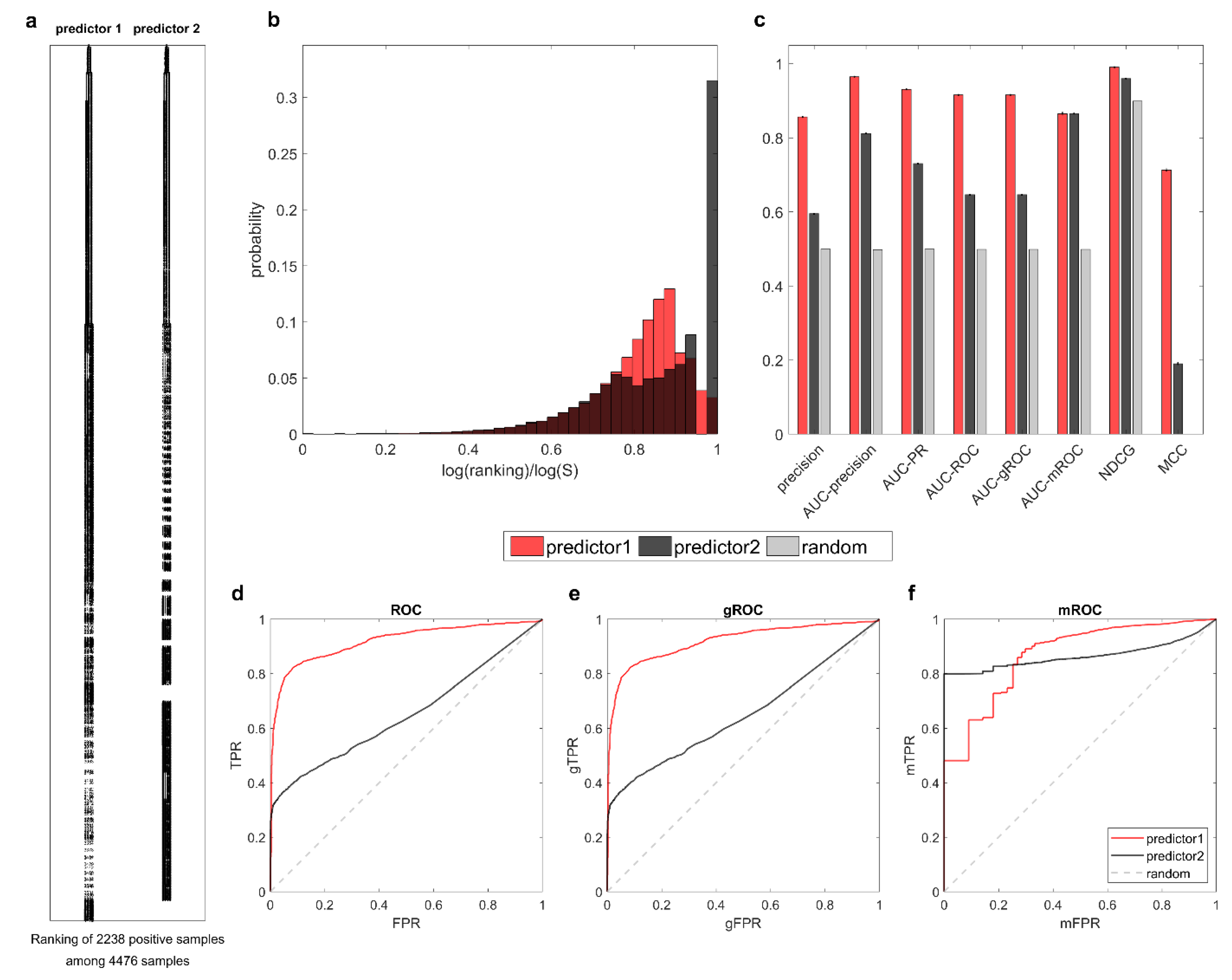
We fist consider the balanced class scenario with P N . In Figure 5, the results of predictor1 and predictor2 on the balanced class dataset are plotted, both results are generated artificially to simulate actual cases. Figure 5a displays for each predictor the ranking positions of the 2238 positive samples among the rankings of 4476 samples, and Figure 5b reports the probability distribution of the positive samples for the two predictors, in adaptive logarithm magnification scale. Both two predictors correctly rank the positive samples in the top-ranking region. However, predictor1 places more positives in the middle of the rankings than predictor2, and put a few positives at the very bottom. Its visually evident that predictor1 performs better than predictor2 in ranking the most relevant samples, and this is confirmed by all the measures in Figure 5c except for AUC-mROC. This discrepancy occurs because AUC-mROC always focuses on the top-ranking regions without considering the proportion of the positive class, leading to a misleading evaluation that suggests both predictors have similar performance. This issue is also confirmed in Figure 5f, which shows that the mTPR of predictor2 rapidly raises to 0.8 at a very low mFPR. The issue is properly resolved by gROC and AUC-gROC. As shown in Figure 5c and Figure 5e, the evaluation given by gROC and AUC-gROC is essentially the same as that given by ROC, which is desired for this scenario.
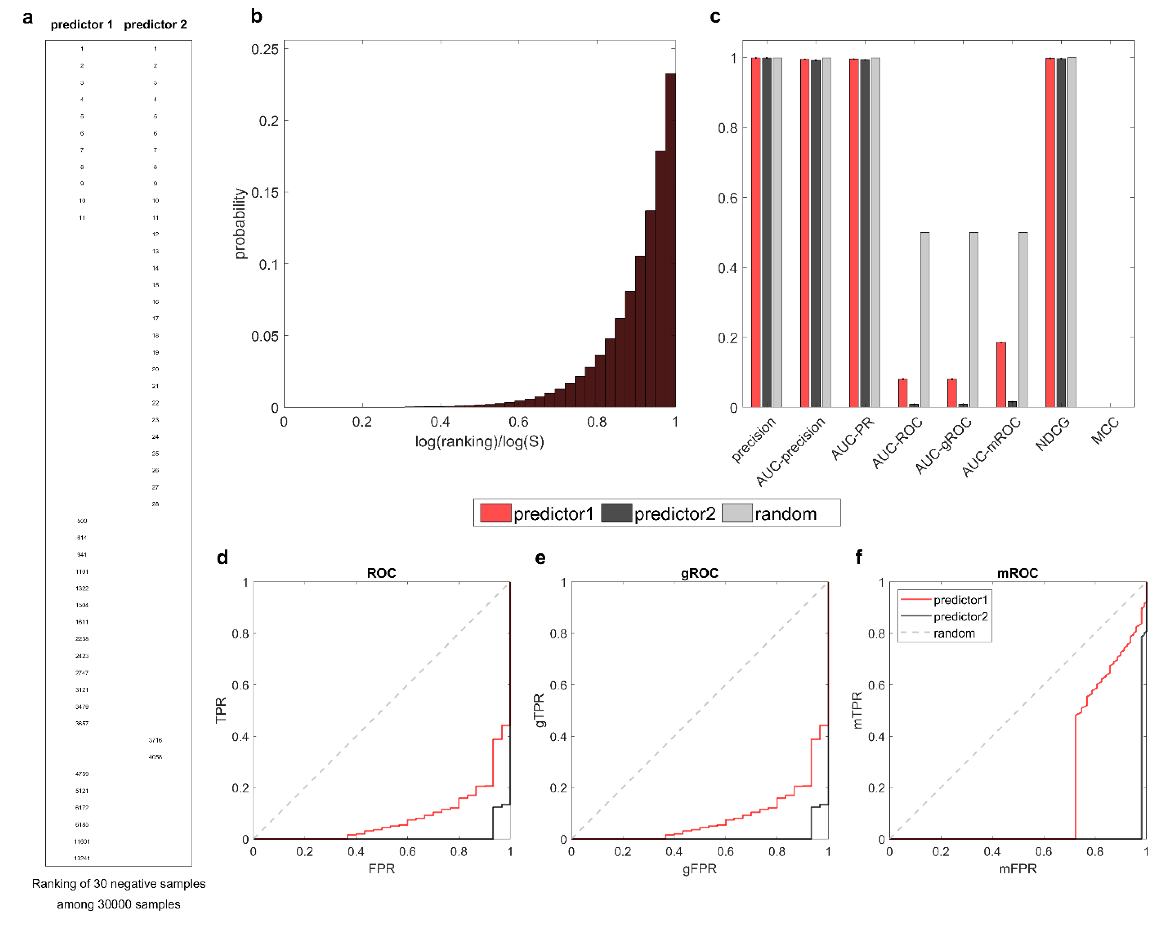
Next, we consider the inversely unbalanced scenario with P N . Again, we manipulate the results of two predictors on a dataset with 30 negative samples among 30,000 samples. In Figure 6, the two predictors mistakenly recognize negatives as positives and place them at the top of the rankings. The rankings of negative samples for the two predictors are displayed in Figure 6a. It is visually evident that predictor1 places fewer negatives at the top than predictor2, and therefore, it performs better than predictor2 under the early retrieval framework. Indeed, this conclusion is agreed upon by all three ROC-based measures: AUC-ROC, AUC-mROC, and AUC-gROC. Note that in this case, AUC-mROC exhibits a stronger discrimination capability owing to its magnification mechanism, but overall, all three measures provide a correct evaluation.
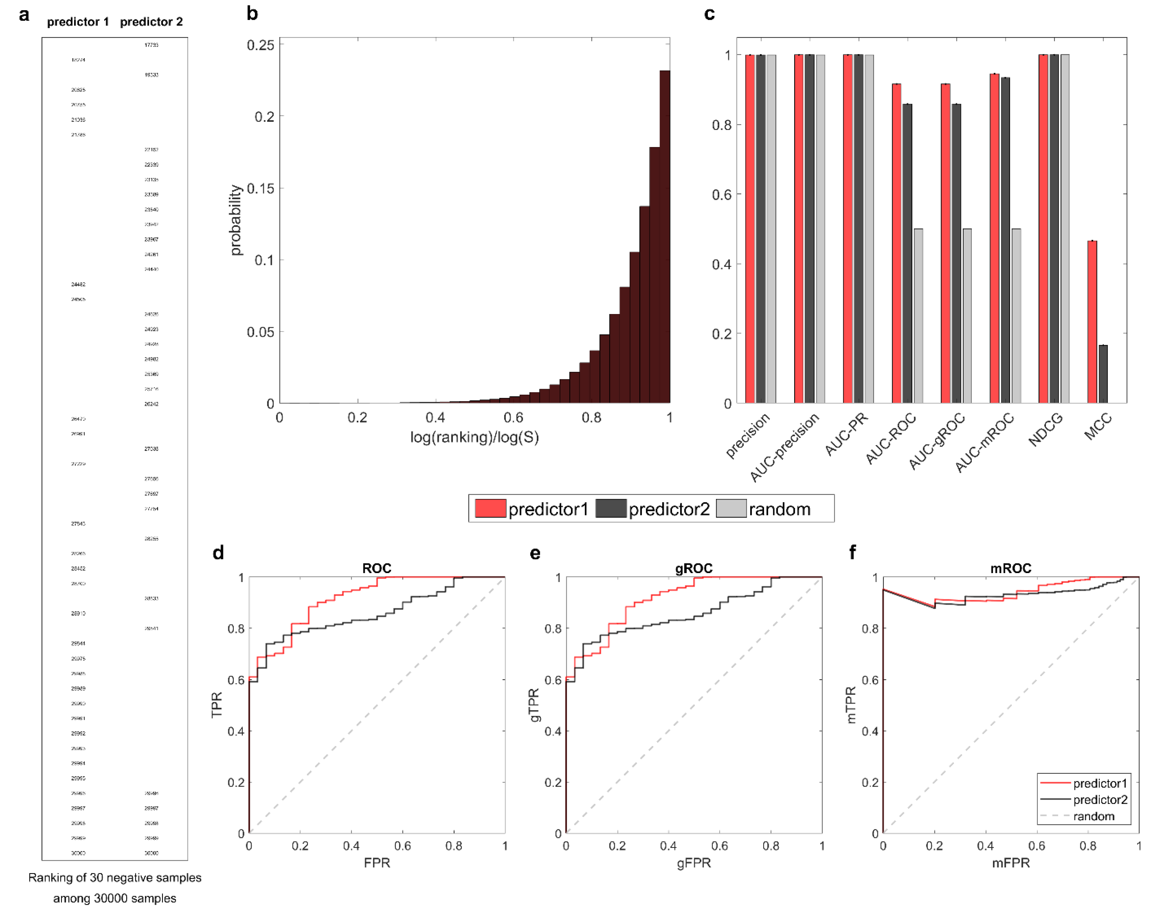
Nevertheless, for a comprehensive study, we provide in Figure 7 another example of the inversely unbalanced scenario. Analogous to the derivation in Figure 6, this time the two predictors correctly recognize most of the positives and place the few negatives at the bottom. As observed in Figure 7a, predictor1 is slightly better than predictor2 by assigning higher rankings to the negatives. Subsequently, in Figure 7c, both AUC-ROC and AUC-gROC demonstrate the superiority of predictor1, while AUC-mROC provides relatively weak differentiation. Although for the early retrieval problem, the rankings at the bottom are not as important as those at the top, this example shows that even in the worst scenario, AUC-mROC does not ignore the bottom rankings. Finally, through the computational evidence obtained in various scenarios, it is undoubtedly evident that AUC-gROC is a generalized evaluation measure suitable for early retrieval problems with arbitrary class proportions. It is elegant, parameter-free, and highly interpretable.
Table 1 emphasizes that AUC-mROC and AUC-gROC are among the measures with highest correlation to AUC-ROC, along with NDCG. This offers evidence that the AUC-mROC is an appropriate adjustment of the original AUC-ROC, and that AUC-gROC is equivalent to AUC-mROC in unbalanced scenarios. Meanwhile, AUC-mROC and AUC-gROC exhibit the highest mean correlation (Spearman correlation coefficient of 0.915) with the other measures. This evidence suggests that they are the most suitable evaluators for this task, as they demonstrate centrality within the ensemble of all evaluators. Their strong association with all the other measures makes them representative of the entire set.
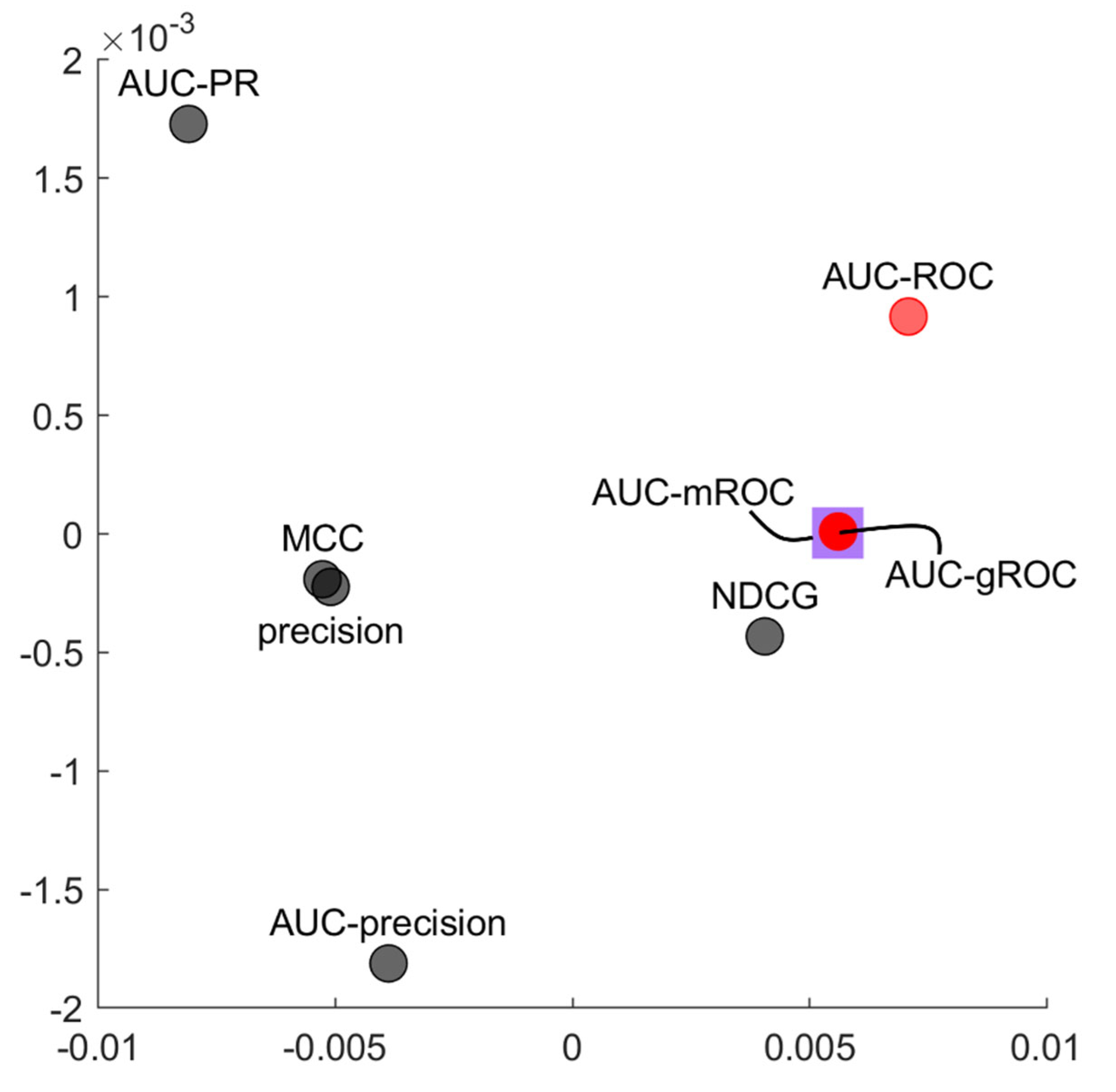
Figure 8 displays an unsupervised multidimensional analysis by means of the principal component analysis of the evaluation measures performance across all networks and link predictors (the details on the way we implemented the analysis are provided in figure legend). This knowledge representation analysis maps in a two-dimensional reduced space the relation of similarities that arise in the multidimensional space between the evaluation measures. Hence, measures that provide a similar evaluation trend (across the networks and link predictors) tend to cluster together in a similar geometrical region of the two-dimensional representation space.
AUC-ROC and AUC-gROC appears very close in the same geometrical neighbourhood and this is a further evidence (a confirmation) that, as we noted in the previous correlation analysis, the AUC-gROC is an appropriate adjustment of the original AUC-ROC. Moreover, since the evaluated networks are mostly composed of P N , AUC-gROC completely overlaps with AUC-mROC, indicating their high equivalence in this scenario.
Discussion

Differently from the previous solutions proposed in the literature - which we review in the introduction of this study - to adjust the ROC for evaluation of early retrieval problems, a remarkable achievement of gROC and AUC-gROC is that its adjustment secures, as in the standard ROC, that a random predictor follows the straight diagonal line y=x between the points (0,0) and (1,1) and, a consequence, its AUC-gROC is equal to 0.5. This is a key feature necessary to compare the performance of link predictors, indeed one of the most employed evaluation methodologies is to report their mean performance on a set of networks that belongs to the same class, and then to compare how different link predictors behave across different classes of networks. For instance, Zhou et al. [35] or Muscoloni and Cannistraci [1,18,19] showed that understanding why some link predictors perform better on a class of networks, and other link predictors excel on other classes of networks, is crucial to infer the type of rules and mechanisms that are behind the connectivity formation in diverse complex connected systems. Hence, the fact that a measure of performance such as the AUC-ROC when adjusted for early retrieval problems retains its stability (evaluating randomness at the same manner regardless of other factors) is a wished feature which becomes crucial in link prediction, and it is useful in any data science application. The AUC-gROC theory that we introduce in this study achieves this objective: on one side it preserves the original theoretical framework of the AUC-ROC and, on the other side, it is able to adjust the ROC evaluation for class unbalance early retrieval problems. The AUC-gROC does not require any parameters tuning and its major points of strength are the adaptive logarithm magnification, the normalization, and proportional mixing. The first does not require any tuning of parameters and adapts automatically the ROC plot to class unbalance, the second ensures that the random predictor follows always the bisector of the first quadrant, and the third allows for a generalized evaluation framework that works for any ratio of classes. These three innovations are the cardines of the theory proposed in this study and integrated together represents an effective solution to a problem that afflicted the field of data and network science for decades. We encourage future studies to test the AUC-gROC in evaluation scenarios different from link prediction and to spot possible flaws that we were not able to detect in the context of the current study. To this aim we openly release the code of the AUC-gROC at this link https://github.com/biomedical-cybernetics/AUC-mROC-And-AUC-gROC.

Methods

Link Prediction Evaluation Measures

  • balanced precision (or precision)
The balanced precision (or simply precision) is computed as the proportion of TP among the top-P ranked samples:
p r e c i s i o n = T P @ P P
This evaluation measure is called balanced precision [20] because, when the ranking threshold is equal to P, precision is equivalent to recall.
For the random predictor, the balanced precision is equal to the proportion of positive samples in the dataset:
p r e c i s i o n r a n d = P S
  • precision curve and AUC-precision
The precision curve is obtained by evaluating the precision at each k 1 , P :
p r e c i s i o n @ k = T P @ k k
The precision curve is composed of the points at coordinates ( k , p r e c i s i o n @ k ) for k 1 , P . The AUC-precision is obtained by computing the area under the precision curve (for example using the trapezoidal rule) and then dividing it by the width of the x-axis range that is P 1 , so that the AUC-precision is between 0 and 1.
For the random predictor, the precision is equal to the proportion of positive samples in the dataset at any ranking threshold k 1 , S :
p r e c i s i o n r a n d @ k = T P r a n d @ k k = P S
Therefore the precision curve of the random predictor is composed of the points at coordinates k , P S for k 1 , P , and the AUC-precision is equal to P S .
  • precision-recall (PR) curve and AUC-PR
The precision-recall (PR) curve is obtained by evaluating the precision and the recall at each k 1 , S :
p r e c i s i o n @ k = T P @ k k r e c a l l @ k = T P @ k P
The PR curve is composed of the points at coordinates ( r e c a l l @ k , p r e c i s i o n @ k ) for k 1 , S . The AUC-PR is obtained by computing the area under the PR curve (for example using the trapezoidal rule) and then dividing it by the width of the x-axis range that is 1 r e c a l l @ 1 , so that the AUC-PR is between 0 and 1.
For the random predictor, the precision and the recall at each k 1 , S are:
p r e c i s i o n r a n d @ k = T P r a n d @ k k = P S r e c a l l r a n d @ k = T P r a n d @ k P = k S
Therefore the PR curve of the random predictor is composed of the points at coordinates k S , P S for k 1 , S , and the AUC-PR is equal to P S .
  • Matthews correlation coefficient (MCC)
In this evaluation framework, the MCC is assessed by setting as ranking threshold k = P and computing T P @ P and F P @ P . Consequently, the number of true negatives (TN) is T N @ P = N F P @ P and the number of false negatives (FN) is F N @ P = F P @ P . Finally, the MCC formula is applied:
M C C = ( T P T N F P F N ) ( T P + F P ) ( T P + F N ) ( T N + F P ) ( T N + F N )
The MCC assumes values between -1 and 1, with 1 meaning perfect prediction, -1 meaning totally wrong prediction, and 0 being the performance of the random predictor.
  • Normalized Discounted Cumulative Gain (NDCG)
The Discounted Cumulative Gain (DCG) is computed as:
D C G = r = 1 S y r log 2 ( 1 + r )
where y r is the relevance of the sample at ranking position r . In the binary case y r = 1 for positive samples and y r = 0 for negative samples, therefore it is equivalent to summing up only the terms of the positive samples, each contributing for 1 log 2 ( 1 + r ) .
The Ideal DCG (IDCG) is the best possible DCG and it is equal to:
I D C G = r = 1 P 1 log 2 ( 1 + r )
The Normalized DCG is computed as:
N D C G = D C G I D C G
For the random predictor, we recall that the probability of assigning a positive sample to a certain ranking position is uniform over all ranking positions. Therefore, computing the DCG is equivalent to performing a uniform random sampling of P rankings (with replacement, since tied rankings are possible), and then summing up the terms associated to those P rankings. We can model each of the P terms as a function Y X of a discrete uniform random variable X : X 1 , S ,   P r o b X = r = 1 S ,   Y X = r = 1 log 2 ( 1 + r ) . The expected value is:
E Y X = r = 1 S P r o b ( X = r ) Y ( X = r ) = r = 1 S 1 S 1 log 2 ( 1 + r ) = 1 S r = 1 S 1 log 2 ( 1 + r )
Since the P random samplings are independent, the expected value of the sum of the P terms is equal to P times the expected value E Y X . Therefore the DCG and NDCG of the random predictor are:
D C G r a n d = P S r = 1 S 1 log 2 ( 1 + r ) N D C G r a n d = D C G r a n d I D C G

Link Prediction Methods

Cannistraci-Hebb Adaptive (CHA)

The Cannistraci-Hebb (CH) theory has been introduced as a revision of the local-community-paradigm (LCP) theory and it has been formalized within the framework of network automata [1,4,8], [14], [15,36,37]. While the LCP paradigm emphasized the importance to complement the information related to the common neighbours with the interactions between them (internal local-community-links), the CH rule is based on the local isolation of the common neighbours by minimizing their interactions external to the local community (external local-community-links). In particular, Cannistraci-Hebb (CH) network automata on paths of length n are all the network automata models that explicitly consider the minimization of the external local-community-links within a local community characterized by paths of length n [1]. The CH adaptive (CHA) network automaton incorporates multiple deterministic models of self-organization and automatically chooses the rule that better explains the patterns of connectivity in the network under investigation. As suggested in the original study [1], we considered the following CH models within the CHA network automaton: CH2-L2, CH3-L2, CH2-L3, CH3-L3. In addition, each of the four CH models applied the associated CH-SPcorr score for sub-ranking [1], in order to internally sub-rank all the node pairs characterized by the same CH score, reducing the ranking uncertainty of node pairs that are tied-ranked.

Stochastic Block Model (SBM)

The general idea of stochastic block model (SBM) is that the nodes are partitioned into B blocks and a B x B matrix specifies the probabilities of links existing between nodes of each block. SBM provides a general framework for statistical analysis and inference in networks, in particular for community detection and link prediction [38]. The concept of degree-corrected (DC) SBM has been introduced for community detection tasks [3] and for prediction of spurious and missing links [39], in order to keep into account the variations in node degree typically observed in real networks. We considered the implementation available in Graph-tool (http://graph-tool.skewed.de/), that adopts an optimized Monte Carlo Markov Chain (MCMC) to sample the space of the possible partitions [38]. In general the predictive performance is higher when averaging over collections of partitions than when considering only the single most plausible partition, since this can lead to overfitting [40]. Therefore, for a given network we sampled P partitions, for each partition we obtained the likelihood scores related to the non-observed links, and then considered the average likelihood scores as the link prediction result. We set P = 100 for networks with N ≤ 100, P = 50 for 100 < N ≤ 1000, P = 10 for N > 1000.
Dataset: The dataset consists of the 550 real-world networks adopted by Ghasemian et al.41. All networks are analysed as undirected, unweighted, without self-loops and only using the largest connected component. The 3 specific networks analysed in Figure 4 have the following number of nodes N, edges E, and label in the original dataset:
-network#1, N=749, E=811, 296_Norwegian_Board_of_Directors_net2mode_2006-11-01.
-network#2, N=833, E=2632, 206_Norwegian_Board_of_Directors_net1mode_2008-08-01.
-network#3, N=194, E=774, 431_5936021067ec90f1500d6597.
Hardware and software: MATLAB code has been used for CHA link prediction and evaluation. Python code has been used for SBM link prediction. The computation was executed on a Lenovo Thinkstation P920 with 1TB RAM and 2x Intel(R) Xeon(R) Gold 6242 CPU @ 2.80GHz (2x 32 cores).
Data and code availability: The dataset of 550 networks and the code for link prediction simulations related to the methods CHA and SBM are publicly available at the GitHub repository associated to the study of Muscoloni and Cannistraci [18,19]: https://github.com/biomedical-cybernetics/stealing_fire_or_stacking_knowledge_to_model_link_prediction. The MATLAB code of the AUC-gROC is publicly available at: https://github.com/biomedical-cybernetics/AUC-mROC-And-AUC-gROC.

Competing interests

The authors declare no competing financial interests.

Author Contributions

CVC conceived the idea of the AUC-mROC and AUC-gROC and drafted the formula. CVC, AM and JC contributed to the final mathematical formulations. CVC, AM and JC contributed to design the computational experiments and figures. IA generated the data for Figure 5 on evaluation of two predictors in a balanced dataset. YW contributed to design the experiments from Figure 5,Figure 6,Figure 7. CVC, AM and JC analyzed and interpreted the results. CVC wrote the main text with the help of AM and JC, and all the authors revised it. AM wrote the methods section and CVC revised it. CVC planned, directed and supervised the study.

Funding

Work in the CVC’s Center for Complex Network Intelligence was supported by the Zhou Yahui Chair professorship of Tsinghua University, the starting funding of the Tsinghua Laboratory of Brain and Intelligence, and the National High-level Talent Program of the Ministry of Science and Technology of China.

Acknowledgments

We thank YuanYuan Song, Yining Xin, Yuchi Liu and Weijie Guan for the administrative support at THBI; Hao Pang for the IT support at THBI.

References

  1. Muscoloni, A., Michieli, U. & Cannistraci, C. V. Adaptive Network Automata Modelling of Complex Networks. Preprints (2020). [CrossRef]
  2. Lü, L., Pan, L., Zhou, T., Zhang, Y.-C. & Stanley, H. E. Toward link predictability of complex networks. Proc. Natl. Acad. Sci. 112, 2325–2330 (2015).
  3. Karrer, B. & Newman, M. E. J. Stochastic blockmodels and community structure in networks. Phys. Rev. E - Stat. Nonlinear, Soft Matter Phys. 83, (2011).
  4. Cannistraci, C. V., Alanis-Lobato, G. & Ravasi, T. From link-prediction in brain connectomes and protein interactomes to the local-community-paradigm in complex networks. Sci. Rep. 3, 1–13 (2013).
  5. Lü, L. & Zhou, T. Link prediction in complex networks: A survey. Phys. A Stat. Mech. its Appl. 390, 1150–1170 (2011).
  6. Liben-Nowell, D. & Kleinberg, J. The link-prediction problem for social networks. J. Am. Soc. Inf. Sci. Technol. 58, 1019–1031 (2007).
  7. Kovács, I. A.; et al. Kovács, I. A. et al. Network-based prediction of protein interactions. Nat. Commun. (2019). [CrossRef]
  8. Muscoloni, A., Abdelhamid, I. & Cannistraci, C. V. Local-community network automata modelling based on length-three-paths for prediction of complex network structures in protein interactomes, food webs and more. bioRxiv (2018).
  9. Lichtnwalter, R. & Chawla, N. V. Link Prediction: Fair and Effective Evaluation. in 2012 IEEE/ACM International Conference on Advances in Social Networks Analysis and Mining 376–383 (2012). [CrossRef]
  10. Yang, Y. et al. Evaluating link prediction methods. Knowl. Inf. Syst. 45, 751–782 (2015).
  11. Clark, R. D. & Webster-Clark, D. J. Managing bias in ROC curves. J. Comput. Aided. Mol. Des. 22, 141–146 (2008).
  12. Swamidass, S. J., Azencott, C.-A., Daily, K. & Baldi, P. A CROC stronger than ROC: measuring, visualizing and optimizing early retrieval. Bioinformatics 26, 1348–1356 (2010).
  13. Truchon, J.-F. & Bayly, C. I. Evaluating virtual screening methods: good and bad metrics for the ‘early recognition’ problem. J. Chem. Inf. Model. 47, 488–508 (2007).
  14. Daminelli, S., Thomas, J. M., Durán, C. & Cannistraci, C. V. Common neighbours and the local-community-paradigm for topological link prediction in bipartite networks. New J. Phys. 17, 113037 (2015).
  15. Durán, C. et al. Pioneering topological methods for network-based drug–target prediction by exploiting a brain-network self-organization theory. Brief. Bioinform. 8, 3–62 (2017).
  16. Cannistraci, C. V., Alanis-Lobato, G. & Ravasi, T. Minimum curvilinearity to enhance topological prediction of protein interactions by network embedding. Bioinformatics 29, 199–209 (2013).
  17. Zhou, T. Progresses and challenges in link prediction. iScience 24, 103217 (2021).
  18. Muscoloni, A. & Cannistraci, C. V. Short Note on Comparing Stacking Modelling Versus Cannistraci-Hebb Adaptive Network Automata for Link Prediction in Complex Networks. Preprints (2021).
  19. Muscoloni, A. ‘Stealing fire or stacking knowledge’ by machine intelligence to model link prediction in complex networks. (submitted) (2022).
  20. Zhou, T. Discriminating abilities of threshold-free evaluation metrics in link prediction. arXiv:2205.04615, arXiv:2205.04615 (2022).
  21. Provost, F. J., Fawcett, T. & Kohavi, R. The Case against Accuracy Estimation for Comparing Induction Algorithms. in Proceedings of the Fifteenth International Conference on Machine Learning 445–453 (Morgan Kaufmann Publishers Inc., 1998).
  22. Davis, J. & Goadrich, M. The Relationship Between Precision-Recall and ROC Curves. Proc. 23rd Int. Conf. Mach. Learn. -- ICML’06 233–240 (2006). [CrossRef]
  23. Matthews, B. W. Comparison of the predicted and observed secondary structure of T4 phage lysozyme. Biochim. Biophys. Acta - Protein Struct. 405, 442–451 (1975).
  24. Yule, G. U. On the Methods of Measuring Association Between Two Attributes. J. R. Stat. Soc. 75, 579–652 (1912).
  25. Jurman, G., Riccadonna, S. & Furlanello, C. A comparison of MCC and CEN error measures in multi-class prediction. PLoS One 7, e41882 (2012).
  26. Chicco, D. Ten quick tips for machine learning in computational biology. BioData Min. 10, 35 (2017).
  27. McClish, D. K. Analyzing a portion of the ROC curve. Med. Decis. Mak. an Int. J. Soc. Med. Decis. Mak. 9, 190–195 (1989).
  28. Walter, S. D. The partial area under the summary ROC curve. Stat. Med. 24, 2025–2040 (2005).
  29. Carrington, A. M. et al. A new concordant partial AUC and partial c statistic for imbalanced data in the evaluation of machine learning algorithms. BMC Med. Inform. Decis. Mak. 20, 4 (2020).
  30. McClish, D. K. Evaluation of the Accuracy of Medical Tests in a Region around the Optimal Point. Acad. Radiol. 19, 1484–1490 (2012).
  31. Jiang, Y., Metz, C. E. & Nishikawa, R. M. A receiver operating characteristic partial area index for highly sensitive diagnostic tests. Radiology 201, 745–750 (1996).
  32. Jiang, Y., Metz, C. E. & Nishikawa, R. M. A receiver operating characteristic partial area index for highly sensitive diagnostic tests. Radiology 201, 745–750 (1996). [CrossRef]
  33. Järvelin, K. & Kekäläinen, J. Cumulated Gain-Based Evaluation of IR Techniques. ACM Trans. Inf. Syst. 20, 422–446 (2002).
  34. Sheridan, R. P., Singh, S. B., Fluder, E. M. & Kearsley, S. K. Protocols for bridging the peptide to nonpeptide gap in topological similarity searches. J. Chem. Inf. Comput. Sci. 41, 1395–1406 (2001).
  35. Zhou, T., Lee, Y.-L. & Wang, G. Experimental analyses on 2-hop-based and 3-hop-based link prediction algorithms. Phys. A Stat. Mech. its Appl. 564, 125532 (2021).
  36. Cannistraci, C. V. Modelling Self-Organization in Complex Networks Via a Brain-Inspired Network Automata Theory Improves Link Reliability in Protein Interactomes. Sci. Rep. 8, 15760 (2018).
  37. Muscoloni, A. & Cannistraci, C. V. Local-ring network automata and the impact of hyperbolic geometry in complex network link-prediction. arXiv:1707.09496 [physics.soc-ph] (2017). arXiv:1707.09496 [physics.soc-ph] (2017).
  38. Peixoto, T. P. Efficient Monte Carlo and greedy heuristic for the inference of stochastic block models. Phys. Rev. E - Stat. Nonlinear, Soft Matter Phys. 89, (2014).
  39. Zhang, X., Wang, X., Zhao, C., Yi, D. & Xie, Z. Degree-corrected stochastic block models and reliability in networks. Phys. A Stat. Mech. its Appl. 393, 553–559 (2014).
  40. Vallès-Català, T., Peixoto, T. P., Sales-Pardo, M. & Guimerà, R. Consistencies and inconsistencies between model selection and link prediction in networks. Phys. Rev. E (2018). 2018. [CrossRef]
  41. Ghasemian, A., Hosseinmardi, H., Galstyan, A., Airoldi, E. M. & Clauset, A. Stacking models for nearly optimal link prediction in complex networks. Proc. Natl. Acad. Sci. U. S. A. (2020). [CrossRef]
Figure 1. The normalization principle of the magnified ROC curve. The figure demonstrates the normalization principle behind the derivation of mROC. Red coloured lines represent the curves of the actual predictor, and the black coloured lines represent the curves of the random predictor. The un-normalized magnified ROC (umROC) curves are shown as solid lines, and the curves after normalization (mROC) are represented by dashed lines. x u , y u and y correspond to the u m F P R , u m T P R and m T P R of the actual predictor, obtained at threshold k 1 . y u r and y r correspond to the u m T P R and m T P R of the random predictor, obtained at threshold k 2 . (a) The panel reports the case when y u > y u r . (b) The panel reports the case when y u < y u r .
Preprints 112817 g001
Figure 2. The rationale behind the magnified ROC curve. The figure reports the results for CHA and SBM methods in a representative link prediction simulation (10% link removal evaluation) on the network#1. (a) The panel shows the positions of the 63 positive samples (i.e. the 10% of links removed) among the ranking of 279378 samples (i.e. all the non-observed links in the network after 10% link removal). (b) The panel shows the probability distribution of the rankings of the positive samples according to the predictions of CHA and SBM, considering the rankings divided by the maximum. The probability distribution is approximated with a histogram of 40 bins equally spaced between 0 and 1. (c) The panel shows the curves [ranking/S,TPR] (dashed lines) and the curves [FPR,TPR] (solid lines) for the methods CHA (red), SBM (black). (d) The panel is analogous to panel (b), considering the rankings in adaptive logarithm magnification scale. (e) The panel shows the curves [log(ranking)/log(S),umTPR] (dashed lines) and the curves [mFPR,umTPR] (solid lines) for the methods CHA (red), SBM (black). Note that in highly imbalanced datasets, the ranking proportions (dashed line) are approximately equal to the FPR (solid line), so we can report both on the x-axis and the associated ROCs have a similar trend.
Preprints 112817 g002
Figure 3. Magnification and normalization of TPR. (a,c,e) The panels report the results in a representative link prediction simulation (10% link removal evaluation) on the network#1. They show, respectively, the curves (a) [mFPR,TPR], (c) [mFPR,umTPR] and (e) [mFPR, mTPR], for the methods CHA (red solid), SBM (black solid) and random predictor (grey dashed). The corresponding AUC performances are reported on top of each subplot. (b) For each sample size S = [100, 1000, 10000, 100000], for each proportion of positives P/S from 0.01 to 0.99 at steps of 0.01, the heatmap reports the AUC of the curve [mFPR,TPR] for the random predictor. (d) The heatmap is analogous to (b) for the AUC of the curve [mFPR,umTPR] for the random predictor. (f) The heatmap reports the AUC of the curve [mFPR, mTPR] for the random predictor.At this stage of the study we deepen our investigation. Among all 550 real networks recently analysed in the large-scale experimental link-prediction paper of Muscoloni and Cannistraci [18,19], in Figure 4 we selected three representative scenarios: 1) inverse trend of AUC-PR and AUC-ROC (which is the same scenario discussed in the previous figures); 2) large AUC-PR difference and similar AUC-ROC; 3) similar trend of AUC-PR and AUC-ROC (which is similar to the scenario considered by Tao Zhou in one of his recent studies [20]). In order to allow replication of these results, the networks identities in which these scenarios occur are reported in the Dataset sub-section of the Method section.
Preprints 112817 g003
Figure 4. CHA and SBM link prediction results: three case studies. The figure reports the link prediction results for CHA and SBM methods on three case studies: network#1, network#2 and network#3 (see Methods for the information on the network identity). (a,c,e) The panels show the probability distribution of the rankings of the positive samples according to the predictions of CHA and SBM, considering the rankings in adaptive logarithm magnified scale. Each probability distribution is approximated with a histogram of 40 bins equally spaced between 0 and 1. To improve the statistical robustness of the distribution, the histograms are computed on rankings combined from 10 repetitions of the link prediction evaluation. (b,d,f) The panels show the mean and standard error of several evaluation measures over 10 repetitions of the link prediction evaluation, for CHA, SBM and random predictor.
Preprints 112817 g004
Figure 5. Evaluation of two predictors on a balanced dataset. The figure reports the results of two predictors generated artificially on a balanced dataset with P N (a) The panel shows the positions of the 2238 positive samples among the rankings of 4476 samples. (b) The panel shows the probability distribution of the rankings of the positive samples according to the predictions of predictor1 and predictor2 in adaptive logarithm magnification scale. The probability distribution is approximated by a histogram with 40 bins spaced between 0 and 1. (c) The panel shows the values of several evaluation measures for predictor1, predictor2 and the random predictor. (d, e, f) The panels show the (d) ROC curves [FPR,TPR], (e) gROC curves [gFPR,gTPR], and (f) mROC curves [mFPR,mTPR] for predictor1 (red solid), predictor2 (black solid), and random predictor (grey dashed), respectively.
Preprints 112817 g005
Figure 6. Evaluation of two predictors on an inversely balanced dataset: negatives at the top. The figure reports the results of two predictors generated artificially on an inverse unbalanced dataset with P N The two predictors mistakenly recognize negatives as positives and place them at the top of the rankings. (a) The panel shows the positions of the 30 negative samples among the rankings of 30000 samples. (b) The panel shows the probability distribution of the rankings of the positive samples according to the predictions of predictor1 and predictor2 in adaptive logarithm magnification scale. The probability distribution is approximated by a histogram with 40 bins spaced between 0 and 1. (c) The panel shows the values of several evaluation measures for predictor1, predictor2 and the random predictor. (d, e, f) The panels show the (d) ROC curves [FPR,TPR], (e) gROC curves [gFPR,gTPR], and (f) mROC curves [mFPR,mTPR] for predictor1 (red solid), predictor2 (black solid), and random predictor (grey dashed), respectively.
Preprints 112817 g006
Figure 7. Evaluation of two predictors on an inversely balanced dataset: negatives at the bottom. The figure reports the results of two predictors generated artificially on an inverse unbalanced dataset with P N The two predictors mistakenly recognize negatives as positives and place them at the top of the rankings. (a) The panel shows the positions of the 30 negative samples among the rankings of 30000 samples. (b) The panel shows the probability distribution of the rankings of the positive samples according to the predictions of predictor1 and predictor2 in adaptive logarithm magnification scale. The probability distribution is approximated by a histogram with 40 bins spaced between 0 and 1. (c) The panel shows the values of several evaluation measures for predictor1, predictor2 and random predictor. (d, e, f) The panels show the (d) ROC curves [FPR,TPR], (e) gROC curves [gFPR,gTPR], and (f) mROC curves [mFPR,mTPR] for predictor1 (red solid), predictor2 (black solid), and random predictor (grey dashed), respectively.
Preprints 112817 g007
Figure 8. PCA of evaluation measures. The 10% link removal evaluation has been run for CHA and SBM on all the 550 networks of the dataset (10 repetitions), obtaining for each of the 8 evaluation measures a total of 2x550x10=11000 values. The figure shows the first two principal components of the 8 evaluation measures obtained performing PCA on the 8x11000 matrix (each row of the matrix has been normalized by the sum). All the evaluation measures are shown as black circles except for AUC-mROC (purple square), AUC-ROC, and AUC-gROC (red circle), in order to highlight their proximity in the PC space.
Preprints 112817 g008
Table 1. Correlation of evaluation measures. The 10% link removal evaluation has been run for CHA and SBM on all the 550 networks of the dataset (10 repetitions), obtaining for each of the 8 evaluation measures a total of 2x550x10=11000 values. The table reports, for each pair of evaluation measures, the Spearman correlation coefficient computed between the two respective vectors of 11000 values. At the bottom, the table shows the mean Spearman correlation between each evaluation measure and the others. The measures with the highest mean correlation to all measures are highlighted in bold.
precision AUC-precision AUC-PR AUC-ROC AUC-mROC AUC-gROC NDCG MCC
precision 0.98 0.95 0.65 0.94 0.94 0.94 0.99
AUC-precision 0.98 0.94 0.63 0.96 0.96 0.95 0.97
AUC-PR 0.95 0.94 0.66 0.93 0.93 0.93 0.91
AUC-ROC 0.65 0.63 0.66 0.70 0.70 0.71 0.66
AUC-mROC 0.94 0.96 0.93 0.70 1.00 0.94 0.93
AUC-gROC 0.94 0.96 0.93 0.70 1.00 0.94 0.93
NDCG 0.94 0.95 0.93 0.71 0.94 0.94 0.93
MCC 0.99 0.97 0.91 0.66 0.93 0.93 0.93
mean 0.912 0.914 0.893 0.673 0.915 0.915 0.906 0.903
Disclaimer/Publisher’s Note: The statements, opinions and data contained in all publications are solely those of the individual author(s) and contributor(s) and not of MDPI and/or the editor(s). MDPI and/or the editor(s) disclaim responsibility for any injury to people or property resulting from any ideas, methods, instructions or products referred to in the content.
Copyright: This open access article is published under a Creative Commons CC BY 4.0 license, which permit the free download, distribution, and reuse, provided that the author and preprint are cited in any reuse.
Prerpints.org logo

Preprints.org is a free preprint server supported by MDPI in Basel, Switzerland.

Subscribe

© 2024 MDPI (Basel, Switzerland) unless otherwise stated