The Principle "Like Begets Like" in Molecular and Algebraic-Matrix Genetics

Preprint

Article

The Principle "Like Begets Like" in Molecular and Algebraic-Matrix Genetics

Altmetrics

Downloads

366

Views

171

Comments

Sergey Petoukhov^*

This version is not peer-reviewed

Submitted:

23 May 2023

Posted:

25 May 2023

You are already at the latest version

Alerts

Abstract

This article is devoted to the results of in-depth analysis of the system of binary-oppositional structures in DNA n-plet alphabets and their algebraic-matrix representations. These results show that the molecular complementary replication of DNA strands is accompanied by the presence of an algebraic version of the principle "like begets like" in matrix representations of DNA alphabets having internal structures. This algebraic version is based on binary-oppositional structures in the genetic molecular system, which can be represented by binary numbers and corresponding matrices of DNA alphabets. The received results allow thinking that the phenomenon "like begets like" (or a complementary replication in a wide sense) is systemic in the genetic organization and is connected with algebraic features of biological organization. Correspondingly, the biological principle "like begets like" can be additionally modeled by algebraic-matrix methods and approaches. Such algebra-matrix modeling of the genetic coding system gives new ways for studying and understanding the key role of the named principle in genetic and other inherited physiological complexes. On this way, the author discovered general rules of stochastic organization of information binary sequences of genomic DNAs of eukaryotes and prokaryotes. The presented rules are connected with information dichotomies of probabilities and corresponding fractal-like trees of probabilities, which fundamentally differ from constructional dichotomies in biological bodies. The received phenomenological data and rules lead to new biological ideas.

Keywords:

Subject: Biology and Life Sciences - Biochemistry and Molecular Biology

Introduction
Symmetries and binary principles in the molecular genetic system
Complementary-replicated genetic matrices and the even-odd columns decomposition of the matrix of 64 triplets
Complementary-replicated genetic matrices and the even-odd rows decomposition of the matrix of 64 triplets
Complementary replications and the matrix of 64 triplets under its twice-complementary transformation
Genetic matrices, root-complementarity, and hyperbolic numbers
Universal algorithms for dichotomies of probabilities in hydrogen bond sequences of genomic DNAs

-

7.1. Suffix dichotomies of percentages of H-n-plets in DNA of human chromosome № 1

--

7.1.1. The rule of percentage equalities in the set of genomic H-n-plets

-

7.2. Prefix dichotomies of percentages of H-n-plets in DNA of human chromosome № 1

-

7.3. Regarding importance of hydrogen bonds and the binary-stochastic analogy between genetic and nervous systems

-

7.4. Dichotomies of percentages of H-n-plets in DNA of the plant Arabidopsis Thaliana

-

7.5. Dichotomies of percentages of H-n-plets in genomic DNA of the bacteria Bradyrhizobium japonicum
Universal algorithms for dichotomies of probabilities in purine-pyrimidine sequences of genomic DNAs

-

8.1. Suffix dichotomies of percentages of n-plets in the purine-pyrimidine sequence of DNA of human chromosome № 1

-

8.2. Percent palindromes and the rule of equality of percent values of complementary purine-pyrimidine n-plets in genomic DNAs

-

8.3. Suffix dichotomies of percentages of n-plets in the purine-pyrimidine sequence of DNA of the chromosome № 1 of the plant Arabidopsis thaliana

-

8.4. Suffix dichotomies of percentages of n-plets in the purine-pyrimidine sequence of DNA of the chromosome № 1 of the plant Arabidopsis thaliana
Universal algorithms for dichotomies of probabilities in keto-amino sequences of genomic DNAs

-

9.1. Suffix dichotomies of percentages of n-plets in the keto-amino sequence of DNA of human chromosome № 1

-

9.2. Suffix dichotomies of percentages of n-plets in the keto-amino sequence of DNA of chromosome № 1 of the plant Arabidopsis thaliana

-

9.3. Suffix dichotomies of percentages of n-plets in the keto-amino sequence of the genomic DNA of the bacteria Bradyrhizobium japonicum
Parallelism between dichotomies in inherited biological bodies and universal dichotomies of probabilities in stochastic organization of genomic DNAs
Parallelism between dichotomies in inherited biological bodies and universal dichotomies of probabilities in stochastic organization of genomic DNAs

-

11.1. The HBS-analysis of the sequence of hydrogen bonds in the gene TTN

-

11.2. The HBS-analysis of the purine-pyrimidine sequence of the gene TTN

-

11.3. The HBS-analysis of the keto-amino sequence in the gene TTN
Algebra-matrix representations of alphabetic families of probabilities of n-plets in binary DNAs sequences

-

12.1. Alphabetic matrices of H-n-plets percentages and 2ⁿ-dimensional hyperbolic numbers

-

12.2. Alphabetic matrices of H-n-plets percentages, characteristic polynomials, and algebraic geometry

-

12.3. Alphabetic matrices of H-n-plets percentages and metric tensors
Alphabetic matrices of percentages of n-plets in cases of binary sequences of purines-pyrimidines and keto-amino elements in DNAs
Quantum-information formalisms in analysis of stochastic binary sequences of DNAs

Some concluding remarks

Acknowledgments

References

1. Introduction

The DNA double helix model created by J.D. Watson and F. Crick in 1953 gave a powerful impetus to the development of genetic research. It showed the world a recursive algorithm for the complementary replication of DNA strands, which ensures the replication of the genetic information recorded on these strands. Before the complementary replication, DNA is separated in two complementary strands. Each strand of the original DNA molecule serves as a template for the production of its new complementary counterpart. This seminal work by Watson and Crick was perceived as the discovery of a key secret of life, corresponding to the ancient notion that “like begets like”. Scientists were struck by how simple and beautiful this explanation of the replication and preservation of genetic information based on the mechanism of complementarity turned out to be. It was emphasized that it is this complementarity that provides the most important properties of DNA as a carrier of hereditary information (see, for example, [Chapeville, Haenni,1974]).

The complementary replication of DNA occurs in all living organisms acting as the most essential part of biological inheritance. This is essential for cell division during the growth and repair of damaged tissues, while it also ensures that each of the new cells receives its own copy of the DNA. The cell possesses the distinctive property of division, which makes complementary replication of DNA essential. Complementary replication of DNA strands occurs at an astonishing speed rate. For example, the well-known bacteria E. coli has a speed of replication of over 1,000 bases per second [Bank, 2022].

The genetic information in DNA molecules is represented in the form of sequences of four types of nucleobases: adenine A, guanine G, cytosine C, and thymine T. Their set is often referred to as the 4-letter DNA alphabet. Along with it, other DNA alphabets exist: alphabets of 16 doublets, 64 triplets, 256 tetraplets, and other n-plets. In particular, the alphabet of 64 triplets is used in the genetic system to encode amino acids and termination signals of protein synthesis. Taking into account the existence of different alphabets of DNA n-plets turns out to be useful for revealing hidden regularities in the stochastic organization of genomic DNAs [Petoukhov, 2008, 2020, 2021a,b; Petoukhov, He, 2010]. These DNA alphabets have binary-oppositional structures, which allow representing the alphabets in a comfortable form of (2ⁿ*2ⁿ)-matrices with dispositions - inside these matrices - of all corresponding n-plets in strict arrangements on the basis of their individual molecular peculiarities [Petoukhov, 2008; Petoukhov, He, 2010].

The purpose of this article is to describe the author’s results of an in-depth analysis of the system of binary-oppositional structures in these DNA alphabets and their algebraic-matrix representations. These results show that the molecular complementary replication of DNA strands is accompanied by the presence of an algebraic version of the principle “like begets like” in the named matrix representations of DNA alphabets. This algebraic version is based on binary-oppositional structures in the genetic molecular system, which can be represented by binary numbers and corresponding matrices of DNA alphabets. The received results allow thinking that the phenomenon “like begets like” (or a complementary replication in a wide sense) is systemic in the genetic organization and is connected with algebraic features of biological organization. Correspondingly, the biological principle “like begets like” can be additionally modeled by algebraic-matrix methods and approaches. Such algebraic-matrix modeling of the genetic coding system gives new ways for studying and understanding a key role of the named principle in genetic and other inherited physiological complexes.

2. Symmetries and binary principles in the molecular genetic system

The four nucleobases of DNA are interrelated by their symmetrical peculiarities into the united molecular ensemble having the three pairs of binary-oppositional traits or indicators [Fimmel, Danielli, Strüngmann, 2013; Petoukhov, 2008; Petoukhov, He, 20010; Stambuk, 1999]:

(1): Two letters are purines (A and G), and the other two are pyrimidines (C and T). From the standpoint of these binary-oppositional traits one can denote C = T = 0, A = G = 1. From the standpoint of these traits, any of the DNA-sequences are represented by a corresponding binary sequence. For example, the sequence GCATGAAGT is represented by binary sequence 101011110;
(2): Two letters are amino-molecules (A and C) and the other two are keto-molecules (G and T). From the standpoint of these traits one can designate A = C = 0, G = T = 1. Correspondingly, the same sequence GCATGAAGT, as above, is represented by another binary sequence, 100110011;
(3): The pairs of complementary letters, A-T and C-G, are linked by 2 and 3 hydrogen bonds, respectively. From the standpoint of these traits, one can designate C = G = 0, A = T = 1. Correspondingly, the same sequence GCATGAAGT, is read as the binary sequence 001101101.

These three types of binary representations form a common logic set on the basis of logic operation of modulo-2 addition denoted by the symbol

\oplus

: modulo-2 addition of any two such binary representations of the DNA-sequence gives a sum, which is equal to the third binary representation of the same DNA-sequence: for example, 101011110

\oplus

100110011 = 001101101. One can here remind the rules of the bitwise modulo-2 addition: 0

\oplus

0 = 0; 0

\oplus

1 = 1; 1

\oplus

0 = 1; 1

\oplus

1 = 0. (The logic operation of modulo-2 addition is actively used in computer informatics and quantum informatics).

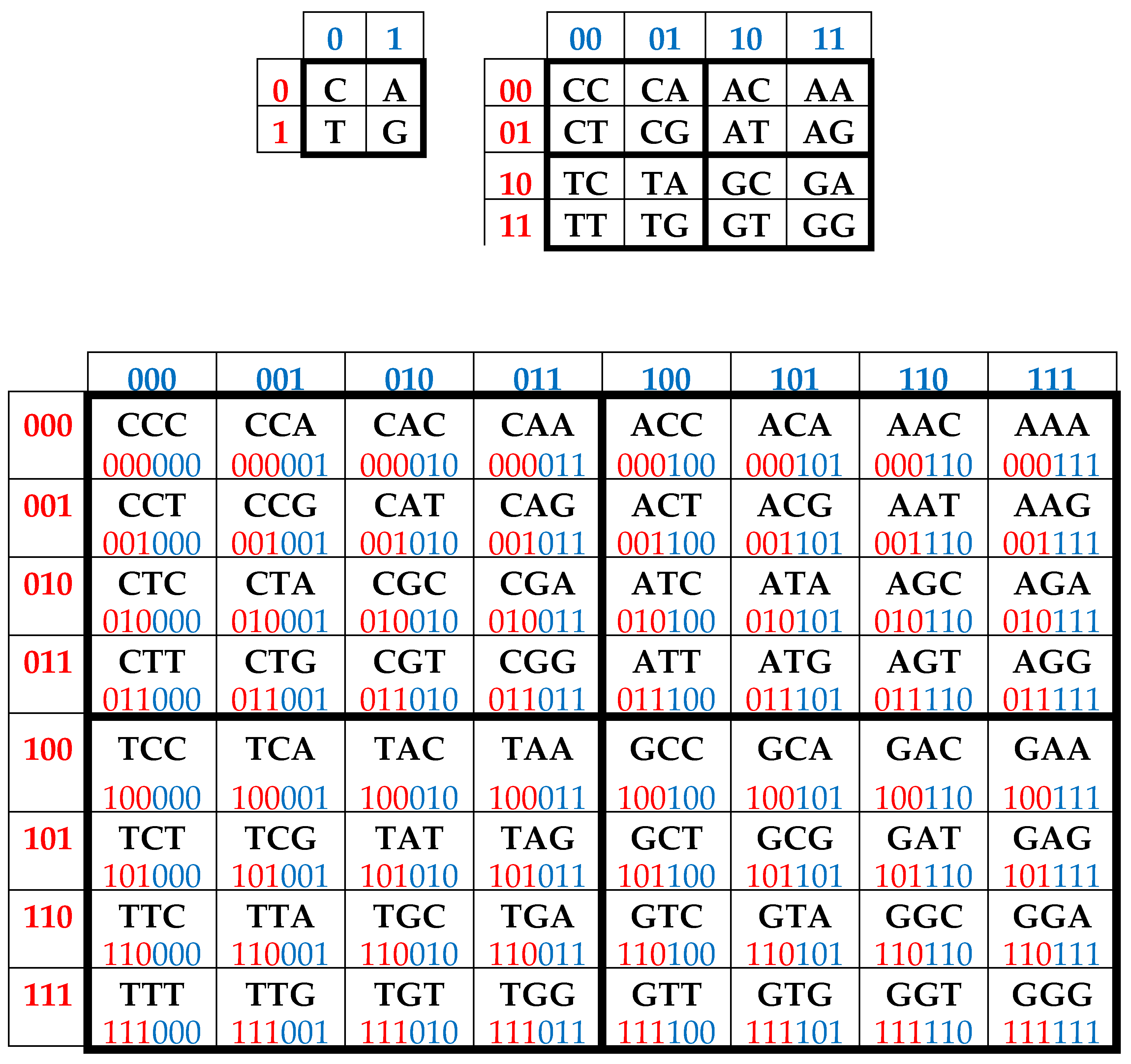
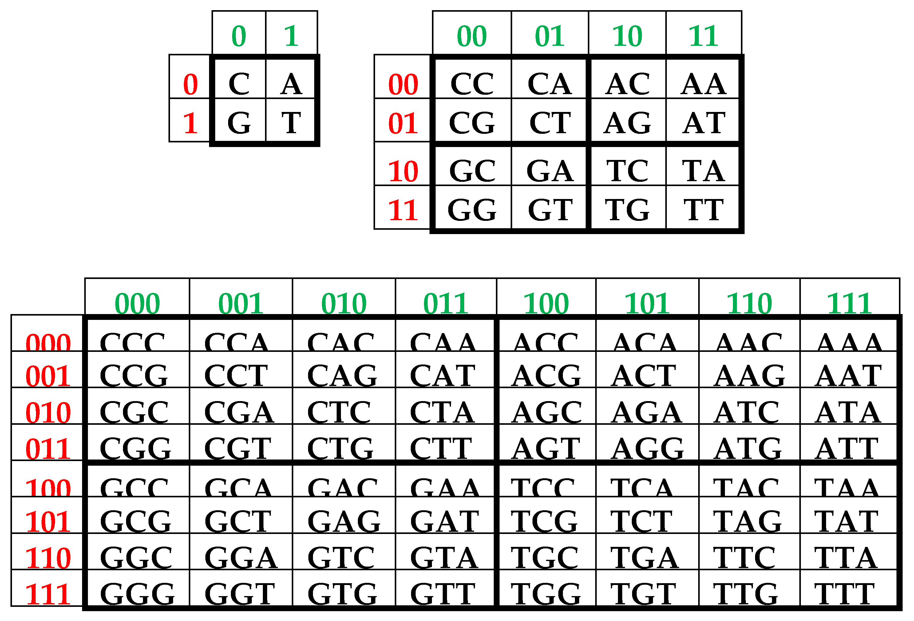
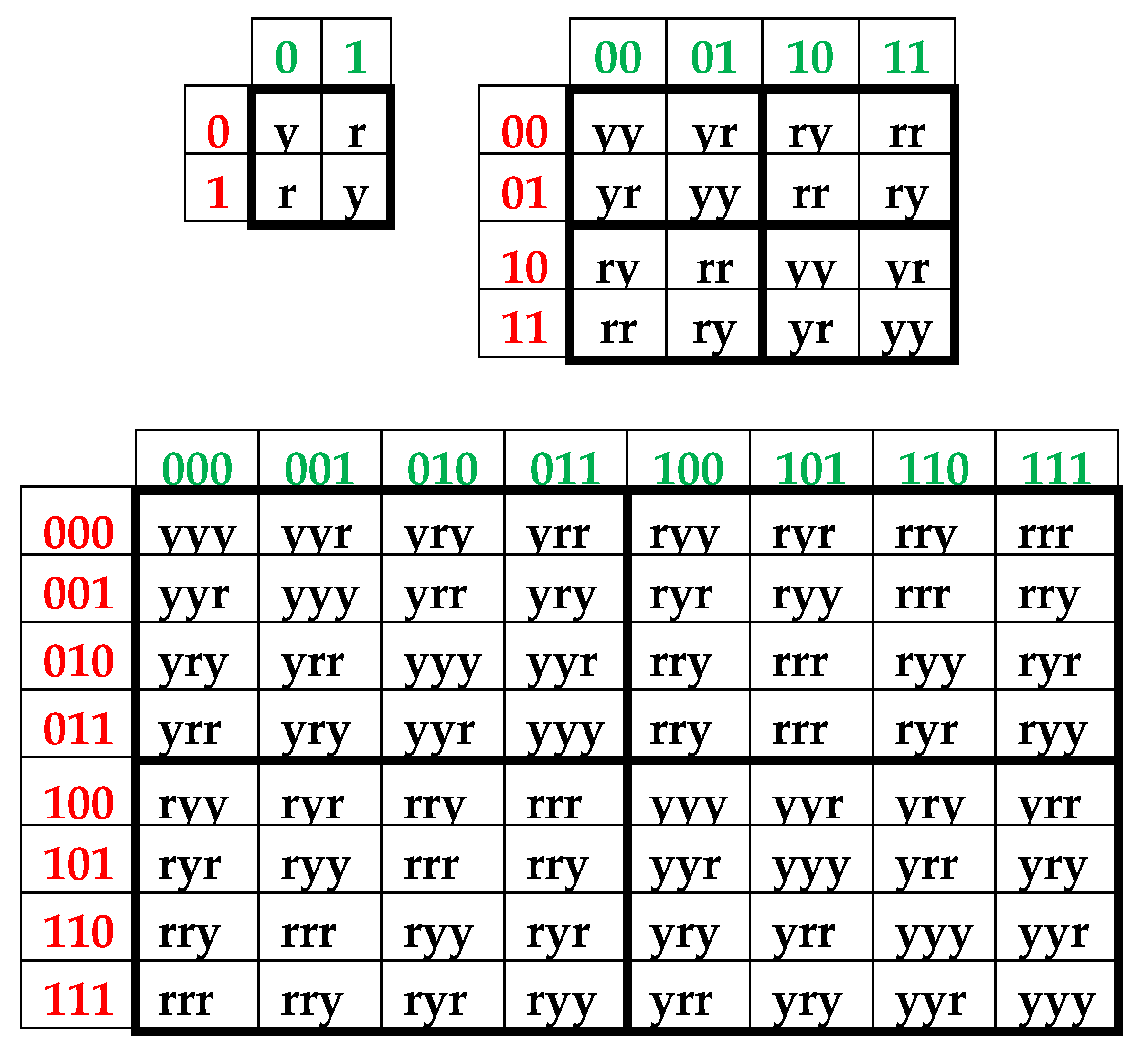
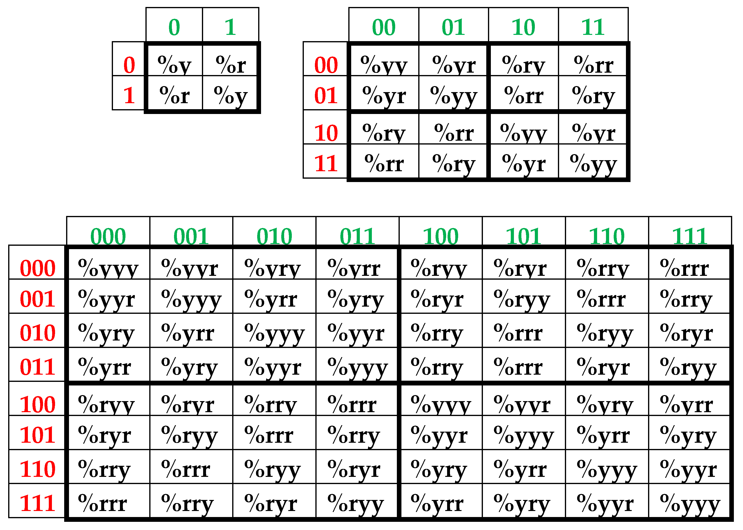
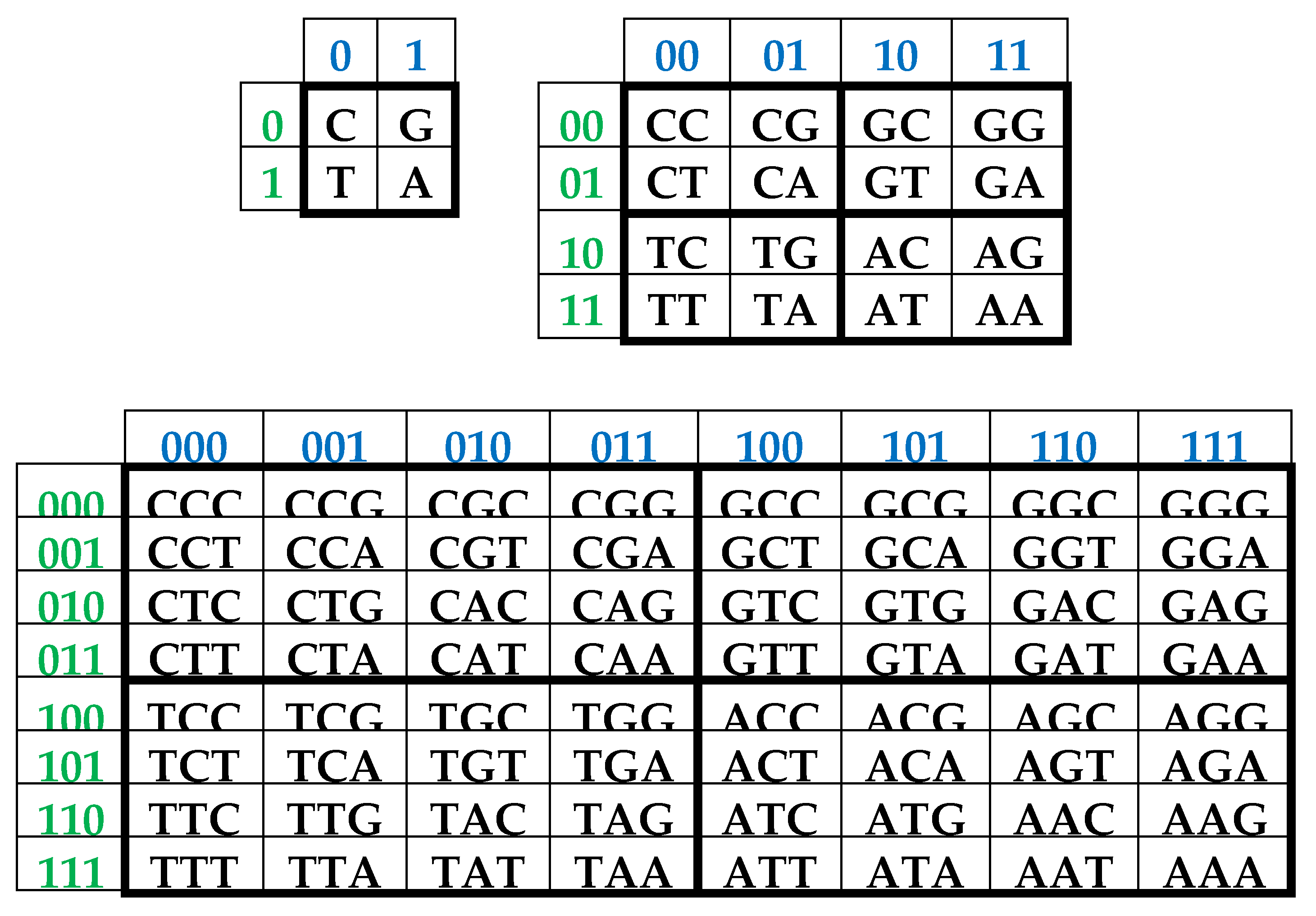
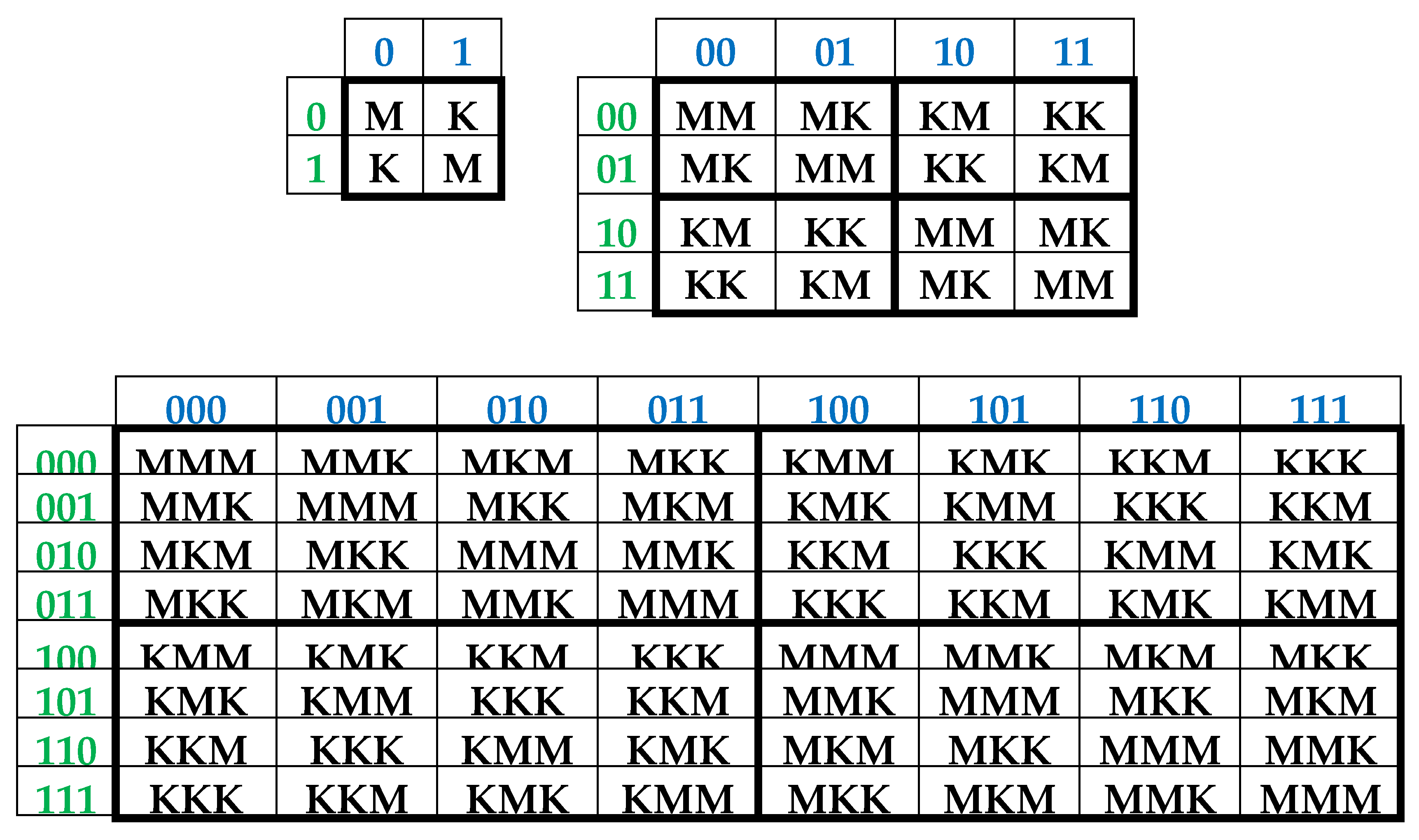
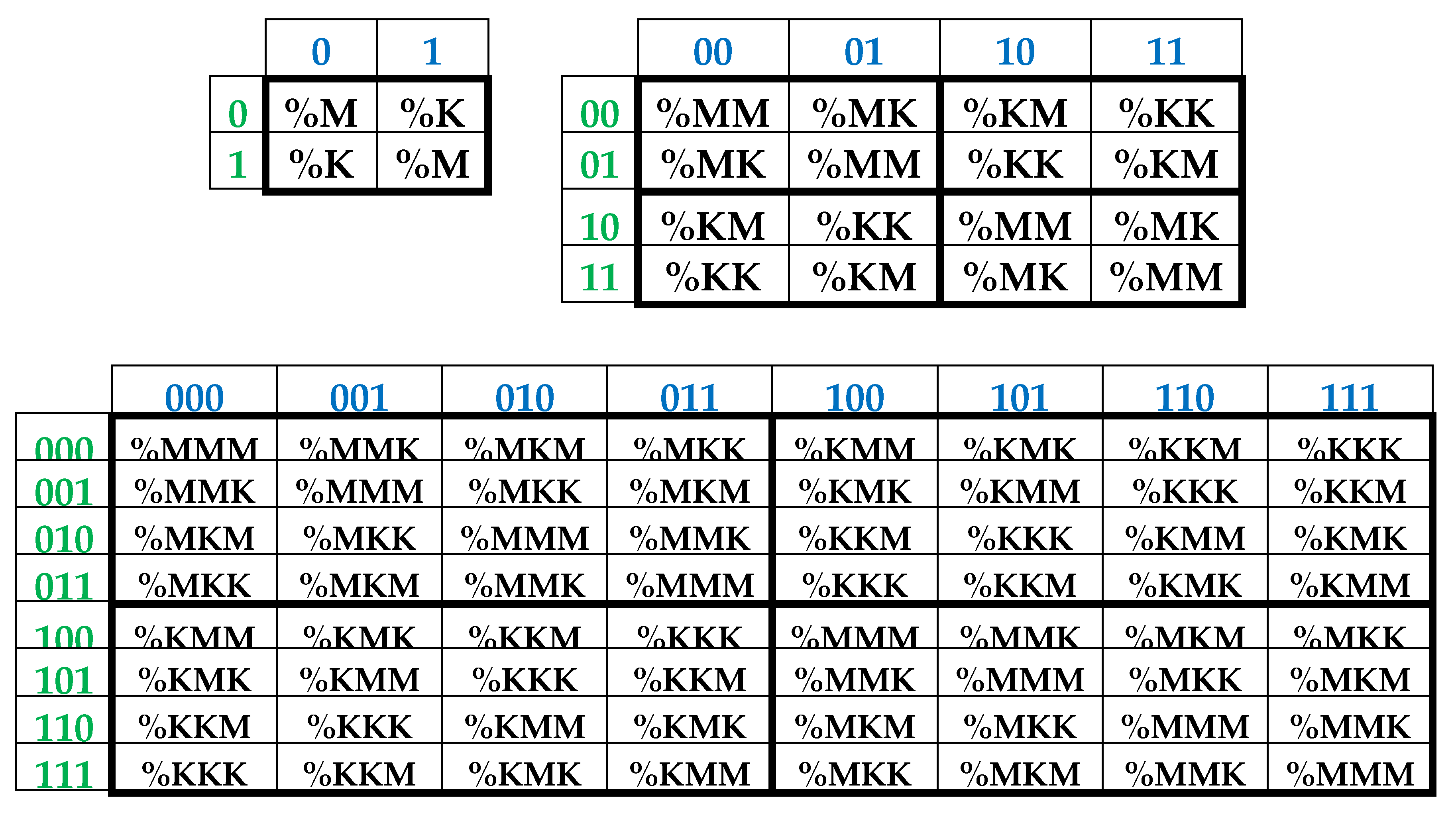
It is convenient to represent DNA-alphabets of 4 nucleotides, 16 doublets, 64 triplets, …, 4ⁿ n-plets in a form of appropriate square tables (~~Figure 1~~), whose rows and columns are enumerated by binary symbols in line with the following principle. Entries of each column are enumerated by binary indicators “pyrimidine or purine” (C = T = 0, A = G = 1); for example, the triplet CAG and all other triplets in the same column are the combinations “pyrimidine-purine-purine” and so this column is correspondingly enumerated 011. By contrast, entries of each row are numerated by binary indicators “amino or keto” (C = A = 0, T = G = 1); for example, the same triplet CAG and all other triplets in the same row are the combination “amino-amino-keto” and so this row is correspondingly numerated 001. In such alphabetic tables (~~Figure 1~~), each of 4 letters, 16 doublets, 64 triplets, … takes automatically its own individual place and all components of these alphabets are arranged in a strict order. This strict ordering of the relative positions of all members of the DNA alphabets proves useful in revealing hidden regularities and rules in the genetic coding system. As it is known, these three separate genetic tables (~~Figure 1~~) form the joint tensor family of matrices [C, A; T, G]⁽ⁿ⁾, where the symbol (n) refers to tensor power n, since they are interrelated by the known operation of the tensor (or Kronecker) product of matrices [Petoukhov, 2008].

One can see in Figure 1, that all complementary n-plets are located inverse-symmetrically with respect to the center of the appropriate matrix. Correspondingly, the 2n-bit binary numbering of each n-plet is transformed into 2n-bit numbering of its complementary n-plet (that is, n-plet of the opposite strand of DNA) by the mutual interchanging of digits 0↔1 in it. For example, by this complementary operation, the numbering 001010 of the triplet CAT becomes the numbering 110101 of its complementary triplet GTA. This interchanging 0↔1 is called the complementary operation and is actively used below in the theme of a realization of the ancient principle “like begets like” in matrix genetics.

The presentation of ensembles of elements of the genetic coding system in the form of tensor families of genetic matrices has appeared as a useful tool to investigate structures of the genetic code from the viewpoint of their analogy with the theory of discrete signals processing, noise-immunity coding, quantum informatics, etc. The scientific direction, which deals with such matrix presentation of the ensembles of genetic elements and their numeric parameters, is named “matrix genetics’ [Petoukhov, 2008; Petoukhov, He, 2010].

3. Complementary-replicated genetic matrices and the even-odd columns decomposition of the matrix of 64 triplets

As one can see from Figure 1, binary numberings of columns and rows of the (2ⁿ*2ⁿ)-matrices of DNA alphabets belong to dyadic groups of binary numbers. For example, in the (8*8)-matrix of 64 triplets, its columns and rows are numerated by 3-bit binary numbers forming the corresponding dyadic group (1):

001, 000, 011, 010, 101, 100, 111, 110

(1)

This series (1) is a particular example of dyadic groups, in which modulo-2 addition serves as the group operation [Harmuth, 1989]. The distance in dyadic groups is known as the Hamming distance. Since the Hamming distance satisfies the conditions of a metric group, the dyadic group is a metric group. The modulo-2 addition of any two binary numbers from (1) always results in a new number from the same series. The number 000 serves as the unit element of this group: for example, 010 ⊕ 000 = 010. The reverse element for any number in this group is the number itself: for example, 010 ⊕ 010 = 000.

Two binary numbers that are converted into each other under inter-replacing 0↔1 will be called complementary. For example, in the dyadic group (1), the pairs of complementary numbers are the following: 000-111, 001-110, 010-101, 011-100 (in the decimal system, they correspond to pairs of numbers 0-7, 1-6, 2-5, 3-4). In a pair of complementary numbers, one of them is always even and the other is odd, that is, any pair of complementary numbers is the pair of even and odd numbers (or Yin and Yang numbers in line with ancient Chinese notions). Accordingly, any two columns (rows) that are enumerated by complementary binary numbers are called complementary. In the genetic matrices in Figure 1, complementary columns are located mirror-symmetrical in the left and right halves of the matrices, and complementary rows are located mirror-symmetrical in the upper and lower halves.

One should emphasize that, in the matrix in Figure 1 and Figure 2, any column enumerated by even number contains only triplets ending by pyrimidines C or T; in contrast, any column enumerated by odd number contains only triplets ending by purines A or G. The mentioned numeric inter-replacing 0↔1 in numberings of columns symbolizes the molecular inter-replacing: it means the transition from columns with triplets ending in pyrimidines to columns with triplets ending in purines and vice versa. Similarity to this, any row enumerated by even number contains only triplets ending by amino-molecules A or C; in contrast, any row enumerates by odd number contains only triplets ending by keto-molecules G or T. The mentioned numeric inter-replacing 0↔1 in numberings of rows symbolizes the molecular inter-replacing: it means the transition from rows with triplets ending in amino-molecules to rows with triplets ending in keto-molecules and vice versa.

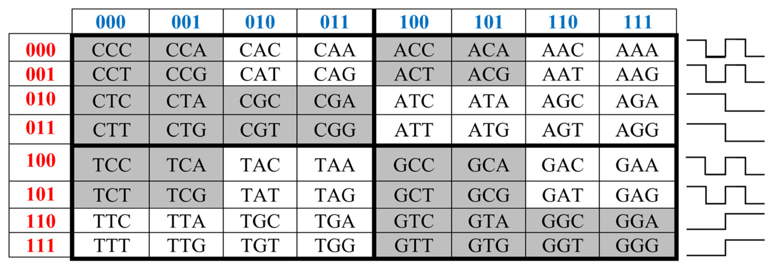
Let us remind one more phenomenological symmetry connected with the known binary-oppositional separation of the DNA alphabet of 64 triplets - according to their code properties - into two equal sub-alphabets: 32 triplets with strong roots (i.e. triplets starting with 8 strong duplets CC, CT, CG, AC, TC, GC, GT, GG) and 32 triplets with weak roots (i.e. triplets starting with other 8 duplets) [Rumer, 1968; Fimmel, Strüngmann, 2016]. Coding value of triplets with strong roots is independent of a letter on their third position. For example, the four triplets with the same strong root CGC, CGA, CGT, CGC encode the same amino acid Arg, though they have different letters on their third position. By contrary, the coding value of triplets with weak roots depends on a letter on their third position. For example, in the grouping of the four triplets with the same weak root CAC, CAT, CAA, and CAG, two triplets (CAC, CAT) encode the amino acid His and the other two (CAA, CAG) encode another amino acid Gln. In Figure 2, which repeats Figure 1 in some detail, all triplets with strong roots are marked by black color in contrast to triplets with weak roots denoted by white color.

In the matrix in Figure 2, a sequence of black and white cells in each row has a meander-like character: black fragments and white fragments have identical length. Such mosaic of each row corresponds to a meander-like form of one of Rademacher functions that take only two values «+1» and «-1» and whose examples are shown in Figure 2. Rademacher functions are connected with the theory of orthogonal series and theory of probabilities. For example, every statement about the Rademacher functions can be interpreted from the point of view of the theory of probability (see details in [Alexits, 1961, §7; Petoukhov, 2021b]).

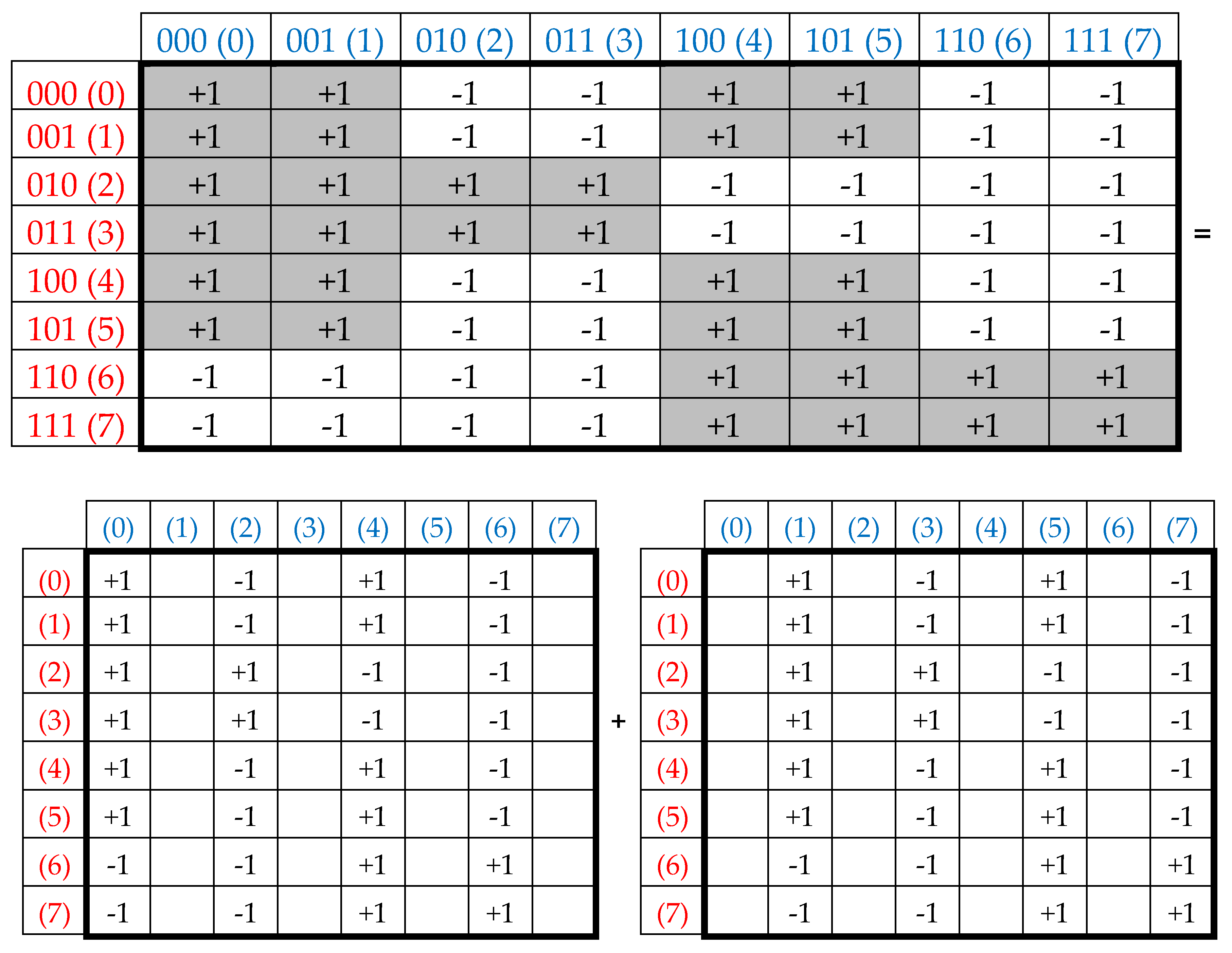
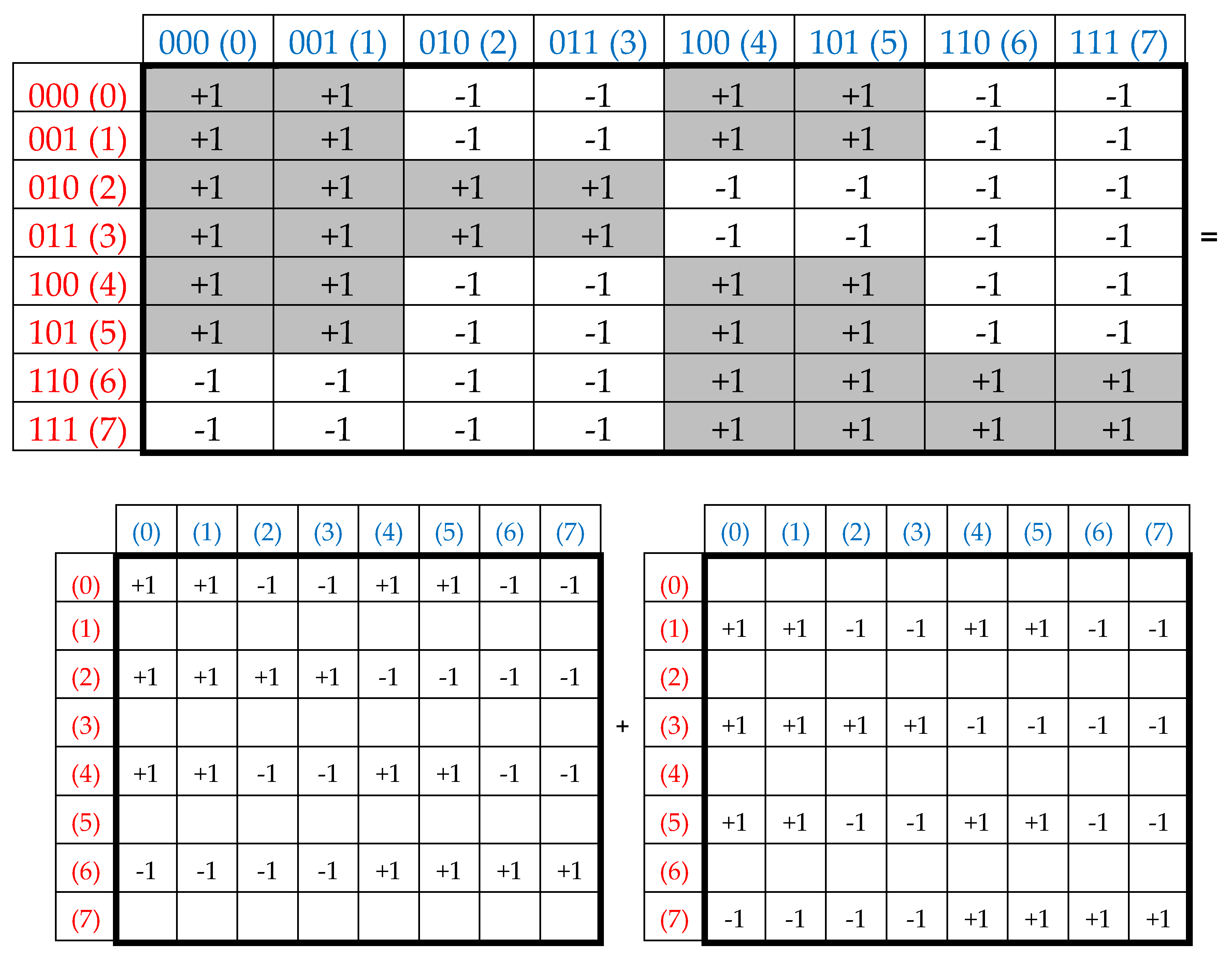
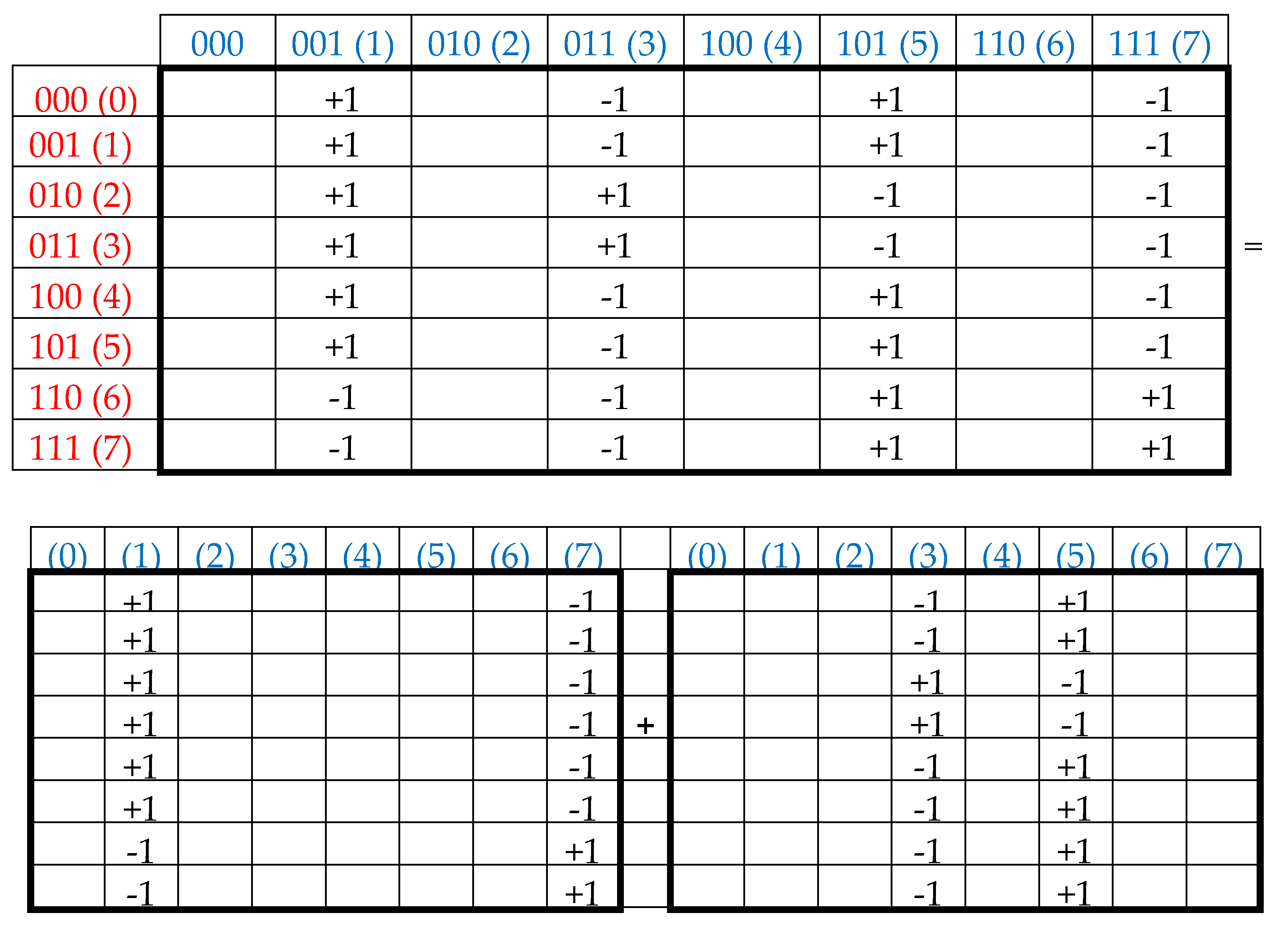
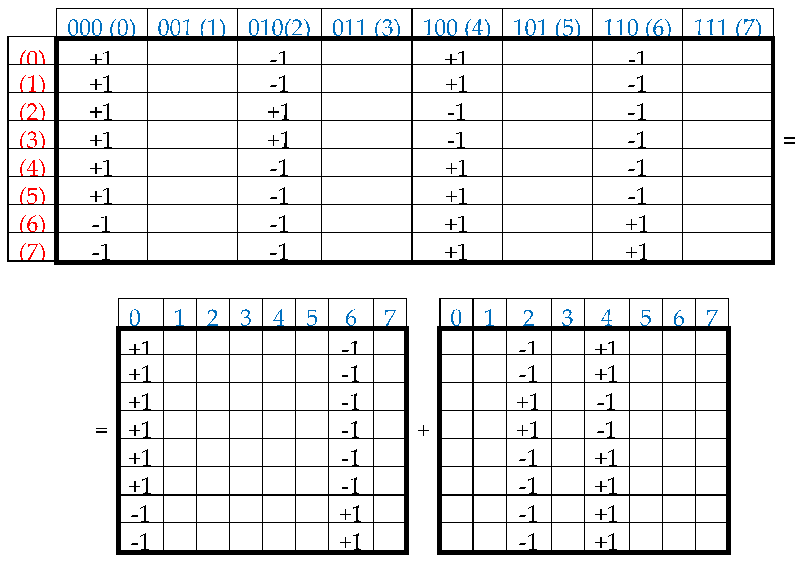
Black and white cells of the symbolic matrices in Figure 2 reflect the binary opposition of triplets with strong and weak roots and therefore can be represented by elements +1 and -1 in them. In this representation, a numeric matrix appears (Figure 3, at top). Since this numerical matrix is closely related to the Rademacher functions, it is conventionally called Rademacher genetic matrix of 64 triplets. Does this Rademacher genetic matrix have any essential algebraic meaning? Yes, it has. Let us show this.

This Rademacher genetic matrix is a sum of two sparse matrices shown in Figure 3 at bottom. One of these sparse matrices, called as an even-columns matrix, contains only columns with even numberings; the second sparse matrix, called as an odd-columns matrix, contains only columns with odd numberings.

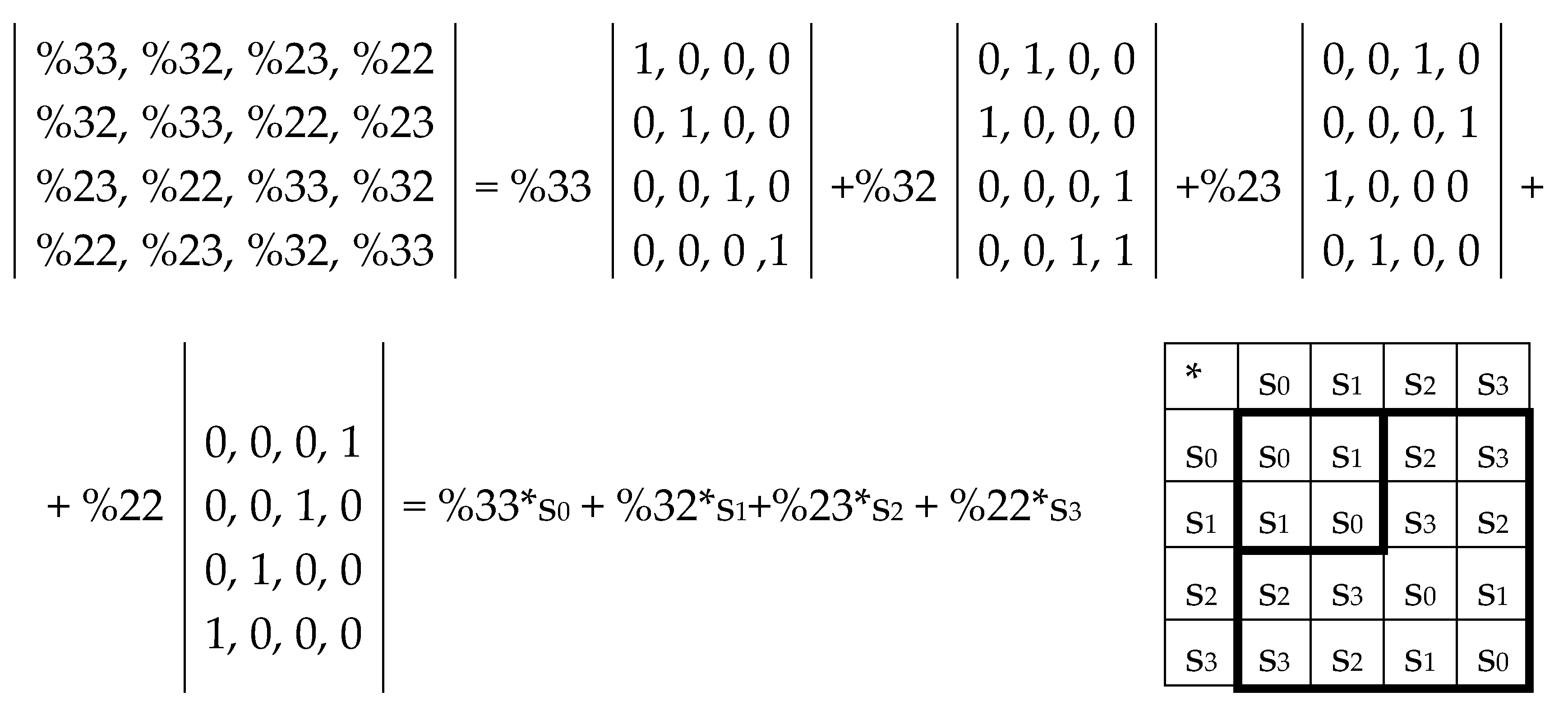
The even-columns (8*8)-matrix in Figure 3 is the sum of 4 sparse (8*8)-matrices s₀+s₁+s₂+s₃ shown in Figure 4 (such decomposition is conditionally called the column dyadic-tensor-shift decomposition since it is associated with the well-known dyad-shift decomposition of matrices [Ahmed, Rao, 1975], which has undergone a certain complication based on the tensor product). The set of these 4 matrices s₀, s₁, s₂, s₃ is closed relative to multiplication and corresponds to a certain multiplication table in Figure 4, at right. This table matches to the multiplication table of the 4-dimensional algebra of Cockle split-quaternions [https://en.wikipedia.org/wiki/Split-quaternion], which is used in the Poincare conformal disk model of hyperbolic geometry [Karzel, Kist, 1985]. Some connections of hyperbolic geometry with structural peculiarities of inherited physiological systems were described in [Bodnar, 1992, 1994; Kienle, 1964; Petoukhov, 1989; Smolyaninov, 2000].

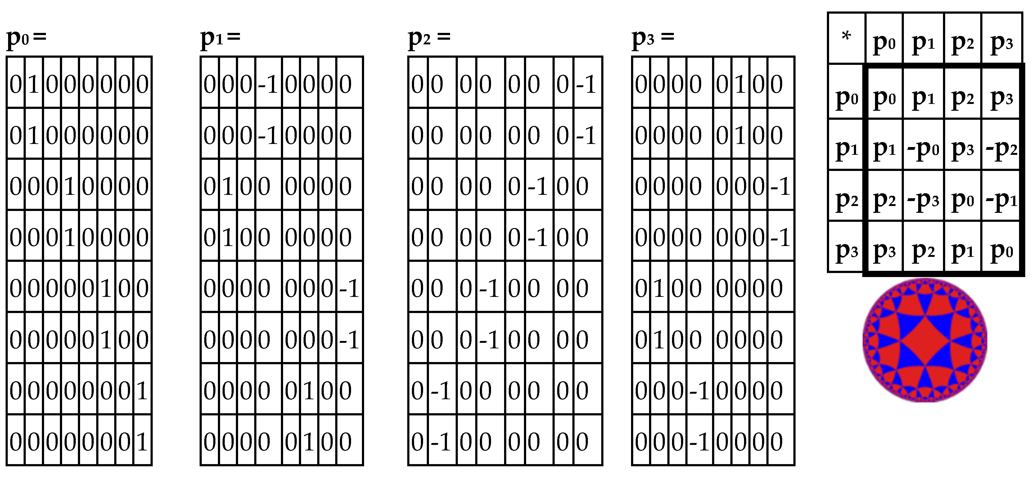
Analogically, the odd-columns matrix (Figure 3, at right) is the sum of 4 sparse matrices p₀+p₁+p₂+p₃ shown in Figure 5. The set of these 4 matrices p₀, p₁, p₂, p₃ is closed regarding multiplication and defines the multiplication table in Figure 5, at right. This multiplication table coincides with the multiplication table of the 4-dimensional algebra, which was received above for the even-columns matrix (Figure 4). Both the even-columns matrix and the odd-columns matrix present Cockle’s split-quaternions with unit coordinates (these split-quaternions have different forms of their matrix representations, with which these even-columns and odd-columns genetic matrices turn out to be associated). Correspondingly, both these genetic matrices are connected with the Poincare conformal disk model of hyperbolic geometry.

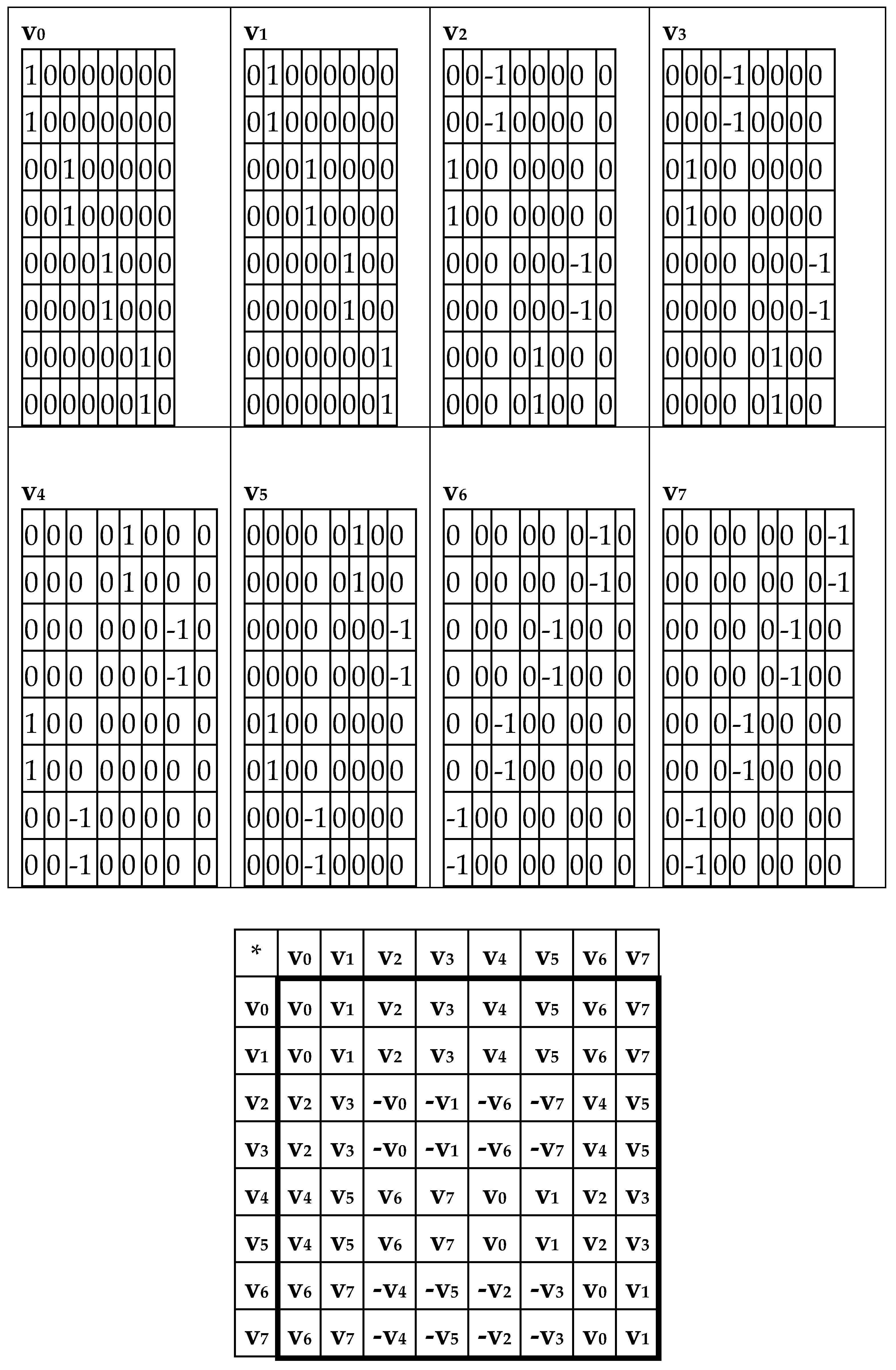
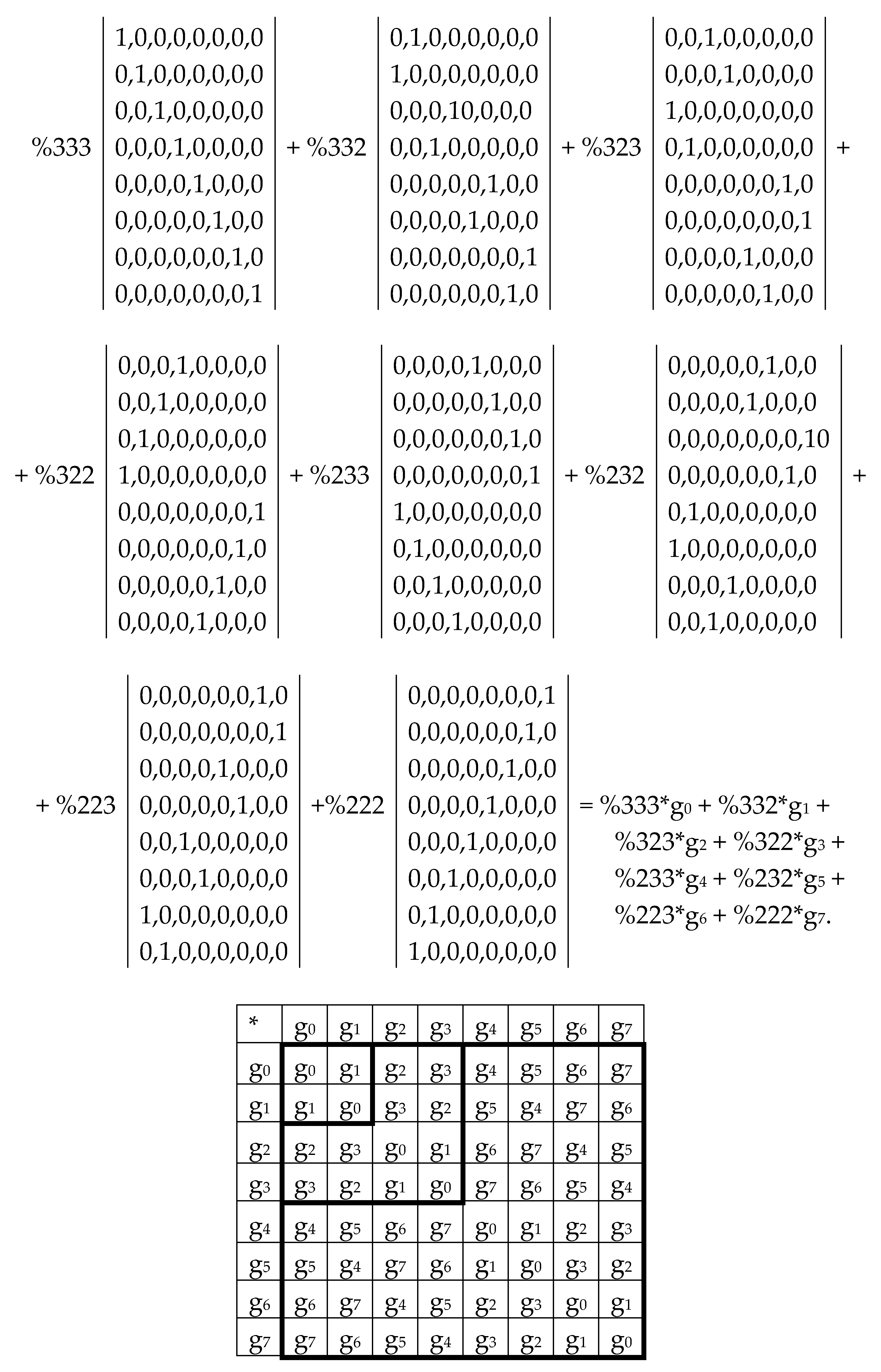
Now let us show that the summation of the even-columns and odd-columns matrices, which are complementary to each other and connected with the 4-dimensional algebra, gives the combined matrix W as a new algebraic entity, which is connected already with the 8-dimensional algebra. This combined matrix (Figure 3 and Figure 5) - under its column dyadic-tensor-shift decomposition – is the sum of 8 sparse matrices v₀+v₁+v₂+v₃+v₄+v₅+v₆+v₇ shown in Figure 6. The set of these matrices v₀, v₁, v₂, v₃, v₄, v₅, v₆, v₇ is closed relative to multiplication and matches to the multiplication table (Figure 6, at the bottom) of a certain 8-dimensional algebra. This algebra has interesting properties, which were described in previous publications without a connection with the presented topic of complementary replications [Petoukhov, 2008a-c; Petoukhov, He, 2010].

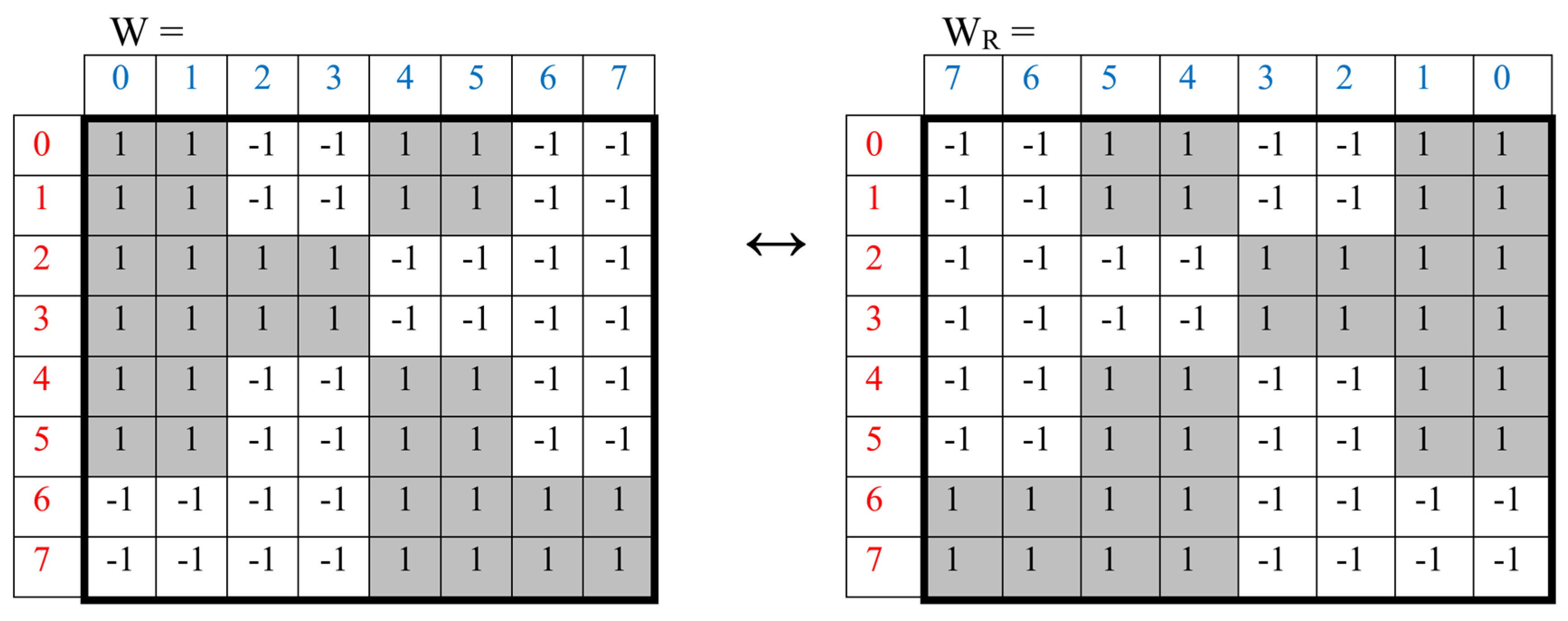
This summary matrix W generates algorithmically its complementary-replicated analogue W_R by means of the interchange of numbers 0↔1 in the binary numerating of its columns with the corresponding rearrangement of the columns (that is, rearrangements of columns located mirror symmetrically in the left and right halves of the matrix). This interchanging algorithm 0↔1 in binary numbers provides interchange in any pair of complementary columns that differ from each other in the content of triplets with purine and pyrimidine endings, in some analogy with the complementarity of purines and pyrimidines in DNA double strands. For example, the column with number 110 (which corresponds to the nucleotide order “purine-purine-pyrimidine” in all its triplets) takes the place of the column with number 001 (which corresponds to the order “pyrimidine-pyrimidine-purine” in all its triplets). Figure 7 shows the summary matrix W and its complementary-replicated analogue W_R, which is generated by this algorithm based on binary-oppositions in the DNA nucleobases alphabet and which is also connected by its meander like mosaic with meander-like Rademacher functions.

Applying this complementary-replicating algorithm to the complementary-replicated matrix W_R generates the original Rademacher matrix W, that is, matrices W and W_R is mutual complementary-replicated matrices resembling two complementary strings of DNA. This algorithm is recursive and its applying allows generating such pairs of complementary-replicated matrices again and again. So, the ancient notions that “like begets like” surprisingly turn out to be realized in genetics not only for complementary strings of DNA but also for the phenomenological structure of the genetic matrix presented properties of the alphabet of 64 triplets. In other words, molecular complementary-replicated properties of DNA strings exist jointly with algebraic complementary-replicated properties of the considered alphabetical matrices of the genetic code. Both of these properties are parts of genetics of the whole organisms and so interrelated. These algebraic complementary-replicated properties of genetic matrices allow applying effective algebraic methods for further study of genetics to include it in the field of modern mathematical natural sciences in connection with multi-dimensional algebras, hyperbolic geometry, theory of resonances, etc.

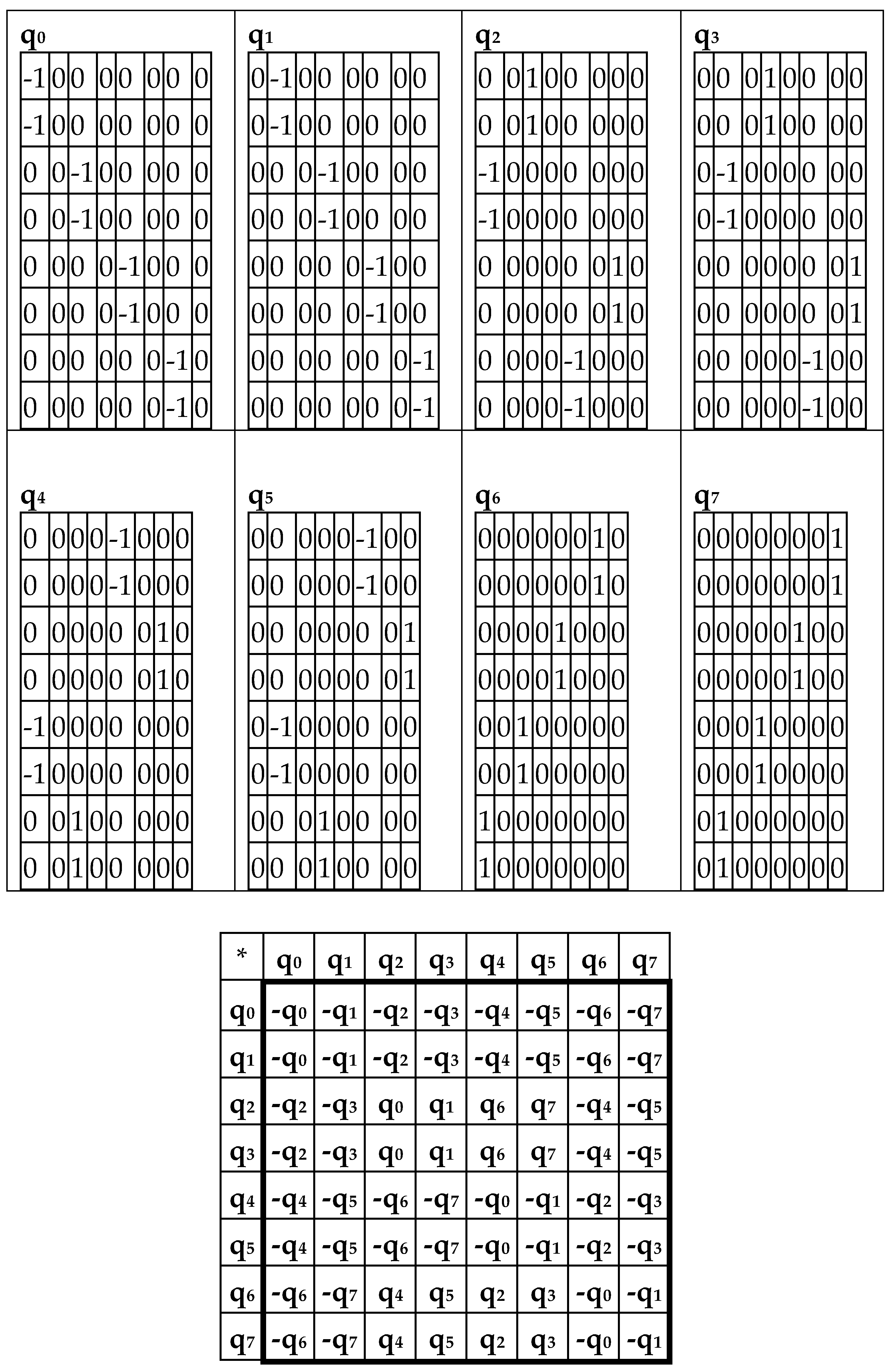
The complementary-replicated matrix W_R – under its column dyadic-tensor-shift decomposition – is the sum of 8 sparse matrices q₀+q₁+q₂+q₃+q₄+q₅+q₆+q₇ shown in Figure 8. The set of these matrices q₀, q₁, q₂, q₃, q₄, q₅, q₆, q₇ is closed relative to multiplication and matches to the multiplication table (Figure 8, at bottom) of a certain 8-dimensional algebra. This new multiplication table is a complementary analogue of the multiplication table shown for the similar decompositions of the matrix W in Figure 6: in these multiplication tables, each value of the multiplication q_i*q_k is equal to the value v_i*v_k but taking with an opposite sign (here indexes i, k = 0, 1, 2, 3, 4, 5, 6, 7).

The action of complementary-replicated (8*8)-matrices W and W_R on an arbitrary 8-dimensional vector

\bar{X}

generates two new vectors that are complementary to each other: the corresponding coordinates of both generated vectors are the same in their absolute values, but have opposite signs. A numerical example of this with a voluntary vector

\bar{X}

= [1, 2, 3, 4, 5, 6, 7, 8] is shown by expression (2):

\bar{X} * W = [1, 2, 3, 4, 5, 6, 7, 8] * W = [6, 6, - 22, - 22, 22, 22, - 6, - 6] = \bar{Y}

\bar{X} * W_{R} = [1, 2, 3, 4, 5, 6, 7, 8] * W_{R} = [- 6, - 6, 22, 22, - 22, - 22, 6, 6] = - \bar{Y}

(2)

Another interesting property of the Rademacher genetic complementary-replicated matrices W and W_R is that - by their repeated action on the emerging vectors (2) - one can generate as many complementary-replicated vectors as desired. In this case, the quadrupling of coordinate values in the vectors occurs, reminiscent of the quadrupling of genetic information during the meiosis division of germ cells, under which one cell generates 4 similar cells with a complete set of DNAs in each. The following example (3), using the denotations from (2), illustrates this quadrupling of coordinate values with a regular changing of signs “+” and “–”:

\bar{Y} * W_{R} = - 4 * \bar{Y}; \bar{Y} * {W_{R}}^{2} = 4^{2} * \bar{Y}; \bar{Y} * {W_{R}}^{3} = - 4^{3} * \bar{Y}; \bar{Y} * {W_{R}}^{4} = 4^{4} * \bar{Y}; etc.

(3)

The expression (4) shows one more property of the Rademacher complementary-replicated matrices W and W_R:

W*W_R = W_R*W = -4W_R

(4)

The matrix W/4 is an oblique projector since (W/4)² = W/4. In contrast, the matrix W_R corresponds to another condition: (W_R/4)² = -W_R/4.

Each of the resulting vectors

\bar{X}

*W and

\bar{X}

*W_R is always a complementary palindrome: the sequence of its coordinates, which is read in forward order, coincides with the sequence, which is read in reverse order and has coordinates with the opposite sign (see the example (2)). This algebraic feature of the action of complementary-replicated matrices on voluntary vectors is interesting, since in molecular genetics the problem of complementary palindromes has long been known. Here one should remind about the difference in notions of an ordinary palindrome and a complementary palindrome. By definition, an ordinary palindrome is a string that reads the same from beginning and from the end. By contrast, a complementary palindrome in molecular genetics is a fragment of a chain of DNA or RNA, which becomes an ordinary palindrome, if each symbol in one half of the fragment is replaced by its complementary symbol (A

\leftrightarrow

T, C

\leftrightarrow

G) [Gusfield,1997]. For instance, AGCTCGCGAGCT is a complementary palindrme. In nucleotide sequences of DNA and RNA, a great number of complementary palindromes and ordinary palindromes exists [Gusfield, 1997; Lehninger, 1982]. For instance, families of repetitive sequences occupy about one-third of the human genome. The importance of the problem of repeats in genetic sequences is reflected in the fact that during 20 years before 1991 on this subject was published 6000 articles [Gribskov, Devereux, 1991].

One should add that the theme of the complementary columns (and rows) in the described genetic matrices is also essential in connection with the universal rules of stochastic organization of DNA in genomes of higher and lower organisms [Petoukhov, 2022a,b]. These rules include approximate equalities of sums of probabilities of triplets belonging to the even column and the odd column of each pair of complementary columns (the same is true for each pair of complementary rows).

4. Complementary-replicated genetic matrices and the even-odd rows decomposition of the matrix of 64 triplets

Let us show that similar algebraic results arise in the case of “the rows dyadic-tensor-shift decomposition” of the same mosaic matrix of 64 triplets from Figure 3. This matrix has pairs of complementary rows, which are located mirror-symmetrical in its top and bottom halves; as it was noted above, each of such pair contains one row with even number and one row with odd number. Figure 9 shows that the numeric presentation of this matrix, containing entries +1 and -1 (whose locations correspond to triplets with strong and weak roots), is the sum of two sparse matrices, one of which contains only non-zero rows enumerated by even numbers and the other contains only non-zero rows enumerated by odd numbers. Each of the pairs of complementary rows is separated among these two matrices. Correspondingly, the sparse matrix with even-numerated rows is conditionally called the even-rows matrix of the row type; all its non-zero rows correspond to triplets, which contain amino-molecules A or C at their ends (by this reason, this sparse matrix can be also called the amino-rows matrix). The sparse matrix with odd-numerated rows is called the odd-rows matrix; all its non-zero rows correspond to triplets, which contain keto-molecules G or T at their ends (by this reason, this sparse matrix can be also called the keto-rows matrix).

The even-rows (8*8)-matrix in Figure 9 is the sum of 4 sparse (8*8)-matrices u₀+u₁+u₂+u₃ shown in Figure 10. The set of these 4 matrices u₀, u₁,u₂, u₃ is closed relative to multiplication and corresponds to a certain multiplication table in Figure 10 at right. This table is again the multiplication table of the 4-dimensional algebra of Cockle split-quaternions, which we met above in Figure 4 and Figure 5 and which is used in the Poincare conformal disk model of hyperbolic geometry.

Analogically, the odd-rows matrix (Figure 9, at right) is the sum of 4 sparse matrices a₀+a₁+a₂+a₃ shown in Figure 11. The set of these 4 matrices a₀, a₁, a₂, a₃ is closed regarding multiplication and defines the multiplication table in Figure 11, at right. This multiplication table coincides with the multiplication table of the 4-dimensional algebra, which was received above for the even-rows matrix (Figure 10) and for even-columns and odd-columns matrices (Figure 4 and Figure 5). Both the even-rows matrix and the odd-rows matrix represent Cockle’s split-quaternions with unit coordinates, which are connected with the Poincare conformal disk model of hyperbolic geometry.

The sum of the even-rows matrix and the odd-rows matrix gives the genetic matrix W in Figure 3 at top, which was above analyzed jointly with its complementary-replicated analogue W_R (Figure 6, Figure 7 and Figure 8).

Similar approaches using even-odd structures and dyadic-tensor-shift decompositions are also appropriate to analyze complementary replicated properties of Rademacher genetic matrices of higher orders, for example, the (16*16)-matrix of 256 tetraplets.

Different forms of implementation of the fundamental biological principle “like begets like” (or a complementary replication in a wide sense) can be seen at different levels of inherited biological organization. For example, in the brain of humans and animals, which has mirror complementary hemispheres (left and right), mirror neurons are known. A mirror neuron is a neuron that fires both when an animal acts and when the animal observes the same action performed by another. Thus, the neuron “mirrors” the behavior of the other, as though the observer were itself acting.

The theme of mirror neurons, whose functioning is based on one of the forms of the principle “like begets like”, provokes wide scientific researches and debates since it concerns cognitive functions, an origin of language, learning facilitation, automatic imitation, motor mimicry, autism, human capacity of emotions such as empathy, and many other problems (see for example [Morsella, Bargh, Gollwitzer, 2009; Rizzolatti, Sinigaglia, 2008]). In 2014, Philosophical Transactions of the Royal Society B published a special issue entirely devoted to mirror neuron research [Ferrari, Rizzolatti, 2014]. One of the arisen questions is the following: where do mirror neurons come from? [Heyes, 2010].

The above-described results of our studies in the field of matrix genetics give pieces of evidence that the system of mirror neurons and the system of DNAs complementary replication are not isolated parts of the organism, but they are particular parts of a bio-algebraic complex realizing inherited phenomena “like begets like”. Other examples of manifestation of this complex are, for example, structured DNA alphabets in their matrix representation forms, as well as universal rules for even-odd stochastic organization of genomic DNAs of higher and lower organisms [Petoukhov, 2022a,b]. Our body structure with its left and right halves, having left-and-right sensory-motor systems, also can be considered as one of the manifestations of this complementary-replicating complex. Another example is given by our visual perception whose optical system of the eye provides the transmission of the external image to the retina in complementary inverted and reduced forms. Although the image on the retina is inverted, we can see objects in a direct form by some complementary-replicating action of our brain.

Correspondingly, complementary replication is a systemic phenomenon in the genetic organization. It’s not that the molecules of two strands of DNA randomly docked, formed a complementary pair and began to repeat the process of complementary replication at breakneck speed. Another point of view is proposed: the DNA filaments replication phenomenon is a part of a holistic bio-algebraic genetic complex of complementary replication, parts of which manifest themselves at different levels of organization of the living, up to the functioning of the brain with its mirror neurons and the ability to empathize and imitate external events. This bio-algebraic complex can be considered as responsible for the implementation of the ancient principle “like begets like” at different levels of biological organization in the course of biological evolution.

5. Complementary replications and the matrix of 64 triplets under its twice-complementary transformation

This section continues research in the field of matrix genetics and phenomena of algebra-biological binary oppositions, aimed at demonstrating the key role of the principle “like begets like” and complementary replications in the genetic coding system including tensor families of genetic matrices.

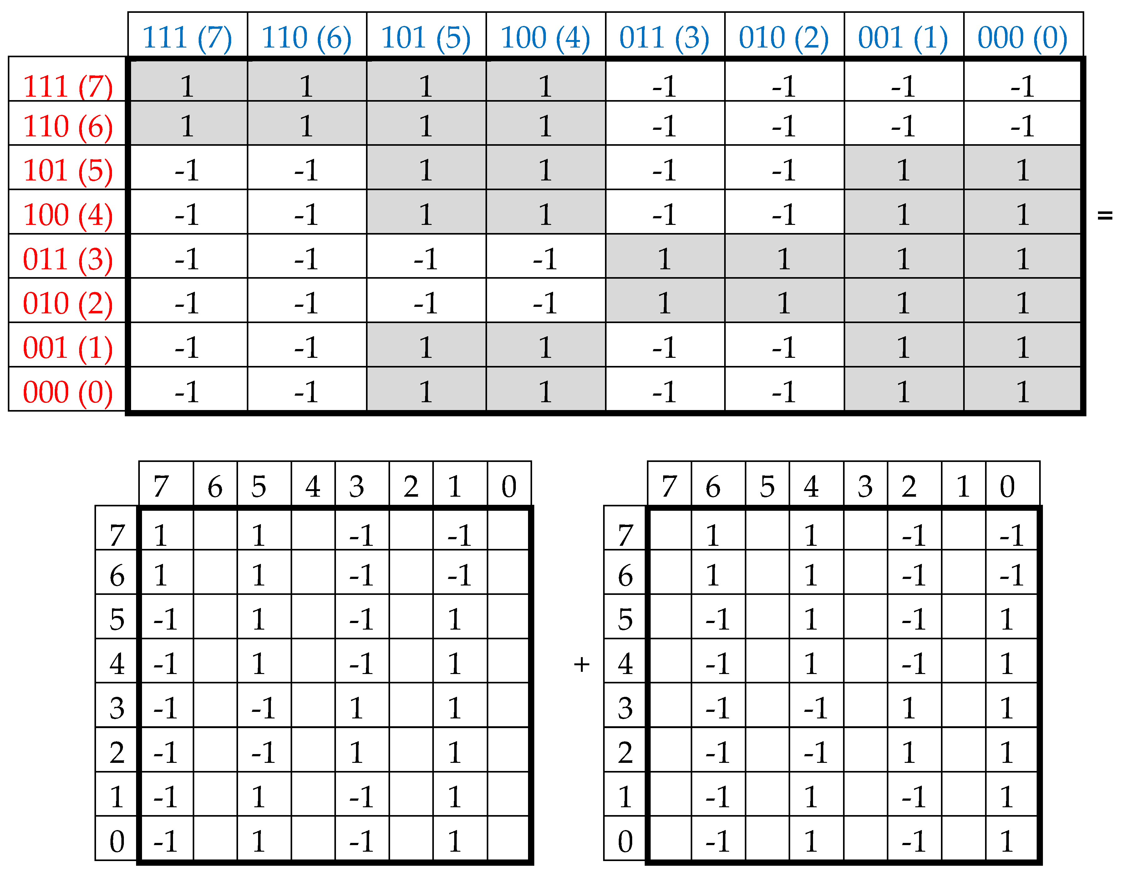
For this additional research, let us consider a transformation of the Rademacher genetic matrix of 64 triplets from Figure 2 under the simultaneous interchange of numbers 0↔1 in the binary numerating of its columns and rows with appropriate rearrangements of the columns and the rows. These rearrangements of numberings correspond to simultaneous molecular interchanges inside all pairs of complementary columns and also all pairs of complementary rows defined above by indicators of purine-pyrimidine endings and amino-keto endings in triplets. Figure 12 shows a new Rademacher matrix B, which arises under such a twice-complementary transformation and which is conditionally called the twice-complementary matrix. This twice-complementary matrix B satisfies the following conditions: B² = 4B, (B/2)² = B/2, that is, the asymmetrical matrix B/2 is an oblique projector. The matrix B is the sum of two matrices: the odd-columns matrix and the even-columns matrix, which are shown in Figure 12, at the bottom.

It turns out that the odd-columns matrix BOC is the sum of 4 new sparse matrices b₀ + b₁ + b₂ + b₃, whose set is closed relative to multiplication and defines a multiplication table of the algebra of split-quaternions of Cockle as it is shown in Figure 13 (compare with Figure 4 and Figure 5). This algebra is used in the Poincare conformal disk model of hyperbolic geometry.

It turns out also that the even-columns matrix BEC (from Figure 12, at bottom right) is the sum of 4 new sparse matrix k₀ + k₁ + k₂ + k₃, whose set is closed relative to multiplication and defines a multiplication table of the algebra of split-quaternions of Cockle as well as it is shown in Figure 14 (compare with the same multiplication table in Figure 4, Figure 5, and Figure 13).

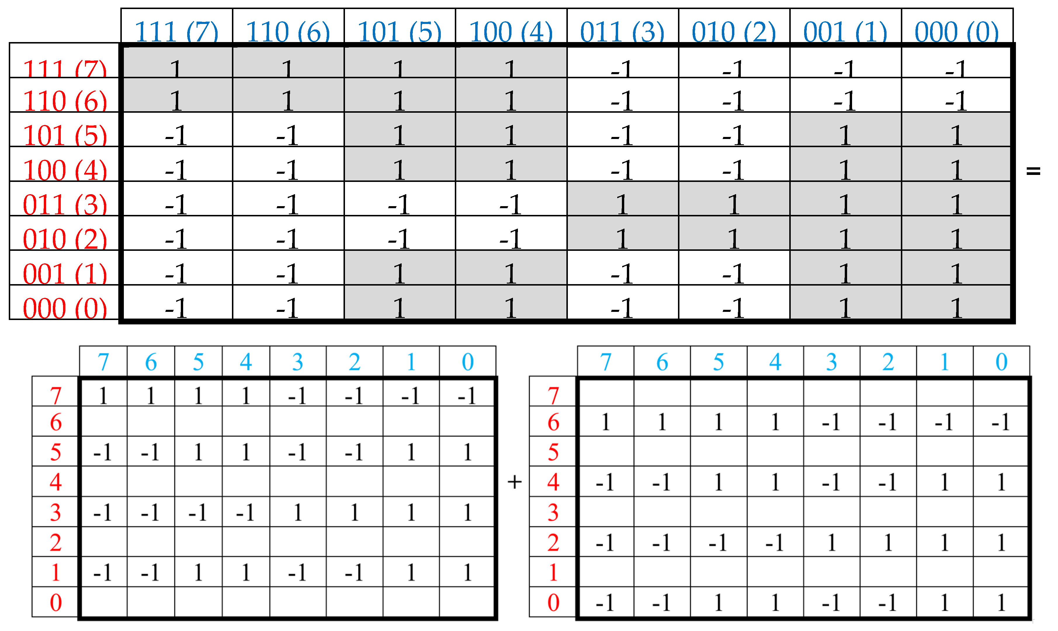
Twice-complementary matrix B (Figure 12, at top) can be also presented as the sum of the odd-rows matrix BOR and the even-rows matrix BER as it is shown in Figure 15.

The odd-rows matrix BOR (Figure 15) is the sum of 4 sparse matrices h₀ + h₁ + h₂ the + h₃, whose set is closed relative to multiplication and defines a multiplication table of the same algebra of split-quaternions of Cockle as it is shown in Figure 16 (compare with the same multiplication table in Figure 4, Figure 5, Figure 13, and Figure 14).

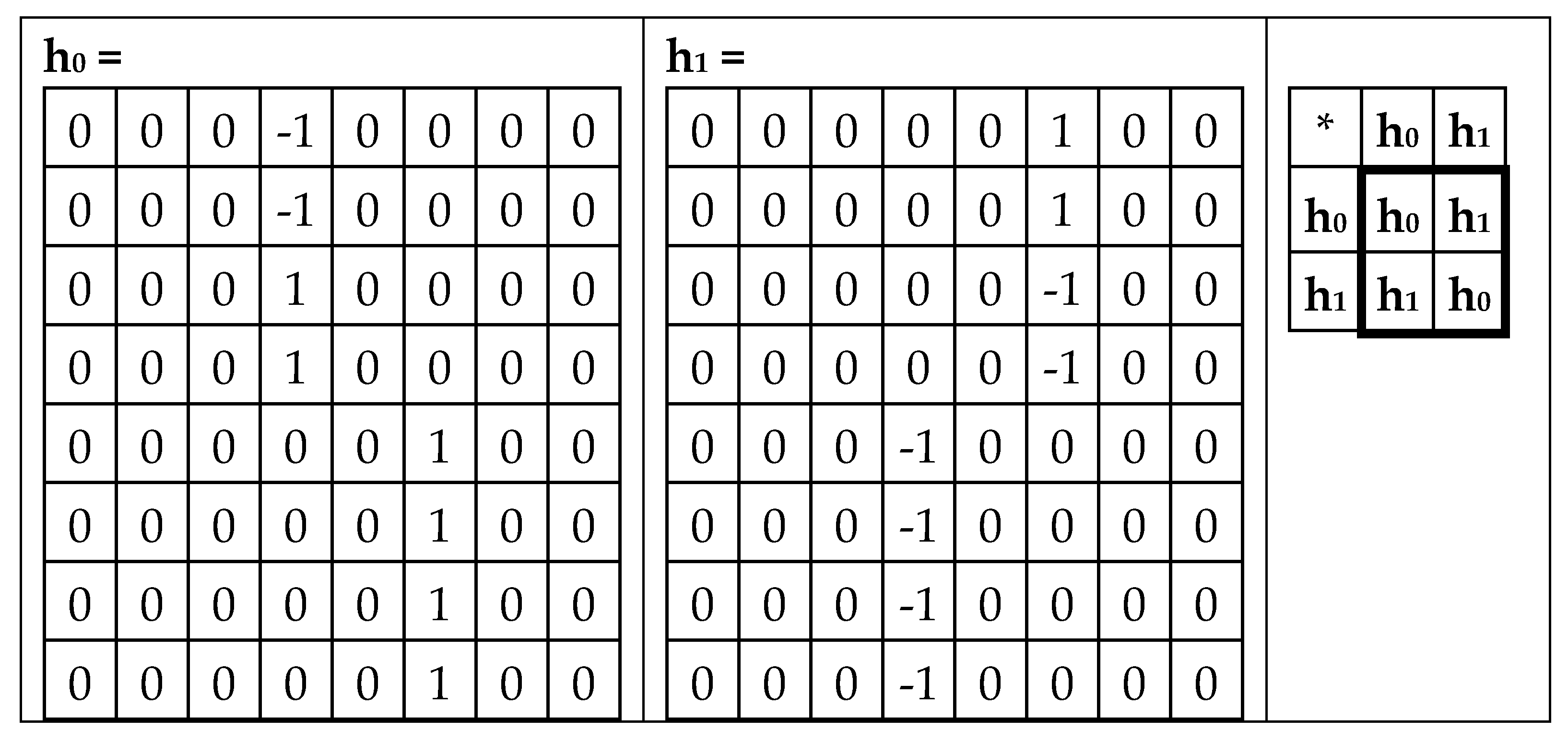
The even-rows matrix BER (Figure 15) is the sum of 4 sparse matrices y₀ + y₁ + y₂ + y₃, whose set is closed relative to multiplication and defines a multiplication table of the same algebra of split-quaternions of Cockle as it is shown in Figure 1.8.6 (compare with the same multiplication table in Figure 4, Figure 5, Figure 13, Figure 14 and Figure 16).

6. Genetic matrices, root-complementarity, and hyperbolic numbers

The materials of sections 4 and 5 do not at all exhaust the vast topic of the implementation of the principle “like begets like” in matrix genetics based on binary oppositions in the structure of the genetic system, including complementary replications in the regular structuring of genetic matrices. This topic should be intensive and systematic studied in future. Here let us show only some additional examples of complementary interrelations in genetic matrices (that is, matrices built on the basis of binary-oppositional properties of the molecular ensembles of the genetic system).

It turns out that introduction of an additional notion of “root-complementarity” is useful for understanding and modeling the non-trivial structurization of a molecular genetic system. By definition, two n-bit binary numbers (n = 3, 4, 5, …) form a root-complementary pair if they transfer each into other under the interchange of numbers 0↔1 only in their roots. For example, such interchanging transforms number 000 into number 110, that is, binary numbers 000 and 110 form the root-complementary pair. Correspondingly, in the genetic matrices, two columns (or rows) form a root-complementary pair if their binary numberings form a root-complementary pair. Below we show that this topic of the root-complementarity pairs is connected with algebra of 2-dimensional hyperbolic (double) numbers.

Let us return to the even-columns matrix in Figure 5, at bottom left. It is the sum of two matrices shown in Figure 18, at bottom. The first matrix contains only two non-zero columns, which are enumerated by root-complementary binary numbers 000 and 110 (that is, numbers 0 and 6 in decimal notation) and is denoted C₀₆. The second matrix contains only two non-zero columns, which are enumerated by root-complementary binary numbers 010 and 100 (that is, numbers 2 and 4 in decimal notation) and is denoted C₂₄.

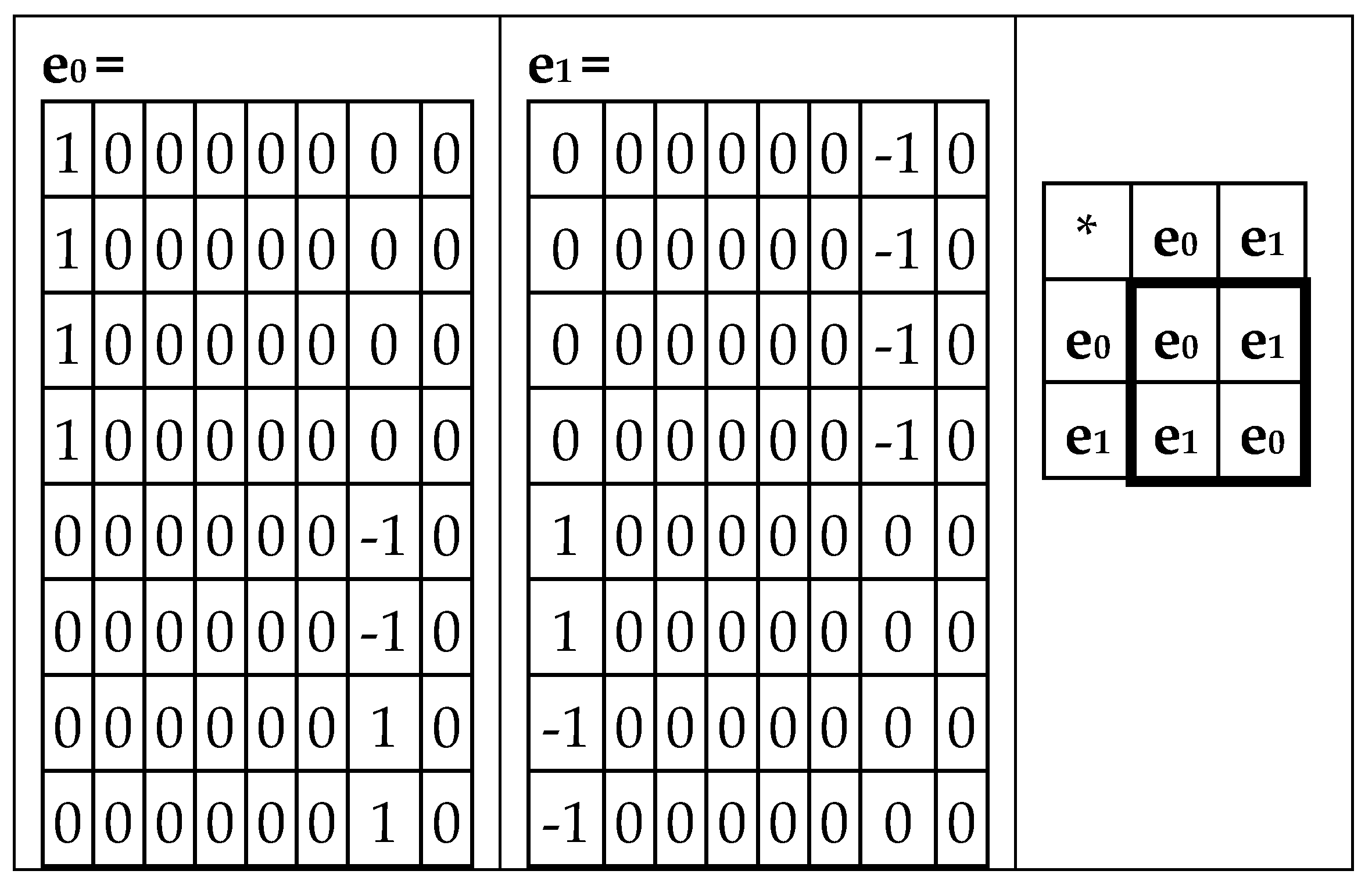
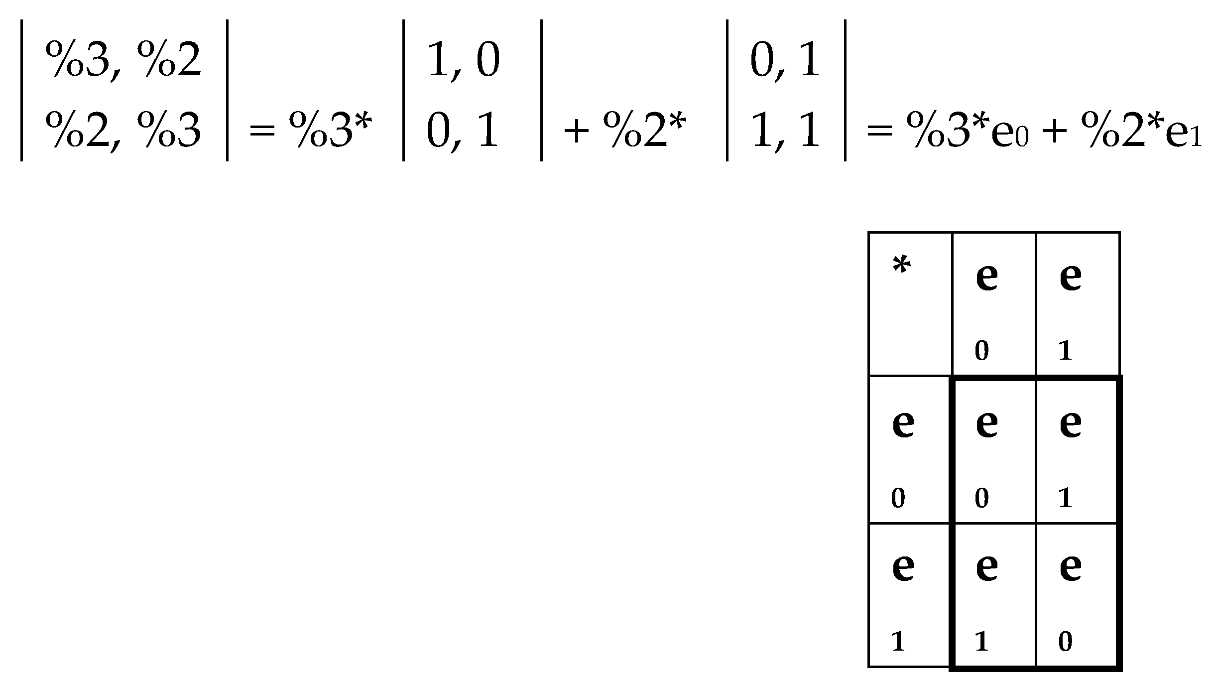
Figure 19 shows that the first matrix C₀₆ is decomposed into two matrices e₀ and e₁, whose set is closed relative to multiplication and defines the multiplication table of the 2-dimensional algebra of hyperbolic (or double) numbers z = x + y j, where x and y are real numbers, j² = 1, and j ≠ ±1 [Kantor, Solodovnikov, 1989]. The multiplication table of bases elements of this algebra is shown in Figure 19, at right.

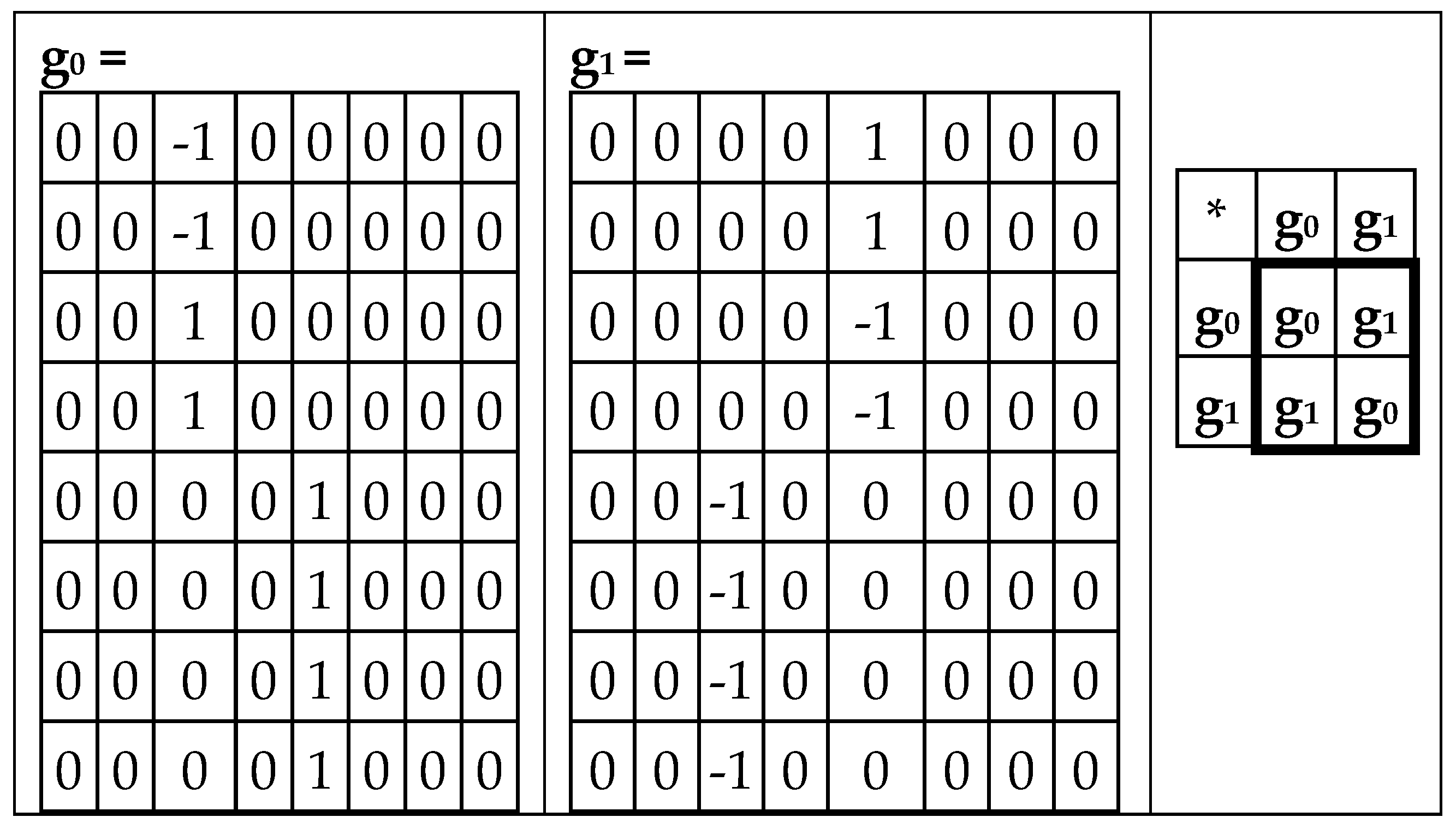
Figure 20 shows that the second matrix C₂₄ (from Figure 18) is decomposed into the sum of two matrices g₀ and g₁, whose set is also closed relative to multiplication and defines the same multiplication table of 2-dimensional algebra of hyperbolic numbers.

Now let us turn to the odd-columns matrix in Figure 3, at bottom right. It is the sum of two matrices shown in Figure 24, at bottom. The first matrix contains only two non-zero columns, which are numerated by root-complementary binary numbers 001 and 111 (that is, numbers 1 and 7 in decimal notation) and is denoted K₁₇. The second matrix contains only two non-zero columns, which are numerated by root-complementary binary numbers 011 and 101 (that is, numbers 3 and 5 in decimal notation) and is denoted K₃₅.

Figure 21. The decomposition of the odd-columns matrix from Figure 3 (at bottom right) into the sum of matrices K₁₇ (at left) and K₃₅ (at right). Empty cells contain zeros. The matrices at the bottom present numbers of columns in decimal notation.

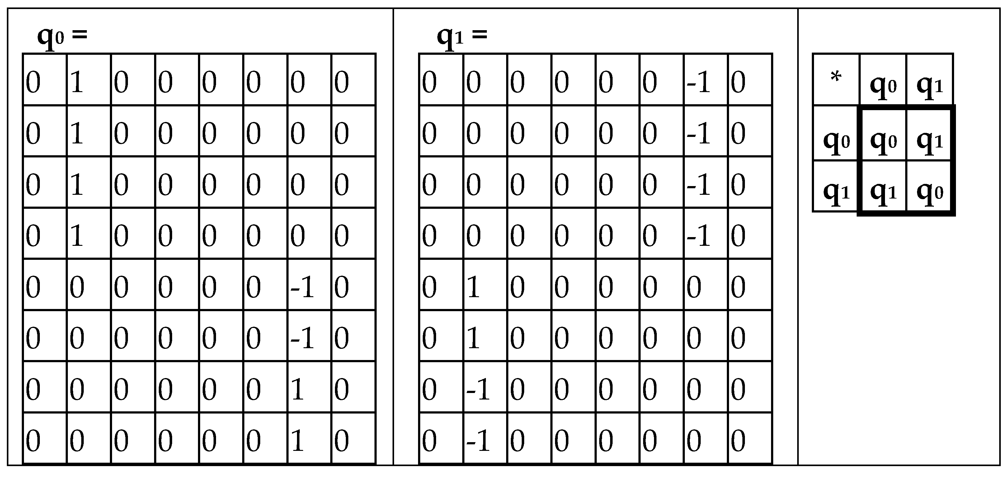
Figure 22 shows that the first matrix K₁₇ is decomposed into the sum of two matrices q₀ and q₁, whose set is closed relative to multiplication and defines the multiplication table of the 2-dimensional algebra of hyperbolic numbers.

Figure 23 shows that the second matrix K₃₅ (from Figure 21) is decomposed into the sum of two matrices h₀ and h₁, whose set is closed relative to multiplication and defines the same multiplication table of the 2-dimensional algebra of hyperbolic numbers.

These results about the connection between the algebra of hyperbolic numbers and the root-complementary relations in the structural set of triplets are especial interesting if one takes into account many other data about the role of hyperbolic numbers in genetics [Petoukhov, 2020a,b, 2021a]. Below in this article the topic of hyperbolic numbers is continued in connection with new universal rules of stochastic organization of genomic DNAs of eukaryotes and prokaryotes.

7. Universal algorithms for dichotomies of probabilities in hydrogen bond sequences of genomic DNAs

A lot of new data on the important significance of the principle “like begets like” and related binary oppositions in the genetic system is found in the study of information sequences of genomic DNA. We will talk about the universal algorithms of dichotomies of probabilities discovered by the author in binary representations of these sequences.

The results described below on universal rules of dichotomies of n-plet probabilities and on corresponding fractal trees of percentages in genomic DNAs have been obtained by the author on a significant number of DNAs of many eukaryotic and prokaryotic genomes, including the following:

all 24 human chromosomes;
all chromosomes of drosophila, mouse, worm, many plants;
19 genomes of bacteria and archaea;
many extremophiles, living in extreme conditions, for example, radiation with a level 1000 times higher than fatal for humans.

One can mention that these genomic DNAs were early analyzed by the author concerning another theme related to the hyperbolic rules of amounts of nucleotide n-plets in genomic DNAs [Petoukhov, 2020c]. This article illustrates these general results and rules with examples of percentage data related to DNAs of human chromosome №1, the plant Arabidopsis thaliana, and bacteria Bradyrhizobium japonicum.

Let’s start the presentation of the obtained results with the analysis of the hydrogen bond sequence (or briefly H-sequence) in DNA of human chromosome №1. This DNA contains about 250 million of nucleotides A, T, C, and G and correspondingly the same amount of the complementary hydrogen bonds 2 and 3 (initial data on this chromosome were taken from the GenBank: https://www.ncbi.nlm.nih.gov/nuccore/NC_000001.11).

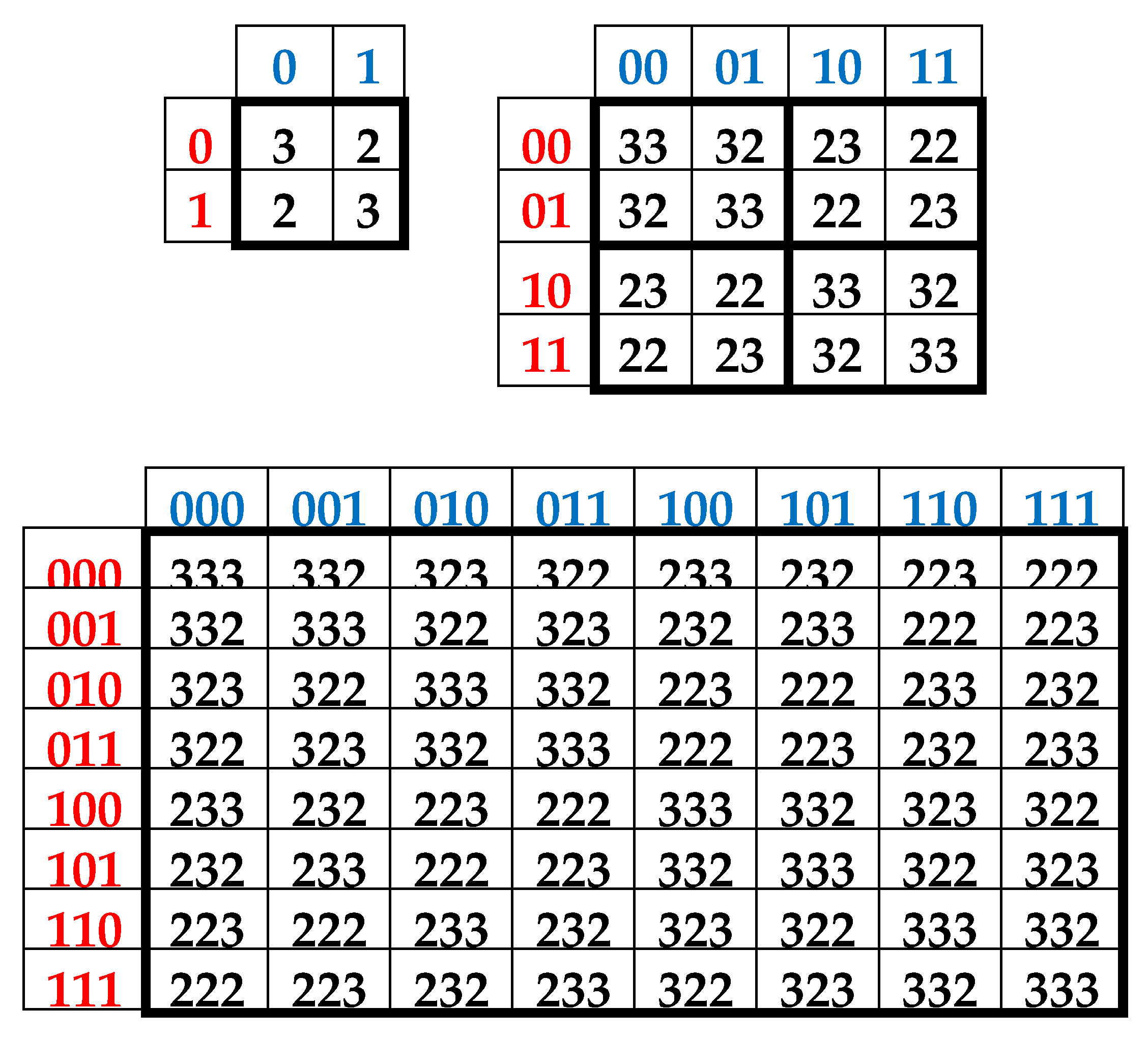
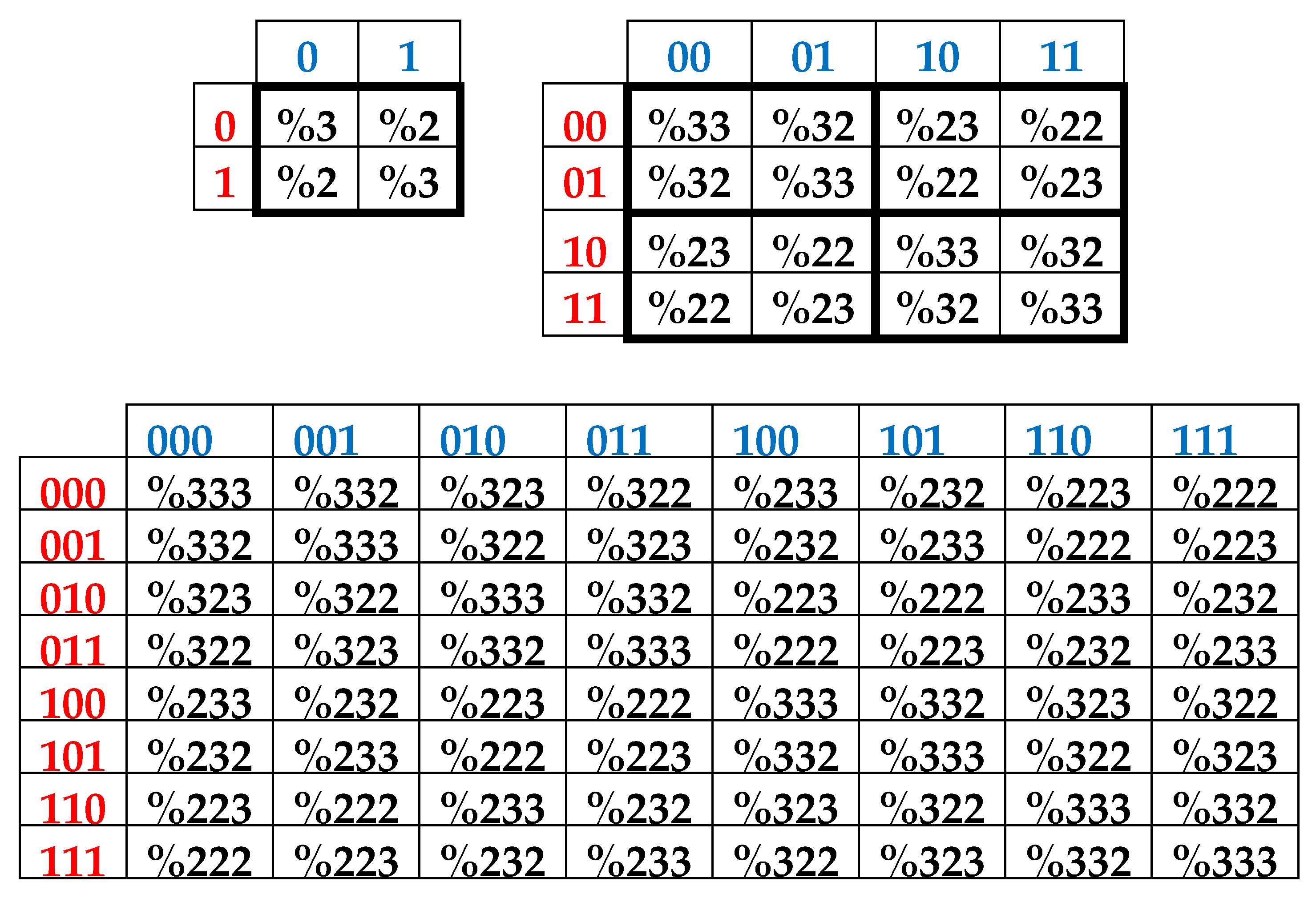
In the author’s approach, the H-sequence of this chromosomal DNA is firstly presented as a H-monoplets sequence where percentages %2 and %3 of each of 2 possible kinds of members (that is, digits 2 and 3) are computer calculated.

Secondly, the H-sequence of this DNA is presented as a H-duplets sequence where percentages %22, %23, %32, and %33 of each of 4 possible kinds of H-duplets (that is, 22, 23, 32, and 33) are computer calculated.

Thirdly, the H-sequence of this DNA is presented as a H-triplets sequence where percentages %222, %223, %232, %233, %322, %323, %332, %333 of each of 8 possible kinds of H-triplets are computer calculated.

Fourth, the H-sequence of this DNA is presented as a H-tetraplets sequence where percentages %2222, %2223, ….., %3333 of each of 16 possible kinds of H-tetraplets are computer calculated.

Fifth, the H-sequence of this DNA is presented as a H-pentaplets sequence where percentages %22222, %22223, …., %33333 of each of 32 kinds of H-pentaplets are computer calculated.

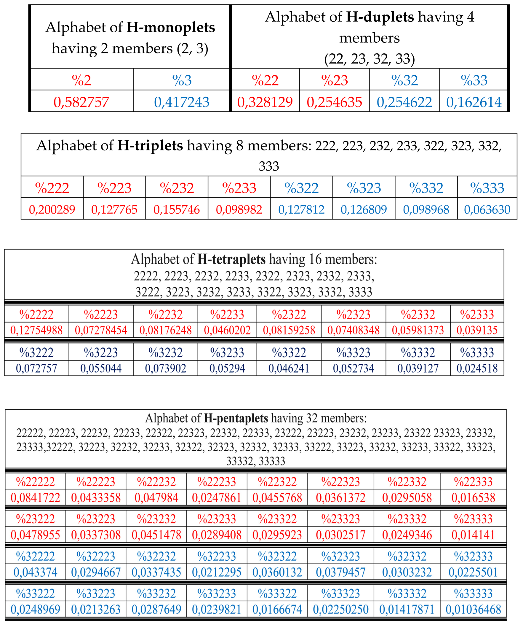
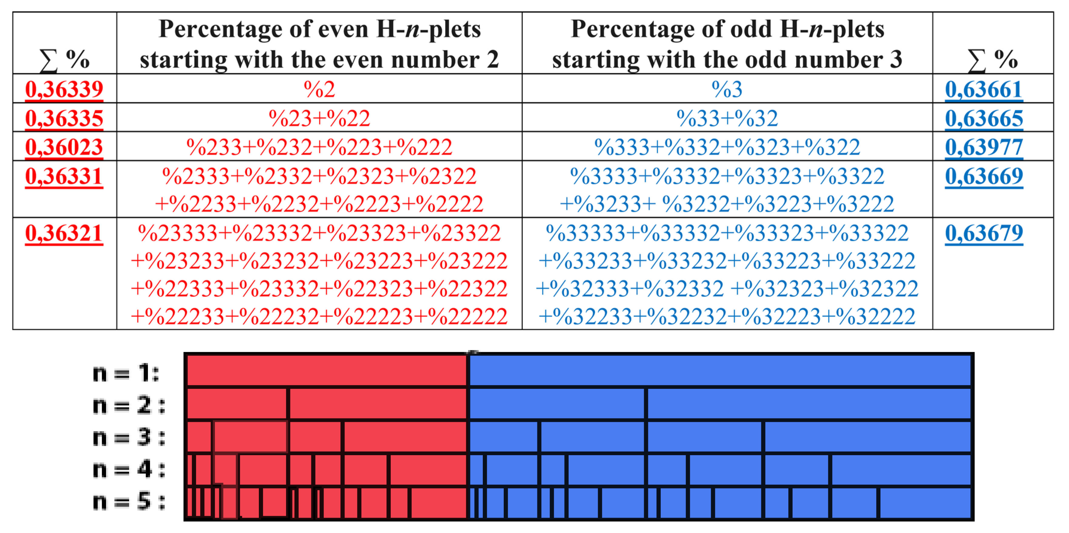
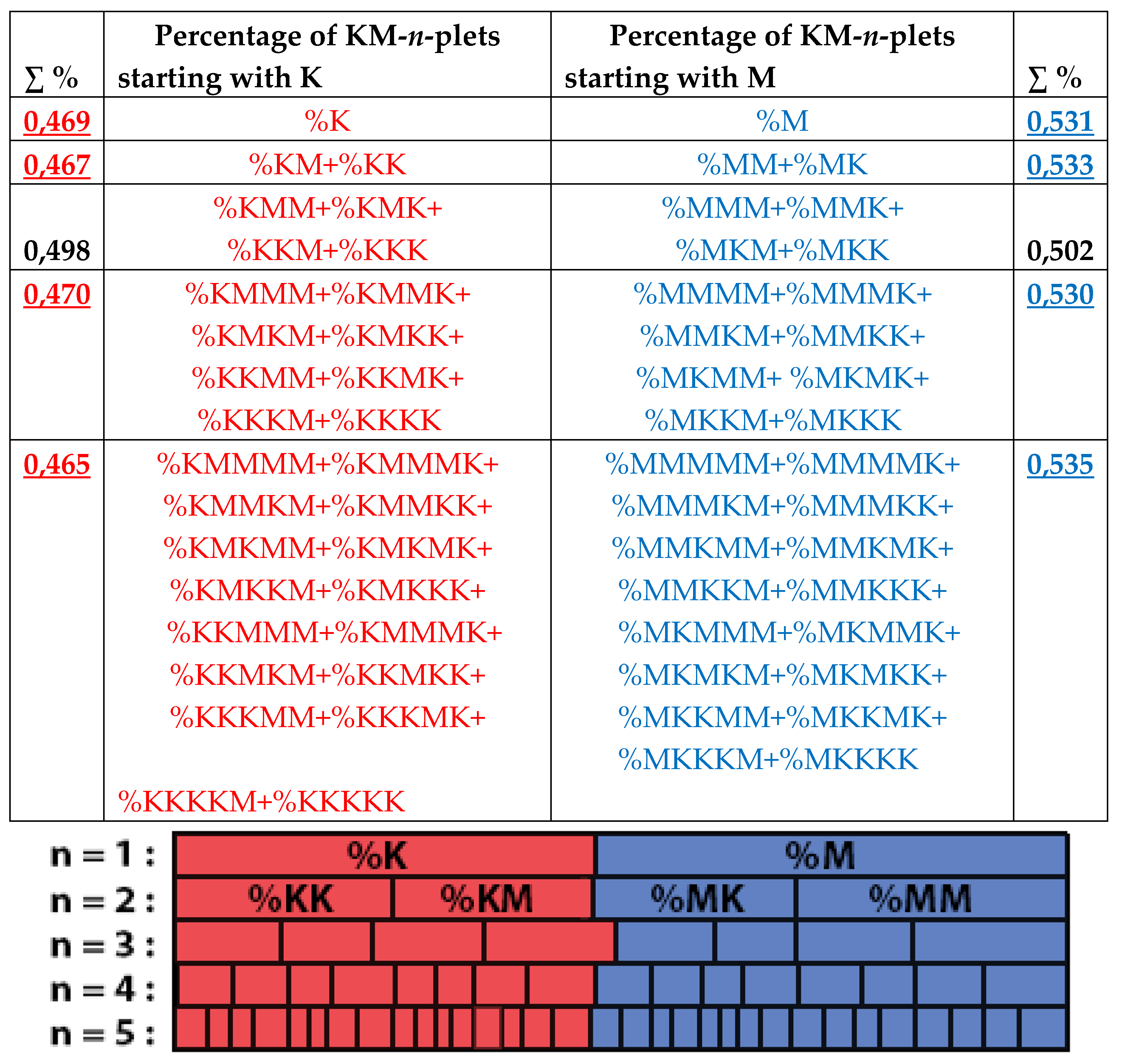
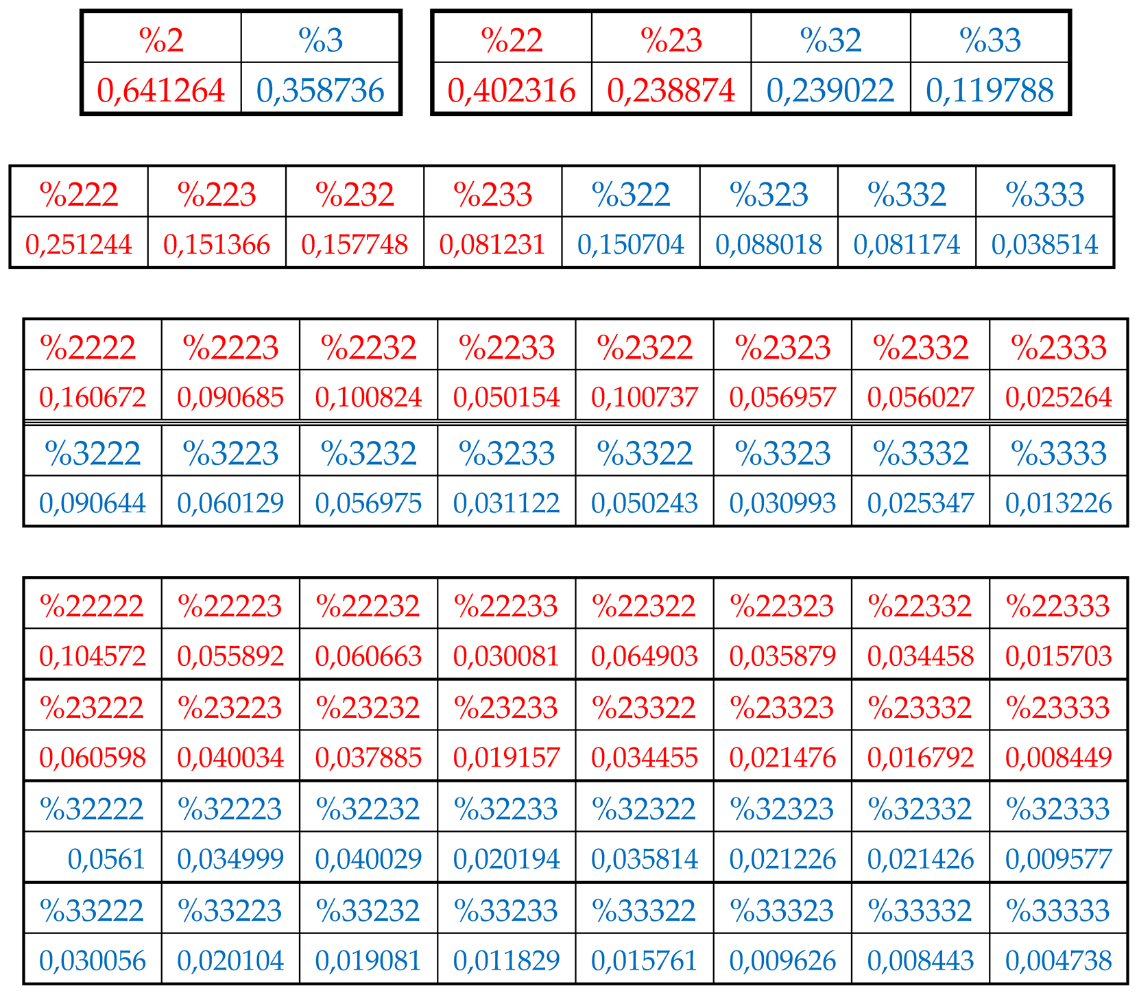
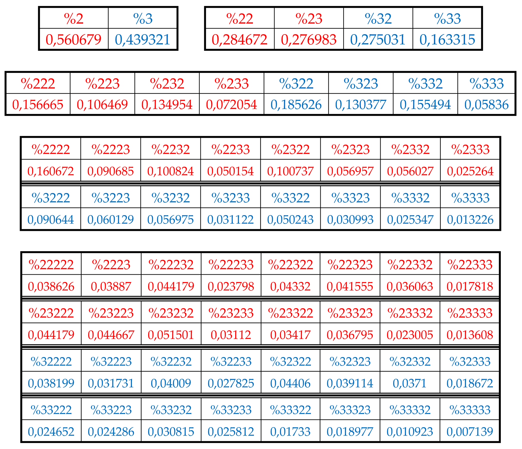
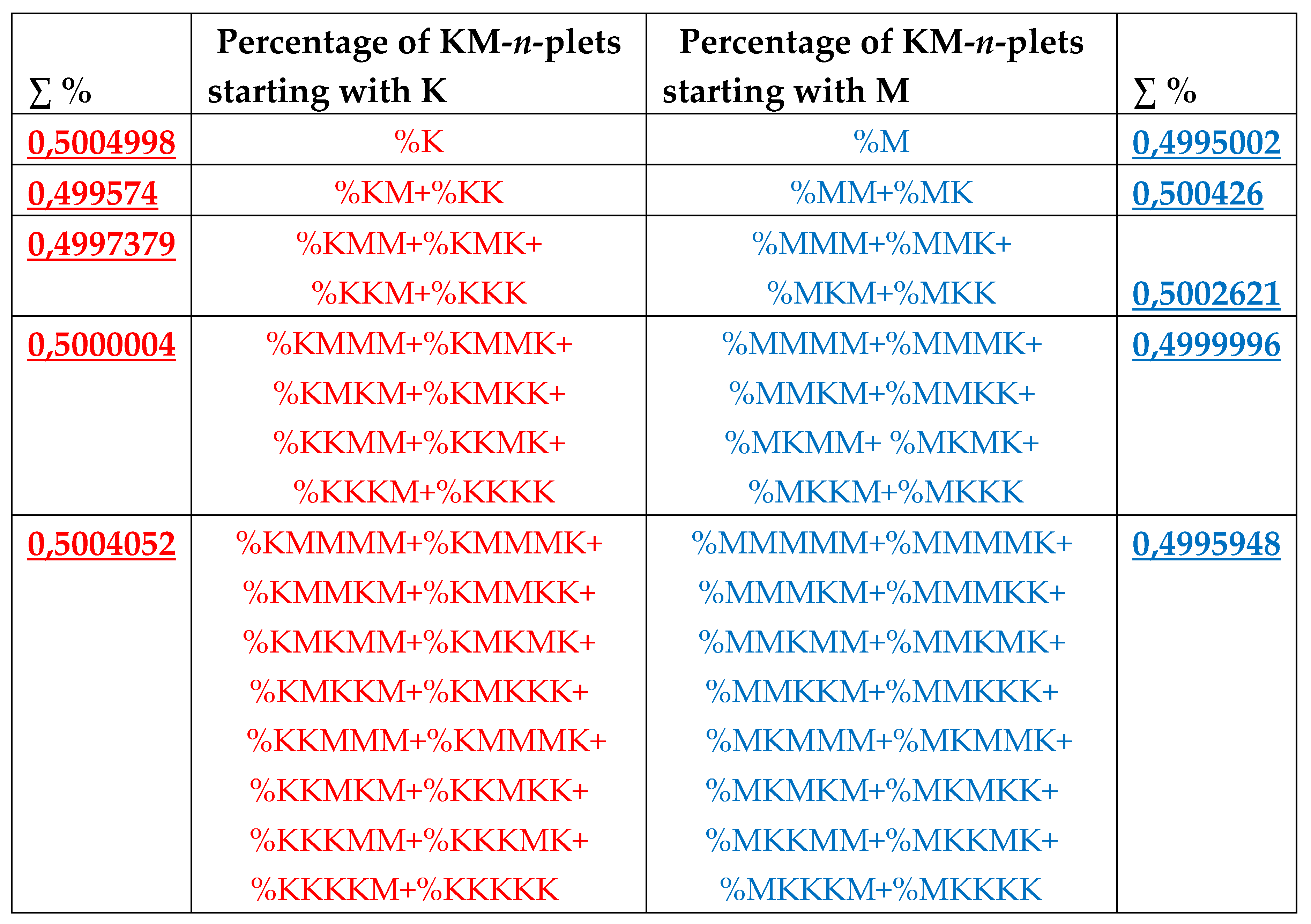
Results of these calculations are presented in Table 1. This author’s method of analysis of percent contents in binary sequences represented as multi-layer sets of n-plets is called “the method of hierarchy binary stochastics” (or, briefly, the HBS-method). The percentage values here and below are given in fractions of a unit.

Table 1. Phenomenological percent values of each of the H-n-plets in corresponding H-n-plets representations of the DNA of human chromosome № 1 (n = 1, 2, 3, 4, 5). Its H-sequence contains about 250 million digits 2 and 3. Initial data on this chromosome were taken from the GenBank: https://www.ncbi.nlm.nih.gov/nuccore/NC_000001.11. Even H-n-plets starting with an even number 2 are in red, and odd H-n-plets starting with an odd number 3 are in blue.

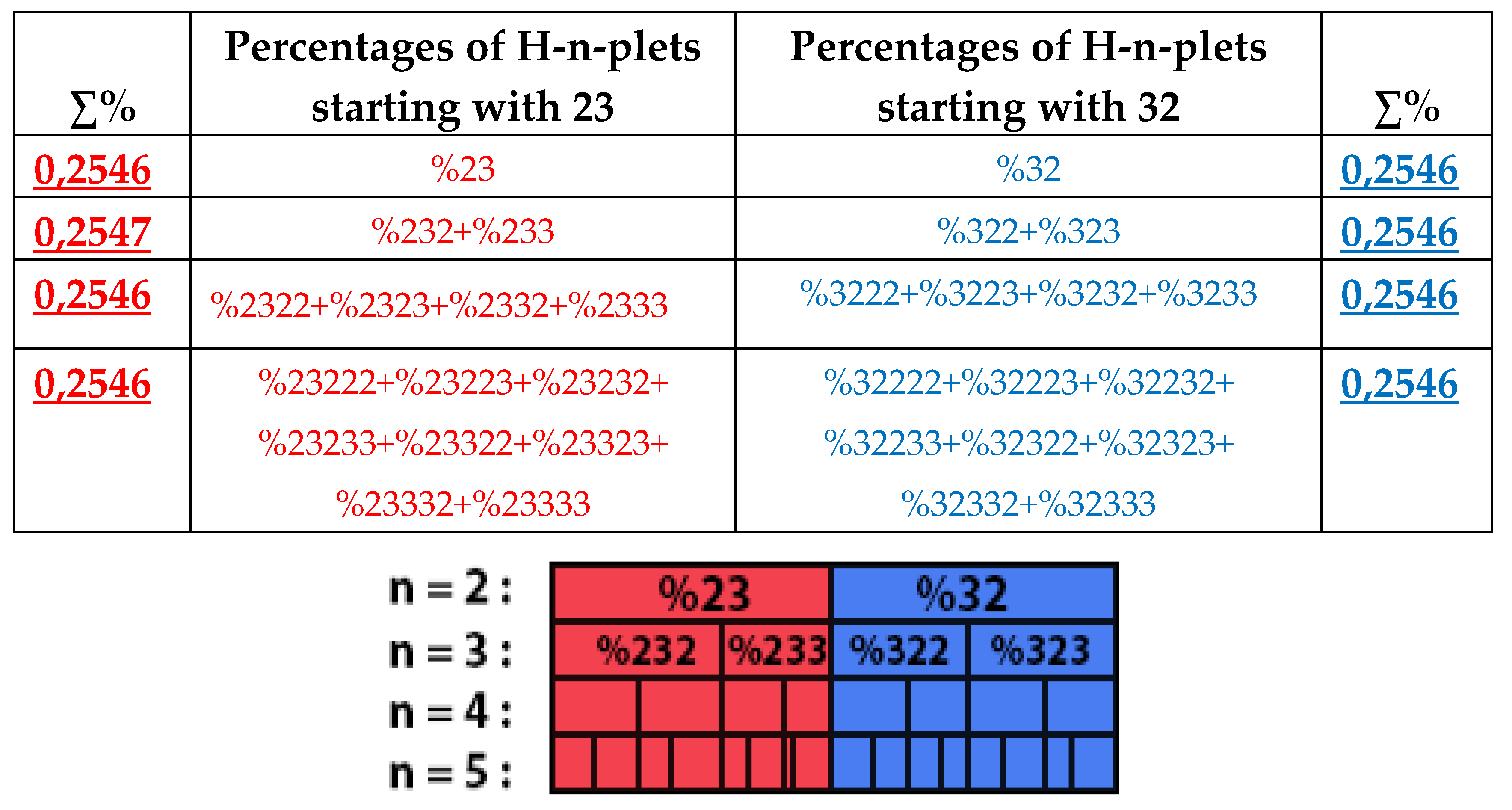
At first glance, these sets of phenomenological percentages of different H-n-plets, which differ in the number of members in the sets and in the size of individual members, are not related to each other. But all these different sets of percentages (or probabilities) of H-n-plets are unexpectedly closely and algorithmically interconnected each with other as any reader can check by using the phenomenological data in Table 1. Below these revealed interconnections are presented in detail. This article shows these regular numeric interconnections by separate examples of analysis of DNAs in the human chromosome № 1, the genome of the plant Arabidopsis thaliana, and the bacteria Bradyrhizobium japonicum.

7.1. Suffix dichotomies of percentages of H-n-plets in DNA of human chromosome № 1.

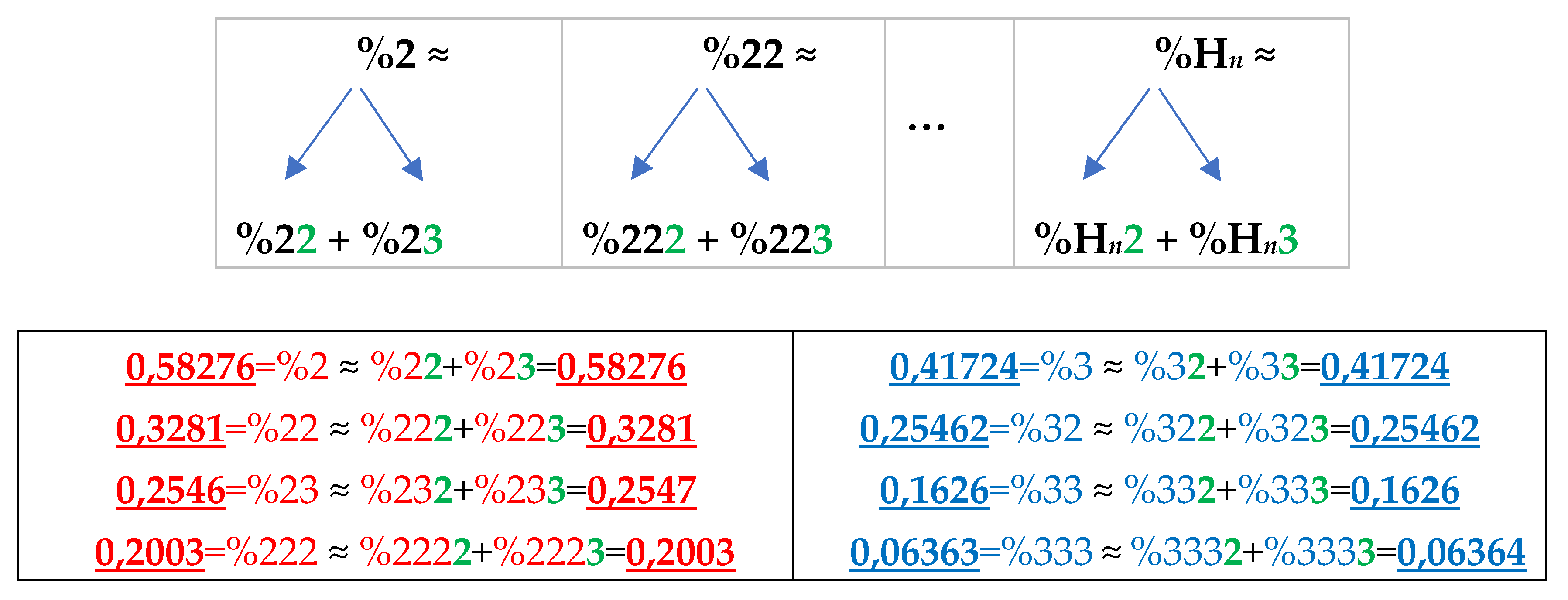
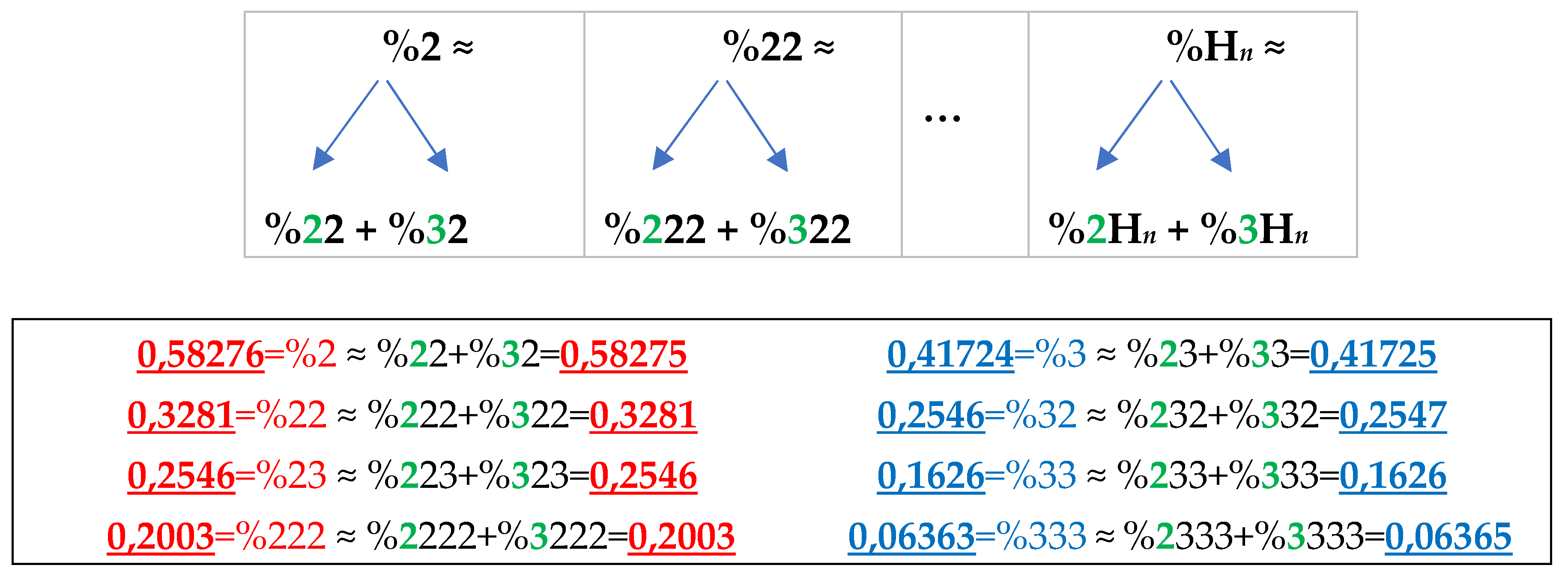
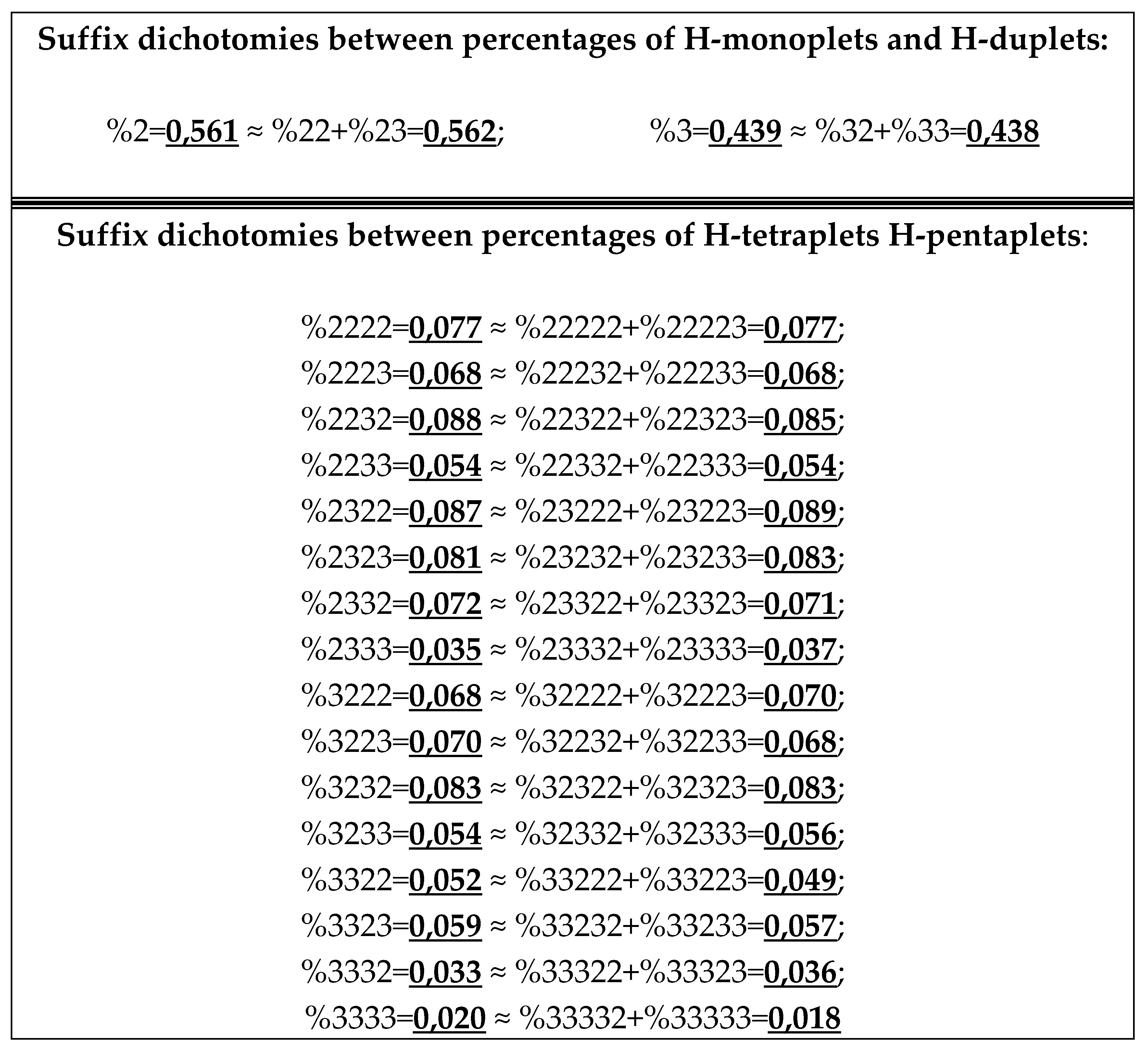
Analysis of the phenomenological data in Table 1 reveals the following: the percentage of any H-n-plet is practically equal to the sum of percentages of those two H-(n+1)-plets, which are generated from this H-n-plet by addition to it the suffixes 2 and 3 as Figure 24 illustrates. We call this type of dichotomy a suffix dichotomy.

Figure 24. At the top: the illustration of the general algorithm of the suffix dichotomy in interrelations between percentages of H-n-plets and H-(n+1)-plets in a genomic binary sequence of hydrogen bonds, which is analyzed by the HBS-method. Here the symbol %H_n denotes a percentage of any H-n-plet under studying (values n = 1, 2, 3, 4, 5 were studied). At the bottom: for the case of DNA of the human chromosome №1, a few numeric examples are shown of high-precision equalities between a percentage of any H-n-plet and a sum of the percentages of two H-(n+1)-plets, which are generated from it by the addition of suffixes 2 and 3. Added suffixes 2 and 3 are highlighted by green. Rounded values of percentages of the H-n-plets are taken from Table 1.

In phenomenological equalities of this type (Figure 24), based on the suffix dichotomy of percentages of H-n-plets, their high accuracy is impressive - up to several decimal places. Figure 24 represents only a few examples of high-precision equality of the percentages. Using numeric data from Table 1, any reader can check himself that such equalities of percentage dichotomies also hold with similar high precisions for all other possible variants of the noted percentages dichotomy, for example, %223≈%2232+%2233, %232 ≈ %2322+%2323, %3332 ≈ %33322+%33323, etc. The author has systematically checked these percentage dichotomic equalities in many genomic DNAs, listed below, only for n = 1, 2, 3, 4, 5. He also selectively checked the fulfillment of such equalities for higher values of n getting positive results in every case, but he did not check at what values of n these dichotomic percentage equalities cease to hold.

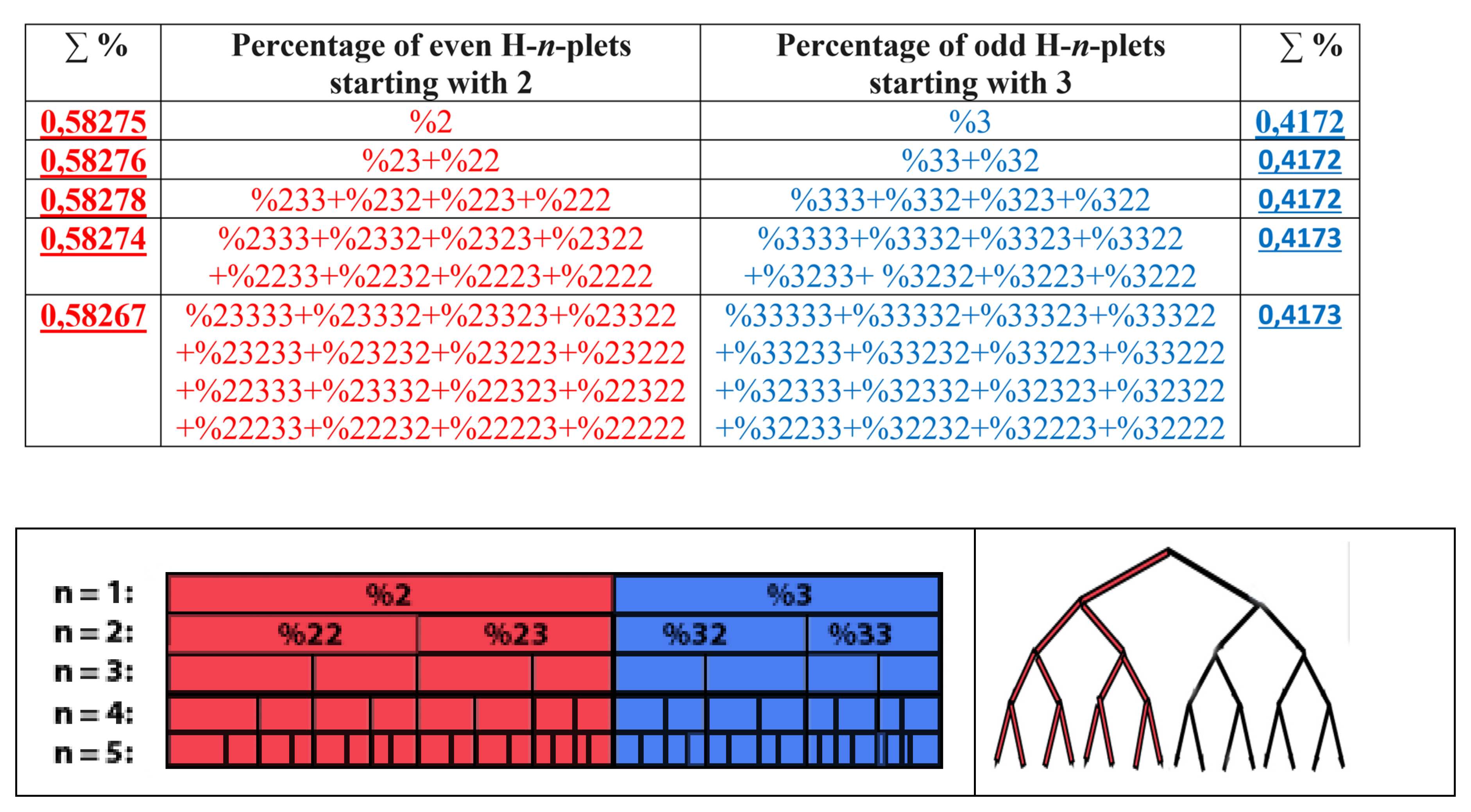
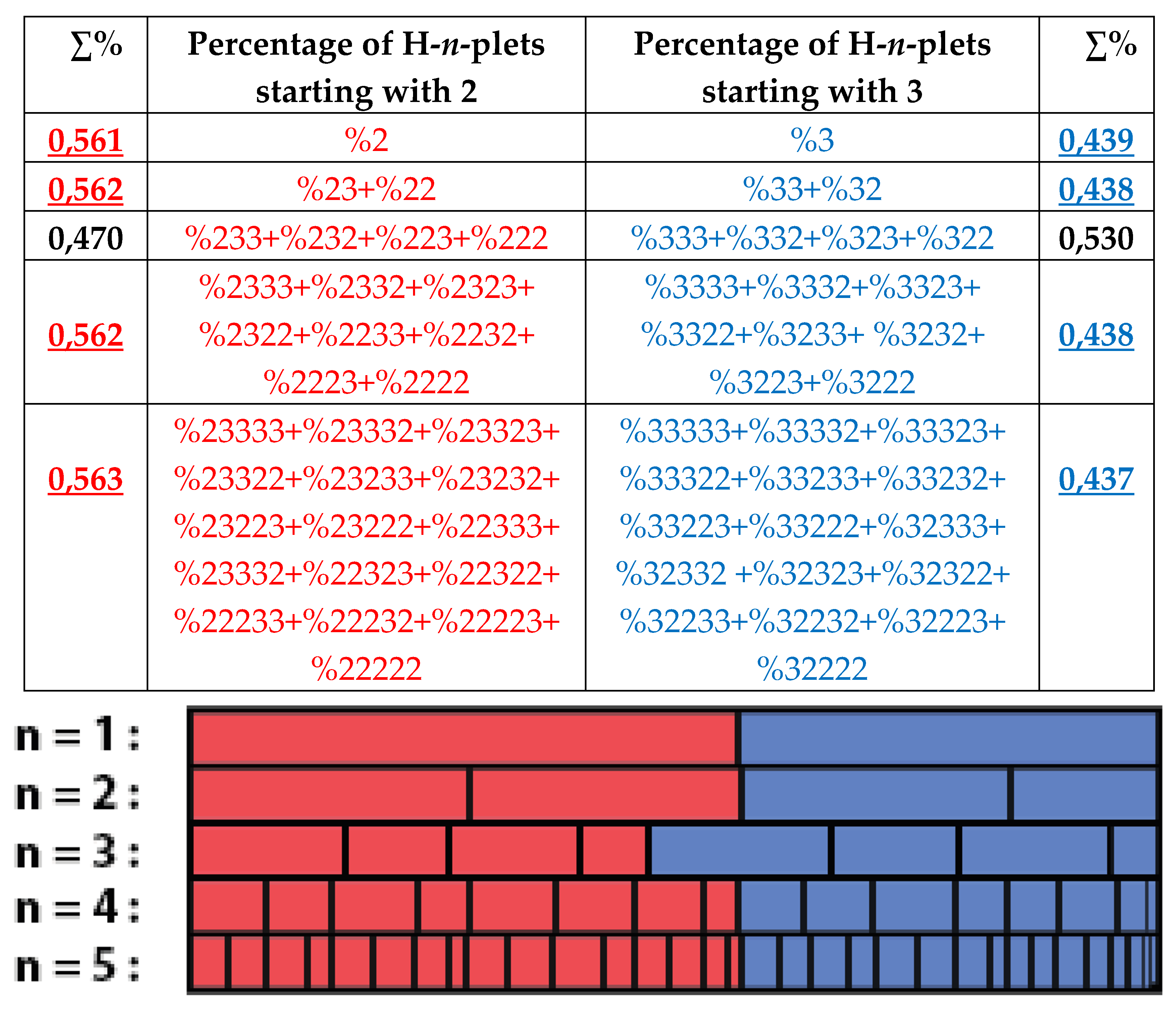
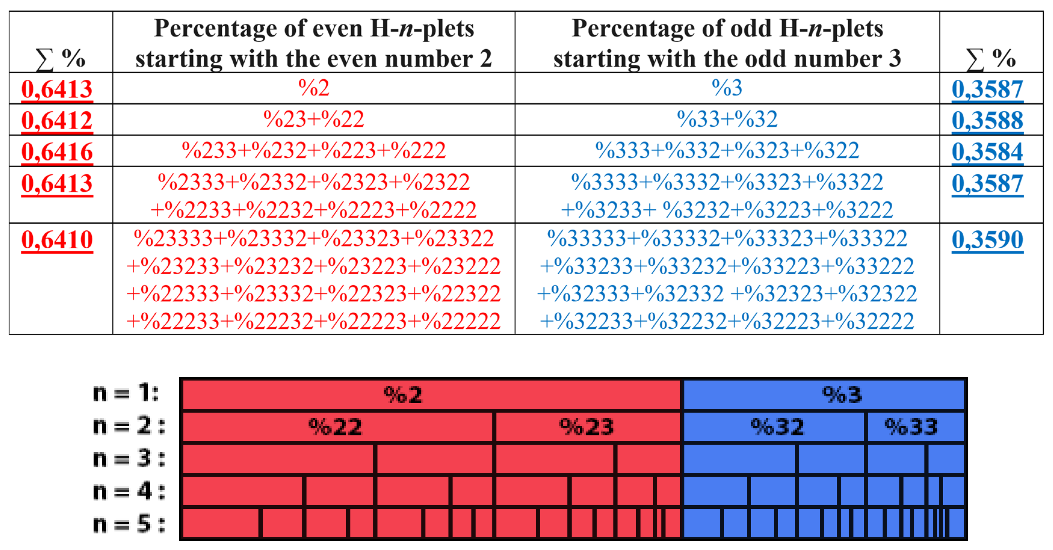
The rule of the suffix dichotomy of H-n-plets percentages leads to fractal dichotomous trees of H-n-plets percentages, which is shown in Figure 25 for the case of DNA of human chromosome № 1. H-n-plets starting with even digit 2 are conditionally called even H-n-plets (their percentages are marked by pink in Figure 25 and further), and H-n-plets starting with odd digit 3 are called odd H-n-plets (their percentage are marked by blue in Figure 25 and further). Each of the levels of these fractal trees with percentage values of even and odd H-n-plets corresponds to a certain magnitude of n.

Levels of the trees of percentages in Figure 25 contain different quantity of percentage summands, but their sums remain the same with high precision at all the levels: in the tree of even H-n-plets, the sums of percentages of even H-n-plets are equal to 0.5827

\div

0.5828, and in the tree of odd H-n-plets, the sums of percentages of odd H-n-plets are equal to 0,4172

\div

0,4173. These summary values on the different levels are equal to the percentages of H-monoplets: %2 and %3.

In the considered sequences of H-n-plets, numbers 2 and 3 can be denoted with binary numbers 0 and 1 correspondingly. In this case, we get the following transformation:

-: the H-duplets 22, 23, 32, 33 become binary duplets 00, 01, 10, 11 forming the 2-bit dyadic group (they correspond to decimal numbers 0, 1, 2, 3);
-: the H-triplets 222, 223, 232, 233, 322, 323, 332, 333 forming the 3-bit dyadic group (they correspond to decimal numbers 0, 1, 2, 3, 4, 5, 6, 7);
-: the H-tetraplets 2222, 2223, 2233, …, 3333 forming the 4-bit dyadic group (they correspond to decimal numbers 0, 1, 2, 3, …, 14, 15);
-: the H-pentaplets 22222, 22223, 22232, …, 33332, 33333 forming the 5-bit dyadic group (they correspond to decimal numbers 0, 1, 2, 3, …, 30, 31).

One can see in Figure 25 (at the bottom) that, for example, the level with n=5 contains a set of very different percentages of 32 H-pentaplets. It has a quasi-stochastic character, but in this seeming stochastically set, the regular phenomenon of percentage dichotomies exists related to the known principle of even-odd numbers, which was already met above. More precisely, the corresponding rule of percentage dichotomies in the interrelation between the considered levels of H-n-plets is the following:

-: the sum of the percentages of those two n-plets, whose binary numberings are almost identical and differ from one another only by suffixes 0 or 1, is practically equal to the percentage of that (n-1)-plet whose binary numbering is obtained from the named numberings by deleting these suffixes. For example, %1010+%1011 ≈ %101.

This rule of percentage dichotomies is universal and holds for all genomic DNAs studied by the author. For instance, in DNA of human chromosome № 1, we have from the data of Tables 1 the following example of interrelation between representatives of alphabets of 16 H-tetraplets and 8 H-triplets (5):

%101=0,12681 ≈ %1010+%1011=0,07390+0,05294 = 0.12684

(5)

This rule concerns pairs of neighboring binary numberings, one of which is even (its ends digit is 0) and another is odd (it ends digit is 1). It resembles Yin-Yang pairs.

Figure 26 shows the schematic tree of percent dichotomies for H-n-plets who’s sets are presented in a form of dyadic groups of n-bit binary numberings, which present percentages of n-plets of hydrogen bonds 2 and 3 in the genomic DNAs. Each of the dyadic groups is posted at a separate level with the corresponding value n. Figure 25 and Figure 26 present in the graphical form the important phenomenological fact of existence of a structural non-stochastic module (or a non-stochastic unit) of probabilities in stochastic organization of genomic DNAs as a set of n-plets layers. This universal non-stochastic module of probabilities, which is based on a deterministic condition, is a pair of percentages of the mentioned n-plets with even and odd binary numberings: in different pairs of percentages of two n-plets with such even and odd numberings, a percent value of one n-plet of this pair can be unpredictable and stochastic but the sum of percent values of both such n-plets are always practically equal to a percent value of the (n-1)-plet, having the same binary representation with the exception of the deleted last binary digit (see Figure 26). For the artistic representation of such non-stochastic modules of probabilities, as the sums of the percentages of two corresponding n-plets having even-odd numberings, one can use the well-known Yin-Yang symbol ☯, which was the personal coat of arms of Niels Bohr

The above can also be formulated as the principle of interconnections of probabilities in n-textual representations of genomic DNAs (6):

%(n)0 + %(n)1 ≈ %(n)

(6)

where symbols (n)0 and (n)1 denote two neighboring (n+1)-plets having their suffixes 0 and 1, and the symbol %(n) denotes a corresponding n-plet with the same binary numbering but without these suffixes.

For the artistic representation of such non-stochastic modules of probabilities, as the sums of the percentages of two corresponding n-plets having even-odd numberings, one can use the well-known Yin-Yang symbol ☯, which was the personal coat of arms of Niels Bohr.

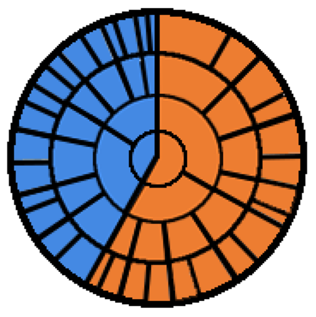
Such percentage trees and complete sets of percentages of n-plets in binary sequences can be also graphically represented in a circular form with multi-level mandala-like images whose example is shown in Figure 27.

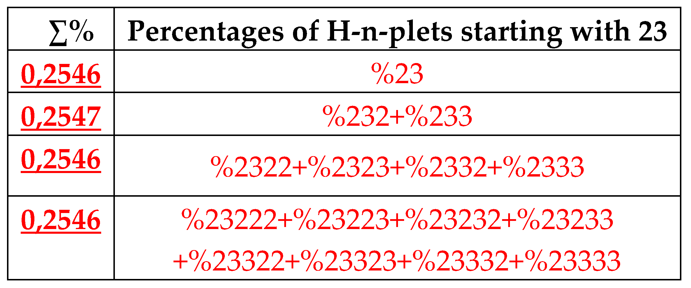
The dichotomic percentage trees in Figure 25 are called fractal (or fractal-like) since each of their numeric member (that is, a percent value of any H-n-plet) is a top of its own dichotomic tree of percent values of H-n-plets from the genomic DNA. Any reader can check this statement using percentage data from Table 1. Figure 28 demonstrates this for the particular case of %23 as the top of its own dichotomic fractal tree.

7.1.1. The rule of percentage equalities in the set of genomic H-n-plets

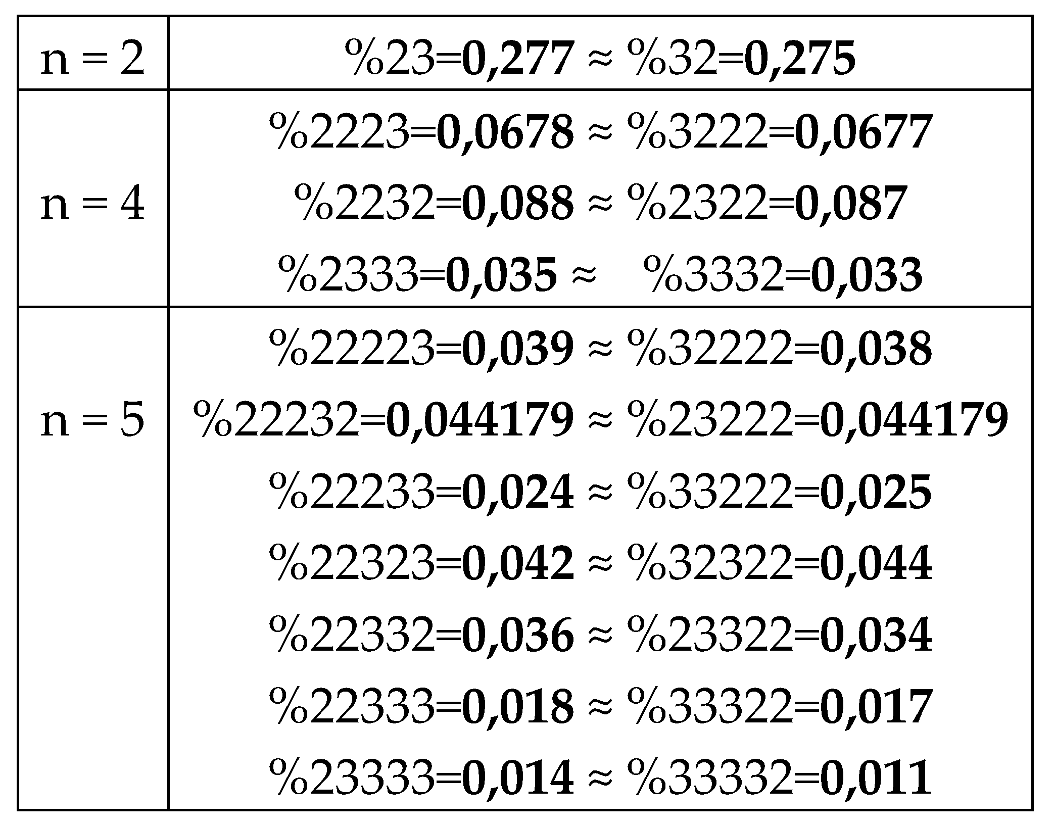
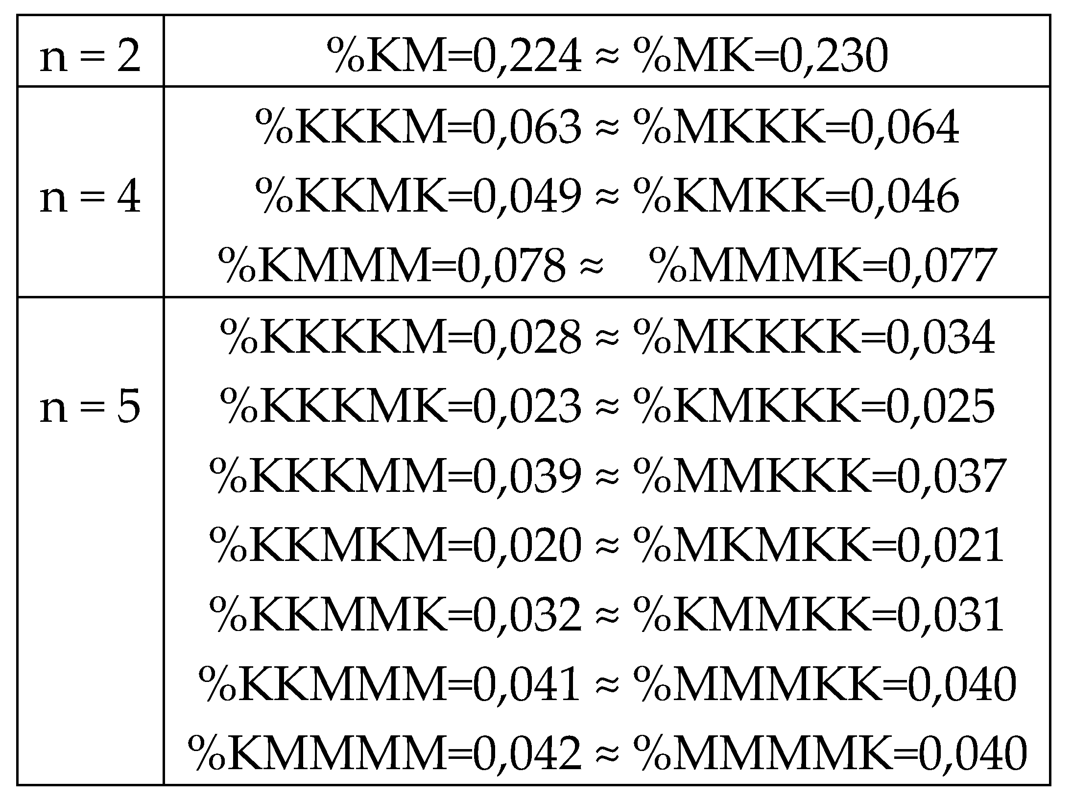
The numeric data in Table 1 confirm else the following phenomenological rule: those two H-n-plets, which are read as mirror (or reversed) copies of each another (such as 223 and 322), always have almost the same percent values in the genomic H-n-plet sequence. This rule of practical equalities of percent values of such n-plets further reduces the degree of stochasticity in the organization of H-n-plet sequences in genomic DNAs. To demonstrate examples of this rule, we write out all such pairs of reversed H-n-plets from Table 1 (percentages are rounded):

%23=%32=0,2546; %223=%322=0,1278; %233=%332=0,0990;

%2223=%3222=0,0728; %2232=%2322=0,082; %2233=%3322=0,046;

%2333=%3332=0,0391; %2323=%3232=0,074; %3233=%3323=0,053;

%22223=%32222=0,043; %22232=%23222=0,048; %22233=%33222=0,025;

%22323=%32322=0,036; %22332=%23322=0,0296; %22333=%33322=0,017;

%23223=%32232=0,0337; %23233=%33232=0,029; %23323=%32332=0,0303;

%23333=%33332=0,014; %32233=%33223=0,0213; %32333=%33323=0,023

(7)

Even and odd fractal trees in Figure 25 are asymmetric each to another: at all the levels, sums of percentages of even H-n-plets are not equal to sums of percentages of odd H-n-plets. But is it possible to algorithmically build fractal trees with symmetrical left and right halves based on the phenomenological data on the percentage of H-n-plets from Table 1? Yes, you can. To construct such symmetric percentage trees, it suffices to take as their vertices the percentages of those two H-n-plets that are read as mirror (or reversed) copies of each other (for example, %23 and %32, or %223 and %322); then the algorithm of the suffix dichotomies is applied for these vertices to construct sets of H-n-plets at other levels of the trees. Figure 29 shows an example of so constructing symmetric fractal trees where percentage sums of even and odd H-n-plets are practically identical at all their levels.

One should note that for genomic DNAs, the rule of practical equality between percentages of those n-plets, which are read as mirror copies of each another, holds not only for the case of H-n-plets but also for cases of binary sequences of purine-pyrimidine n-plets and keto-amino n-plets, which are considered in this article below.

7.2. Prefix dichotomies of percentages of H-n-plets in DNA of human chromosome № 1

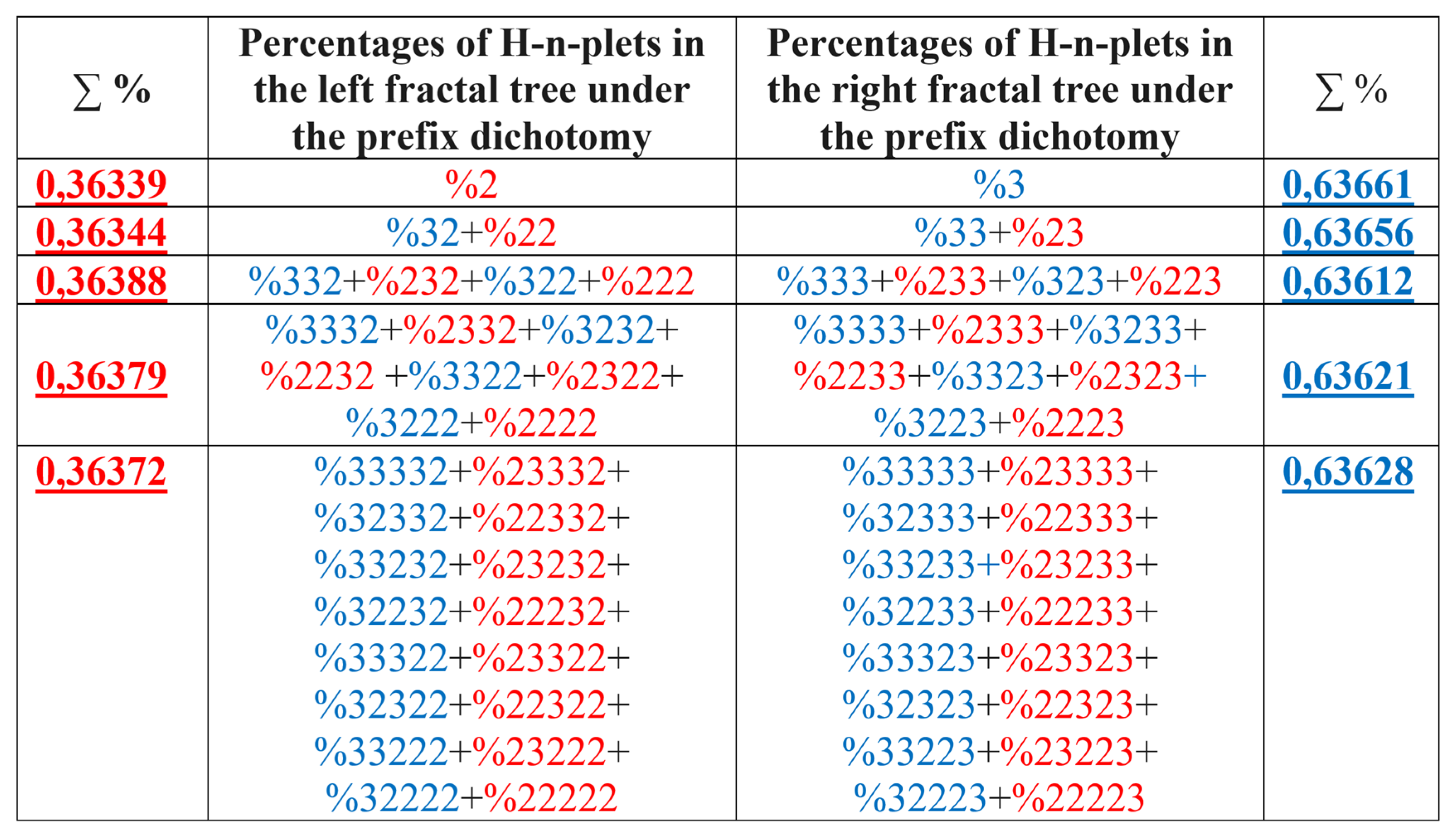
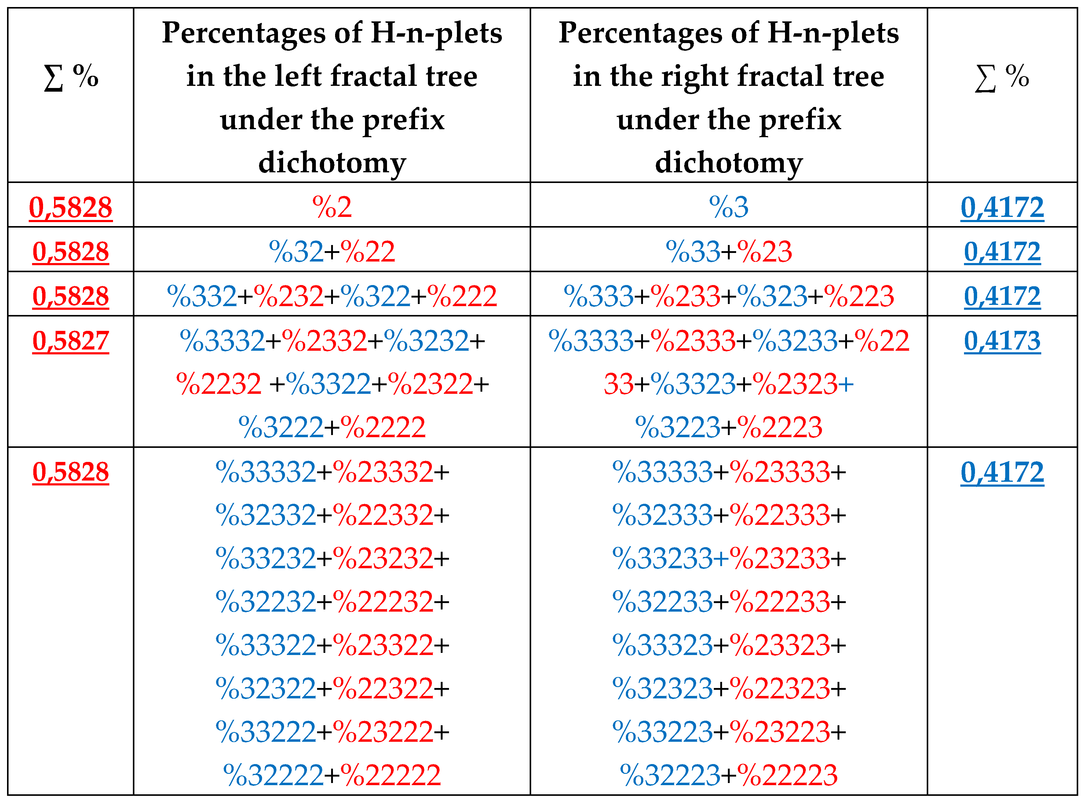
Analysis of the phenomenological data in Table 1 also reveals that besides the described algorithm of suffix dichotomies, there exists an algorithm of prefix dichotomies in the genomic DNA: the percentage of any H-n-plet is practically equal to the sum of percentages of those two H-(n+1)-plets, which are generated from this H-n-plet by addition to it the prefixes 2 and 3 as Figure 30 illustrates. We call this type of dichotomy the prefix dichotomy.

The algorithm of the prefix dichotomy of percentages of genomic H-n-plets generates corresponding fractal trees of percentages illustrated in Figure 31. The lists of H-n-plets in these left and right fractal trees differ from the lists of H-n-plets in the trees of even and odd H-n-plets in Figure 25. But the rule of approximate equalities of percentages sums at all the levels of each tree holds in this case as well.

It should be noted that, in a general case, percentage value of each H-n-plet simultaneously belongs to different fractal trees of percentages of H-n-plets. For example, %232 belongs to all above-described fractal trees. The stochastic organization of hydrogen bond sequences in genomic DNAs deals with interrelated nets of fractal dichotomic trees.

As it was above noted, the author has obtained a confirmation of the described rules of dichotomies of percent values of H-n-plets in analysis of a wide set of genomic DNAs in eukaryotes and prokaryotes without any exception. This testifies in favor of the existence of universal rules of nontrivial algebraic invariants of a globally genomic nature, which remain unchanged over million years of biological evolution, during which millions of species of organisms die off and new ones appear (although locally genomic sequences are modified by mutations, natural selection mechanisms, etc.). At this stage of research, the described rules are a candidacy for the role of universal genetic rules. Additional studies of the widest set of genomic DNAs are required to test their universality.

One should add that in considered binary sequences, digits 2 and 3 of hydrogen bonds can be denoted by binary numbers 0 and 1 to note a connection of the families of H-n-plets, having 2ⁿ-members in each family under fixed value of n, with dyadic groups of binary numbers. In dyadic groups of binary numbers, there exists the above-described notion of complementarity in pairs of binary numbers, which are transformed each to another by the complementarity operation 0↔1.This operation is used in matrix genetics to reveal hidden complementary relations in emergence properties of the genetic coding system (see above paragraphs 2 and 3). Concerning the considered fractal trees of percent dichotomies in Figure 25, Figure 28 and Figure 30, one can note that at each of their levels H-n-plets in left and right trees consists of complementary H-n-plets. For example, in Figure 25 at the level of duplets (n = 2), the left tree contains percentages of H-duplets 22, 23 and the right tree contains percentages of their complementary H-duplets 33 and 32 (the complementarity operation is 2↔3). In this relation, these left and right fractal trees are complementary each to another. Such complementarities also hold for other pairs of dichotomy fractal trees presented below. It is additional evidence in favor of the key role of the principle of complementarity and dichotomies in the genetic system related to the ancient principle “like begets like”. The complementarity principle presented in the DNA double helix model by Watson and Crick is a particular case of its realization in living matter.

7.3. Regarding importance of hydrogen bonds and the binary-stochastic analogy between genetic and nervous systems

The described rules concerning to percentages values of n-plets of hydrogen bonds in genomic DNAs attract an additional attention in the light of the modern knowledge about an important role of hydrogen bonds in genetics and living bodies in the whole. Really, as it is known, the hydrogen bonds are one of the most important components of life. It occurs in many biological structures [American Institute Of Physics, 1999]. In particular, hydrogen bonding play the role of a promotional factor for intermolecular vibrational energy relaxation, and as a driving force for the occurrences of specific reaction channels in binary molecular complexes [Chatterjee, Biswas, Chakraborty, 2020] Hydrogen bonding is an important factor in the functioning of enzymes, which manage molecular processes in biological bodies [Shan, Herschlag, 1999; Trylska, Grochowski, McCammom, 2004]. The ultrafast intermolecular hydrogen bond dynamics of water was revealed [Zhao, et al., 2020]. The Nobel laureate L. Pauling emphasized: “Although the hydrogen bond is not a strong bond, it has a great significance in determining the properties of substances… It has been recognized that hydrogen bonds restrain protein molecules to their native configurations, and I believe that as the methods of structural chemistry are further applied to physiological problems it will be found that the significance of the hydrogen bond for physiology is greater than that of any other single structural feature” [Pauling, 1940].

Hydrogen bonds determine many of the properties of water and ice. Many emergent properties of hydrogen bond systems in living bodies have yet to be discovered. The richness of the emergent properties of hydrogen bond systems can be illustrated by the example of jellyfish, which are 98% water, representing, figuratively speaking, a configured bag with a water substrate of hydrogen bonds. At the same time, jellyfish are the most ancient multicellular animals of the Earth with a huge evolutionary diversity of species and functional capabilities, including the possibility of sexual and asexual reproduction. Jellyfish of some species for reproduction are dichotomically divided in half or are engaged in budding. Finally, there are the jellyfish Turritopsis dohrnii, which have the ability to live forever by reversing the aging process. And jellyfish cannot be attributed to any one group. Many of them are not only on completely different branches of the phylogenetic tree of animals, but also live in different environments: some species prefer the surface of the ocean, others live in the depths, and still others have chosen fresh waters. Let’s add to the topic of hydrogen bonds that hydrogen is the most common element in the Universe: it accounts for about 88.6% of all atoms. The discovery of the above-described universal rules of percent values of n-plets of hydrogen bonds in genomic DNAs gives new abilities and approaches to understanding and modeling the important role of hydrogen bonds in living nature.

Concerning sequences of 2 and 3 hydrogen bonds in DNAs, it is interesting that the generation of electrical spikes in brain neurons is connected with the same numbers 2 and 3. These neuron spikes are produced by using a flow of Na+ and K+ ions, which is provided by so called Na+/K+ pump. But the Na+/K+ pump uses the energy of one ATP molecule to exchange 3 intracellular Na+ ions for 2 extracellular K+ ions [Glitsch, 2001]. Some publications claim that functional features of the Na+/K+ pump can be used for brain computations [Forrest, 2014].

Concerning the above-described universal rule of stochastic organization of genomic DNAs sequences of hydrogen bonds numbers 2 and 3 in genetic information, the following idea arises:

-: the work of the nervous system, including brain work, uses the sequences of numbers 2 and 3 in neural activity by analogy with the use of sequences of numbers 2 and 3 in genetic DNA molecules.

This idea can be called a hypothesis about the numeric binary-stochastic analogy of the work of the nervous and genetic systems. This idea is supported by the following circumstances: 1) the nervous system is genetically inherited, and therefore must be structurally associated with genetic coding and genetic informatics; 2) in biological evolution, the nervous system appeared relatively recently, and many organisms lived and live without it, having efficient information processing systems based on the activity of genetically inherited proteins and enzymes, in which hydrogen bonds play an important role; 3) the work of neurons is also based on stochastics: from different synapses to a neuron, signals arrive in a stochastic manner, which are somehow processed in networks of neurons; 4) the above-described universal rules of dichotomies in percentage interconnections of n-plets of hydrogen bonds 2 and 3 in the multi-textual representation of genomic DNAs are correlated in some degree with the known fact of neurophysiology that “the branching of neuronal axons and dendrites are always bifurcations. That is, they always branch of into two separate paths and never three, four or five etc.” [Tsang, 2016, p. 235].

Speaking on the author’s hypothesis about the numeric binary-stochastic organization of nervous system work, one can additionally remind about another fact of the importance of binary principles in neurons activity: the “all-or-none law” notes that inherited activity of a single nerve fiber under its stimulation always gives a maximal response or none at all [https://en.wikipedia.org/wiki/All-or-none_law]. (The author here expresses special thanks to Prof. Matthew He from the USA, who told him in 2018 on the publication about these numbers 3 and 2 under generating spikes in neurons).

The formulated hypothesis assumes that information in nerve fibers is represented by sequences of ion numbers 2 and 3. To confirm or refute this hypothesis, special experimental studies on neurons are needed.

Concerning the topic of numbers 3 and 2 in genetics, one should note the work [Boulay, 2022, 2023] presenting author’s results about an important role of numbers 3 and 2 in structural organization of the set 20 proteinogenic amino acids in relation to their physicochemical properties, etc.

7.4. Dichotomies of percentages of H-n-plets in DNA of the plant Arabidopsis thaliana

Let us turn now to similar analysis of percentages of hydrogen bond n-plets in DNA of Arabidopsis thaliana chromosome № 1 with the HBS-method. Initial data about this chromosomal DNA, whose length is equal to 30427671 bp, were taken from the GenBank: https://www.ncbi.nlm.nih.gov/genome/4. Table 2 shows corresponding percent values of H-n-plets.

Using these data of Table 2, any reader can check that dichotomic rules of H-n-plets percentages, described above for the human chromosomal DNA, hold as well in the chromosomal DNA of the plant Arabidopsis thaliana having another percent values of its H-n-plets. For example, Figure 32 and Figure 33 show fractal trees in the cases of the suffix dichotomy and the prefix dichotomy of percent values of H-n-plets for the chromosomal DNA of Arabidopsis thaliana.

Again, each of the members of these parental fractal trees of probabilities (for example, %23) serves as a top of its own dichotomous fractal tree by analogy with the example in Figure 28).

7.5. Dichotomies of percentages of H-n-plets in genomic DNA of the bacteria Bradyrhizobium japonicum

Let us consider now an example of DNA from a prokaryotic genome of the rhizobacteria Bradyrhizobium japonicum that is of essential economic importance. Initial genomic data about the rhizobacteria Bradyrhizobium japonicum strain E109, (complete genome, 9224208 bp) were taken from https://www.ncbi.nlm.nih.gov/nuccore/CP010313.1?report=genbank. The length of this sequence is more than 20 times shorter than the length of the sequence of the human chromosome №1. 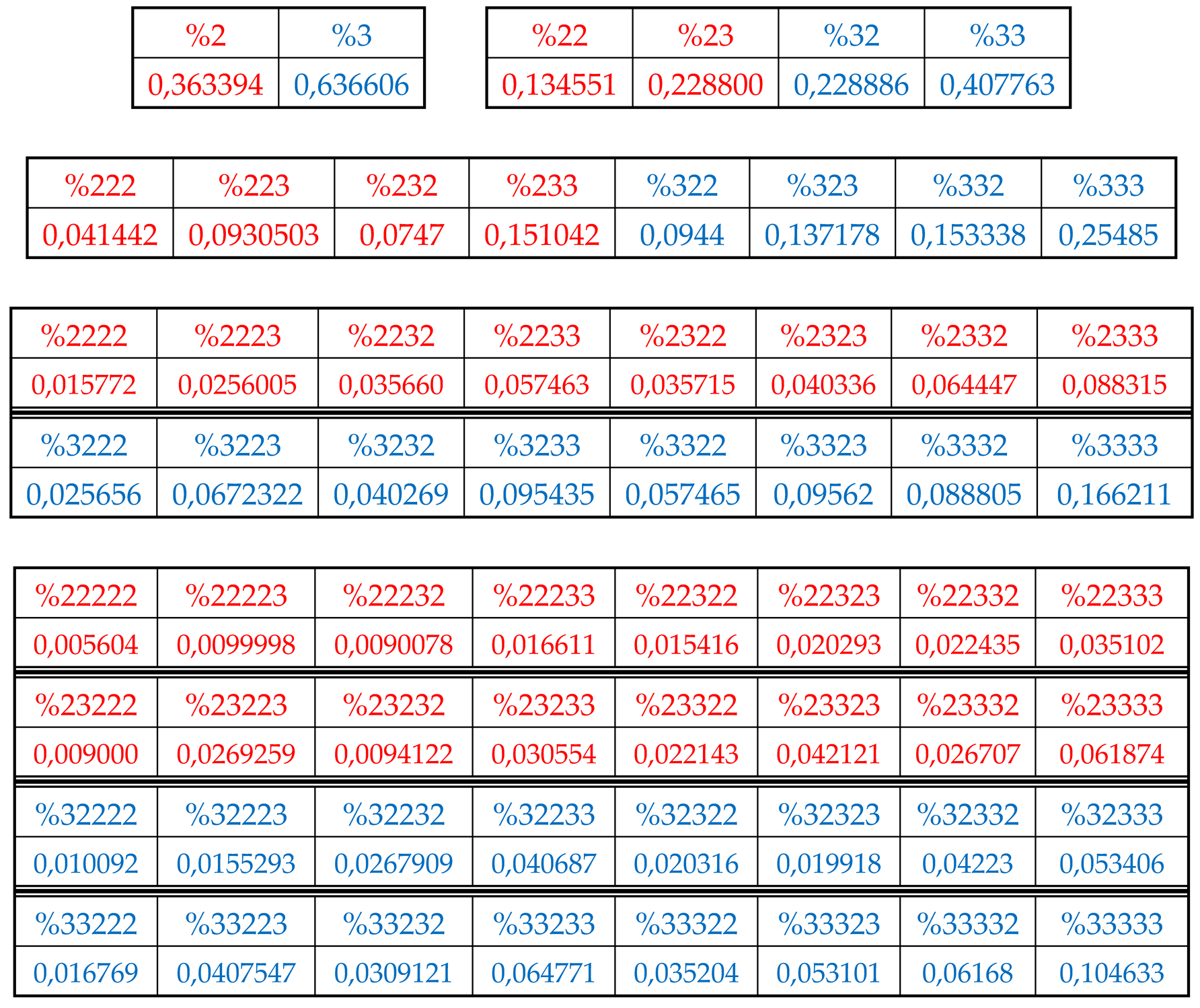Table 3 shows corresponding percent values of H-n-plets in genomic DNA of this bacteria.

Table 3. Phenomenological percent values of each of the H-n-plets in corresponding H-n-plets representations of the DNA of the bacteria Bradyrhizobium japonicum strain E109 (https://www.ncbi.nlm.nih.gov/nuccore/CP010313.1?report=genbank). Even H-n-plets starting with an even number 2 are in red, and odd H-n-plets starting with an odd number 3 are in blue.

Using these data of Table 3, any reader can check that dichotomic rules of H-n-plets percentages, described above for the human chromosomal DNA and for the chromosomal DNA of the plant Arabidopsis thaliana, hold as well in the genomic DNA of the bacteria Bradyrhizobium japonicum strain E109. For example, Figure 33 and Figure 34 show fractal trees in the case of the suffix dichotomy and the prefix dichotomy of percent values of H-n-plets for the genomic DNA of this bacteria.

Figure 33. At the top: the beginning of the fractal dichotomic percentage trees of H-n-plets, which is based on the algorithm of the suffix dichotomy. The case of genomic DNA of the bacteria Bradyrhizobium japonicum strain E109 is presented. Rounded numeric data of percentages are taken from Table 3. The left and the right columns present a practical invariance of sums of percentages of even and odd H-n-plets at all the levels (compare with Figure 25 and Figure 32). At the bottom: the diagram of comparative values of percentage sums at different levels of these fractal trees.

Figure 34. The beginning of the fractal dichotomic percentage trees of H-n-plets, which is based on the algorithm of the prefix dichotomy. The case of genomic DNA of the bacteria Bradyrhizobium japonicum strain E109 is presented. Rounded numeric data of percentages are taken from Table 3. The left and the right columns present a practical invariance of sums of percentages of even and odd H-n-plets at all the levels.

Again, each of the members of these parental fractal trees of probabilities (for example, %23) serves as a top of its own dichotomous fractal tree by analogy with the example in Figure 28).

8. Universal algorithms for dichotomies of probabilities in purine-pyrimidine sequences of genomic DNAs

In addition to the above-described phenomena of percent dichotomy of n-plets of hydrogen bonds in genomic DNAs, there are similar phenomena of percent dichotomies in other binary representations of genomic DNAs, which are described below.

As it was noted in the beginning of the article, the four nucleotides A, T, C, G of DNA are interrelated by their symmetrical peculiarities into the united molecular ensemble having the three pairs of binary-oppositional traits or indicators: strong-and-weak hydrogen bonds, purines-and-pyrimidines, and keto-and-amino.

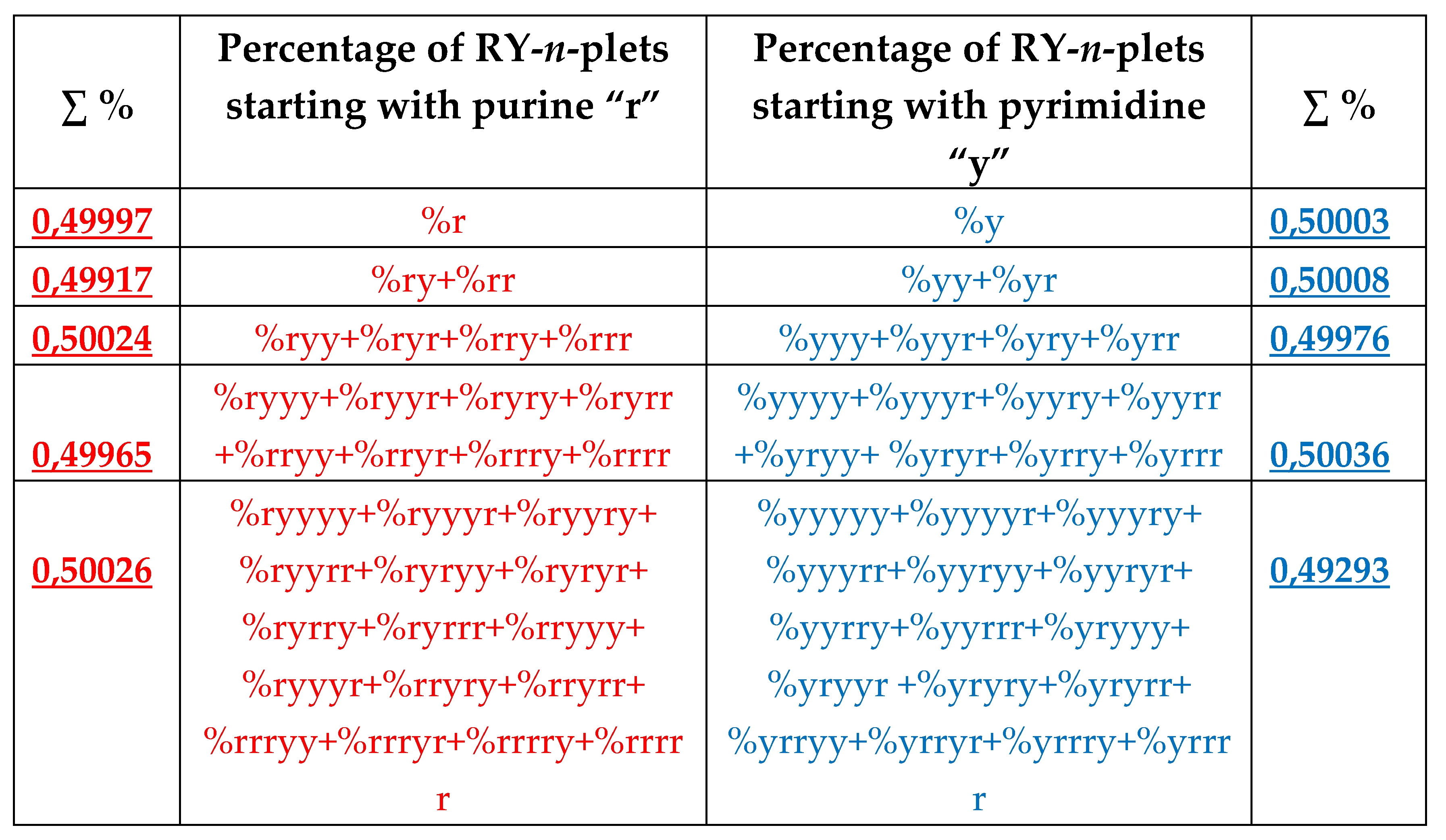
Above we described the universal rules of dichotomies for percent values of n-plets only for the case of the binary representation of genomic DNAs on the basis of binary-oppositional indicators of weak and strong hydrogen bonds 2 and 3. Now let us study the case of another binary representation of single-stranded genomic DNAs on the basis of binary-oppositional indicators of purines and pyrimidines. In genetics, purines (A and G), having 2 rings in their molecules, are traditionally denoted by the symbol “r”, and pyrimidines (T and C), having 1 ring in their molecules, by the symbol “y”. Correspondingly, we will study single-stranded genomic DNAs as binary sequences of purines and pyrimidines, that is, the symbolic RY-sequences like as ryyryrrryy… with the described HBS-method analyzing in this case percent values of n-plets of purine and pyrimidine (that is, RY-n-plets) in appropriate representations of the considered genomic DNA.

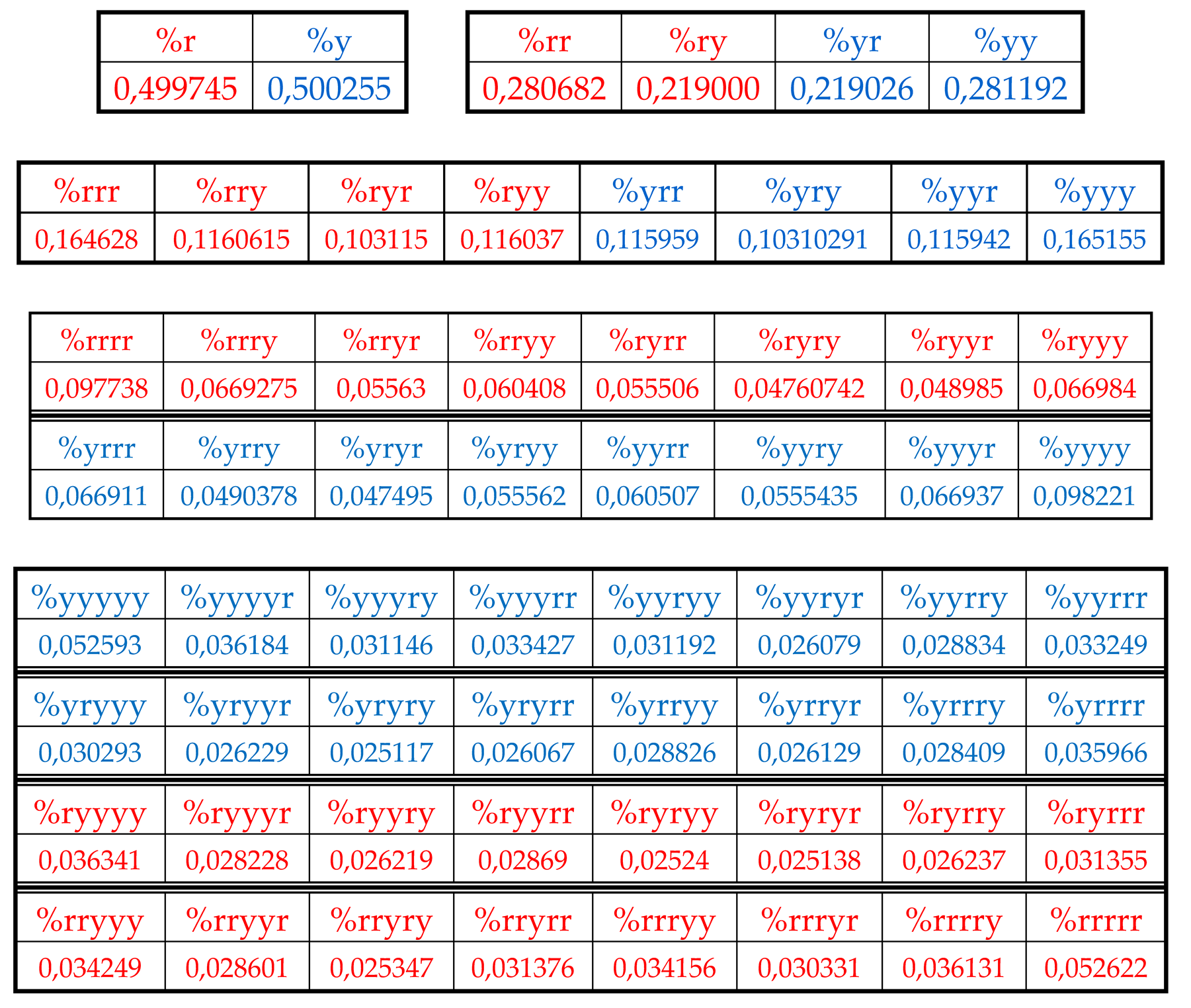
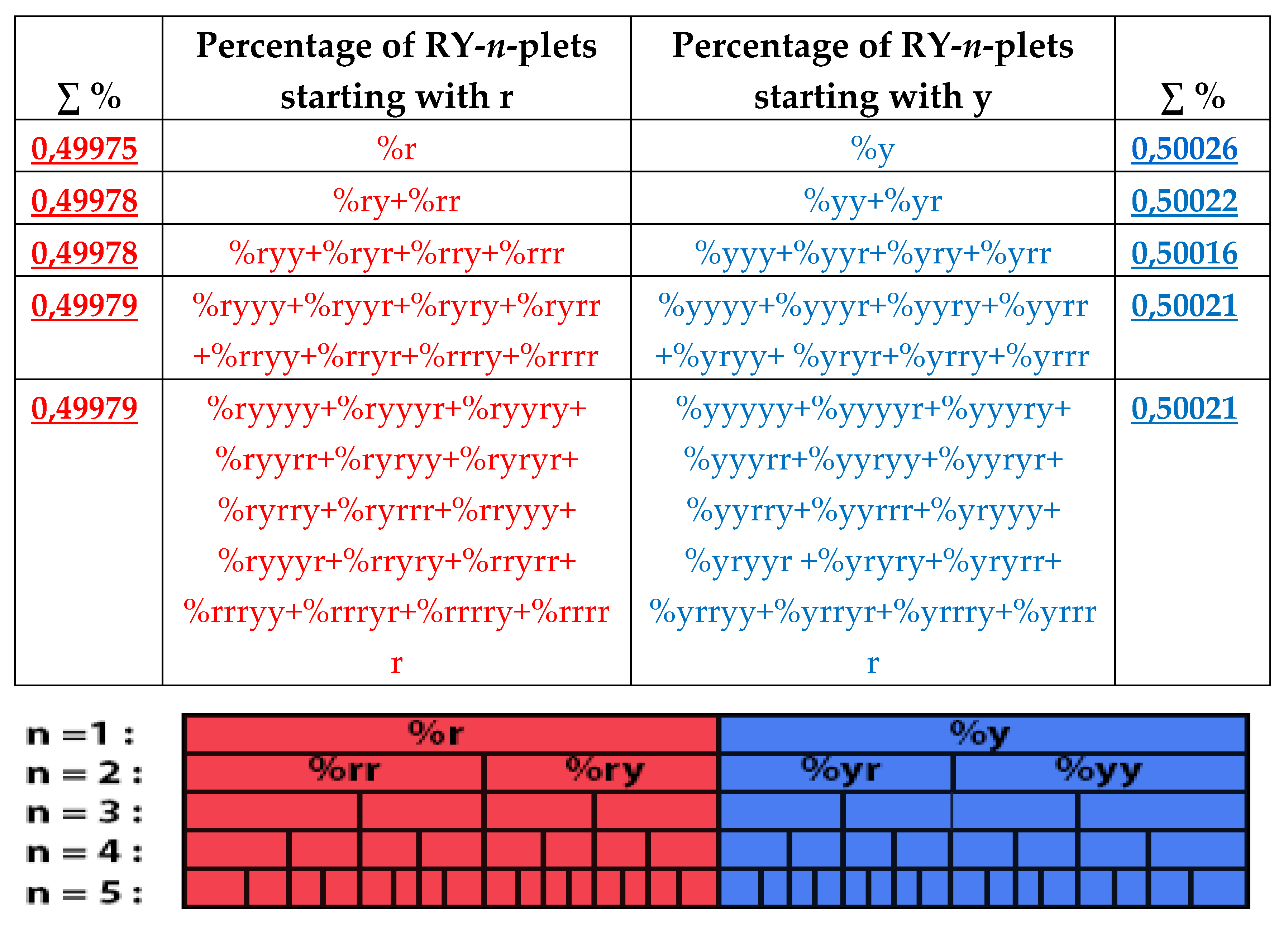
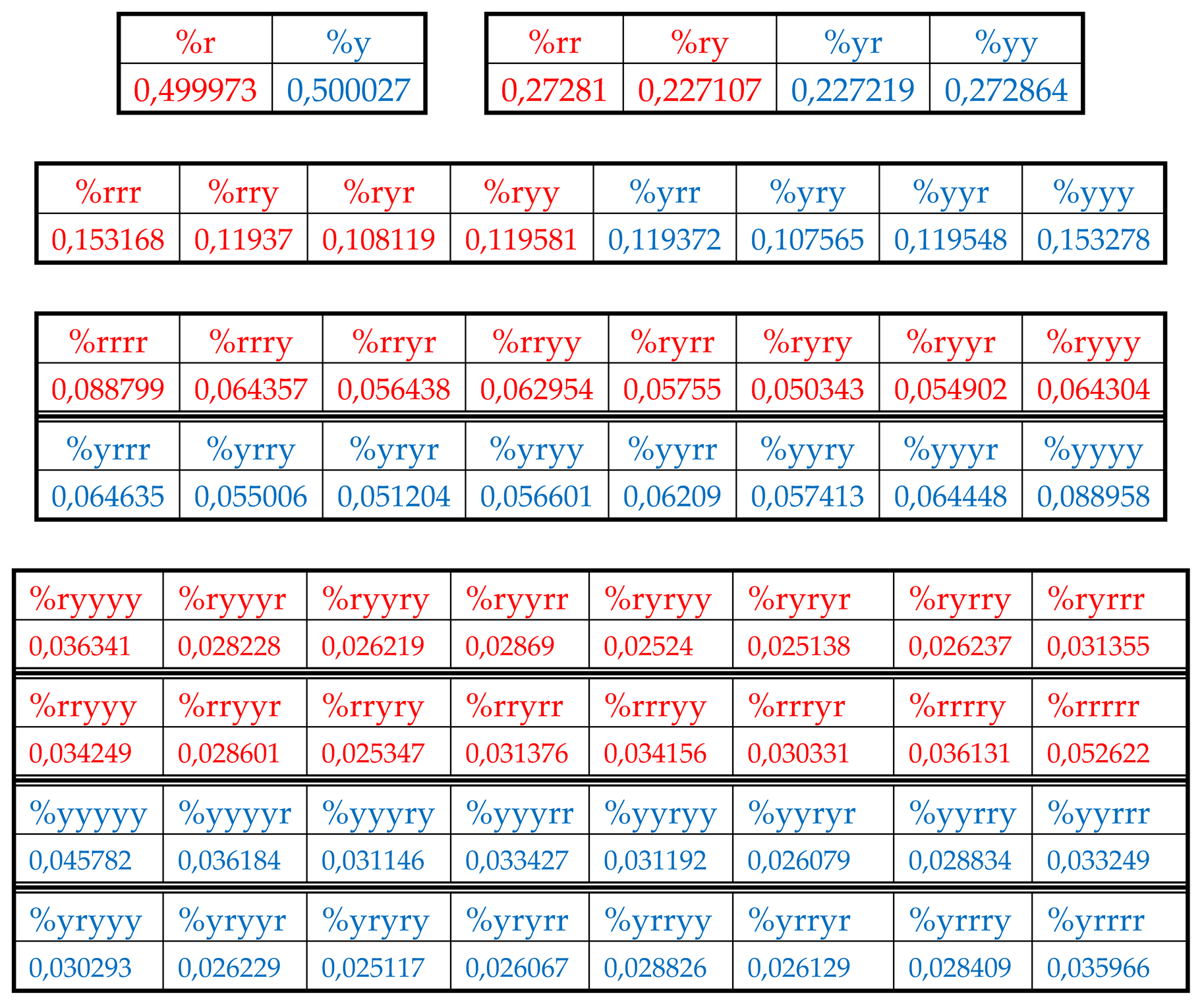
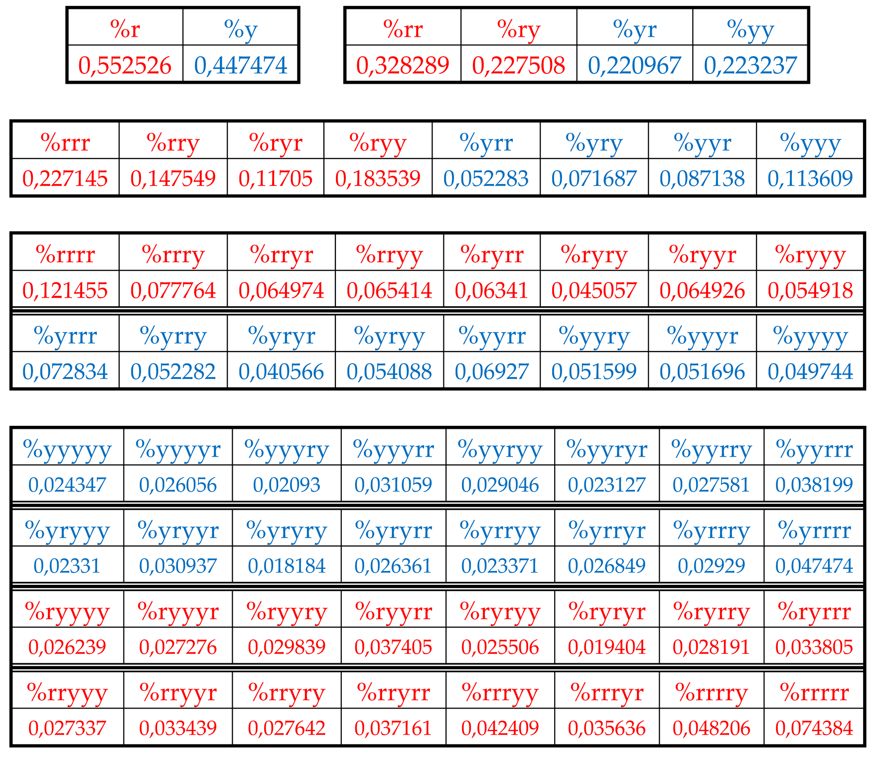
Let us return to single-stranded DNA of human chromosome № 1 to study percent values of RY-n-plets in its RY-sequence with the HBS-method. Table 4 shows percent values of RY-n-plets in this chromosomal DNA.

Analysis of the phenomenological data in Table 4 reveals that purine-pyrimidine sequences of the genomic DNA obey the same dichotomy rules for the percentage values of purine-pyrimidine n-plets, which are similar to dichotomic rules described above for the case of hydrogen bond n-plets. Let us demonstrate this with a few concrete examples.

8.1. Suffix dichotomies of percentages of n-plets in the purine-pyrimidine sequence of DNA of human chromosome № 1

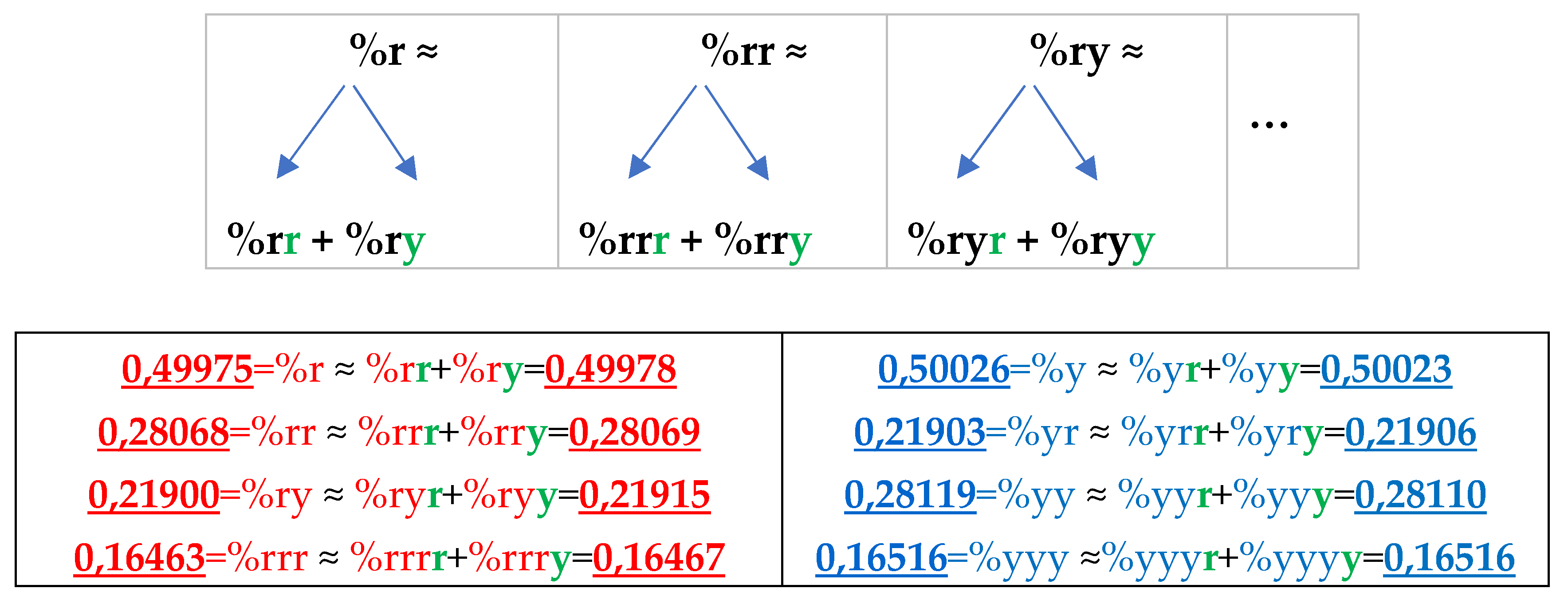
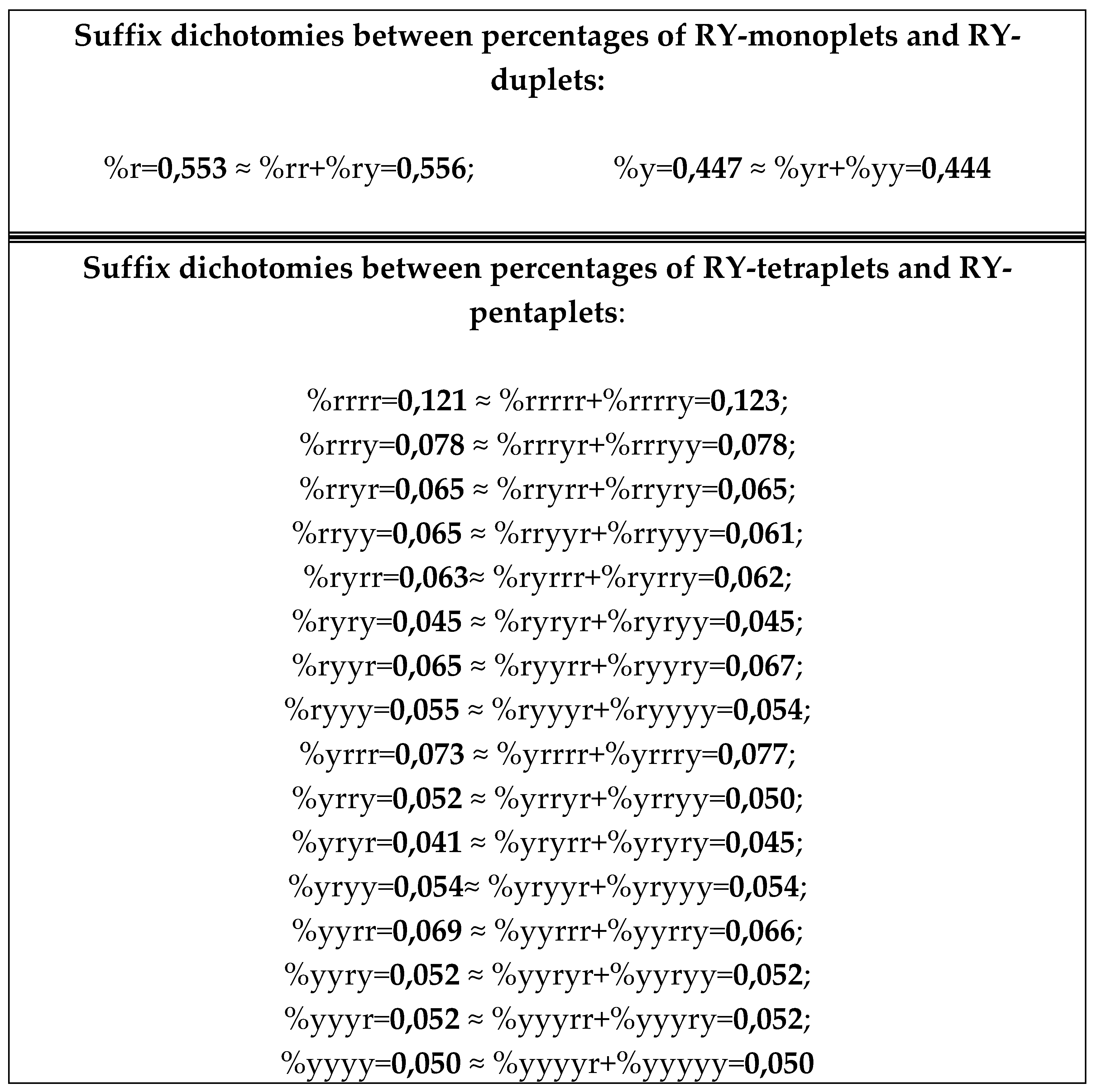
Analysis of the phenomenological data in Table 4 reveals the following: the percentage of any RY-n-plet is practically equal to the sum of percentages of those two RY-(n+1)-plets, which are generated from this RY-n-plet by addition the suffixes r and y to it as Figure 35 illustrates with separate examples.

Figure 35 represents only a few examples of high-precision equality of the percentages. Using numeric data from Table 4, any reader can check himself that such equalities of percentage dichotomies also hold with similar high precisions for all other possible variants of the noted percentages dichotomy. The author has systematically checked these percentage dichotomic equalities in many genomic DNAs, listed below, only for n = 1, 2, 3, 4, 5. He also selectively checked the fulfillment of such equalities for higher values of n getting positive results in every case, but he did not check at what values of n these dichotomic percentage equalities cease to hold.

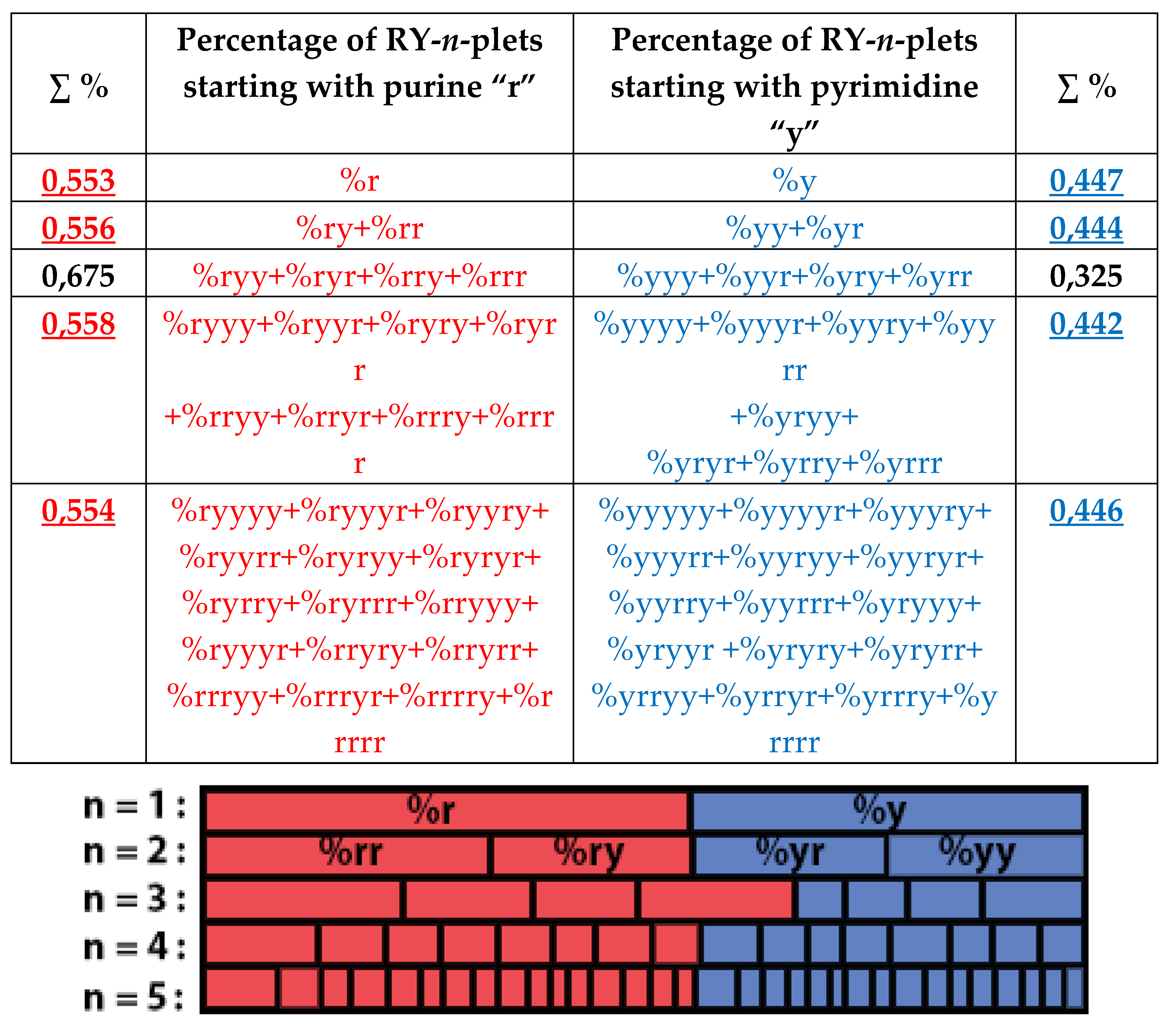
The rule of the suffix dichotomy of RY-n-plets percentages leads to fractal dichotomous trees of RY-n-plets percentages, which is shown in Figure 37 for the case of DNA of human chromosome № 1. RY-n-plets starting with a purine r (having even number 2 of molecular rings) are conditionally called even RY-n-plets (their percentages are marked by pink in Figure 36 and further), and RY-n-plets starting with pyrimidine y (having 1 ring) are called odd RY-n-plets (their percentages are marked by blue in Figure 36 and further). Each of the levels of these fractal trees with percentage values of even and odd RY-n-plets corresponds to a certain magnitude of n.

Levels of the trees of percentages in Figure 36 contain different quantity of percentage summands, but their sums remain the same with high precision at all the levels: in the tree of even RY-n-plets, the sums of percentages of even RY-n-plets are equal to 0.4998, and in the tree of odd RY-n-plets, the sums of percentages of odd RY-n-plets are equal to 0,5002. These summary values on the different levels are equal to the percentages of RY-monoplets: %r and %y. In the whole, in the considered case of the purine-pyrimidine sequences of RY-n-plets of the chromosomal DNA, we have a situation, which is very similar to the above-presented situation with n-plets of hydrogen bonds including the case of the prefix dichotomies (Figure 24, Figure 25, Figure 26, Figure 27, Figure 28, Figure 29, Figure 30 and Figure 31) as any reader can check himself. In particular, again, each of the members of these parental fractal trees of probabilities serves as a top of its own dichotomous fractal tree by analogy with the example in Figure 28. 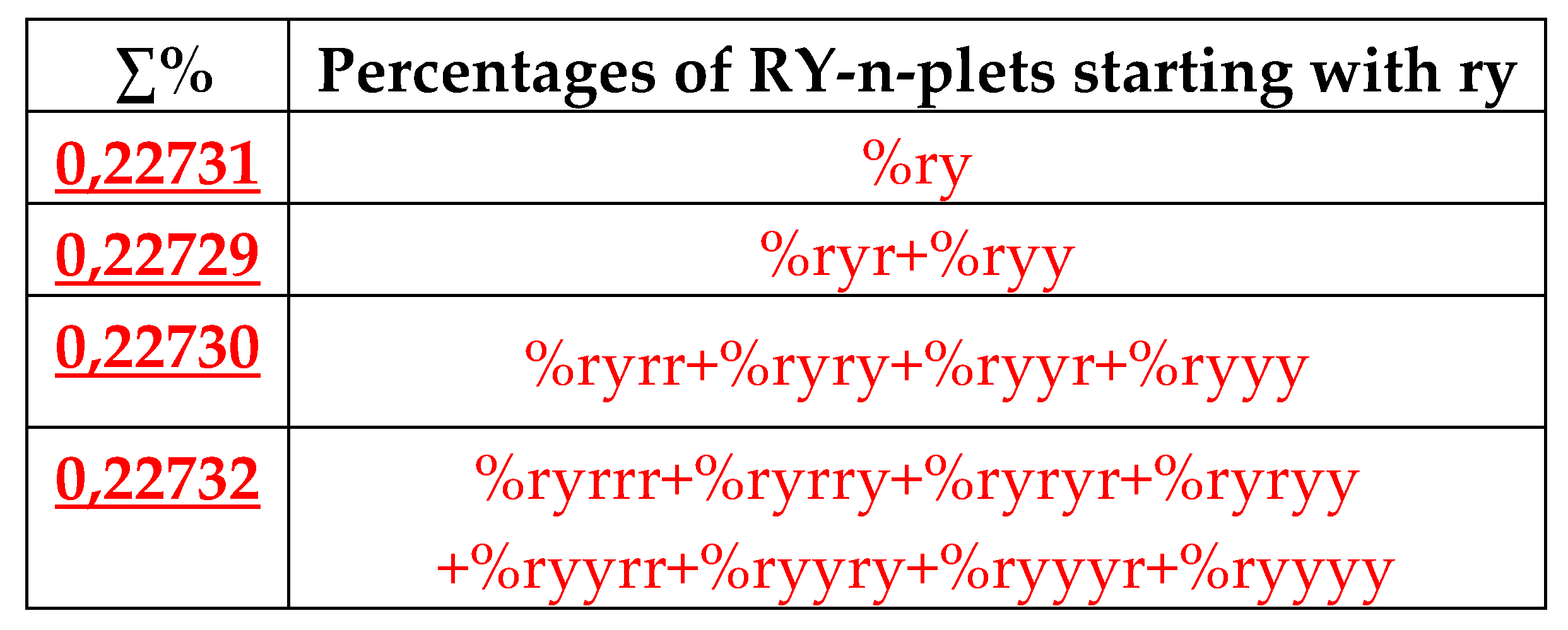Figure 37 illustrates this for the case of %ry, which serves as a top of its own dichotomous fractal tree.

But in the case of percentages of RY-n-plets in genomic DNAs, the additional interesting rule exist, which is presented in the next section.

8.2. Percent palindromes and the rule of equality of percent values of complementary purine-pyrimidine n-plets in genomic DNAs

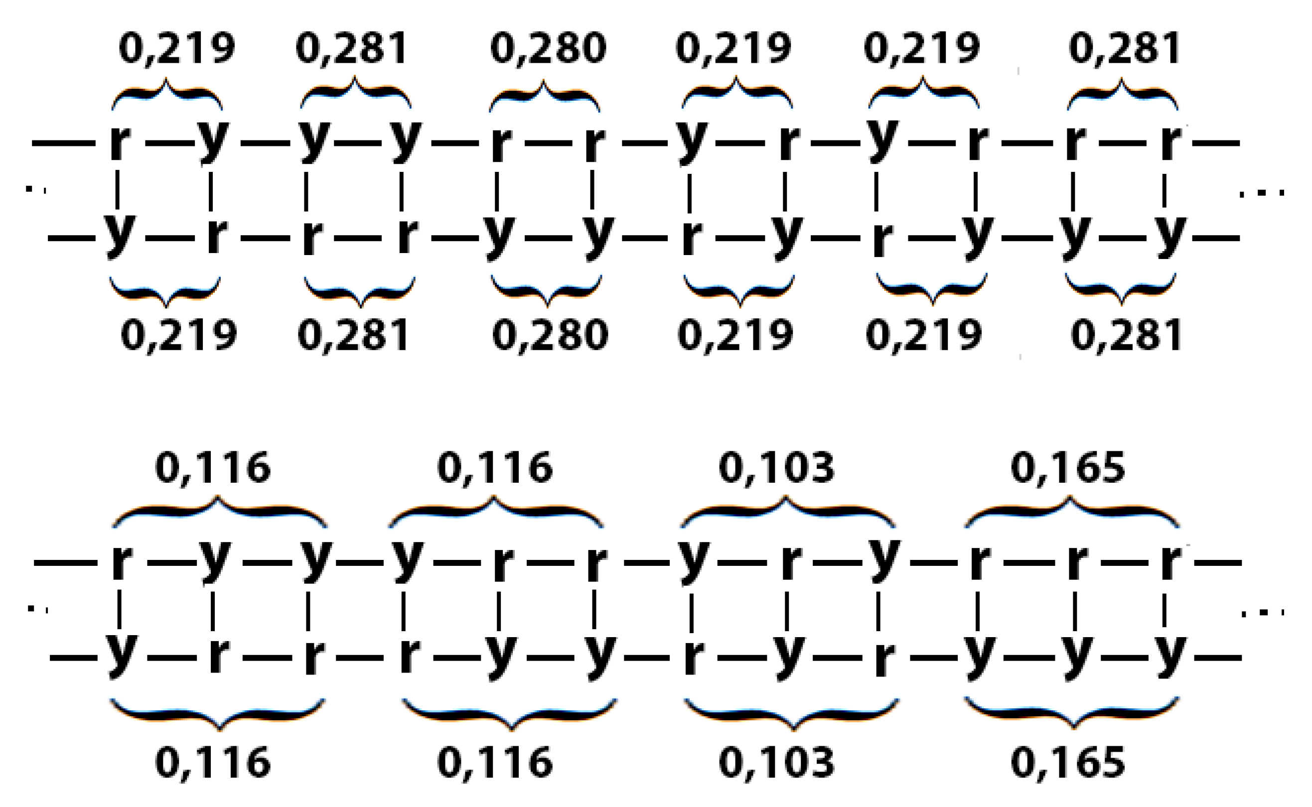
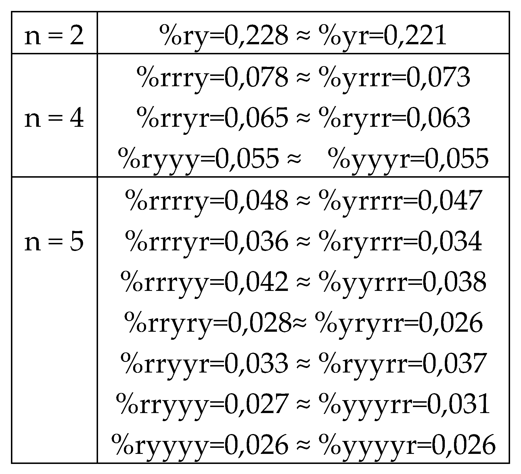
One can see in Figure 37 the mirror symmetry between left and right halves of the diagram regarding the width of the intervals at each of the levels of the fractal dichotomic percentage trees of n-plets of purines (r) and pyrimidines (y). This mirror symmetry is the consequence of the phenomenological rule of practical equality between percent values of those two RY-n-plets whose expressions are transformed each into another with the operation of complementary inversion r↔y (purine ↔ pyrimidine). For example, %rrr=0,165 ≈ %yyy=0,165, %yrrr=0,06691 ≈ %ryyy=0,06698, and so on (see Table 4).

The rule can be called the rule of the complementarity of percent values of complementary RY-n-plets in binary RY-n-sequences of genomic DNAs. It has some relations with complementary structure of double-stranded DNAs. Figure 38 illustrates this with examples of a double-stranded DNA having arbitrary sequences of purines and pyrimidines, which are presented here as sequences of duplets and triplets.

If purine r and pyrimidine y are denoted by binary symbols 0 and 1 correspondingly, then alphabetic sets of numberings of RY-n-plets in Table 4 contain their binary numberings in ordered form, specified as a dyadic group of binary numbers. With this ordering, the set of percentages for each fixed n turns out to be a palindrome of probabilities. For example, according to Table 4, the dyadic group of 3-bit binary numberings of RY-triplets 000, 001, 010, 011, 100, 101, 110, 111 is connected with the following palindrome of percent values: 0.165 - 0.116 - 0.103 - 0.116 - 0.116 - 0.103 - 0.116 - 0.165. In biology, as one of the mysteries of the genetic system, the problem of the wide distribution of palindromes in DNA nucleotide sequences has long been known. In genetics, the topic of palindromes has been the subject of tens of thousands of publications, since the DNA texts of different genomes contain an abundance of palindromes. In the human genome, about a third of DNA texts are represented by them [Gusfield, 1997]. In evolutionary biology, the abundance of such palindromes in genomes is considered as evidence that DNA texts are not random, that they are not reducible to a set of random mutations. What is the relationship between the above-described probability palindromes and the known molecular palindromes of nucleotide sequences? This is an open question at this stage of research.

8.3. Suffix dichotomies of percentages of n-plets in the purine-pyrimidine sequence of DNA of the chromosome № 1 of the plant Arabidopsis thaliana

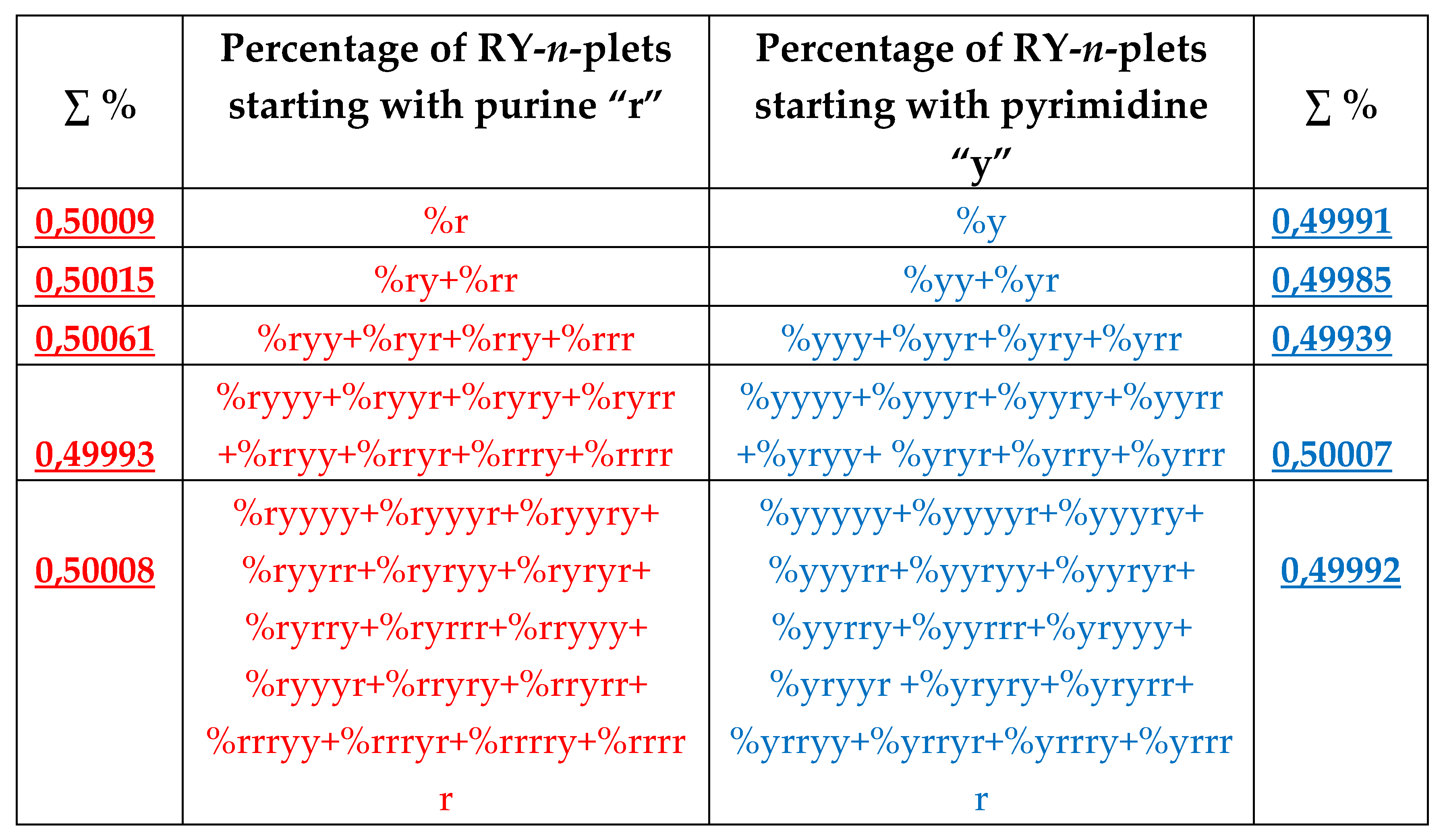
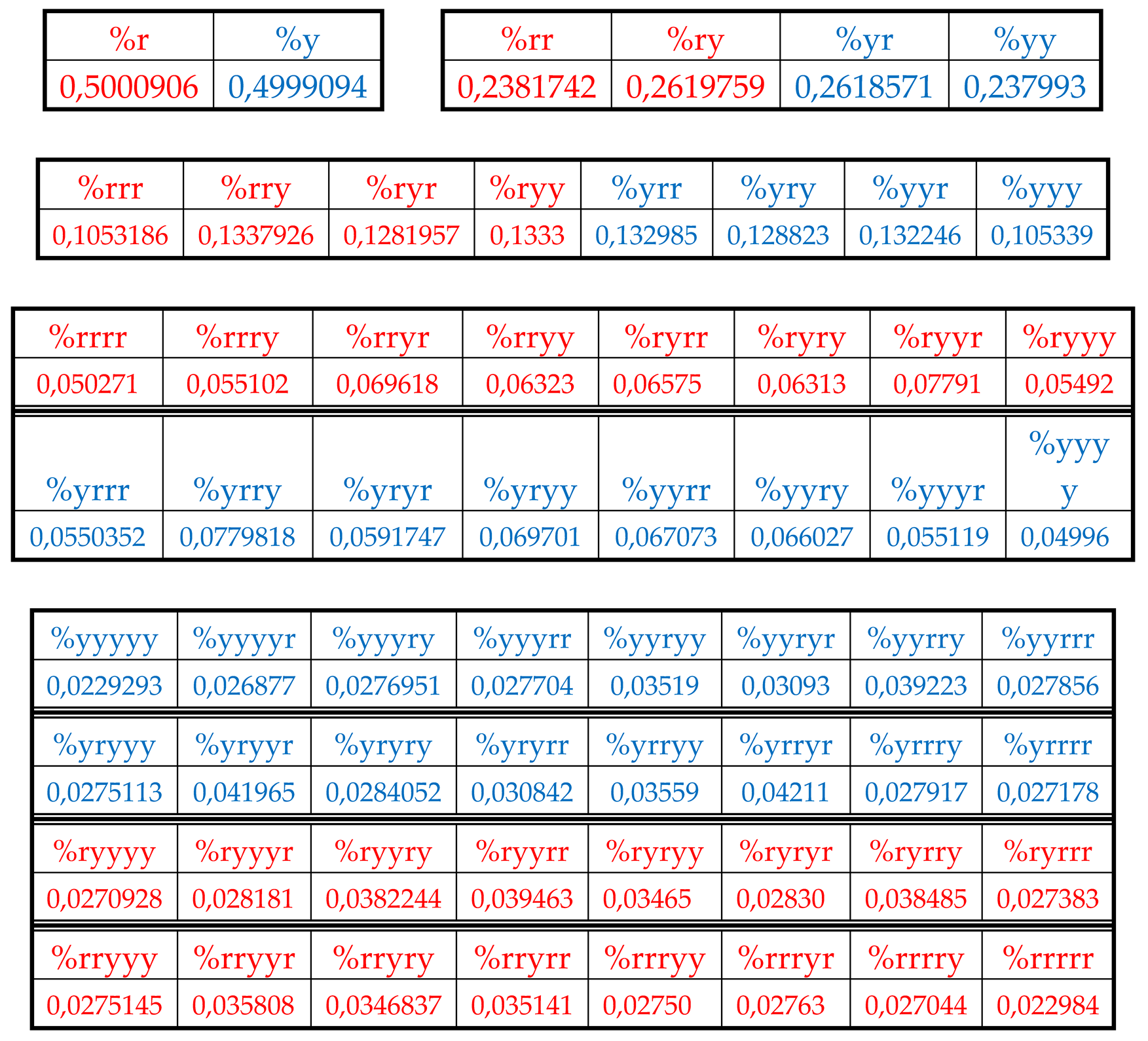
Table 5 shows percent values of RY-n-plets in the RY-sequence of the DNA chromosome № 1 of the plant Arabidopsis thaliana.

Analysis of the phenomenological data in Table 5 reveals the following: the percentage of any RY-n-plet is practically equal to the sum of percentages of those two RY-(n+1)-plets, which are generated from this RY-n-plet by addition to it the suffixes r and y as Figure 39 illustrates with separate examples.

Comparison of Figure 37 and Figure 40 shows the similarity of stochastic organization of binary purine-pyrimidine sequences of the considered chromosomal DNAs of human and the plant Arabidopsis thaliana. In both cases, fractal dichotomous trees arise when these DNAs are analyzed by the NIH method. The above-formulated rule of the complementarity of percent values of complementary RY-n-plets holds in this chromosomal DNA as well. Again, each of the members of these parental fractal trees of probabilities serves as a top of its own dichotomous fractal tree by analogy with the example in Figure 28.

8.4. Suffix dichotomies of percentages of n-plets in the purine-pyrimidine sequence of DNA of bacteria Bradyrhizobium japonicum

Table 6 shows percent values of RY-n-plets in the RY-sequence of the genomic DNA of bacteria Bradyrhizobium japonicum strain E109 (complete genome, 9224208 bp) were taken from https://www.ncbi.nlm.nih.gov/nuccore/CP010313.1?report=genbank.

Analysis of the phenomenological data in Table 6 reveals again the following: the percentage of any RY-n-plet is practically equal to the sum of percentages of those two RY-(n+1)-plets, which are generated from this RY-n-plet by addition to it the suffixes r and y. Figure 41 shows corresponding fractal dichotomic percentage trees in the case of this bacterial genomic DNA.

Comparison of Figure 37, Figure 40 and Figure 41 shows the similarity of stochastic organization of binary purine-pyrimidine sequences of the considered genomic DNAs. Fractal dichotomous trees arise systematically when these DNAs are analyzed by the NIH method. The above-formulated rule of the complementarity of percent values of complementary RY-n-plets holds in this bacterial genomic DNA as well. Again, each of the members of these parental fractal trees of probabilities serves as a top of its own dichotomous fractal tree by analogy with the example in Figure 28.

9. Universal algorithms for dichotomies of probabilities in keto-amino sequences of genomic DNAs

Now let us turn to the third binary sub-alphabet of DNA based on the binary opposition “keto-vs-amino”. A pair of nucleotides G and T contains a keto group and are designated on this basis in genetics by the generally accepted symbol K, and another pair of nucleotides A and C contains an amino group and are designated on this basis by the symbol M. The keto group is characterized by the presence of a molecular bond of carbon and oxygen C=O , and the amino group - by the presence of a molecular bond of carbon and oxygen with hydrogen C-OH. The serial number of oxygens in the periodic table of Mendeleev is equal to the even number of protons 8, and the number of protons in the amino group OH is equal to the odd number 9. Therefore, if desired, we can say that the binary sequences of keto and amino groups in single-stranded DNA are conditionally binary sequences of even and odd numbers 8 and 9. Below we are presenting a few results of study of sequences of keto- and amino-groups on the DNAs of human chromosome № 1, chromosome № 1 of the plant Arabidopsis thaliana and the bacteria Bradyrhizobium japonicum (just these DNAs have been used above as examples for the demonstration of dichotomic fractal trees in cases H-n-plets and RY-n-plets).

9.1. Suffix dichotomies of percentages of n-plets in the keto-amino sequence of DNA of human chromosome № 1

Table 7 shows percent values of n-plets in the binary sequence of keto- and amino-groups (or keto- and amino-indicators) in DNA of human chromosome № 1 with the HBS-method. Such binary sequences revealed with HBS-method are denoted as KM-sequences.

Analysis of the phenomenological data in Table 7 confirms the principle of percentage dichotomies of KM-n-plets in this human chromosomal DNA. Figure 42 shows corresponding dichotomic fractal trees, which are very similar to the dichotomic fractal trees in the case of n-plets of purines and pyrimidines in Figure 37.

The left and right halves of the percent diagram in Figure 42 are mirror-symmetrical each to another from the point of view of width of their intervals. It is connected with the fulfillment of the rule of the practical equality of percent values in complementary KM-n-plets in binary KM-n-sequences of the genomic DNA by analogy with the above-described case of n-plets of purines and pyrimidines. According the author’s results of analysis of the named set of genomic DNAs, this rule is a general for all tested genomes and now is a candidacy to be an universal genomic rule (like a similar rule for RY-n-plets considered above).

Again, each of the members of these parental fractal trees of probabilities (Figure 42) serves as a top of its own dichotomous fractal tree by analogy with the example in Figure 28.

9.2. Suffix dichotomies of percentages of n-plets in the keto-amino sequence of DNA of chromosome № 1 of the plant Arabidopsis thaliana

Table 8 shows percent values of n-plets in the binary KM-sequence of keto- and amino-groups in DNA of chromosome № 1 of the plant.

Analysis of the phenomenological data in Table 8 reveals the similar situation with percent dichotomies in this chromosomal DNA of the plant: the percentage of any KM-n-plet is practically equal to the sum of percentages of those two KM-(n+1)-plets, which are generated from this KM-n-plet by addition to it the suffixes K and M. Figure 43 shows corresponding dichotomic fractal trees of percentage of KM-plets. The rule of practical equality of percent values of complementary KM-n-plets in binary KM-n-sequences holds for this plant chromosomal DNA as well.

The rule of the practical equality of percent values in complementary KM-n-plets in binary KM-n-sequences of this chromosomal DNA holds as well. Again, each of the members of these parental fractal trees of probabilities serves as a top of its own dichotomous fractal tree by analogy with the example in Figure 28.

9.3. Suffix dichotomies of percentages of n-plets in the keto-amino sequence of the genomic DNA of the bacteria Bradyrhizobium japonicum

Table 9 shows percent values of n-plets in the binary KM-sequence of keto- and amino-groups in the genomic DNA of the bacteria Bradyrhizobium japonicum

Analysis of the phenomenological data in Table 9 reveals the similar situation with percent dichotomies in this bacterial genomic DNA: the percentage of any KM-n-plet is practically equal to the sum of percentages of those two KM-(n+1)-plets, which are generated from this KM-n-plet by addition to it the suffixes K and M. Figure 44 shows corresponding dichotomic fractal trees of percentage of KM-plets. The rule of practical equality of percent values of complementary KM-n-plets in binary KM-n-sequences holds for this bacterial genomic DNA as well.

Again, each of the members of these parental fractal trees of probabilities serves as a top of its own dichotomous fractal tree by analogy with the example in Figure 28.

10. Parallelism between dichotomies in inherited biological bodies and universal dichotomies of probabilities in stochastic organization of genomic DNAs

The described results give pieces of evidence about existence of universal rules of dichotomies of probabilities (percentages) in stochastic organization of genomic DNAs of higher and lower organisms. These rules lead to existence of a wide set of dichotomic fractal trees of probabilities for cases of different modalities (for the binary oppositions of “strong and weak hydrogen bonds”, “purine and pyrimidine”, “keto and amino”). These basic or “parental” fractal trees of probabilities include their “daughter” fractal dichotomic trees of probabilities since each of their percentage members serves as a top of its own dichotomic fractal tree of probabilities as it is shown above.

Genomic informatics turns out to be associated with networks of many interconnected fractal trees of dichotomies of probabilities in genomic DNAs. Accordingly, for example, the genomic percentage of each triplet of nucleotides turns out to be simultaneously a member of many described dichotomy trees of probabilities existing in any genomic DNA.

The described universal rules of dichotomies of probabilities in genomic DNAs have been discovered on the basis of the author’s method of hierarchical binary stochastics (HBS-method), which represents any genomic DNA as a multi-level hierarchical set of stochastic sequences of n-plets, where each of the text-like sequences uses the corresponding n-plets alphabet containing 2ⁿ-members. Such representation resembles traditional Russian dolls “Matryoshka” based on the hierarchical nesting of objects of different sizes into each other (Figure 45). In the light of this analogy, the author’s HBS-method can also be simplistically called “the stochastic matryoshka method”.

The noted universal rules of dichotomies of probabilities of different modalities in genomic DNAs testify to the existence of non-trivial algebraic invariants of a global genomic nature, which remain unchanged over billions of years of biological evolution, during which millions of species of organisms die off and new ones arise (although locally genomic sequences are changed by mutations, the pressure of natural selection, etc.).

Dichotomies in genetically inherited biological bodies and their transformations are well known. Their examples give, for example, the functioning of double-stranded DNA; mitosis of somatic cells; branching in plants; the bronchial tree of the human lungs with its 23 levels of dichotomies (there are approximately 2²³ = 8,388,608 alveoli at the end of the bronchial tree branches [Medvedev, 2020]; dichotomous branching of neuronal axons and dendrites (there are no branching for three, four, five, and so on [Tsang, 2016, p.235]). Presented in Figure 25 and Figure 31, asymmetric pairs from the left and right dichotomous trees, which are connected with even and odd numbers 2 and 3, are associated with two genetically inherited asymmetric cerebral hemispheres endowed with different functions. The Yin-Yang theme (left and right, even and odd, feminine and masculine) that is cross-cutting for biology and culture is systematized in a well-known book published in different languages with the characteristic title “Even and Odd. Asymmetry of the brain and sign systems” [Ivanov, 1978]. This feature of the dichotomy of percentages of hydrogen bonds 2 and in genomic DNA allows us to recall some historical facts that, for example, in ancient China, the numbers 2 and 3 were considered the numbers of Yin and Yang (or female and male numbers) and also as numbers of the Earth and the Sky; these numbers served as the basis of ancient Chinese arithmetic.

But in genomic DNAs, in contrast to bodily biostructures, we encounter a fundamentally different type of dichotomy: the dichotomies of stochastic (probabilistic) characteristics in DNA information sequences. The vast dichotomous fractal networks of genomic DNA probabilities are the soil from which living bodies and genetic intelligence grow. The material structures of living bodies do not arise from scratch, but have structural prototypes in a regular system of biological probabilities in a variety of genetic languages with their families of 2ⁿ-parameter alphabets. Here it should be recalled that genetics as a science began with the discovery by Mendel of the rules of stochastic (probabilistic) inheritance of traits in experiments on crossing organisms. Many processes in living bodies are stochastic. Even genetically identical cells in the same tissue have different levels of protein expression, different sizes and structure due to the stochastic nature of the energy interaction of individual molecules in cells. The stochastic nature of the inheritance of traits in the “small scale” is fundamentally different from the deterministic inheritance of traits in the “large scale”. For example, the fingerprints of the fingertips are different for all people, despite the fact that the fingers as a whole are determined with their shapes and structures (3 phalanges, etc.). Thus, biological phenomena are associated with the dualism “stochastics-determinism”.

According to Mendel’s law of independent inheritance of traits, information from the level of DNA molecules are reflected in the macrostructure of living bodies through many independent channels despite strong noise. Thus, the colors of hair, eyes and skin are inherited independently of each other. Accordingly, each organism is a multi-channel noise-immune coding machine. The author believes that the future of biology is connected with the study of a deep and regular structured system of probabilities in the world of stochastic energies of interaction in material media.

One of the interesting areas of future research is the analysis of the relationship between the traditionally studied dichotomous fractals in the configurations of biological bodies and the above-described dichotomous percentage fractals in the stochastic (probabilistic) organization of genomic DNA. Fractals (or fractal-like structures) in the configurations of biological bodies is studied long ago, in particular, in connection with cancer, and is presented, for example, in the works [Pellionisz, 1989; Pellionisz et al., 2013; Werner, 2010]. The book [Tsang, 2016], which has the characteristic title “Fractal Brain Theory”, contains rich material on biological fractals, including literary references to thematic publications of various authors.

Revealing the universal rules of stochastic dichotomies in genomes allows us to rethink the phenomena of dichotomies in the inherited structures of biological bodies. Life on Earth has existed for at least 3.5 billion years, and all this time the genetics of organisms and the genetically inherited organisms themselves are built on a dichotomy.

For example, over the course of billions of years of life on Earth, it is typical for bacteria and prokaryotes in general to reproduce by dichotomous division of the body into two halves. What are the structural foundations for this “eternal” dichotomous phenomenon of bacterial reproduction, which is accompanied by the most complex processes of dichotomous separation of all dichotomously organized genetic information, together with the accompanying multi-species protein and nucleic assemblies inside a bacterial cell?

The author suggests the following possible answer to such questions. There is a world of families of probabilities, hidden from direct perception and structured on the basis of binary oppositions (like Yin-Yang), reminiscent, in particular, of binary oppositions in physics: positive and negative electric charges, the north and south poles of magnets, the forces of attraction and repulsion, etc. It is in the image and likeness of the binary organized families of probabilities of this world that genetically inherited biological bodies are built. Figuratively speaking, our bodies are clothes put on these binary structured families of probabilities, which act as prototypes of biological structures and are endowed with their own forms of energy. To a certain extent, this is similar to the situation with the invisible man from the novel “The invisible man” by H.G. Wells, whose invisible figure becomes definable only when he is wearing clothes. It is also reminiscent of the ancient concepts of the manifested and the non-manifested worlds, and Plato’s famous allegory of the world of ideas and the shadows on the cave wall, by which people living in a cave can judge the true hidden world of ideas. By studying the universal rules of genomic DNAs, we indirectly research the rules of this hidden world of binary families of probabilities, which is the progenitor of biological structures with their amazing properties.

The idea of the regular world of stochastic energy processes as the basis of inherited biological structures is important, among other things, for understanding genetic intelligence. By genetic intelligence, we mean that part of the intellectual potency of living organisms that allows, on the basis of genetic information in DNA and RNA molecules, to build, for example, from one fertilized cell an organism with trillions of cells in such a way that parental characteristics are reproduced in it in a multichannel noise-resistant manner, despite strong noises and constantly changing conditions of food and external influences in the course of life. In this case, we are talking about a systematic growth - in the course of ontogenesis - of the number of body parameters and a corresponding increase in the dimension of its configuration space of states [Petoukhov, 2022c]. This approach echoes the following opinion about the activity of the brain by R. Kurzweil, a well-known artificial intelligence specialist: the brain is a probabilistic recursive fractal that seems extremely complex, but in fact it may turn out to be much simpler than it seems [Tsang, 2016, p. 50].

With the development of physics and the emergence of quantum mechanics, people drew attention to the fundamental importance of the world of probabilities for understanding and modeling the objects and processes of the environment that they see. The described algebra-genetic studies complement the theme of the importance of the world of probabilities. The presented studies are consonant with the works of V. Nalimov (https://en.wikipedia.org/wiki/Vasily_Nalimov), who considered it his goal to build a probabilistic model of the language, and then of consciousness in general [Nalimov, 2015].

According to the results available to the author, the HBS-method (or the stochastic matryoshka method) is useful for the knowledge and comparative analysis of not only long genomic DNAs, but also relatively short DNAs of genes, in which the dichotomies of percentages inside of sets of n-plets are violated. It allows you to characterize the DNAs of each genome and each gene, figuratively speaking, with its individual the “fingerprint” of the stochastic organization of its binary representations and, in this regard, assign the DNA and RNA of each genome and each gene an individual “polyplet stochastic passport”. Such a polyplet stochastic certification of genetic sequences seems to be useful for revealing the relations of structural relationship of various genetic sequences.

This HBS-method is also useful for the development of “binary-stochastic rhythmology” due to the fact that many physiological rhythms, upon closer examination, are associated with binary sequences and stochastic fluctuations in them due to the stochastics of energy interactions in molecular media. For example, sequences of cardiac pulsations are characterized by stochastic fluctuations of cardio-intervals in them. These fluctuations of cardio-intervals, which have a diagnostic value, can be investigated by the named method in order to identify stochastic regularities such as dichotomies of the probabilities of the corresponding n-plets in their binary representations. In general, the named author’s method of DNA sequence analysis leads to new useful approaches for the development of evolutionary biology and personal genetics, as well as various branches of physiotherapy, pharmacology, art therapy and medical engineering. In particular, it has been successfully applied by the author in the analysis of the stochastic organization of long phonetic sequences of the Russian language (that is, sequences of sounds of four types - short and long vowels, voiceless and voiced consonants) on the material of volumetric texts of novels by A.N. Tolstoy, F.M. Dostoevsky, A.S. Pushkin, the Russian text of the Bible, etc. [Petoukhov, 2020a]. On this path of understanding the biological significance of polyplet stochastic regularities, new algebraic formalisms are introduced into genetic and physiological analysis, including formalisms of matrix genetics, metric analysis, quantum informatics, algebraic geometry, resonance theory, and antenna array theory [Petoukhov, 2008, 2018, 2021c, 2022b].

11. Regarding analysis of DNAs of genes with the HBS-method

Sequences of genomic DNAs consist of genes and fragments (introns) that do not code for proteins. For example, it is currently believed that there are 4234 genes on the human chromosome № 1, which are associated with 890 genetic diseases, including Alzheimer’s disease, Parkinson’s disease, glaucoma, breast and prostate cancer, etc. The total length of the sequences of these genes is only a small part of this chromosomal DNA, the rest of it is occupied by introns.

Since, as shown above, the application of the HBS-method (or the method of stochastic matryoshkas) to the analysis of genomic DNA yields important results, it is logical to apply it to the analysis of the constituent parts of genomic DNA, that is, to the analysis of genes and introns. In this section, we provide only one illustrative example of the application of this perspective method to gene analysis for revealing hidden rules and symmetries in stochastic organization of genetic sequences. For brevity, this analysis is called HBS-analysis.

Let us first consider the human TTN gene, having 81940 bp and encoding the protein Titin, which is the largest protein in humans. Titin, also known as connectin, is important in the contraction of striated muscle tissues. The length of the DNA sequence of this longest gene is about 3000 times shorter than the length of the DNA sequence of the human chromosome № 1 analyzed above (Table 1). But surprisingly, the sets of percentages of n-plets in this highly truncated DNA obey practically the same (except for the case n=3) rules for the dichotomous interconnections of percentages of n-plets with different values n in the binary representations of the DNA.

11.1. The HBS-analysis of the sequence of hydrogen bonds in the gene TTN

We begin with HBS-analysis of the binary representation of DNA of the gene TTN in a form of its H-plets sequence of hydrogen bonds 2 and 3 (by analogy with Table 1). Table 10 shows percent values of n-plets of hydrogen bonds in this binary sequence.

First of all, analysis of the phenomenological data in Table 10 reveals the following suffix dichotomous interconnections between presented probabilities of H-n-plets in the case of the gene TTN. The percentage of any H-monoplet is practically equal to the sum of percentages of those H-duplets, which are generated from this H-monoplet by addition of the suffixes 2 and 3 to it, for example, %2 ≈ %22+%23. The percentage of any H-tetraplet is practically equal to the sum of those H-pentaplets, which are generated from it by addition of the suffixes 2 and 3 to it, for example, %2222 ≈ %22222+%2223. Figure 46 shows these percentage dichotomous interconnections in detail with rounded percent values.

But for the case n=3, that is, for the shown percentage set of H-triplets, its dichotomous interconnections with neighboring percentage sequences of H-duplets and H-tetraplets are significantly disturbed in the considered TTN gene. One can recall here that nucleotide triplets encode amino acids of proteins.

By analogy with the dichotomy trees of the percentages of H-n-plets in genomic DNAs shown in Figure 25, it is possible to construct a tree of percentages of n-plets of hydrogen bonds 2 and 3 for the DNA of the analyzed gene. Figure 47 shows that at n=3 there is a significant violation of the dichotomy interconnections rule with the percent values of n-plets of neighboring levels (n = 2 and n = 4).

The case of the prefix dichotomies gives analogical results regarding percentages of H-n-plets in the gene.

In genomic DNAs, the rule of percentage equalities in the set of genomic H-n-plets holds (see above section 7.1.1 about DNA of human chromosome № 1): those two H-n-plets, which are read as mirror (or reversed) copies of each another (such as 223 and 322), always have almost the same percent values in the genomic H-n-plets sequence. This rule holds as well for studied cases n = 2, 4, 5 in the analyzed gene TTN though the length of its sequence is about 3000 times shorter than the length of the DNA sequence of the human chromosome No. 1. Figure 48 shows numerical data confirming this.

But for the case of n = 3, that is for the percentage sequence of H-triplets in the gene, this rule of percentage equalities is disturbed since this sequence has expressed percentages inequalities: %223=0,106 ≠ %322=0,186 and %233=0,072 ≠ %332=0,155. The reasons for such very special status of H-triplets sequence in the gene should be studied in the future.

11.2. The HBS-analysis of the purine-pyrimidine sequence of the gene TTN

Let us turn now to analysis of the DNA purine-pyrimidine sequence of the gene TTN of the human longest protein Titin. Table 11 shows percent values of n-plets of purines (r) and pyrimidines (y) in single-stranded DNA of this gene.

Analysis of the phenomenological data in Table 11 reveals the following. The percentage of any RY-monoplet is practically equal to the sum of percentages of those RY-duplets, which are generated from this RY-monoplet by addition of the suffixes “r” and “y” to it, for example, %r ≈ %rr+%ry. The percentage of any RY-tetraplets is practically equal to the sum of those RY-pentaplets, which are generated from it with addition of the suffixes r and y to it, for example, %rrrr ≈ %rrrrr+%rrrry. Figure 49 shows these percentage dichotomous interconnections in detail with rounded percent values.

But for the case n=3, that is, for the shown percentage set of RY-triplets, its dichotomous interconnections with neighboring percentage sequences of RY-duplets and RY-tetraplets are significantly disturbed in the considered TTN gene.

By analogy with the dichotomy trees of the percentages of H-n-plets in genomic DNAs shown in Figure 25, it is possible to construct a tree of percentages of n-plets of purines “r” and pyrimidine “y” for the DNA of the analyzed gene. Figure 50 shows that at n=3 there is a significant violation of its dichotomy interconnections rule with the percent values of n-plets of neighboring levels (n = 2 and n = 4).

In the set of RY-n-plets in the considered gene TTN, the rule of percentage equalities holds for the following pairs: those two RY-n-plets, which are read as mirror (or reversed) copies of each another (such as rrry and yrrr), always have almost the same percent values for cases n = 2, 4, 5. Figure 51 shows corresponding numerical data.

But for the case of n = 3, that is for the percentage sequence of reversed RY-triplets in the gene, this rule of percentage equalities is disturbed since this sequence has expressed percentages inequalities for such pairs: %rry=0,148 ≠ %yrr=0,052, and %ryy=0,184 ≠ %yyr=0,087.

11.3. The HBS-analysis of the keto-amino sequence in the gene TTN

The HBS-analysis of the keto (K) and amino (M) sequence in single-stranded DNA of the gene TTN gives percentage data for KM-n-plets presented in Table 12.

Analysis of the phenomenological data in Table 12 reveals the following. The percentage of any KM-monoplet is practically equal to the sum of percentages of those KM-duplets, which are generated from this KM-monoplet by addition of the suffixes K and M to it, for example, %K ≈ %KK+%KM. The percentage of any KM-tetraplers is practically equal to the sum of those KM-pentaplets, which are generated from it with addition of the suffixes K and M to it, for example, %KKKK ≈ %KKKKK + %KKKKM. Figure 52 shows these percentage dichotomous interconnections in detail with rounded percent values.

But fot the case n=3, that is, for the shown percentage set of KM-triplets, its dichotomous interconnections with neighboring percentage sequences of KM-duplets and KM-tetraplets are significantly disturbed in the considered TTN gene.

By analogy with the dichotomy trees of the percentages of H-n-plets in genomic DNAs shown in Figure 25, it is possible to construct a tree of percentages of n-plets of keto (K) and amino (M) elements for the DNA of the analyzed gene. Figure 53 shows that at n=3 there is a significant violation of the dichotomy interconnections with the percent values of n-plets of neighboring levels (n = 2 and n = 4) in the gene.

In the set of KM-n-plets in the considered gene TTN, the rule of percentage equalities holds for the following pairs: those two KM-n-plets, which are read as mirror (or reversed) copies of each another (such as KKKM and MKKK), always have almost the same percent values for cases n = 2, 4, 5. Figure 54 shows numerical data confirming this.

But for the case of n = 3, that is for the percentage sequence of reversed KM-triplets in the gene, this rule of percentage equalities is disturbed since this sequence has expressed percentages inequalities for such pairs: %KKM=0,101 ≠%MKK=0,109 and %KMM=0,149 ≠ %MMK=0,131.

The application of the HBS-method to the analysis of genes and different fragments of genomic DNAs should be continued and put on a systematic basis. It is desirable to create an international program of such research in the interests of evolutionary biology, biotechnology, personal genetics and pharmacology.

12. Algebra-matrix representations of alphabetic families of probabilities of n-plets in binary DNAs sequences

Let us continue HBS-analysis of long and relatively short DNA sequences containing the noted binary subsequences of different modalities: weak and strong hydrogen bonds (that is, 2 and 3 bonds); purines and pyrimidines; keto and amino elements.

It is obvious that, firstly, the shorter DNA sequence the less quantity of its possible representations in a form of n-plets exists. For example, the binary sequence 233232 has only three such representations based on three values n = 1, 2, 3 (that is, the monoplet sequence 2-3-3-2-3-2; the duplet sequence 23-32-32; and triplet sequence 233-232). Accordingly, short and long DNA sequences are always distinguishable by the number of those of n-plets alphabets, on whose basis they can be represented as sets of n-plet sequences (even if these two DNAs have the same probabilities in their monoplet representations). It is important to take this into account in the topic of polyplet-stochastic certification of genetic sequences for their comparative analysis.

Secondly, in a general case, the noted rules of percentage dichotomies, which hold in the binary sequences of long DNAs, don’t hold in very short binary sequences. For example, the short binary sequence 233323 does not obey such rules.

The discovery of universal rules in the families of probabilities of n-plets in long genomic DNAs of higher and lower organisms draws increased attention to the algebraic features of the stochastic organization of both long and short DNAs studied by the HBS-method.

Let us return to Figure 1 presented the beginning of the family of genetic matrices with strong ordered arrangements of the DNA nucleotide alphabets (4 monoplets, 16 duplets, 64 triplets, etc.) on the basis of the noted molecular features of nucleotides. Each of the 4 nucleotides A, T, C, and G is characterized by its number of hydrogen bonds 2 or 3 in its complementary pairs A-T and C-G in double-stranded DNAs: A=T=2 and C=G=3. Correspondingly, each nucleotide in the genetic matrices in Figure 1 can be represented by its number of these hydrogen bonds. For example, in this case, the symbolic triplet CAG is represented by the digital sequence 323. In the result of such representation of all n-plets of nucleotide, the matrices of nucleotide n-plets in Figure 1 are represented by corresponding matrices of digital n-plets of hydrogen bonds (that is, of H-n-plets) in Figure 55.

12.1. Alphabetic matrices of H-n-plets percentages and 2ⁿ-dimensional hyperbolic numbers

In any DNA sequence of hydrogen bonds 2 and 3, analyzed by the HBS-method, each H-n-plet has its individual percent value. Representing each of H-n-plets in matrices in Figure 55 by its percent value in the analyzed DNA, you get dyadic-shift matrices of percent values of H-n-plets in Figure 56.

Correspondingly, emergent properties of stochastic organization of DNA sequences of hydrogen bonds - as a complex system of H-n-plets - are related with (2ⁿ*2ⁿ)-matrices, which can serve as matrix operators. One can show that the matrices of (2*2)-, (4*4)-, (8*8)-orders in Figure 56 are the matrix representations of 2ⁿ-dimensional hyperbolic numbers (hyperbolic numbers are also known as split-complex numbers, double numbers, perplex number, or hyperbolic matrions) [https://en.wikipedia.org/wiki/Split-complex_number, Kantor, Solodovnikov, 1989; Petoukhov, 2008; Petoukhov, He, 2010]). Let us explain this with using so-called dyadic-shift decompositions of (2ⁿ*2ⁿ)-matrices, which are well-known in the theory of digital signals processing [Ahmed, Rao, 1975, Table 6.6.1].

The (2*2)-matrix in Figure 56 is decomposed into the sum of two sparse matrices e₀ and e₁ with appropriate coefficients as Figure 57 shows. The set of these two matrices e₀ and e₁ is closed relative to multiplication and define the multiplication table of the known algebra of 2-dimensional hyperbolic numbers also showing in Figure 57. These 2-dimensional hyperbolic numbers are usually written with the linear expression: h = a + bj, where a and b are real numbers, and j is the imaginary unit of hyperbolic numbers satisfying the condition j² = +1 (don’t confuse with the imaginary unit i of complex numbers satisfying the condition i² = -1). In Figure 57, the sparse matrix e₀ represents the real unit since e₀² = e₀, and the sparse matrix e1 represents the imaginary unit j since e₁² = e₀. Each of these matrices is orthogonal, that is, the real specialization of a unitary matrix.

Figure 58 shows the similar decomposition of the (4*4)-matrix from Figure 56 into the sum of 4 sparse matrices s₀, s₁, s₂, and s₃ with appropriate coefficients. The set of these 4 matrices is also closed relative to multiplication and define the multiplication table of the known algebra of 4-dimensional hyperbolic numbers given in Figure 58. The sparse matrix s₀ represents the real unit, and the matrices s₁, s₂, s₃ represent imaginary unites of these 4-dimensional hyperbolic numbers, whose linear form is as₀+bs₁+cs₂+ds₃ where a, b, c, d are real numbers. Each of these sparse matrices is orthogonal.

Figure 59 shows the similar decomposition of the (8*8)-matrix from Figure 56 into the sum of 8 sparse matrices g₀, g₁, g₂, g₃, g₄, g₅, g₆, g₇ with appropriate coefficients: %333*g₀ + %332*g₁ + %323*g₂ + %322*g₃ + %233*g₄ + %232*g₅ + %223*g₆ + %222*g₇. The set of these 8 matrices is also closed relative to multiplication and define the shown multiplication table of the algebra of 8-dimensional hyperbolic numbers. The sparse matrix g₀ represents the real unit, and the matrices g₁, g₂, g₃, g₄, g₅, g₆, g₇ represent imaginary unites of these 4-dimensional hyperbolic numbers, whose linear form is ag₀+bg₁+cg₂+dg₃+eg₄+fg₅+kg₆+rg₇ where a, b, c, d, e, f, k, r are real numbers. Each of these sparse matrices is orthogonal.

It should be noted the typical hierarchical structure of the multiplication tables of algebras of 2ⁿ-dimensional hyperbolic numbers (Figure 58 and Figure 59): a multiplication table of a 2ⁿ⁺¹-dimensional algebra of hyperbolic numbers contains a subalgebra of 2ⁿ-dimensional algebra of hyperbolic numbers. These multiplication tables have a fractal-like character since their sub-quadrants resemble those dyadic-shift matrices, which represent hyperbolic numbers of appropriate dimensionality and which can be considered as representations of additional alphabets.

Each set of percent values of H-n-plets (under fixed n) can be represented in a form of corresponding 2ⁿ-dimensional hyperbolic number. For example, the set of percent values of H-duplets of DNA of human chromosome № 1 (Table 1) is represented in accordance with Figure 58 by the following 4-dimensional hyperbolic number (percent values from Table 1 are rounded): 0,163*s₀ + 0,255*s₁+0,255*s₂ + 0,328*s₃. Representing a family of percent values of H-n-plets of any DNA H-sequence in a form of the family of corresponding 2ⁿ-dimensional hyperbolic numbers allows comparing of different DNA sequences each other with using all formalisms of named algebras, including multiplication and addition, definition of modulus, etc. It leads to reveal possible hidden interrelations inside sets of sequences of hydrogen bonds from different DNAs. Addition and multiplication of 2ⁿ-dimensional hyperbolic numbers are given by addition and multiplication of their matrices.

In genomic informatics, we deal with stochastic ensembles associated with “multilayer” algebras and geometries of 2ⁿ-dimensional spaces: as the examples in Figure 57, Figure 58 and Figure 59 show, for each value of n in n-plet representations of genomic DNAs, sets of probabilities of their n-plets are represented by one or another 2ⁿ-dimensional hyperbolic number, which can be presented as a vector in the 2ⁿ-dimensional space. The corresponding coordinates of these probability vectors from 2ⁿ- and 2ⁿ⁺¹-dimensional spaces are related by the described dichotomy relations. If we additionally take into account the binary opposition of strong and weak roots of triplets [Rumer, 1968], then these sets of probabilities in 2ⁿ-dimensional spaces turn out to be related to split-quaternions by Cockle and their algebraic extensions [Petoukhov, 2022a].

12.2. Alphabetic matrices of H-n-plets percentages, characteristic polynomials, and algebraic geometry

One should additionally emphasize the following usefulness of representing of ensembles of percent values of H-n-plets of different DNA H-sequences in such form of families of genetic (2ⁿ*2ⁿ)-matrices, which are algorithmically constructed on binary-oppositional features of 4 nucleobases A, T, C, G (see Figure 1). Each such numeric square matrix has its eigenvalues, eigenvectors, and characteristic polynomial, which can be used to study hidden emergent properties of the considered DNA sequence as a complex system. Such discovered connections of DNA H-sequences with characteristic polynomials bring the algebraic genetics closer to algebraic geometry, which is a branch of mathematics studies zeros of multivariate polynomials [https://en.wikipedia.org/wiki/Algebraic_geometry#:~:text=Algebraic%20geometry%20is%20a%20branch,about%20these%20sets%20of%20zeros]. Modern algebraic geometry is based on the use of abstract algebraic techniques, mainly from commutative algebra, for solving geometrical problems about these sets of zeros. Algebraic geometry occupies a central place in modern mathematics and has multiple conceptual connections with such diverse fields as complex analysis, topology, and number theory. Now formalisms and achievements of algebraic geometry can be used in matrix genetics and algebraic biology to provide a progress of knowledge on secrets of inherited organization of living bodies. In turn, the structural features of the genetic informatics system can be useful for the further development of algebraic geometry and the expansion of its applications.

Figure 60 shows an example of the characteristic polynomial for the (4*4)-matrix of percent values of 4 duplets of hydrogen bonds (from Figure 58) прoцентoв 4 дуплетoв вoдoрoдных связей (Figure 58), based on these percentages for human chromosome № 1 DNA from Table 1 (this polynomial is calculated using the online calculator https://mathforyou.net/online/matrices/charpoly/). 4 eigenvalues of the matrix in Figure 60 are the following: -0.1650, -0.1650, -0.0190, 1.0010.

From the described point of view, stochastic organization of any DNA sequence of hydrogen bonds can be characterized by a corresponding set of characteristic polynomials of (2ⁿ*2ⁿ)-matrices of percent values of its H-n-plets. Such sets of characteristic polynomials for probabilistic (2ⁿ*2ⁿ)-matrices of H-n-plets, presenting DNAs of different genomes and genes, should be analyzed in the future.

12.3. Alphabetic matrices of H-n-plets percentages and metric tensors

Morphogenetic processes on different lines and branches of biological evolution sometimes demonstrate an amazing structural commonality. Examples of this generality are the law of homological series of N.I. Vavilov and the phenomena of phyllotaxis. Many researchers devoted their works to the problems of morphogenetic parallelisms (or independent similarities not related to the dictates of environmental conditions or functions) and non-Euclidean bio-symmetries. A characteristic feature of inherited biological surfaces is their curvilinear character. The life of organisms is in many ways connected precisely with surfaces, an example of which are the germ layers that give rise to various organs and tissues (https://ru.wikipedia.org/wiki/Gem_sheets).

In mathematics, curvilinear surfaces are studied by means of differential Riemannian geometry and tensor analysis with using the key concept of the metric tensor. The mentioned metric tensor defines the metric in an infinitely small part of the surface by specifying the distance between its two infinitely close elements. Specifying a system (or a field) of metric tensors on a surface determines its “internal” geometry, allowing one to calculate arc lengths, angles between curves, areas of regions on the surface, regardless of its location in space. Therefore, it is natural to try to build a general theory of biological morphogenesis with the involvement of metric tensors.

By definition, the metric tensor in an n-dimensional affine space with the introduced scalar multiplication operation is given by a nondegenerate symmetric matrix ||g_ij||, g_ij= g_ji[Rashevsky, 1964]. The coordinates g_ij of the metric tensor are pairwise scalar products of the vectors of the frame on which it is built. If a square root is extracted from a bibisymmetric matrix that is a metric tensor, then a new bisymmetric matrix is obtained, the columns of which are the vectors of this frame and which, in turn, can be treated as a new metric tensor. In other words, metric tensors can form hierarchical families (see more detail in [Petoukhov, 2008]).

One should note that the considered (2ⁿ*2ⁿ)-matrices of percent values of H-n-plets in DNA sequences of hydrogen bonds are bisymmetrical (Figure 56) and interrelated with the notion of metric tensors. In corresponding model approach, each DNA nucleotide sequence, which contains different H-n-plets sub-sequences and analyzed by the HBS-method, can be characterized by a family of appropriate metric tensors. It gives additional opportunities for comparison analysis of different DNA sequences.

13. Alphabetic matrices of percentages of n-plets in cases of binary sequences of purines-pyrimidines and keto-amino elements in DNAs

The alphabetic (2ⁿ*2ⁿ)-matrices in Figure 1 were algorithmically constructed on the basis of binary numberings of their columns and rows using two types of binary-oppositional indicators in nucleobases A, T, C, and G. More precisely, numberings of all columns are based on the oppositional indicators “pyrimidine or purine” (C = T = 0, A = G = 1), and numberings of all rows are based on the oppositional indicators “amino or keto” (C = A = 0, T = G = 1). Let us now use - for binary numbering of matrix columns - the binary-oppositional indicators “weak or strong hydrogen bonds” (that is, 2 or 3 hydrogen bond), which separate these 4 nucleobases into two pairs. The complementary nucleobases A and T with 2 hydrogen bonds we denote by binary digit 1, that is, A = T =1, and the complementary nucleobases C and G we denote by binary digit 1, that is, C = G = 0 (as it was marked above in section 2). Binary numberings of matrix rows are based on the binary-oppositional indicators “amino or keto”: A = C = 0, G = T = 1. In matrices with such numberings of columns and rows (Figure 61), each of 4 letters, 16 doublets, 64 triplets, … takes automatically its own individual place and all components of the alphabets are arranged in a strict order since each of the nucleobases is uniquely determined by a pair of indicators: C is determined by the pair “amino and strong hydrogen bond” and correspondingly designated by binary number 00; A is determined by the pair “amino and weak hydrogen bond” and designated by 01; G is determined by the pair “keto and strong hydrogen bond” and designated by 10; T is determined by the pair “keto and weak hydrogen bond” and designated by 11.

Each of the 4 nucleotides A, T, C, and G is also characterized by its belonging to one of the types: “pyrimidine (C and T) or purine (A and G)”. As it was mentioned in section 8, purines (A and G) are traditionally denoted by the symbol “r”, and pyrimidines (C and T) by the symbol “y”, that is, A = G = r, C = T = y. Under using these designations for purines and pyrimidines, the matrices in Figure 61 are represented as the dyadic-shift matrices for purines and pyrimidines in Figure 62.

In any DNA sequence of purines and pyrimidines, analyzed by the HBS-method, each n-plet of purines and pyrimidines (that is, ry-n-plet) has its individual percent value. Representing each ry-n-plet in Figure 62 by its percent value in the analyzed DNA, you get dyadic-shift matrices of percent values of ry-n-plets in Figure 63.

These dyadic-shift matrices of percent values of ry-n-plets are structurally analogic to the dyadic-shift matrices of percent values of H-n-plets in Figure 56. Correspondingly, they also connect with algebras of 2ⁿ-dimensional hyperbolic numbers, characteristical polynomials of the square matrices, orthogonal matrices, metric tensors, etc. In other words, n-plets sequences of purines and pyrimidines in DNAs can be analyzed by the same algebraic tools as n-plets sequences of weak and strong hydrogen bonds are analyzed.

Now let us turn to DNA sequences of amino and keto elements. Using mentioned binary-oppositional indicators of nucleobases A, T, C, and G, one can algorithmically construct a new family of alphabetic matrices, where rows have binary numberings based on the oppositional indicators “weak or strong hydrogen bonds” with the mentioned designation C = G = 0 and A = T =1, and columns have binary numberings based on the oppositional indicators “pyrimidines ot purines” with the designation C = T = 0 and G = A = 1. In such alphabetic tables (Figure 64), each of 4 letters, 16 doublets, 64 triplets, … takes automatically its own individual place and all components of these alphabets are arranged in a strict order since each of the nucleobases is uniquely determined by a pair of indicators: C is determined by the pair “strong bond and pyrimidine” and correspondingly designated by binary number 00; G is determined by the pair “strong bond and purine” and designated by 01; T is determined by the pair “weak bond and pyrimidine” and designated by 10; A is determined by the pair “weak bond and purine” and designated by 11.

Each of the 4 nucleotides A, T, C, and G is also characterized by its belonging to one of the types: “amino (C and A) or keto (G and T)”. As it was mentioned in section 9, amino elements are traditionally denoted by the symbol “M”, and keto elements by the symbol K. Correspondingly, we represent C = A = M and G = T = K. Under using these designations for amino and keto, the matrices in Figure 64 are represented as the dyadic-shift matrices for keto and amino n-plets (that is, KM-n-plets).

In any DNA sequence of keto and amino indicators, analyzed by the HBS-method, each KM-n-plet has its individual percent value. Representing each KM-n-plet in Figure 65 by its percent value in the analyzed DNA, you get dyadic-shift matrices of percent values of KM-n-plets in Figure 66.

These dyadic-shift matrices of percent values of KM-n-plets are also structurally analogic to the dyadic-shift matrices of percent values of H-n-plets in Figure 56. Correspondingly, they also connect with algebras of 2ⁿ-dimensional hyperbolic numbers, characteristical polynomials of the square matrices, orthogonal matrices, metric tensors, etc. In other words, n-plets sequences of keto and amino elements in DNAs can be analyzed by the same algebraic tools as n-plets sequences of weak and strong hydrogen bonds are analyzed.

14. Quantum-information formalisms in analysis of stochastic binary sequences of DNAs

The discovery of universal rules of probabilities of n-plets in stochastic organization of the considered binary sequences of informational genomic DNAs, which are belong to the microworld of quantum mechanics, attracts our attention to a possible connection of the phenomenological rules with quantum informatics. This section is devoted to opportunities for analysis of the mentioned stochastic binary sequences of DNAs by means of quantum-information formalisms, which are described for example, in the book [Nielsen, Chuang, 2010].

As it is known, a quantum bit (or qubit) is a unit of quantum information. For two-level quantum systems used as qubits, the state |0> is traditionally identified with the vector [1, 0], and the state |1> with the orthogonal vector [0, 1]. Two possible states for a qubit are the states |0> and |1>, which correspond to the states of 0 and 1 for a classical bit. The symbol |ψ> means a state of a qubit, which can be expressed by the following:

|ψ> = 𝛼|0> + 𝛽|1>

(8)

In quantum informatics, the numbers α and β can be complex numbers but in our case, it is enough to think of them as real numbers. They are called as amplitudes of probabilities of states |0> and |1>. They satisfy the condition α² + β² = 1, where α² are β² are probabilities of the states |0> and |1>. One should emphasize that when a qubit is measured, it only ever gives probabilities of the receiving |0> or |1> as the measurement result. Put another way, the state of a qubit is a vector in a two-dimensional vector space. The special states |0> and |1> are known as computational basis states and form an orthonormal basis for this vector space [Nielsen, Chuang, 2010, p. 13].

In the more general case, a system of “n” qubits is considered in quantum informatics. The computational basis states of this system are written in the form |x₁x₂….x_n>; a quantum state of such a system is specified by 2ⁿamplitudes [Nielsen, Chuang, 2010, p. 17]. If a quantum state can be represented as a vector of a Hilbert space, such a state is called a pure quantum state. If a pure state |ψ> can be written in the form |ψ> = |ψ₁> ⨂ |ψ₂>, where |ψ_i> is a pure state of the i-th subsystem and the symbol ⨂ denotes the tensor product, it is said to be separable. Otherwise, it is called entangled or non-separable [Nielsen, Chuang, 2010, p. 96]. Below we study from the point of view of these quantum formalisms the following question: are probabilistic systems of n-plets of hydrogen bonds 2 and 3 in binary H-sequences of genomic DNAs correspond to entangled states or not?

In technical devices of quantum informatics, a qubit can be represented in many ways based on different pairs of binary-oppositional indicators: for example, by two electronic levels of an atom; by two kinds of polarization of a single photon (vertical polarization and horizontal polarization), etc. In the presented model approach, the author interprets each of the considered binary n-plet sequences of genomic DNAs as multi-qubit quantum-like systems.

Let us introduce, firstly, the notion of a genetic qubit, which can be used to analyze any long binary sequence in single-stranded DNAs as a two-level quantum-like system. One can begin with the consideration of DNA binary sequences based on oppositional indicators “2 or 3 hydrogen bonds” (see above section 7 about such binary H-sequences). In corresponding quantum-like system, one level corresponds to the indicator “2 hydrogen bonds” and the second level corresponds to the oppositional indicator “3 hydrogen bonds”. In other words, a corresponding genetic qubit is represented by these oppositional indicators, and the state of such qubit is a vector in its appropriate 2-dimensional Hilbert space. One can assume that the computational basis state |0> corresponds to the state “2 bonds” and the computational basis state |1> - to the state “3 bonds”. In this case, we have the following expression (9) for a state of such genetic qubit of hydrogen bonds 2 and 3 in sequence of H-monoplets in genomic DNAs. In this expression,

\sqrt{% 2}

denotes the amplitude of probability of the state |0>, and

\sqrt{% 3}

denotes the amplitude of probability of the state |1> (here %2 + %3 = 1).

| ψ_{1} > = \sqrt{% 2} | 0 > + \sqrt{% 3} | 1 >

(9)

By analogy, for the case of percentages of H-duplets in H-duplet-sequences of genomic DNAs, one can express a state of corresponding genetic 2-qubit by the expression (10):

| ψ_{2} > = \sqrt{% 22} | 00 > + \sqrt{% 23} | 01 > + \sqrt{% 32} | 10 > + \sqrt{% 33} | 11 >

(10)

In the case of percentages of H-triplets in H-triplet-sequences of genomic DNAs, one can express a state of corresponding genetic 3-qubit by the expression (11):

| ψ_{3} > = \sqrt{% 222} | 000 > + \sqrt{% 223} | 001 > + \sqrt{% 232} | 010 > + \sqrt{% 233} | 011 > +

+ \sqrt{% 322} | 100 > + \sqrt{% 323} | 101 > + \sqrt{% 332} | 110 > + \sqrt{% 333} | 111 >

(11)

Similar n-qubit representations one can write for the cases of H-n-plets under n = 4, 5, …

We need to check from the point of view of the quantum formalisms, are phenomenological systems of percent values of H-n-plets in a concrete genomic DNA correspond to entangled states or not? To answer this question by studying a concrete DNA, let us take the data about percent values of H-n-plets in DNA human chromosome № 1 given in Table 1. Firstly, for this DNA, we need to study the following: is it possible to represent |ψ₂> in the expression (10) as the tensor square of |ψ₁> (that is |ψ₁> ⨂ |ψ₁>)? Expressions (12) give numeric data for a desired answer (numbers are rounded).

| ψ_{2} > = \sqrt{0,328} | 00 > + \sqrt{0,255} | 01 > + \sqrt{0.255} | 10 > + \sqrt{0,162} | 11 >

| ψ_{1} > ⨂ | ψ_{1} > = (\sqrt{0,583} | 0 > + \sqrt{0,417} | 1 >) ⨂ (\sqrt{0,583} | 0 > + \sqrt{0,417} | 1 >) =

= \sqrt{0,3399} | 00 > + (\sqrt{0,2431} | 01 > + (\sqrt{0,2431} | 10 > + (\sqrt{0,1739} | 11 >

(12)

These expressions show that phenomenological percent values of H-duplets, which are shown in |ψ₂>, differ from theoretical percent values of H-duplets generated by the tensor square |ψ₁> ⨂ |ψ₁>. So, it is not possible to accurately represent state |ψ₂> as a tensor product |ψ₁> ⨂ |ψ₁>. It means that the state |ψ₂> is non-separable (that is, entangled). Even this simplest test shows that entangled (non-separable) states of H-n-plets systems are realized in genomic DNA.

The results obtained on the quantum entanglement of the stochastic binary H-n-sequence of the genomic DNAs is important due to the key importance of the concept of entanglement for the entire quantum informatics. The book [Nielsen, Chuang, 2010, p. xxiii] emphasizes: “entanglement is a key element in effects such as quantum teleportation, fast quantum algorithms, and quantum error-correction. It is, in short, a resource of great utility in quantum computation and quantum information. There is a thriving research community currently fleshing out the notion of entanglement as a new type of physical resource, finding principles which govern its manipulation and utilization”. We need note once more, that usually, in publications about quantum entanglements, researchers focus their attention on the entanglement of atoms and other elementary particles or the entanglement of spins. But this section draws attention to a question about quantum entanglement (or quantum-like entanglement) in quite other objects: stochastic information sequences of genomic DNAs.

In connection with the topic of quantum informatics, it is also interesting that the alphabetic dyadic-shift matrices of n-plets percentages from binary genomic DNA sequences are decomposed into sums of orthogonal sparse matrices, as shown above in section 12. This seems interesting, since in quantum computers all calculations are based on unitary operators (gates) and any unitary operator can serve as a gate in quantum computing. Orthogonal operators are a special case of unitary operators. Further research is needed on the probable connection between the functioning of the genetic system and principles of quantum computing.

Similar using of quantum-information formalism can be applied to study a question on entanglement regarding percentages of n-plets in other binary sequences of genomic DNAs: RY-n-plets in purine-pyrimidine sequence and KM-n-plets in keto-amino sequences. The following expressions show states of n-qubits in these cases, when computational basis states (like as |10>, etc) are based on other types of molecular binary-oppositional indicators than in the case of H-n-plets:

-: In the case of RY-n-plets:

|ψ₁> = $\sqrt{% r}$ |0> + $\sqrt{% y}$ |1>,

|ψ₂> = $\sqrt{% r r}$ |00> + $\sqrt{% r y}$ |01> + $\sqrt{% y r}$ |10> + $\sqrt{% y y}$ |11>, and so on;

-: In the case of KM-n-plets:

|ψ₁> = $\sqrt{% K}$ |0> + $\sqrt{% M}$ |1>,

|ψ₂> = $\sqrt{% K K}$ |00> + $\sqrt{% K M}$ |01> + $\sqrt{% M K}$ |10> + $\sqrt{% M M}$ |11>, and so on;

Some concluding remarks

This article shows connections of the ancient principle “like begets like” not only with double-stranded DNAs but also with holistic families of structural molecular ensembles of the genetic coding system in their algebraic-matrix presentations. The author believes that this principle plays a key role in genetics, and therefore, within the framework of algebraic biology, many features of inherited biological structures can and should be studied precisely in connection with this principle. These include, for example, the following: morphogenetic symmetries; biological fractal-like patterns; conformal-geometric features of the space of visual perception according to the works [Kienle, 1964; Luneburg, 1950]; the golden section, which since the Renaissance is regarded as a mathematical symbol of self-reproduction; universal rules of stochastic organization of information sequences of genomic DNAs connected with dichotomies of probabilities and corresponding fractal-like dichotomous trees of probabilities. On this way, the discovery of universal rules of dichotomies of probabilities in information sequences of genomic DNAs, which fundamentally differ from inherited constructional dichotomies in biological bodies, shows that widely knows dichotomies in biological bodies have prototypes in sets of dichotomies of probabilities in informatics of genomic DNAs. This allowed formulating the author’s thought about existence of a hidden world of binary organized families of stochastic-energetic essences, which are hidden progenitors of biological structures. Under studying biological structures, we indirectly study structures of this hidden stochastic world. In this study, formalisms of tensor-matrix analysis, hypercomplex numbers, and quantum informatics are useful.

The described results show that the noted principle is essential for studying and modeling algebraic features of molecular ensembles of the genetic code including binary-oppositional properties among separate members and their groupings in these ensembles. New biological symmetries, connected with this principle, were revealed in the families of the genetic matrices and in stochastic organization of information sequences of genomic DNAs. Complementary replication (or interconnections) in a wide sense is a systemic phenomenon in the genetic organization, including dichotomous fractal-like trees of probabilities of genomic DNAs.

The newly received knowledge about the algebraic features of the genetic molecular systems opens new approaches to understanding interconnections of the genetic system with structural peculiarities of inherited physiological systems. All physiological systems should be coordinated with the genetic code to be genetically encoded for their transmission to the next generations. This determines the importance of studying the algebraic features of the molecular genetic system for understanding the origin and modeling of structures of inherited physiological complexes, and also for the development of evolutionary biology and genetic biomechanics. The results obtained are applicable for the further development of code biology [Barbieri, 2015]. In study of genetic and other biological sequences, the described author’s method of hierarchical binary stochastics (or the stochastic matryoshka method) is recommended for using.

It should be added that since the philosophical works of Martin Heidegger, there exists an idea that language is smarter than us. A rich language has an extensive history of development and effective application to reality. Using this or that language, we indirectly use all experience of its formation and applications to reality. As soon as the language is smarter than us, then a good language can guide us, suggesting new solutions and directions of search. The author encountered this feature of the well-developed and widely used scientific language of matrix-tensor analysis, which is one of the foundations of modern mathematical natural science: after receiving the first confirmations of this language adequacy for modeling a genetic coding system, the author began to exploit its rich and interconnected capabilities in the new scientific field, that is, in matrix genetics, guided by inner features of this algebraic language and obtaining new and valuable biological results. In other words, genetic structures are translated by the author into this algebraic language with final receiving completely new meanings and universal regularities to which this language has brought us.

Acknowledgments

Some results of this paper have been possible due to long-term cooperation between Russian and Hungarian Academies of Sciences on the theme “Non-linear models and symmetrologic analysis in biomechanics, bioinformatics, and the theory of self-organizing systems”, where the author was a scientific chief from the Russian Academy of Sciences. The author is grateful to G. Darvas, E. Fimmel, A.A. Koblyakov, S.Ya. Kotkovsky, M. He, Z.B. Hu, Yu.I. Manin, V. Rosenfeld, I.V. Stepanyan, V.I. Svirin, and G.K. Tolokonnikov for their collaboration.

References

Ahmed, N., Rao, K. Orthogonal transforms for digital signal processing. New-York: Springer-Verlag Inc. (1975).
Alexits G. Convergence problems of orthogonal series. Pergamon (1961). American Institute Of Physics. The Secret Nature of Hydrogen Bonds. ScienceDaily, 21 January 1999. <www.sciencedaily.com/releases/1999/01/990121074852.htm>.
Bank E. How Much Time Does It Take for a DNA Molecule to Replicate? - Sciencing, (8 November 2022), https://sciencing.com/much-time-dna-molecule-replicate-21660.html.
Barbieri M. Code Biology. A New Science of Life. Springer-Verlag (2015). (ISBN 978-3-319-14534-1). [CrossRef]
Bodnar O.Ya. The geometry of phyllotaxis. Reports of the Academy of Sciences of Ukraine, №9, p. 9-15 (1992).
Bodnar O.Ya. Golden Ratio and Non-Euclidean Geometry in Nature and Art. Lviv: Publishing House “Sweet” (1994).
Boulay, J. Y. Numbering of the twenty proteinogenic amino-acids 3/2 ratios inside the genetic code, Preprint (2022). [CrossRef]
Boulay J.Y. Numbering of the twenty proteinogenic amino acids and new alphanumerical nomenclature proposal to them. - Symmetry: Culture and Science, Vol. 34, Number 1, pages 061-086 (2023). [CrossRef]
Chapeville F., Haenni A.-L. Biosynthese des proteins. Hermann Collection, Paris Methodes (1974, in French).
Chatterjee, P., Biswas, S. , Chakraborty, T. Hydrogen Bonding Effects on Vibrational Dynamics and Photochemistry in Selected Binary Molecular Complexes. J Indian Inst Sci100, 155–165 (2020). [CrossRef]
Ferrari P.F., Rizzolatti G. Mirror neuron research: The past and the future.- Philos Trans R Soc Lond B Biol Sci. 369 (1644): 20130169. (2014). PMC 4006175. PMID 24778369. [CrossRef]
Fimmel, E., Danielli A., Strüngmann L. On dichotomic classes and bijections of the genetic code. J. Theor. Biol., 336, 221–230 (2013). [CrossRef]
Fimmel E., Strüngmann L. Yury Borisovich Rumer and his ‘biological papers’ on the genetic code. Phil. Trans. R. Soc. A, 374: 20150228 (2016). [CrossRef]
Forrest M.D. The sodium-potassium pump is an information processing element in brain computation. Frontiers in Physiology, 5, article 472 (2014). PMCID: PMC4274886, PMID: 25566080. https://sci-hub.se/10.3389/fphys.2014.00472. [CrossRef]
Glitsch H. G. Electrophysiology of the sodium-potassium-ATPase in cardiac cells. Physiol. Rev. 81, pp. 1791–2826 (2001). [CrossRef]
Gribskov M., Devereux J. Sequence Analysis Primer. New York: Stockton Press (1991).
Gusfield D. Algorithms on String, Trees, and Sequences. Computer Science and Computational Biology. Cambridge University Press (1997).
Harmut, H. F. Information theory applied to space-time physics.Washington: The Catholic University of America, DC (1989).
Heyes C. M. “Where do mirror neurons come from?”. - Neuroscience & Biobehavioral Reviews, 34 (4): 575–583 (2010). PMID 19914284. S2CID 2578537. [CrossRef]
Ivanov Vyach. Vs. Even and odd. Asymmetry of the brain and sign systems. – Moscow, Soviet radio, (1978), 184 p. (in Russian; the book was translated into German in 1983; Hungarian - 1986; Japanese - 1988; Latvian - 1990).
Kantor I.L., Solodovnikov A.S. Hypercomplex numbers. Berlin, New York: Springer-Verlag (1989). ISBN 978-0-387-96980-0.
Karzel H., Kist G. Kinematic Algebras and their Geometries. In: Rings and Geometry, R. Kaya, P. Plaumann, and K. Strambach editors, p. 437–509 (1985) ISBN 90-277-2112-2.
Kienle G. Experiments concerning the non-Euclidean structure of visual space. In: Bioastronautics. Pergamon Pree: New York, NY, USA, p. 386–400 (1964).
Lehninger A.L. Principles of Biochemistry. Vol. 3. Worth Publishers, Inc. (1982).
Luneburg R. The metric of binocular visual space. J. Opt. Soc. Am., 40, p. 627–642 (1950). [CrossRef]
Medvedev A.E. Method for constructing an asymmetric human bronchial tree in normal and pathological conditions. - Mathematical Biology and Bioinformatics. V. 15. № 2. P. 148–157 (2020). [CrossRef]
Morsella E., Bargh J.A., Gollwitzer P.M. (Eds.) Oxford Handbook of Human Action. New York: Oxford University Press (2009).
Nalimov V.V. I scatter my thoughts. On the road and at the crossroads. - Moscow, Center for Humanitarian Initiatives, ISBN 978-5-98712-521-2.
Nielsen, M. A. and Chuang, I. L. (2010) Quantum Computation and Quantum Information. Cambridge Univ. Press. [CrossRef]
Pauling, L. The Nature of the Chemical Bond and the Structure of Molecules and Crystals: An Introduction to Modern Structural Chemistry, 2nd ed., Oxford University Press (1940).
Pellionisz A. Neural Geometry: Towards a Fractal Model of Neurons. – In book: Models in Brain Function. - Cambridge Univ. Press. Editors: Cotterill (1989).
Pellionisz A.J, Graham R, Pellionisz P.A, Perez J.C. Recursive Genome Function of the Cerebellum: Geometric Unification of Neuroscience and Genomics. - In book: Recursive Genome Function of the Cerebellum: Geometric Unification of Neuroscience and Genomics. Chapter: 61, Editors: Manto E, Gruol D, Schmahmann J, Koibuchi N, Rossi F. Springer (2013). [CrossRef]
Petoukhov S.V. Non-Euclidean geometries and algorithms of living bodies. – Computers & Mathematics with Applications, v. 17, № 4-6, 1989, p. 505-534.
Petoukhov S.V. Matrix genetics, algebras of the genetic code, noise immunity, Moscow: RCD, 316 p., ISBN 978-5-93972-643-6 ((2008a, in Russian).
Petoukhov S.V. Matrix genetics, part 2: The degeneracy of the genetic code and the octave algebra with two quasi-real units (the genetic octave Yin-Yang-algebra). - Version 2 (14 May 2008b).
Petoukhov S.V. Matrix genetics, part 3: The evolution of the genetic code from the viewpoint of the genetic octave Yin-Yang-algebra. - arXiv:0805.4692, (30 May 2008c). [CrossRef]
Petoukhov S.V. The Genetic Coding System and Unitary Matrices. Preprints.org 2018, 2018040131 (2018). [CrossRef]
Petoukhov S.V. Hyperbolic numbers in modeling genetic phenomena. Preprints 2019, 2019080284, version 4, 181 p. (2020a). [CrossRef]
Petoukhov S.V. Hyperbolic Numbers, Genetics and Musicology. In: Hu Z., Petoukhov S., He M. (eds) Advances in Intelligent Systems and Computing, vol 1126, p. 195-207. Springer, Cham (2020b).
Petoukhov, S. V. (2020c). The rules of long DNA-sequences and tetra-groups of oligonucleotides. (arXiv:1709.04943v6 [q-bio.OT]). [CrossRef]
Petoukhov S.V. Modeling inherited physiological structures based on hyperbolic numbers. Biosystems, vol. 199 (2021a), 104285, ISSN 0303-2647. [CrossRef]
Petoukhov S.V. Tensor Rules in the Stochastic Organization of Genomes and Genetic Stochastic Resonance in Algebraic Biology. Preprints 2021, 2021100093, 41 pages (2021b). [CrossRef]
Petoukhov S.V. Algebraic rules for the percentage composition of oligomers in genomes. - Preprints, 2021, 2021010360, (2021c). [CrossRef]
Petoukhov S.V. Binary oppositions, algebraic holography, and stochastic rules in genetic informatics. – Biosystems, vol. 221, 104760 (2022a). [CrossRef]
Petoukhov S.V. The stochastic organization of genomes and the doctrine of energy-information evolution based on bio-antenna arrays. Biosystems (2022b), 104712, ISSN 0303-2647. [CrossRef]
Petoukhov S.V. Genetic intelligence, the doctrine of energy-informational evolution based on bio-antenna arrays, and quantum informatics. – Biomachsystems, vol. 6, no. 4, p. 45-64 (2022c) (in Russian).
Petoukhov S.V., He M. Symmetrical Analysis Techniques for Genetic Systems and Bioinformatics: Advanced Patterns and Applications. IGI Global, USA (2010).
Rashevsky P. K. Riemannian geometry and tensorial analysis. - Moscow, Nauka. (1964) (in Russian).
Rizzolatti G., Sinigaglia C. Mirrors in the Brain. How We Share our Actions and Emotions. Oxford (UK), Oxford University Press (2008).
Rumer Yu.B. Codon systematization in the genetic code. Doklady Akademii Nauk SSSR, 183(1), p. 225-226 (1968).
Shan, S.O., Herschlag, D. Hydrogen bonding in enzymatic catalysis: Analysis of energetic contributions. - Methods Enzymol.; 308: 246-76. PMID: 10507008, (1999). [CrossRef]
Smolyaninov V.V. Spatio-temporal problems of locomotion control. Uspekhi Fizicheskikh Nauk, v.170, N 10, p. 1063–1128 (2000). [CrossRef]
Stambuk N. Circular coding properties of gene and protein sequences. Croatia Chemica Acta, 72(4), p. 999-1008 (1999).
Trylska J., Grochowski P., McCammom J.A. The role of hydrogen bonding in the enzymatic reaction catalyzed by HIV-1 protease. Protein Sci., 13(2): 513–528 (2004). [CrossRef]
Tsang W.H. Fractal brain theory. Lulu.com, 2016, 530 p. ISBN 978-1-326-75322-1.
Werner G. Fractals in the nervous system: Conceptual implications for theoretical neuroscience. – Front. Physiol., vol. 1 (July 2010). [CrossRef]
Zhao, H., Tan, Y., Zhang, L.; et al. Ultrafast hydrogen bond dynamics of liquid water revealed by terahertz-induced transient birefringence. Light Sci Appl 9, 136 (2020). [CrossRef]

Figure 1. The square tables of DNA-alphabets of 4 nucleotides, 16 doublets and 64 triplets with a strict arrangement of all components. Each of the tables is automatically constructed in line with the principle of binary numberings of its columns and rows based on molecular binary oppositions of the nucleobases (see explanations in the text).

Figure 2. Black-and-white mosaics of the matrix [C, A; T, G]⁽³⁾ of 64 triplets from the tensor family [C,A; T,G]⁽ⁿ⁾ (from Figure 1) show the binary-oppositional separations of the alphabet of 64 triplets into the sub-alphabet of 32 triplets with strong roots (denoted by black) and the sub-alphabets of n-plets with weak roots. At the right of the matrix, Rademacher functions illustrate meander-like mosaics of its rows.

Figure 3. The even-odd representation of the Rademacher genetic matrix of 64 triplets (from Figure 2) as the sum of two sparse complementary matrices: at left, the even-columns matrix containing only non-zero columns having even numberings; at right, the odd-columns matrix containing only non-zero columns having odd numberings. Empty cells contain zero entries. Numbers in brackets are decimal values of binary numberings of columns and rows.

Figure 4. The column dyadic-tensor-shift decomposition of the even-columns matrix (from Figure 3 at left) into 4 sparse matrices s₀, s₁, s₂, s₃, whose set is closed relative to multiplication; s₀ plays a role of the identity matrix in this set. The multiplication table for this set is shown at right, which matches with the multiplication table of the 4-dimensional algebra of Cockle split-quaternions used in the Poincare conformal disk model of hyperbolic geometry. The symbol of this model is presented.

Figure 5. The column dyadic-tensor-shift decomposition of the odd-columns matrix (from Figure 3, at left) into 4 sparse matrices p₀, p₁, p₂, p₃, whose set is closed relative to multiplication; p₀ plays a role of the identity matrix inside this set. The multiplication table for this set is shown, which matches the multiplication table of the Cockle split-quaternions algebra used in the Poincare conformal disk model of hyperbolic geometry. The symbol of this model is presented.

Figure 6. The column dyadic-tensor-shift decomposition of the sum of the even-columns matrix and the odd-columns matrix (this summary matrix is shown in Figure 3) into 8 sparse matrices v₀, v₁, v₂, v₃, v₄, v₅, v₆, v₇, whose set is closed relative to multiplication. The multiplication table for this set is shown at bottom.

Figure 7. The Rademacher genetic matrix W of 64 triplets (from Figure 3, at top) and its complementary-replicated matrix W_R, which are transformed each to other by the interchanging algorithm based on binary-oppositions in the DNA nucleobases alphabet (the purine-pyrimidine transformation, see explanations in the text). Black cells containing entries +1 correspond to locations of triplets with strong roots. The numbering of columns and rows is shown in the decimal system.

Figure 8. The column dyadic-tensor-shift decomposition of the matrix W_R (Figure 7) into 8 sparse matrices q₀, q₁, q₂, q₃, q₄, q, q₆, q₇, whose set is closed relative to multiplication. The multiplication table for this set is shown at the bottom.

Figure 9. The even-odd presentation of the mosaic matrix of 64 triplets (from Figure 3) as the sum of two sparse complementary matrices: the left matrix, called the even-rows matrix, contains only non-zero rows having even numberings; the matrix at right, called the odd-rows matrix, contains only non-zero rows having odd numberings. Empty cells contain zero entries. Numbers in brackets are decimal values of binary numberings of columns and rows.

Figure 10. The row dyadic-tensor-shift decomposition of the even-row matrix (from Figure 9, at left) into 4 sparse matrices u₀, u₁, u₂, u₃, whose set is closed relative to multiplication; u₀ plays a role of the identity matrix in this set. The multiplication table for this set is shown at right, which matches with the multiplication table of the 4-dimensional algebra of Cockle split-quaternions used in the Poincare conformal disk model of hyperbolic geometry. The symbol of this model is presented.

Figure 11. The row dyadic-tensor-shift decomposition of the even-row matrix (from Figure 9, at right) into 4 sparse matrices a₀, a₁, a₂, a₃, whose set is closed relative to multiplication; a₀ plays a role of the identity matrix in this set. The multiplication table for this set is shown at right, which matches with the multiplication table of the 4-dimensional algebra of Cockle split-quaternions used in the Poincare conformal disk model of hyperbolic geometry. The symbol of this model is presented.

Figure 12. The twice-complementary matrix B (at top), which is generated by the twice-complementary transformation from the Rademacher matrix of 64 triplets (from Figure 2); its black cells correspond triplets with strong roots. This matrix B is the sum of the odd-columns matrix BOC and the even-columns matrix BEC, whose numberings of columns and rows are shown in decimal notations (at the bottom). Empty cells contain zeros. The matrices at the bottom present numbers of columns and rows in decimal notation.

Figure 13. The dyadic-tensor-shift decomposition of the odd-columns matrix BOC (from Figure 12, at the bottom left) into 4 sparse matrix b₀, b₁, b₂, b₃, whose set is closed relative to multiplication and defines a multiplication table of the algebra of split-quaternions of Cockle (compare with Figure 4 and Figure 5). This split-quaternions algebra is used in the Poincare conformal disk model of hyperbolic geometry whose symbol is again presented.

Figure 14. The dyadic-tensor-shift decomposition of the even-columns matrix BEC (from Figure 12) into 4 sparse matrix k₀, k₁, k₂, k₃, whose set is closed relative to multiplication and defines again a multiplication table of the algebra of split-quaternions of Cockle. The symbol of the Poincare conformal disk model of hyperbolic geometry is shown.

Figure 15. The twice-complementary matrix B (at the top) is the sum of the odd-rows matrix BOR (at the bottom left) and the even-rows matrix BER (at the bottom right), whose numberings of columns and rows are shown in decimal notations (at the bottom). Empty cells contain zeros. Black cells correspond to triplets with strong roots. The matrices at the bottom present numbers of columns and rows in decimal notation.

Figure 16. The dyadic-tensor-shift decomposition of the odd-rows matrix BOR (from Figure 15) into 4 sparse matrix h₀, h₁, h₂, h₃, whose set is closed relative to multiplication and defines a multiplication table of the algebra of split-quaternions of Cockle. The symbol of the Poincare conformal disk model of hyperbolic geometry, which is connected with this algebra, is shown.

Figure 17. The dyadic-tensor-shift decomposition of the even-rows matrix BER (from Figure 15) into 4 sparse matrices y₀, y₁, y₂, y₃, whose set is closed relative to multiplication and defines a multiplication table of the algebra of split-quaternions of Cockle. The symbol of the Poincare conformal disk model of hyperbolic geometry, which is connected with this algebra, is shown.

Figure 18. The decomposition of the even-columns matrix from Figure 1.7.1 (at the bottom left) into the sum of matrices C₀₆ (at left) and C₂₄ (at right). Empty cells contain zeros. The matrices at the bottom present numbers of columns in decimal notation.

Figure 19. The decomposition of the matrix C₀₆ (from Figure 18) into the sum of two matrices e₀ + e₁, whose set is closed relative to multiplication. Their multiplication table is shown at right.

Figure 20. The decomposition of the matrix C₂₄ (from Figure 18) into the sum of two matrices g₀ + g₁, whose set is closed relative to multiplication. Their multiplication table, shown at right, corresponds to algebra of hyperbolic numbers.

Figure 22. The decomposition of the matrix K₁₇ (from Figure 18) into the sum of two matrices q₀ + q₁, whose set is closed relative to multiplication. Their multiplication table, shown at right, corresponds to the algebra of hyperbolic numbers.

Figure 23. The decomposition of the matrix K₃₅ (from Figure 21) into the sum of two matrices h₀ + h₁, whose set is closed relative to multiplication. Their multiplication table, shown at right, corresponds to the algebra of hyperbolic numbers.

Figure 25. At the top: the beginning of the fractal dichotomic percentage trees of H-n-plets, which is based on the algorithm of the suffix dichotomy of percentages of H-n-plets when passing from the H-n-plet representation of the H-sequence to its H-(n+1)-representation. The case of DNA of human chromosome № 1 is presented. Rounded numeric data of percentages are taken from Table 1. The left and the right columns present a practical invariance of sums of percentages of even and odd H-n-plets at all the levels. At the bottom: the diagram of comparative percent values at different levels of these dichotomic trees. At each level “n”, lengths of intervals are proportional to percent values of corresponding H-n-plets from Table 1. The nth level contains percent values of 2ⁿ H-n-plets. The total length of the strip of each layer corresponds to the summary value 1,0 of the percentages of its H-n-plets. The relations of dichotomies between the lengths of the corresponding intervals at neighboring levels are visible. The traditional scheme of dichotomous trees is also shown at the right.

Figure 26. The beginning of a conditional tree of percent dichotomies using with dyadic groups of n-bit binary numberings for n-plets. It illustrates the existence of non-stochastic even-odd unites (or non-stochastic Yin-Yang modules) of probabilities in the stochastic organization of genomic DNAs represented as multi-level sets of n-plets. Here digits 0 and 1 symbolize hydrogen bonds 2 and 3 correspondingly.

Figure 27. The mandala-like presentation of dichotomic percentages of H-n-plets in the case of DNA of human chromosome № 1 from Table 1. Percentages of even H-n-plets correspond to pink sectors and percentages of odd H-n-plets correspond to blue sectors. Percent values are proportional to angular widths of the mandala. The first inner level presents %2 and %3; the second level presents %22, %23, %32, and %33 arranged clockwise; the third level - %222, %223, %232, %233, %322, %323, %332, %333, which are arranged clockwise, and so on.

Figure 28. The beginning of the dichotomic fractal tree having %23 at its top. The left column contains practically the same values of percentage summaries for each level.

Figure 29. An example of symmetric fractal trees in DNA human chromosome № 1, which start from percentages of two mirror H-n-plets %23 and %32 and are based on the suffix dichotomy. Here percentage sums ∑% of even and odd H-n-plets are practically identical at all the levels. At the bottom: the bar chart of comparative percent values at different levels of these fractal trees. At each level, lengths of intervals are proportional to percent values of corresponding H-n-plets from Table 1. The total length of the strip of each layer corresponds to the sum of the percentages %23+%32 ≈ 0,509. The relations of dichotomies between the lengths of the corresponding intervals at neighboring levels are visible.

Figure 30. At the top: the illustration of the general algorithm of the prefix dichotomy in interrelations between percentages of H-n-plets and H-(n+1)-plets in a genomic sequence of hydrogen bonds, which is analyzed by the HBS-method. Here the symbol %H_n denotes a percentage of any H-n-plet under studying (values n = 1, 2, 3, 4, 5 were studied). At the bottom: for the case of DNA of the human chromosome №1, a few numeric examples are shown of high-precision equalities between a percentage of any H-n-plet and a sum of the percentages of two H-(n+1)-plets, which are generated from it by the addition of prefixes 2 and 3. Added prefixes 2 and 3 are highlighted by green. Rounded values of percentages of the H-n-plets are taken from Table 1.

Figure 31. The beginning of the fractal dichotomic percentage trees of H-n-plets, which is based on the algorithm of the prefix dichotomy of percentages of H-n-plets when passing from the H-n-plet representation of the H-sequence to its H-(n+1)-representation. The case of DNA of human chromosome № 1 is presented. Rounded numeric data of percentages are taken from Table 1. The left and the right columns present an invariance of sums of percentages of H-n-plets at all the levels of the left and right fractal trees.

Figure 32. At the top: the beginning of the fractal dichotomic percentage trees of H-n-plets, which is based on the algorithm of the suffix dichotomy. The case of DNA of chromosome № 1 of Arabidopsis thaliana is presented. Rounded numeric data of percentages are taken from Table 2. The left and the right columns present a practical invariance of sums of percentages of even and odd H-n-plets at all the levels (compare with Figure 25). At the bottom: the diagram of comparative percent values at different levels of these fractal trees. At each level, lengths of intervals are proportional to percent values of corresponding H-n-plets from Table 2. The nth level contains percent values of 2ⁿ H-n-plets. The total length of the strip of each layer corresponds to the summary value 1,0 of the percentages of its H-n-plets. The relations of dichotomies between the lengths of the corresponding intervals at neighboring levels are visible.

Figure 35. At the top: the illustration of the general algorithm of the suffix dichotomy in interrelations between percentages of RY-n-plets and RY-(n+1)-plets in a genomic binary sequence of purines and pyrimidines, which is analyzed by the HBS-method. At the bottom: for the case of DNA of the human chromosome №1, a few numeric examples are shown of high-precision equalities between a percentage of any RY-n-plet and a sum of the percentages of two RY-(n+1)-plets, which are generated from it by the addition of suffixes r and y. Added suffixes r and y are highlighted by green. Rounded values of percentages of the RY-n-plets are taken from Table 4.

Figure 36. At the top: the beginning of the fractal dichotomic percentage trees of n-plets of purines (r) and pyrimidines (y), which is based on the algorithm of the suffix dichotomy in the case of DNA of human chromosome № 1. Rounded numeric data of percentages are taken from Table 4. The left and the right columns present a practical invariance of sums of percentages of even and odd RY-n-plets at all the levels. At the bottom: the diagram of comparative percent values at different levels of these fractal trees. At each level, lengths of intervals are proportional to percent values of corresponding RY-n-plets from Table 4. The nth level contains percent values of 2ⁿ RY-n-plets. The total length of the strip of each layer corresponds to the summary value 1,0 of the percentages of its RY-n-plets. The relations of dichotomies between the lengths of the corresponding intervals at neighboring levels are visible.

Figure 37. The beginning of the dichotomic fractal tree having %ry at its top. The left column contains practically the same values of percentage summaries for each level.

Figure 38. Figure 38 illustrates this with examples of a double-stranded DNA, which is shown in a form of complementary sequences of purines (r) and pyrimidines (y). These sequences are presented here as sequences of duplets and triplets. For each of duplets and triplets, its rounded percent value in DNA of human chromosome № 1 from Table 4 is indicated.

Figure 39. For the case of DNA of the first chromosome of the plant Arabidopsis thaliana, a few numeric examples are shown of high-precision equalities between a percentage of any RY-n-plet and a sum of the percentages of two RY-(n+1)-plets, whose binary numberings are generated from its binary numbering with the addition of suffixes r and y. Added suffixes r and y are highlighted with green. Rounded values of percentages of the RY-n-plets are taken from Table 5.

Figure 40. The beginning of the fractal dichotomic percentage trees of n-plets of purines (r) and pyrimidines (y), which is based on the algorithm of the suffix dichotomy in the case of DNA of the first chromosome of the plant Arabidopsis thaliana. Rounded numeric data of percentages are taken from Table 5. The left and the right columns present a practical invariance of sums of percentages of even (red) and odd (blue) RY-n-plets at all the levels.

Figure 41. The beginning of the fractal dichotomic percentage trees of n-plets of purines (r) and pyrimidines (y), which is based on the algorithm of the suffix dichotomy in the case of genomic DNA of the bacteria Bradyrhizobium japonicum strain E109. Rounded numeric data of percentages are taken from Table 6. The left and the right columns present a practical invariance of sums of percentages of even (red) and odd (blue) RY-n-plets at all the levels.

Figure 42. At the top: the beginning of the fractal dichotomic percentage trees of n-plets of keto (K) and amino (M), which is based on the algorithm of the suffix dichotomy in the case of DNA of human chromosome № 1. Rounded numeric data of percentages are taken from Table 7. The left and the right columns present a practical invariance of sums of percentages of even and odd KM-n-plets at all the levels. At the bottom: the diagram of comparative percent values at different levels of these fractal trees. At each level, lengths of intervals are proportional to percent values of corresponding KM-n-plets from Table 7. The nth level contains percent values of 2ⁿ KM-n-plets. The total length of the strip of each layer corresponds to the summary value 1,0 of the percentages of its KM-n-plets. The relations of dichotomies between the lengths of the corresponding intervals at neighboring levels are visible.

Figure 43. The beginning of the fractal dichotomic percentage trees of n-plets of keto (K) and amino (M), which is based on the algorithm of the suffix dichotomy in the case of DNA of chromosome № 1 of the plant Arabidopsis thaliana. Rounded numeric data of percentages are taken from Table 8. The left and the right columns present a practical invariance of sums of percentages of red and blue KM-n-plets at all the levels.

Figure 44. The beginning of the fractal dichotomic percentage trees of n-plets of keto (K) and amino (M), which is based on the algorithm of the suffix dichotomy in the considered case of DNA of the bacteria Bradyrhizobium japonicum strain E109. Rounded numeric data of percentages are taken from Table 9. The left and the right columns present a practical invariance of sums of percentages of red and blue KM-n-plets at all the levels.

Figure 45. The example of the Russian dolls “Matryoshka” (from https://en.wikipedia.org/wiki/Matryoshka_doll#/media/File:Russian-Matroshka.jpg; permission is granted to copy, distribute and/or modify this document under the terms of the GNU Free Documentation License).

Figure 46. Dichotomous interconnections between percent values of H-n-plets with n=1 and n=2, and also with n=4 and n=5 for the gene of the human longest protein Titin in the case of the suffix dichotomies. Percentage values are taken from Table 10 and rounded to the third decimal place. In each of the 18 shown equations, percent values, in the left side and in the right side of the equation are practically coincide each other. These values are marked by bold numbers.

Figure 47. At the top: numeric demonstration of the partial preservation of the dichotomy rule in the interconnections of the percentage sets of H-n-plets in the DNA of the gene TTN at n = 1, 2, 4, 5 (the left and the right columns present a practical invariance of sums of percentages of even and odd H-n-plets at these levels). In the case n=3, the sequence of H-triplets gives a violation of this rule (marked in yellow). Rounded numeric data of percentages are taken from Table 10. Compare with Figure 25 of undisturbed dichotomous tree of percent H-n-plets in the case of the genomic DNA. At the bottom: the diagram of comparative percent values at different levels of these trees. At each level “n”, lengths of intervals are proportional to percent values of corresponding H-n-plets from Table 10.

Figure 48. The numeric confirmation of the rule of percentage equalities for pairs of reversed H-n-plets in the gene TTN for cases of n = 2, 4, 5. Rounded numeric data of percentages are taken from Table 10.

Figure 49. Dichotomous interconnections between percent values of RY-n-plets with n=1 and n=2, and also with n=4 and n=5 for the gene of the human longest protein Titin in the case of the suffix dichotomies. Percentage values are taken from Table 11 and rounded to the third decimal place. In each of the 18 shown equations, percent values in the left side and in the right side of the equation are practically coincide each other. These values are marked by bold numbers.

Figure 50. At the top: : numeric demonstration of the partial preservation of the dichotomy rule in the interconnections of the percentage sets of RY-n-plets in the DNA of the gene TTN at n = 1, 2, 4, 5 (the left and the right columns present a practical invariance of sums of percentages of red and blue RY-n-plets at these levels). In the case n=3, the sequence of RY-triplets gives a violation of this rule (marked in yellow). Rounded numeric data of percentages are taken from Table 11. At the bottom: the diagram of comparative percent values of RY-n-plets at different values of n. At each “n”, lengths of intervals are proportional to percent values of corresponding RY-n-plets from Table 11.

Figure 51. The numeric confirmation of the rule of percentage equalities for pairs of reversed RY-n-plets in the gene TTN for cases of n = 2, 4, 5. Rounded numeric data of percentages are taken from Table 11.

Figure 52. Dichotomous interconnections between percent values of KM-n-plets with n=1 and n=2, and also with n=4 and n=5 for the gene of the human longest protein Titin in the case of the suffix dichotomies. Percentage values are taken from Table 12 and rounded to the third decimal place. In each of the 18 shown equations, percent values in the left side and in the right side of the equation are practically coincide each other. These values are marked by bold numbers.

Figure 53. At the top: numeric demonstration of the partial preservation of the dichotomy rule in the interconnections of the percentage sets of KM-n-plets in the DNA of the gene TTN at n = 1, 2, 4, 5 (the left and the right columns present a practical invariance of sums of percentages of red and blue KM-n-plets at these levels). In the case n=3, the sequence of KM-triplets gives a violation of this rule (marked in yellow). At the bottom: the diagram of comparative percent values of KM-n-plets at different values of n. At each “n”, lengths of intervals are proportional to percent values of corresponding KM-n-plets from Table 12.

Figure 54. The numeric confirmation of the rule of percentage equalities for pairs of reversed KM-n-plets in the gene TTN for cases of n = 2, 4, 5. Rounded numeric data of percentages are taken from Table 12.

Figure 55. The beginning of the family of dyadic-shift matrices of n-plets of hydrogen bonds 2 and 3 with strict arrangements of all shown H-n-plets in the result of the binary representation of nucleotide n-plets in genetic matrices in Figure 1 as described in the text.

Figure 56. The beginning of the family of dyadic-shift matrices of percent values of H-n-plets for a voluntary DNA, which is studied as a binary sequence of its hydrogen bonds 2 and 3 by the HBS-method.

Figure 57. The decomposition of the (2*2)-matrix of percent values of H-monoplets from Figure 56 revealing that this matrix is the matrix representation of 2-dimensional hyperbolic number %3 + j*%2. The table of multiplication of basis elements of the algebra of 2-dimensional hyperbolic numbers is shown.

Figure 58. The dyadic-shift decomposition of the (4*4)-matrix of percent values of H-duplets from Figure 56 revealing that this matrix is the matrix representation of 4-dimensioanl hyperbolic number %33*s₀ + %32*s₁+%23*s₂ + %22*s₃ where s₀ represents the real unit, and s₁, s₂, and s₃ represent imaginary units of the algebra of 4-dimensional hyperbolic numbers. The table of multiplication of basis elements of this algebra is shown where the bold frame marks the subalgebra of 2-dimensional hyperbolic numbers.

Figure 59. The dyadic-shift decomposition of the (8*8)-matrix of percent values of H-triplets from Figure 56 revealing that this matrix is the matrix representation of 8-dimensioanl hyperbolic number %333*g₀+%332*g₁+%323*g₂+%322*g₃+%233*g₄ +%232*g₅+ %223*g₆+%222*g₇ where g₀ represents the real unit, and g₁, g₂, g₃, g₄, g₅, g₆, g₇ represent imaginary units of the algebra of 8-dimensional hyperbolic numbers. The table of multiplication of basis elements of this algebra is shown where the bold frames mark the subalgebras of 2-dimensional and 4-dimensional hyperbolic numbers.

Figure 60. At the top: the matrix W of percent values of duplets of hydrogen bonds from Figure 56 and Figure 58 in case of human chromosome № 1 DNA (Table 1). Percentages are rounded. At the bottom: the characteristic polynomial P(W, λ) of this matrix.

Figure 61. The square tables of DNA-alphabets of 4 nucleotides, 16 doublets and 64 triplets with a strict arrangement of all components. Each of the tables is automatically constructed in line with the principle of special binary numberings of its columns and rows based on molecular binary oppositions of the nucleobases (see explanations in the text).

Figure 62. The beginning of the family of dyadic-shift matrices of n-plets of pyrimidines (y) and purines (r) with strict arrangements of all shown H-n-plets in the result of the binary representation of nucleotide n-plets in genetic matrices in Figure 61 as described in the text.

Figure 63. The beginning of the family of dyadic-shift matrices of percent values of ry-n-plets for a voluntary DNA, which is studied as a binary sequence of its purines and pyrimidines by the HBS-method.

Figure 64. The square tables of DNA-alphabets of 4 nucleotides, 16 doublets and 64 triplets with a strict arrangement of all components. Each of the tables is automatically constructed in line with the principle of special binary numberings of its columns and rows based on molecular binary oppositions of the nucleobases (see explanations in the text).

Figure 65. The beginning of the family of dyadic-shift matrices of KM-n-plets with strict arrangements of KM-n-plets in the result of the binary representation of nucleotide n-plets in genetic matrices in Figure 64 as described in the text.

Figure 66. The beginning of the family of dyadic-shift matrices of percent values of KM-n-plets for a voluntary DNA, which is studied as a binary sequence of its amino and keto indicators by the HBS-method.

Table 2. Phenomenological percent values of each of the H-n-plets in corresponding H-n-plets representations of the DNA of Arabidopsis thaliana chromosome № 1 (n = 1, 2, 3, 4, 5). Its H-sequence contains about 30 million digits 2 and 3. Initial data on this chromosome were taken from the GenBank: https://www.ncbi.nlm.nih.gov/genome/4. Even H-n-plets starting with an even number 2 are in red, and odd H-n-plets starting with an odd number 3 are in blue.

Table 4. Phenomenological percent values of each of the n-plets of purines and pyrimidines in corresponding binary RY-n-plets representations of the single-stranded DNA of human chromosome № 1 (n = 1, 2, 3, 4, 5). Its RY-sequence contains about 250 million purines “r” and pyrimidines “y”. Initial data on this chromosome were taken from the GenBank: https://www.ncbi.nlm.nih.gov/nuccore/NC_000001.11. Those RY-n-plets, which start with a purine, having 2 rings in its molecule, are in red; those RY-n-plets, which start with a pyrimidine, having 1 ring in its molecule, are in blue.

Table 5. Phenomenological percent values of each of the n-plets of purines and pyrimidines in corresponding binary RY-n-plets representations of the DNA of chromosome № 1 of the plant Arabidopsis thaliana (n = 1, 2, 3, 4, 5). The RY-sequence in its single-stranded DNA contains about 30 million of purines “r” and pyrimidines “y”. Initial data on this chromosome were taken from the GenBank: https://www.ncbi.nlm.nih.gov/genome/4. Those RY-n-plets, which start with a purine, having 2 rings in its molecule, are in red; those RY-n-plets, which start with a pyrimidine, having 1 ring in its molecule, are in blue.

Table 6. Phenomenological percent values of each of the n-plets of purines and pyrimidines in corresponding binary RY-n-plets representations of the DNA of the bacteria Bradyrhizobium japonicum strain E109 (complete genome, 9224208 bp, https://www.ncbi.nlm.nih.gov/nuccore/CP010313.1?report=genbank) for n = 1, 2, 3, 4, 5). Its RY-sequence contains about 9 million of purines “r” and pyrimidines “y”. Those RY-n-plets, which start with a purine, having 2 rings in its molecule, are in red; those RY-n-plets, which start with a pyrimidine, having 1 ring in its molecule, are in blue.

Table 7. Phenomenological percent values of each of the n-plets of keto-groups (K) and amino-groups (M) in corresponding binary KM-n-plets representations of the single-stranded DNA of human chromosome № 1 (n = 1, 2, 3, 4, 5). Its KM-sequence contains about 250 million keto-indicators “K” and amino-indicators “M”. Initial data on this chromosome were taken from the GenBank: https://www.ncbi.nlm.nih.gov/nuccore/NC_000001.11. Those KM-n-plets, which start with the keto-group are in red; those RY-n-plets, which start with the amino-group, are in blue.

Table 8. Phenomenological percent values of each of the n-plets of keto-groups (K) and amino-groups (M) in corresponding binary KM-n-plets representations of the single-stranded DNA of chromosome № 1 of the plant Arabidopsis thaliana (n = 1, 2, 3, 4, 5). Initial data on this chromosome were taken from the GenBank: https://www.ncbi.nlm.nih.gov/genome/4. Those KM-n-plets, which start with the keto-indicator K, are in red; those KM-n-plets, which start with the amino-indicator M, are in blue.

Table 9. Phenomenological percent values of each of the n-plets of keto-groups (K) and amino-groups (M) in corresponding binary KM-n-plets representations of the single-stranded genomic DNA of the bacteria Bradyrhizobium japonicum strain E109 (complete genome, 9224208 bp, https://www.ncbi.nlm.nih.gov/nuccore/CP010313.1?report=genbank) for n = 1, 2, 3, 4, 5. Those KM-n-plets, which start with the keto nucleotides, are in red; those RY-n-plets, which start with the amino-nucleotides, are in blue.

Table 10. Phenomenological percent values of each of the H-n-plets in the corresponding H-plets sequence of the DNA of the gene TTN (n = 1, 2, 3, 4, 5). Its H-sequence contains about 81940 digits 2 and 3. Initial data on this chromosome were taken from the GenBank: https://www.ncbi.nlm.nih.gov/nuccore/X90568.1. Even H-n-plets starting with an even number 2 are in red, and odd H-n-plets starting with an odd number 3 are in blue.

Table 11. Phenomenological percent values of each of the RY-n-plets in the corresponding n-plets sequence of purines (r) and pyrimidines (y) of the single-stranded DNA of the gene TTN (n = 1, 2, 3, 4, 5). Its RY-sequence contains about 81940 purines and pyrimidines. Initial data on this chromosome were taken from the GenBank: https://www.ncbi.nlm.nih.gov/nuccore/X90568.1. RY-plets starting with “r” are in red, and RM-plets starting with “y” are in blue.

Table 12. Phenomenological percent values of each of the KM-n-plets in the corresponding n-plets sequence of keto (K) and amino (M) elements of the single-stranded DNA of the gene TTN (n = 1, 2, 3, 4, 5). Its KM-sequence contains about 81940 keto and amino elements. Initial data on this chromosome were taken from the GenBank: https://www.ncbi.nlm.nih.gov/nuccore/X90568.1. KM-plets starting with “K” are in red, and KM-plets starting with “M” are in blue.

Disclaimer/Publisher’s Note: The statements, opinions and data contained in all publications are solely those of the individual author(s) and contributor(s) and not of MDPI and/or the editor(s). MDPI and/or the editor(s) disclaim responsibility for any injury to people or property resulting from any ideas, methods, instructions or products referred to in the content.

© 2023 by the authors. Licensee MDPI, Basel, Switzerland. This article is an open access article distributed under the terms and conditions of the Creative Commons Attribution (CC BY) license (http://creativecommons.org/licenses/by/4.0/).

Copyright: This open access article is published under a Creative Commons CC BY 4.0 license, which permit the free download, distribution, and reuse, provided that the author and preprint are cited in any reuse.

MDPI Initiatives

Important Links

Choose an area of interest and we will send you notifications of new preprints at your preferred frequency.

Disclaimer

The Principle "Like Begets Like" in Molecular and Algebraic-Matrix Genetics

Abstract

Contents

1. Introduction

2. Symmetries and binary principles in the molecular genetic system

3. Complementary-replicated genetic matrices and the even-odd columns decomposition of the matrix of 64 triplets

4. Complementary-replicated genetic matrices and the even-odd rows decomposition of the matrix of 64 triplets

5. Complementary replications and the matrix of 64 triplets under its twice-complementary transformation

6. Genetic matrices, root-complementarity, and hyperbolic numbers

7. Universal algorithms for dichotomies of probabilities in hydrogen bond sequences of genomic DNAs

7.1. Suffix dichotomies of percentages of H-n-plets in DNA of human chromosome № 1.

7.1.1. The rule of percentage equalities in the set of genomic H-n-plets

7.2. Prefix dichotomies of percentages of H-n-plets in DNA of human chromosome № 1

7.3. Regarding importance of hydrogen bonds and the binary-stochastic analogy between genetic and nervous systems

7.4. Dichotomies of percentages of H-n-plets in DNA of the plant Arabidopsis thaliana

7.5. Dichotomies of percentages of H-n-plets in genomic DNA of the bacteria Bradyrhizobium japonicum

8. Universal algorithms for dichotomies of probabilities in purine-pyrimidine sequences of genomic DNAs

8.1. Suffix dichotomies of percentages of n-plets in the purine-pyrimidine sequence of DNA of human chromosome № 1

8.2. Percent palindromes and the rule of equality of percent values of complementary purine-pyrimidine n-plets in genomic DNAs

8.3. Suffix dichotomies of percentages of n-plets in the purine-pyrimidine sequence of DNA of the chromosome № 1 of the plant Arabidopsis thaliana

8.4. Suffix dichotomies of percentages of n-plets in the purine-pyrimidine sequence of DNA of bacteria Bradyrhizobium japonicum

9. Universal algorithms for dichotomies of probabilities in keto-amino sequences of genomic DNAs

9.1. Suffix dichotomies of percentages of n-plets in the keto-amino sequence of DNA of human chromosome № 1

9.2. Suffix dichotomies of percentages of n-plets in the keto-amino sequence of DNA of chromosome № 1 of the plant Arabidopsis thaliana

9.3. Suffix dichotomies of percentages of n-plets in the keto-amino sequence of the genomic DNA of the bacteria Bradyrhizobium japonicum

10. Parallelism between dichotomies in inherited biological bodies and universal dichotomies of probabilities in stochastic organization of genomic DNAs

11. Regarding analysis of DNAs of genes with the HBS-method

11.1. The HBS-analysis of the sequence of hydrogen bonds in the gene TTN

11.2. The HBS-analysis of the purine-pyrimidine sequence of the gene TTN

11.3. The HBS-analysis of the keto-amino sequence in the gene TTN

12. Algebra-matrix representations of alphabetic families of probabilities of n-plets in binary DNAs sequences

12.1. Alphabetic matrices of H-n-plets percentages and 2n-dimensional hyperbolic numbers

12.2. Alphabetic matrices of H-n-plets percentages, characteristic polynomials, and algebraic geometry

12.3. Alphabetic matrices of H-n-plets percentages and metric tensors

13. Alphabetic matrices of percentages of n-plets in cases of binary sequences of purines-pyrimidines and keto-amino elements in DNAs

14. Quantum-information formalisms in analysis of stochastic binary sequences of DNAs

Acknowledgments

References

MDPI Initiatives

Important Links

Subscribe

12.1. Alphabetic matrices of H-n-plets percentages and 2ⁿ-dimensional hyperbolic numbers