1. Introduction
1.1. Background
In earthquake-prone countries such as Japan, controlling the seismic damage suffered by a structure is an important issue in building design. Since the beginning of the 21st century, a dual system in which sacrificial members absorb the seismic energy prior to the beams and columns (e.g., the damage-tolerant structure proposed by Wada et al. [
1]) has become a popular solution for creating structures with superior seismic performance.
Steel damper columns [
2] are energy-dissipating sacrificial members. They are suitable for reinforced concrete (RC) housing because they minimize the obstacles in architectural planning. The authors have previously investigated the application of steel damper columns to RC building structures [
3,
4,
5,
6,
7]. The nonlinear seismic response of existing moment-resisting frames (MRFs) retrofitted with steel damper columns was first investigated [
3,
4], and then a simplified displacement-based seismic design procedure for RC MRFs with steel damper columns was presented [
5]. The influence of the strength balance between the steel damper columns and the surrounding beams in RC MRFs on the nonlinear response has also been investigated [
6]. The nonlinear response of RC MRFs with steel damper columns designed according to the simplified design procedure described in [
5] subject to seismic sequences was recently examined [
7].
The peak deformation and cumulative hysteresis energy are essential parameters in assessing the seismic performance of members. The cumulative hysteresis energy is widely used to represent the low-cycle fatigue effect. For RC members, the Park–Ang damage model [
8] defines the structural damage index as a linear combination of the damage caused by the peak displacement and cumulative hysteresis energy. In addition, the effect of low-cycle fatigue is essential in evaluating the damage suffered by steel dampers [
9]. Therefore, to assess the seismic performance of RC buildings with steel damper columns, the peak displacement of the whole building and the cumulative energy dissipation demand must be evaluated.
There have been many studies on the energy response of structures [
10,
11,
12,
13,
14,
15,
16,
17,
18,
19,
20,
21,
22,
23,
24,
25,
26,
27,
28,
29,
30,
31]. Energy-based seismic engineering was recently investigated by Benavent-Climent and Mollaioli [
24]. The total input energy [
10,
11] is a seismic intensity parameter related to the cumulative energy. Several studies have investigated the total input energy spectra [
12,
13,
14,
15,
16], whereas other studies have focused on predicting the structural damage to frame buildings via nonlinear static (pushover) analysis [
17,
18,
19]. Specifically, Fajfar and Gaspersic proposed a procedure for evaluating the seismic damage of RC MRFs based on the N2 method [
17]: in their procedure, the Park–Ang damage index of each member is evaluated in terms of a dimensionless energy parameter
proposed by Fajfar [
20]. D’Ambrisi and Mezzi have proposed an energy-based method of nonlinear static analysis for predicting the peak response of a planar RC MRF [
21]; however, the cumulative energy of members cannot be evaluated using their method. Ucar has derived the theoretical formulation of energy input to multi-degree-of-freedom systems based on modal contributions [
22]. Yalçın et al. proposed an energy-based design approach for RC ductile frame structures [
23].
Inoue et al. proposed the maximum momentary input energy [
25,
26,
27] as an intensity parameter related to the peak displacement. The prediction procedure for the nonlinear peak displacement of RC structures subjected to strong unidirectional ground motion has been verified by analytical [
25] and experimental research [
26,
27]. In these studies, the peak displacement is predicted by equating the maximum momentary input energy and cumulative hysteresis energy during a half cycle of the structural response. The present authors investigated the relationship between the maximum momentary input energy and the total input energy of an elastic single degree-of-freedom (SDOF) model [
28], and extended the concept of the momentary input energy to bidirectional horizontal excitation [
29,
30]. The bidirectional momentary input energy was then used to predict the peak response of an irregular base-isolated building subjected to bidirectional excitation [
31].
The authors believe that the use of two energy-related seismic intensity parameters, namely the maximum momentary input energy and the total input energy, is optimal for evaluating the seismic performance of RC MRFs with steel damper columns. This is because the peak displacement can be predicted using the maximum momentary input energy, while the cumulative energy dissipation demand can be predicted using the total input energy. As shown in previous studies [
28,
30], both energy-related seismic intensity parameters can be accurately evaluated using a time-varying function of the momentary energy input. Therefore, the application of this function of momentary input energy to the seismic response evaluation of RC MRFs with steel damper columns represents a promising solution.
1.2. Objectives
Against the above background, the following questions are addressed in this article.
Is the time-varying function formulated in our previous study [
28] applicable for predicting the seismic energy input to RC MRFs with steel damper columns?
Can the peak response of RC MRFs with steel damper columns be accurately estimated from the predicted maximum momentary input energy?
After evaluating the total input energy to the whole building, how can the cumulative strain energy of each member be evaluated? Is pushover analysis applicable in determining the distribution of the cumulative strain energy?
The present article proposes a nonlinear static procedure for predicting the seismic demand of regular RC ductile MRFs with steel damper columns. Unlike the procedure investigated in previous studies [
3,
4], the proposed approach predicts both the peak and cumulative responses. The updated procedure enables the implementation of a time-varying function of the momentary energy input [
28]. The maximum momentary input energy and the total input energy are predicted from this time-varying function. The peak response of the building is then predicted from the maximum momentary input energy considering the energy balance during a half cycle of the structural response, while the cumulative response is predicted from the total input energy considering the energy balance during a whole seismic event.
In this study, it is assumed that the building oscillates predominantly in the first mode; the influence of higher modal responses is not considered for the simplicity of discussion. Several studies have applied pushover analysis to planar frames considering higher-mode responses [
32,
33,
34,
35,
36,
37,
38,
39]. However, the application of multimodal pushover analysis is beyond the scope of the current study. Ucar has shown that most of the input energy comes from the fundamental mode and the contribution of higher modes is generally small [
22]. Therefore, in this study, the cumulative energy dissipation demand of RC MRFs with steel damper columns is predicted based only on the fundamental modal response. Because this study is focused on the seismic response of RC MRFs with steel damper columns, we do not consider the capability of the presented procedure for a bare RC MRF or an RC MRF with buckling-restrained braces.
The remainder of this article is organized as follows.
Section 2 outlines the proposed procedure, before
Section 3 presents two RC MRFs with steel damper columns and introduces the ground acceleration data used in the nonlinear time-history analysis. The predictions of seismic demand are validated in
Section 4.
Section 5 discusses the applicability of the time-varying function of the momentary energy input for predicting the energy response and analyzes the relationship between the peak equivalent displacement and the maximum momentary input energy of the first modal response. The conclusions to this study and future directions for research are discussed in
Section 6.
2. Description of the Proposed Procedure
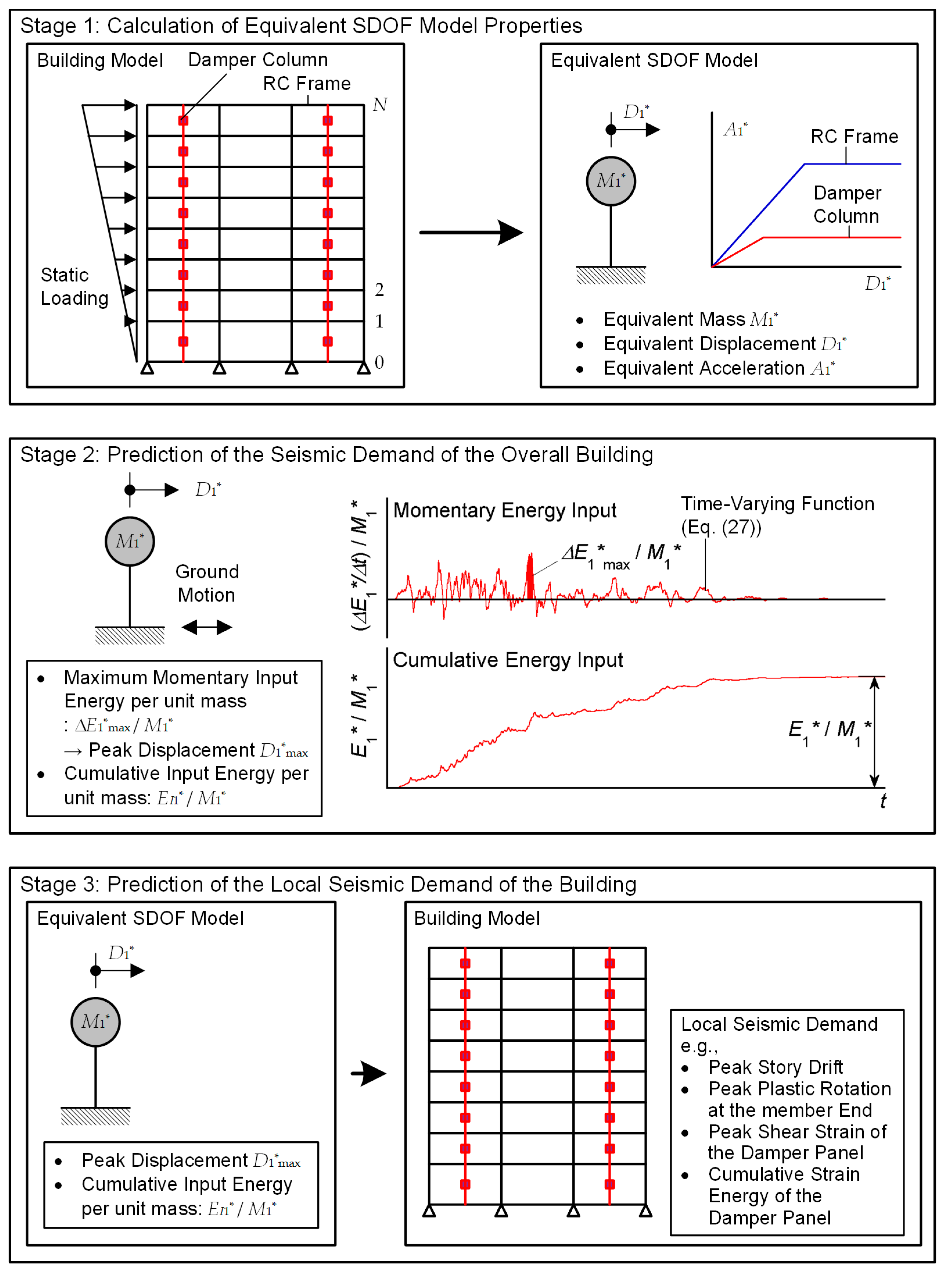
Figure 1 shows the outline of the proposed procedure.
In this procedure, the following assumptions are made.
The building oscillates predominantly in the first mode.
All RC MRFs are designed according to the strong-column/weak-beam concept, except at the foundation level beam and in the case of the steel damper columns installed in an RC frame. In the latter case, at the joints between an RC beam and a steel damper column, the RC beam is designed to be sufficiently stronger than the yield strength of the steel damper column considering strain hardening. Sufficient shear reinforcement of all RC members is provided to prevent premature shear failure. The failure of beam–column joints is not considered, as it is assumed that sufficient reinforcement is provided.
The hysteresis behavior of RC members is assumed to follow the stiffness-degrading rule, which is typical in the case of ductile RC members dominated by flexural behavior. The influences of pinching behavior [
40] and stiffness degradation after yielding as a result of cyclic loading are neglected. In addition, the hysteresis behavior of the damper panel is assumed to be elastic–perfectly-plastic. The influence of the strain-hardening effect observed in low-yield-strength steel is not considered.
The proposed procedure consists of three stages. In the first stage, the properties of the equivalent SDOF model are calculated using the pushover analysis results of the building model. The peak and cumulative responses of the equivalent SDOF model are then evaluated. In this stage, the maximum momentary input energy per unit mass (
) and the cumulative input energy per unit mass (
) are calculated based on the time-varying function of the momentary energy input, as formulated in our previous study [
28]. The peak equivalent displacement of the first modal response (
) is evaluated using
. In the third stage, the local seismic demand of the building model is predicted using the peak and cumulative response of the equivalent SDOF model (e.g.,
and
) and the results of pushover analysis.
2.1. Stage 1: Calculation of the Equivalent SDOF Model Properties
2.1.1. Stage 1-1: Pushover Analysis of the Building Model
Pushover analysis of the
-story frame building model is first carried out. The equivalent displacement and acceleration at loading step
(
and
, respectively) are calculated from Equations (1) and (2), assuming that the displacement vector at loading step
(
) is proportional to the first mode vector at loading step
(
):
In Equations (1) – (7),
is the mass of the
th floor and
is the restoring force vector at step
. The contribution of the RC MRFs and steel damper columns to the equivalent acceleration at step
(
and
, respectively) are calculated from
In Equations (8)–(11), and denote the restoring forces of the RC MRFs and steel damper columns, respectively. The restoring force vector is equal to the sum of and , which are calculated from the shear forces of the RC columns and steel damper columns, respectively.
For simplicity, the relationships between , and between , are idealized by bilinear curves, where the “yield” point of the idealized – relationship is YF (, ) and that of the idealized – relationship is YD (, ).
2.1.2. Stage 1-2: Calculation of Capacity Curve of the Equivalent SDOF Model
Next, the capacity curve of the equivalent SDOF model is calculated. In this procedure, the relation between the equivalent velocity of the maximum momentary input energy () and the equivalent displacement is referred to as the capacity curve.
The energy dissipated in half a cycle per unit mass of the equivalent SDOF model (
) is calculated as
In Equation (12), and are the contributions from the hysteretic dissipated energies of the RC MRFs and steel damper columns, respectively, while is the contribution from viscous damping.
The contribution from the hysteretic dissipated energy of the RC MRFs is calculated as
In Equations (13)–(15),
is the global ductility of the RC MRFs. The contribution from the hysteretic dissipated energy of the steel damper columns is calculated as
In Equations (16)–(18),
is the global ductility of the steel damper columns. The contribution from viscous damping is calculated as
where
is the viscous damping ratio of the RC MRFs of the first modal response in the elastic range. The formulation of Equations (12)–(20) is described in
Appendix A.
The equivalent velocity of the maximum momentary input energy corresponding to
(
) is calculated as
The effective period of the first modal response at step
(
) is calculated as
where
is the complex damping ratio of the equivalent linear system considered for the calculation of the
and
spectra. The formulation of Equation (22) is described in
Appendix B.
2.2. Stage 2: Prediction of the Seismic Demand of the Overall Building
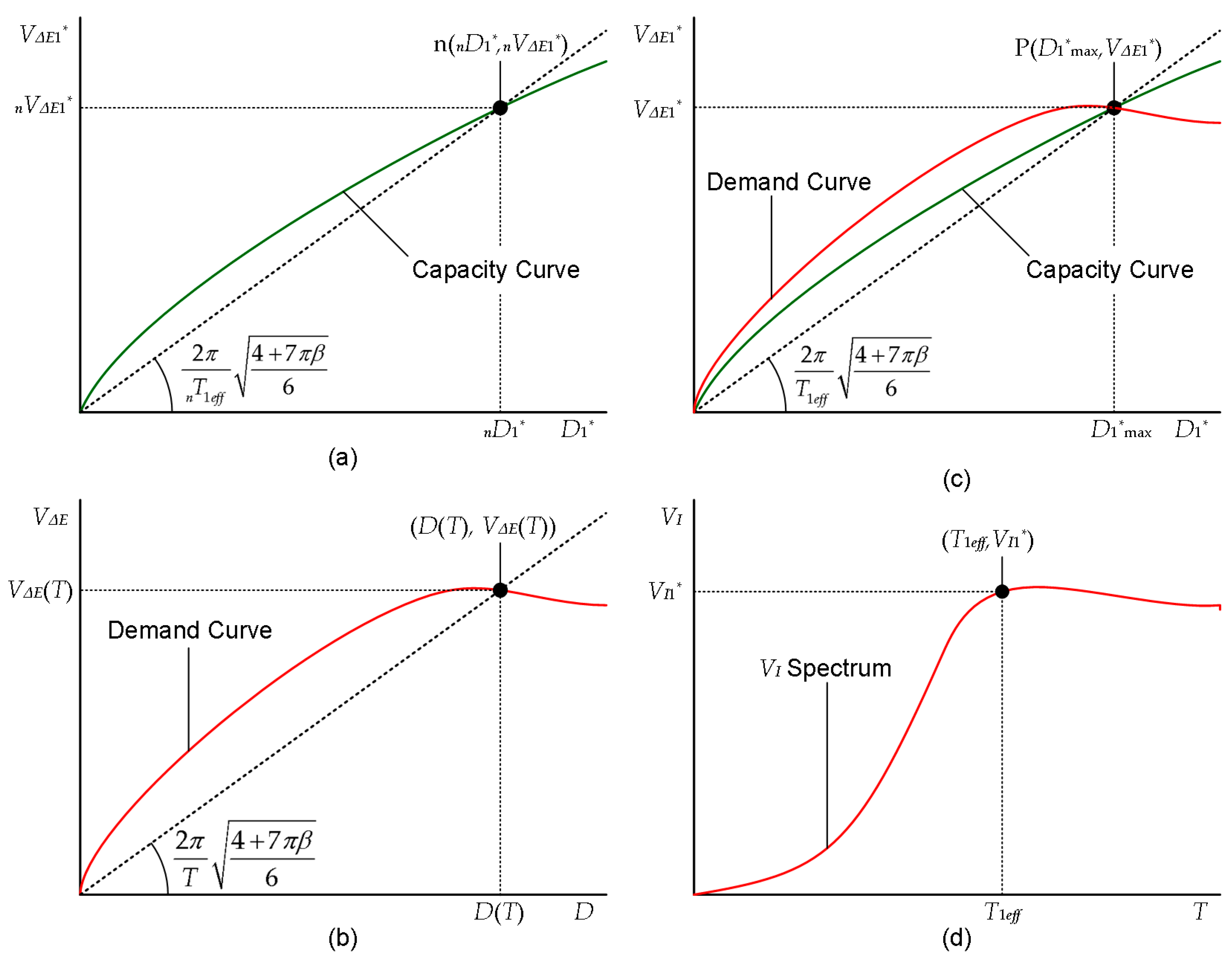
The schemes for predicting the peak and cumulative responses of the equivalent SDOF model are shown in
Figure 2.
The capacity curve obtained in stage 1 is shown in
Figure 2(a): the secant slope of the capacity curve at point
n (
,
) corresponds to the effective period of the equivalent SDOF model (
). The demand curve (
–
relationship) shown in
Figure 2(b) is calculated in stages 2-1 and 2-2. The peak response point P (
,
) is at the intersection of the capacity and demand curves, as shown in
Figure 2(c). The velocity of the cumulative input energy in the equivalent SDOF model (
) is obtained from the
spectrum calculated in stage 2-1 and the effective period, corresponding to point P (
), as shown in
Figure 2(d).
2.2.1. Stage 2-1: Calculation of and Spectra
The
and
spectra are calculated from the time-varying function proposed in our previous study [
28]. A discrete time history of the ground motion (
), defined within the range
, can be expressed as
where
and
( =
) are the complex Fourier coefficients of the ground motion and the circular frequency of the
th harmonic, and
is the imaginary unit. The coefficient
is assumed to be zero. For a given natural period
and complex damping ratio
, the displacement and velocity transfer function of the equivalent linear system is calculated as
In Equation (24),
(
) is the natural circular frequency of the equivalent linear system. The duration of a half cycle of the response (
) is calculated as
The time-varying function of the momentary energy input can then be calculated as
In Equation (28), the overbar indicates the complex conjugate. Note that the time-varying function in Equation (27) is shown in the middle of
Figure 1. The momentary input energy per unit mass at time
is calculated as
The maximum momentary input energy per unit mass (
) can be evaluated as the maximum value calculated by Equation (29) over the course of the seismic event. The total input energy per unit mass (
) can be calculated as
The equivalent velocities of the maximum momentary input energy (
) and the total input energy (
) are calculated as
2.2.2. Stage 2-2: Calculation of Demand Curve
The demand curve (
Figure 2(b)) is calculated from the
spectrum as follows. The equivalent displacement of the equivalent linear system (natural period
, complex damping ratio
) is calculated as
2.2.3. Stage 2-3: Determination of the Peak and Cumulative Response of the Equivalent SDOF Model
The peak response point P is shown in
Figure 2(c): in this figure, the peak response point P (
,
) is obtained as the intersection of the capacity curve and the demand curve. The effective period corresponding to point P is then calculated as
2.2.4. Stage 2-4: Calculation of the Cumulative Energies of the Overall Building
The equivalent velocity of the cumulative input energy of the first modal response (
) is obtained from the
spectrum as
The cumulative dissipated energy of the equivalent SDOF model is calculated as follows. The cumulative input energy of the first modal response per unit mass (
) is calculated as
where
is the effective first modal mass corresponding to the peak response point and
is the total mass. Note that
is factored by
. This is because the total input energy of the whole building is greater than the cumulative input energy of the first modal response. Therefore, in this study,
is factored by the ratio
to give a conservative prediction of the cumulative dissipated energy.
The cumulative strain energies of RC MRFs and steel damper columns are calculated as follows. The ductility factors of RC MRFs and steel damper columns (
and
, respectively) are given by
Next, the dissipated strain energy of RC MRFs per unit mass under monotonic loading (
) and under cyclic loading (
) are calculated as
Similarly, the dissipated strain energy of the steel damper columns per unit mass under monotonic loading (
) and under cyclic loading (
) are calculated as
The dissipated damping energy per unit mass over each cycle of the structural response (
) is calculated as
In Equation (43),
is the loading step of pushover analysis, corresponding to the peak equivalent displacement
. The formulation of Equations (38)–(44) is given in
Appendix C.
From the energy balance of the cumulative energy in the whole seismic event, the equivalent number of cycles
is calculated as
From
, the cumulative strain energies of RC MRFs and steel damper columns over the whole seismic event (
and
, respectively) are calculated as
2.3. Stage 3: Prediction of the Local Seismic Demand of the Building Model
2.3.1. Stage 3-1: Determination of Peak Local Seismic Demand
Pushover analysis is applied until the equivalent displacement reaches the peak equivalent displacement obtained in stage 2-3 (). The peak local seismic demand (e.g., relative displacement, story drift, plastic rotation of member ends, strain energy of dampers) is obtained as a quantity corresponding to .
2.3.2. Stage 3-2: Calculation of Cumulative Response Demand of each Damper Column
The cumulative strain energy of a damper panel (
) is calculated as
In Equations (49) and (50), , , , and denote the ductility, peak shear strain, initial yield shear strain, and height of the th damper panel, respectively. In this study, for simplicity, is assumed to be proportional to the average dissipated strain energy under cyclic loading ().
The cumulative strain energy of a damper panel (
) is normalized as follows for simplicity:
In this version of the procedure, the cumulative response demand of each RC member is not calculated. Elwood et al. have studied the impact of prior shaking on the earthquake response and repair requirements of ductile RC MRFs [
41]. They concluded that simple (or no) repairs are sufficient provided that the story drift did not exceed 2.0% because “cyclic loading up to 2% drift had a limited impact on the deformation capacity of column specimens with up to 0.1 axial load ratio” [
41]. Therefore, for ductile RC members, the prediction of the peak response demand is sufficient unless the story drift exceeds 2.0%.
3. Model Structures and Ground Motions
3.1. Model Structures
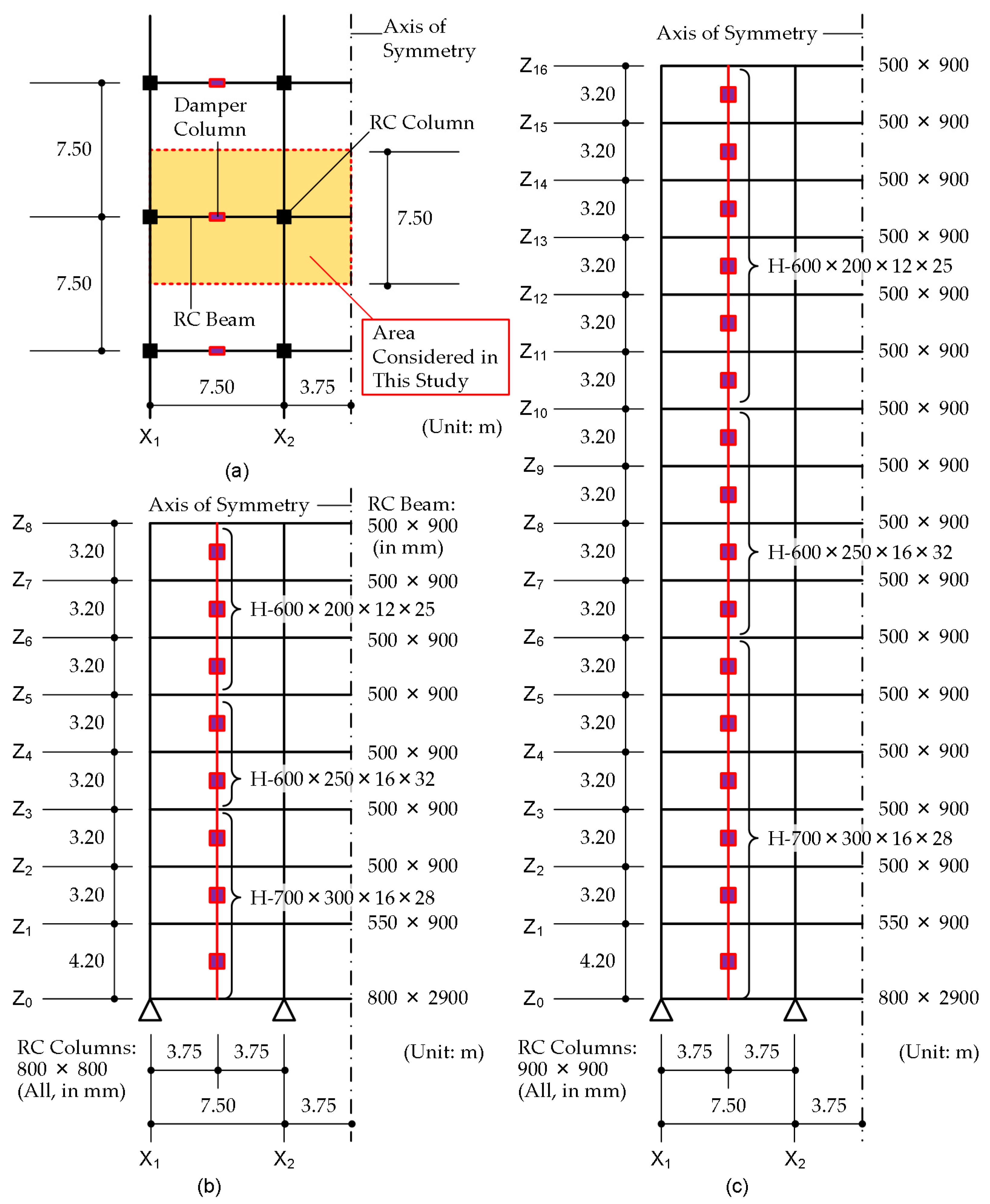
Figure 3 shows a simplified structural plan and elevation of the MRF building models with steel damper columns considered in this study. Eight- and 16-story building models are designed using the simplified procedure [
5]. In the seismic design of these two frames, the displacement limit
is assumed to be 1/75 of the equivalent height:
is 0.252 m for the 8-story model and 0.479 m for the 16-story model. Both models have the same structural plan. The unit mass per floor is assumed to be 1.2 t/m
2. The story height is assumed to be 4.2 m for the first story and 3.2 m for upper stories. Details of the members are given in
Appendix D.
All MRFs are modeled as planar frames: the MRF with steel damper columns is modeled as in previous studies [
5,
7]. In this study, only half of the frame is modeled considering the symmetry of the structure. All RC members are modeled as elastic beams with nonlinear flexural springs at both ends. The steel damper columns are modeled as elastic columns with nonlinear damper panels in the middle. The beam–column joints are assumed to exhibit rigid behavior. For RC beam–RC column joints, it is assumed that proper reinforcement is provided to prevent premature failure. In addition, appropriate dimensions of the steel beam embedded in the RC beams and suitable reinforcement are assumed in the RC beam–damper column joints, to prevent premature failure until the damper panels reach their ultimate stage.
The nonlinear behavior of the RC members and steel damper columns is modeled as in previous studies [
5,
7]. The envelope of the force–deformation relationship at the potential hinge of the RC members is modeled as a trilinear curve, considering the cracking and yielding of the section. The non-hinges of RC members are modeled as bilinear curves, considering only the cracking of the section. The behavior of the beam at the foundation level is assumed to be linearly elastic. The same hysteresis model (stiffness degradation model) is used for the flexural springs in the RC members. Pinching behavior is not considered in this study. The shear behavior of RC members is assumed to be linearly elastic. The axial force–moment interaction of the columns is not considered for simplicity. Similarly, the same hysteresis model (normal bilinear model neglecting the strain-hardening effect for pushover analysis, trilinear model with strain-hardening effect for nonlinear time-history analysis) is used for the damper panels. Details of the modeling can be found in previous studies [
5,
7]. For simplicity, the stiffness degradation of RC members after yielding under cyclic loading, which was considered in a previous study [
7], is not considered in this paper.
Table 1 presents the natural periods of the first three modes in the initial stage for each model. The natural period of the 16-story model is longer than that of the 8-story model.
In this study, the damping matrix is assumed to be proportional to the tangential stiffness of the RC MRFs.
3.2. Ground Motions
Two groups of artificial ground motions are generated. The target spectrum is the code-specific spectrum (soil condition: type-2 (normal)) of the Building Standard Law of Japan [
42], defined as
The phase angle is given by a uniform random value. To consider the time-dependent amplitude of the ground motions, a Jenning-type envelope function (
) is assumed. In this study, two envelope functions are considered. In Art-L-00, the envelope function is set as in Equation (53), whereas in Art-S-00, the envelope function is set as in Equation (54).
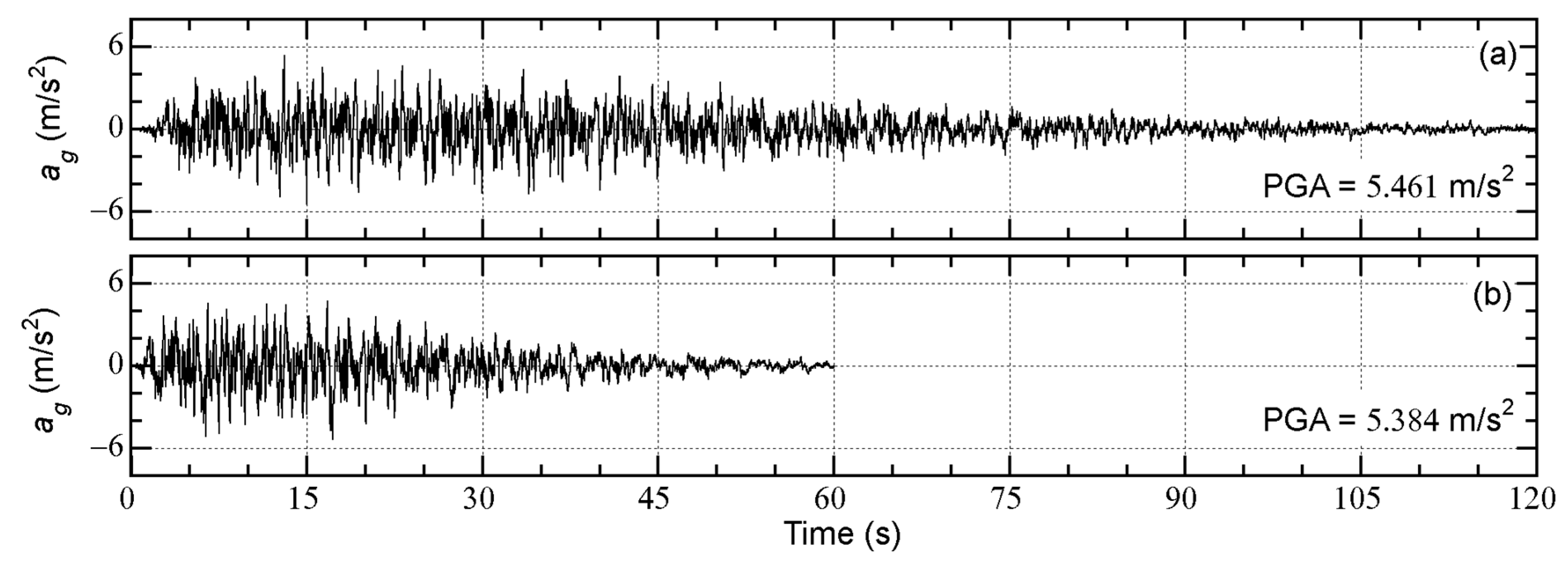
Figure 4 shows the time histories of the artificial ground accelerations of Art-L-00 and Art-S-00, respectively.
Eleven artificial ground motions are generated from Art-L-00 and Art-S-00 by shifting the phase angle. The generated artificial ground motion
is expressed as
where
is the constant used to shift the phase angle of all harmonics. As in previous studies [
28,
30,
31],
varies from
to
at intervals of
. The generated artificial ground motions are numbered from 01 to 11 accordingly. A total of 2 × 12 = 24 artificial ground motions are used in this study.
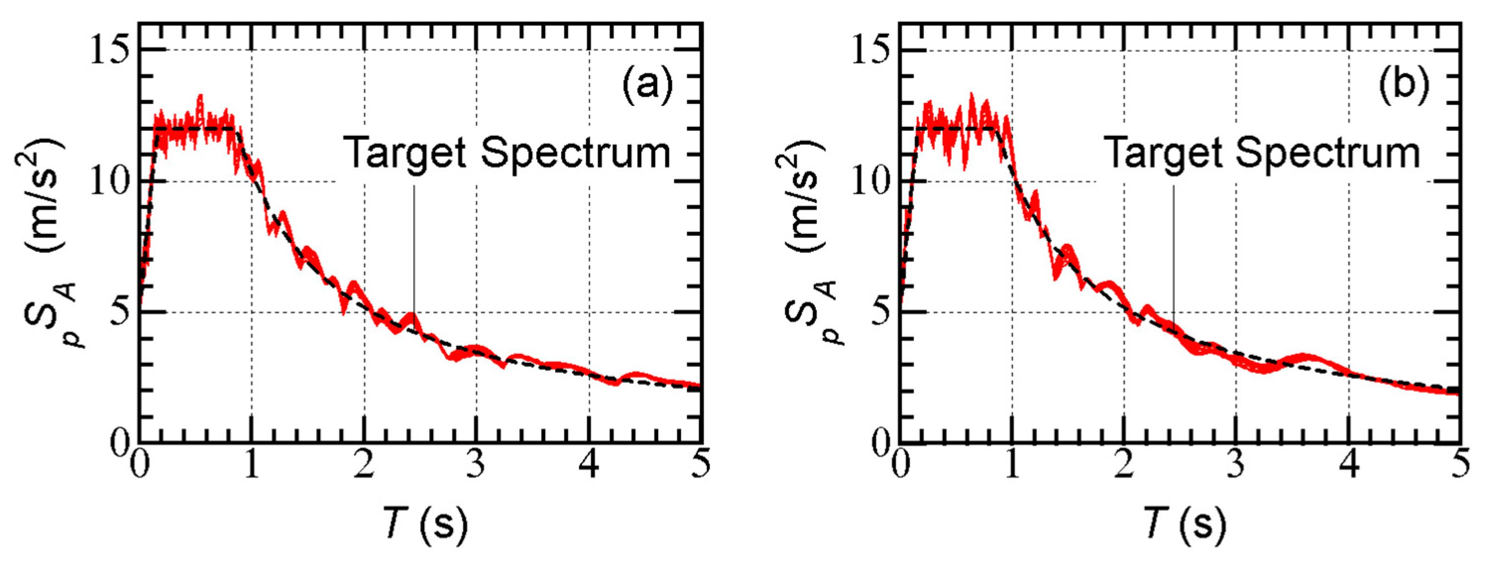
Figure 5 shows the elastic pseudo-acceleration spectra (damping ratio: 0.05) of the generated ground motions. As shown in this figure, the difference in
caused by changes in the phase angle is very limited.
3.3. Analysis Cases
The following parameters are considered for the validation of the proposed procedure.
The complex damping ratio of the equivalent linear system (): the complex damping ratio of the equivalent linear system is the key parameter in obtaining better predictions of the energy response. Therefore, three different values of are considered: 0.05, 0.10, and 0.15.
The viscous damping ratio of the first modal response of RC MRFs in the elastic range (): the accuracy of the cumulative energy depends on the viscous damping of the RC MRFs. Therefore, three different values of are considered: 0.00, 0.03, and 0.05.
4. Analysis Results
In
Section 4.1, the process of predicting the seismic demand of the overall building using the equivalent SDOF model is presented. The predicted results are then compared with the nonlinear time-history analysis results of frame models in
Section 4.2.
4.1. Prediction of the Seismic Demand of the Equivalent SDOF Model
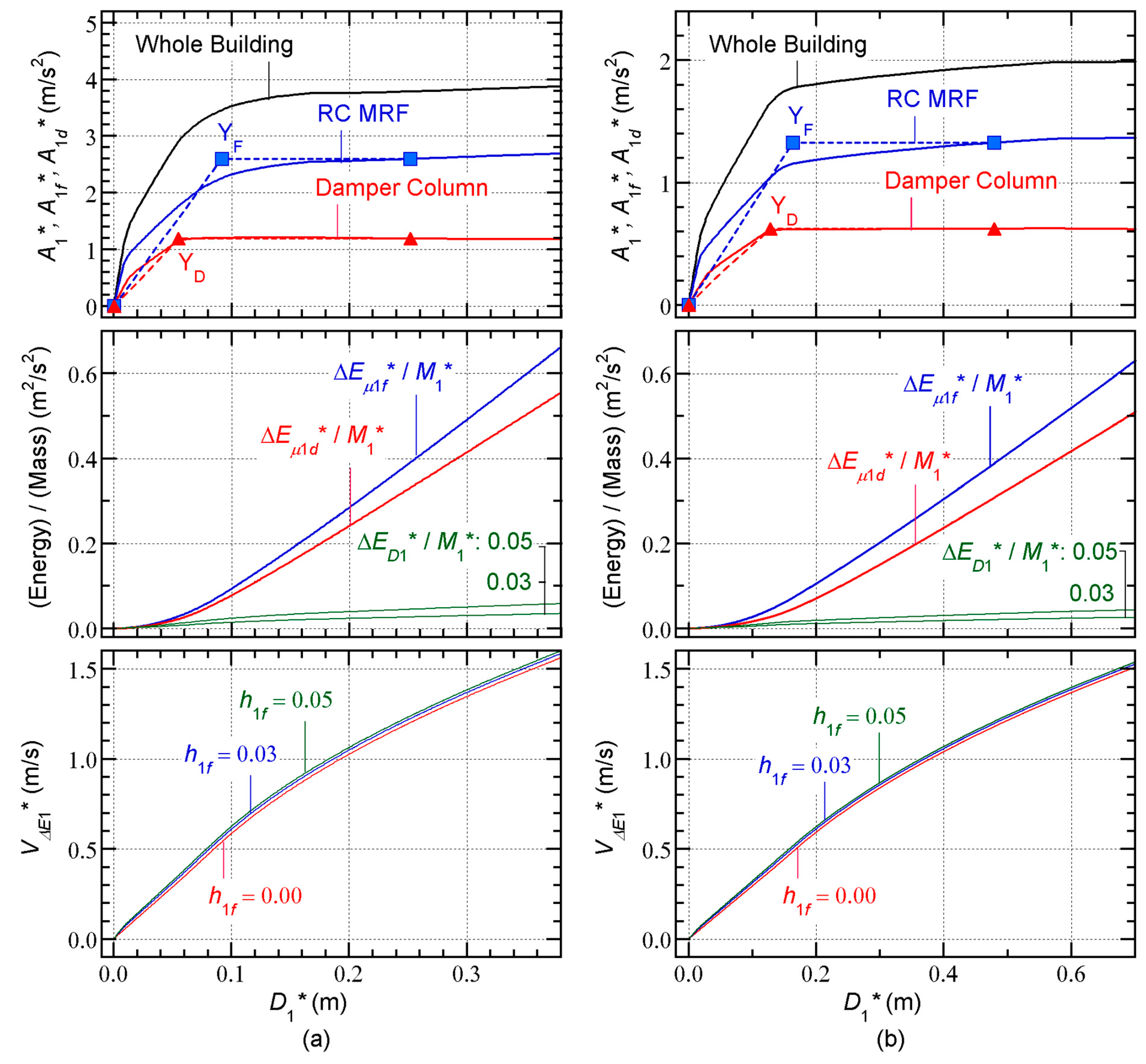
Figure 6 shows the capacity curve of the building models (stage 1 in
Figure 1). The calculation results for the 8-story model are shown in
Figure 6(a), whereas those for the 16-story model are shown in
Figure 6(b). In this study, displacement-based mode-adaptive pushover analysis [
43] is applied to obtain the relationship between the equivalent acceleration (whole building:
, RC MRF:
, and damper column:
) and equivalent displacement
. The
–
and
–
relationships are idealized as bilinear curves following a previous study [
7].
The dissipated energy in a half cycle per unit mass of the equivalent SDOF model is calculated according to the procedure described in
Section 2.1.2. The calculated results are shown in the middle part of
Figure 6. The contribution of the RC MRFs (
) is calculated using Equations (13)–(15). The contribution from the steel damper columns (
) is calculated using Equations (16)–(18). The contribution of viscous damping (
) is calculated from Equations (19) and (20). Note that the calculated
depends on the viscous damping ratio of the first modal response of RC MRFs in the elastic range (
):
for
= 0.00 is not shown because
is zero in this case.
The calculated capacity curves (
–
relationship) are shown at the bottom of
Figure 6. In this figure, the difference in the capacity curves as
varies is almost negligible.
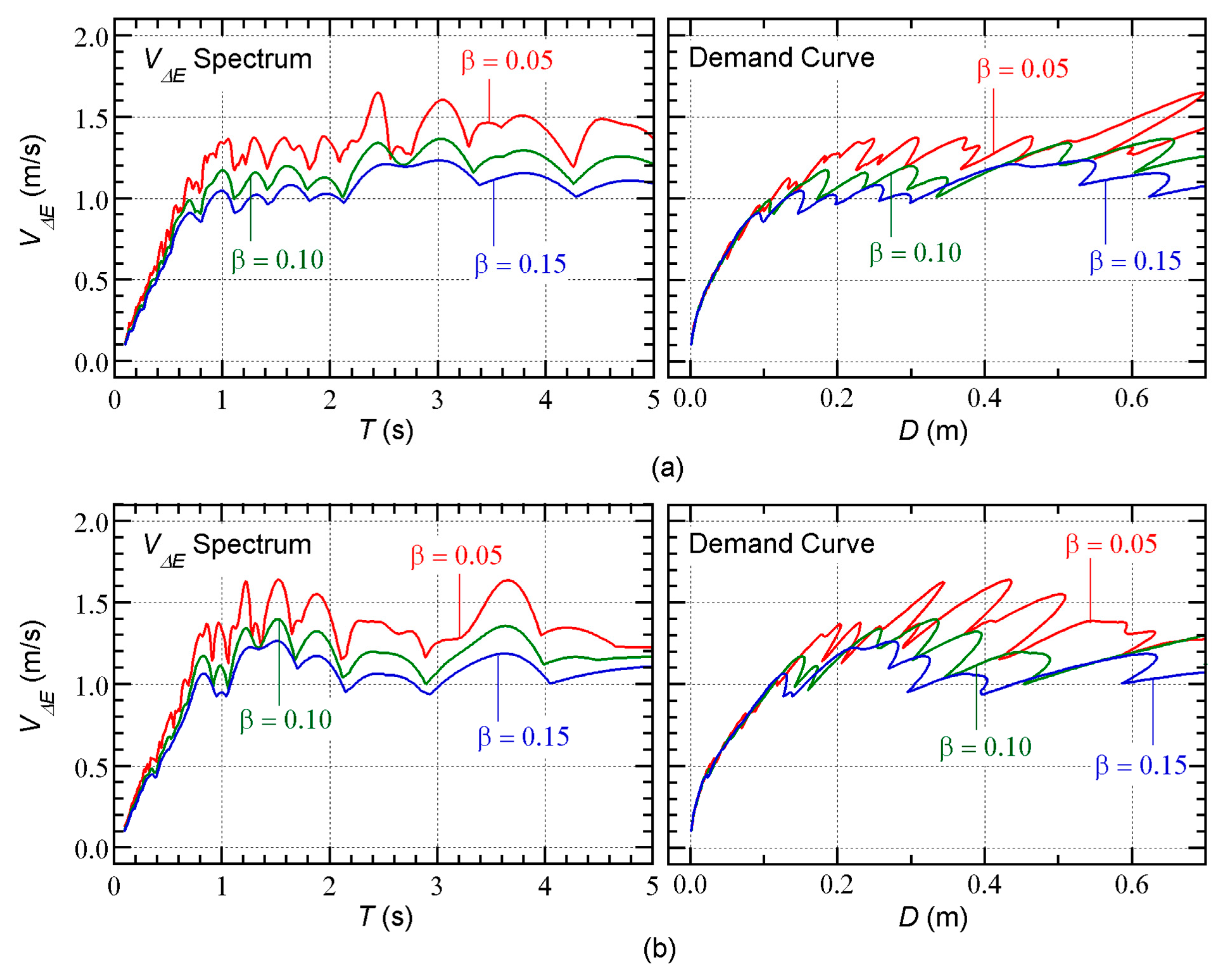
Figure 7 shows the calculated
spectrum and demand curve (
–
relationship). The
spectrum calculated using the time-varying function in Equation (27) is independent of the phase shift
, as described in previous studies [
28,
30].
Figure 7(a) shows the results calculated from the Art-L series, whereas
Figure 7(b) shows the results for the Art-S series.
On the left of
Figure 7(a), the calculated
spectrum is largest when
= 0.05 and smallest when
= 0.15. The demand curves are compared on the right of
Figure 7(a). The three demand curves are almost identical when
is less than 0.9 m/s. Similar observations can be made for the Art-S series in
Figure 7(b).
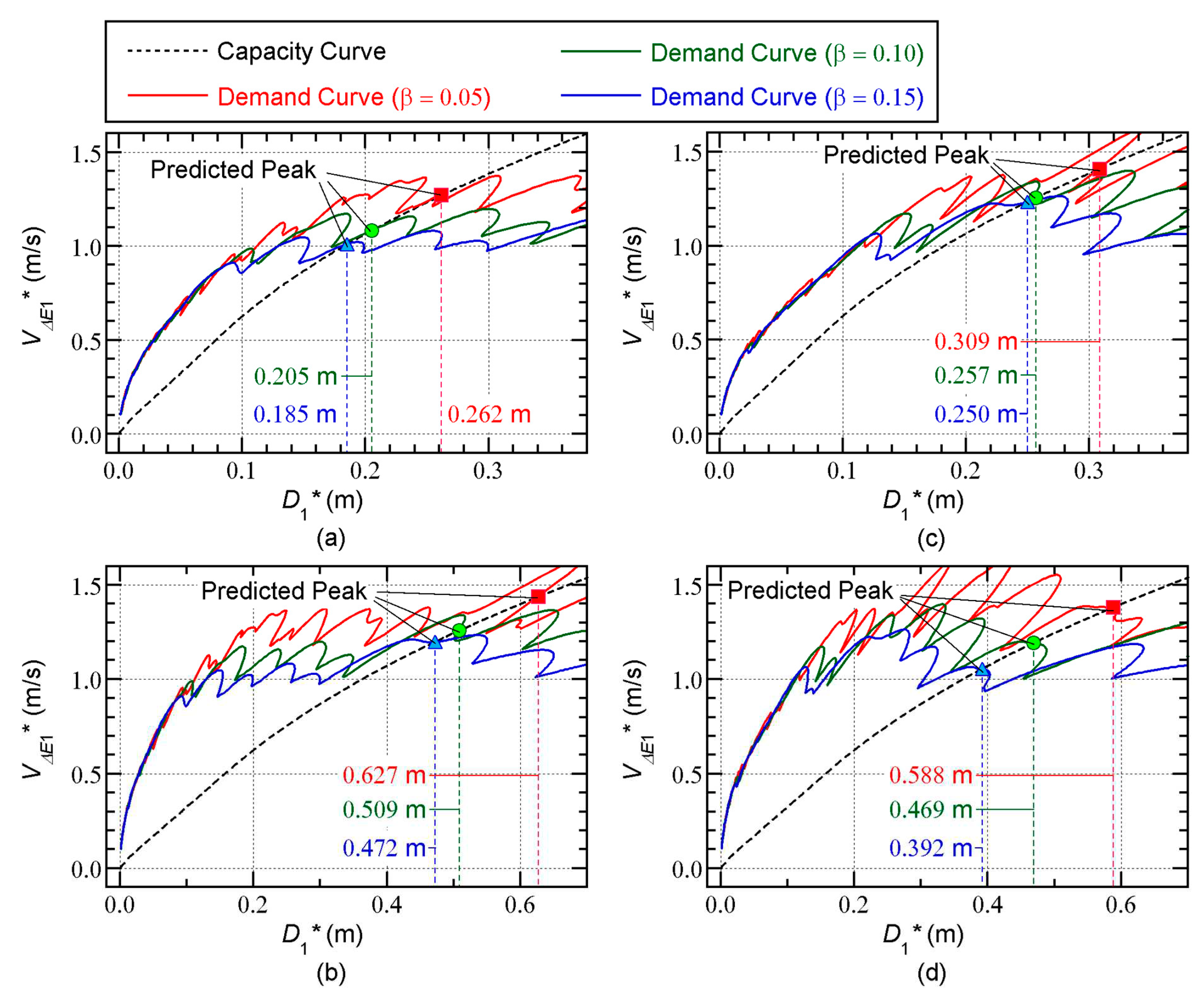
Figure 8 shows the predicted peak response points for each model using the three demand curves. In this figure, the predicted results are presented for
= 0.05. As described in
Section 2.2.3, the intersection of the capacity and demand curves is the predicted peak response point.
In
Figure 8(a), the largest equivalent displacement (
) occurs when
= 0.05, while the smallest
is obtained with
= 0.15. Similar observations can be made in
Figure 8(b)–(d). Note that the difference in the predicted
for the Art-L and Art-S series depends on the model: a comparison of
Figure 8(a) and
Figure 8(c) indicates that the predicted
for the Art-L series is larger than that for the Art-S series in the case of the 8-story model, while the opposite conclusion can be reached for the 16-story model.
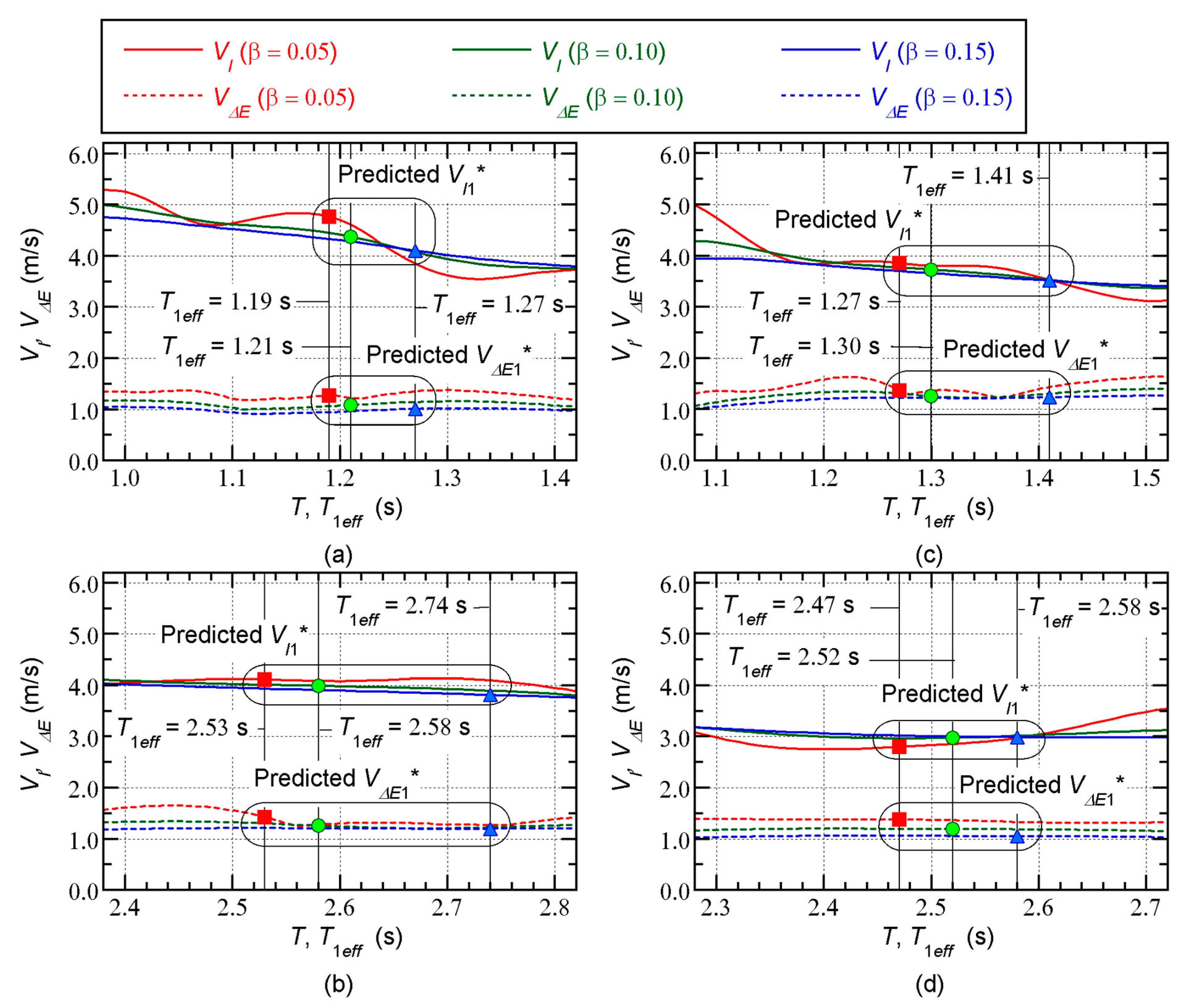
Figure 9 shows the predicted equivalent velocity of the cumulative input energy for the first modal response. The predictions shown in this figure are for
= 0.05. The spectra for both
and
are shown. The vertical lines indicate the effective period (
) at the predicted peak response point. The predicted equivalent velocity (
) is obtained as the intersection of the
spectra and the vertical lines.
A comparison of
Figure 9(a) and
Figure 9(c) indicates that the predicted
for the Art-L series is larger than that for the Art-S series in the case of the 8-story model. The same conclusion can be obtained for the 16-story model by comparing
Figure 9(b) and
Figure 9(d).
4.2. Comparisons with the Time-History Analysis Results
In this section, the predicted seismic demands are compared with the nonlinear time-history analysis results.
4.2.1. Energy Demand of the Overall Building
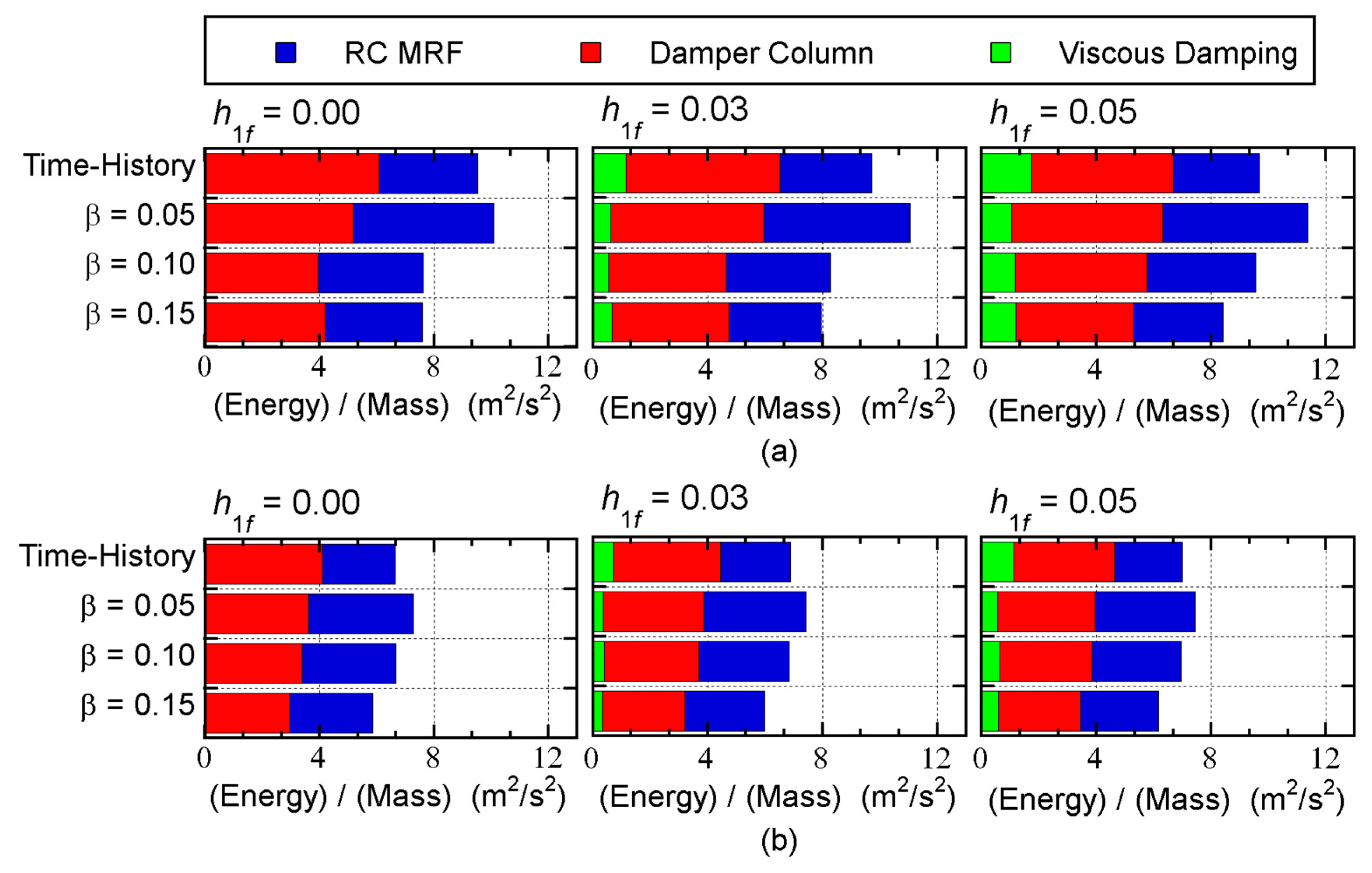
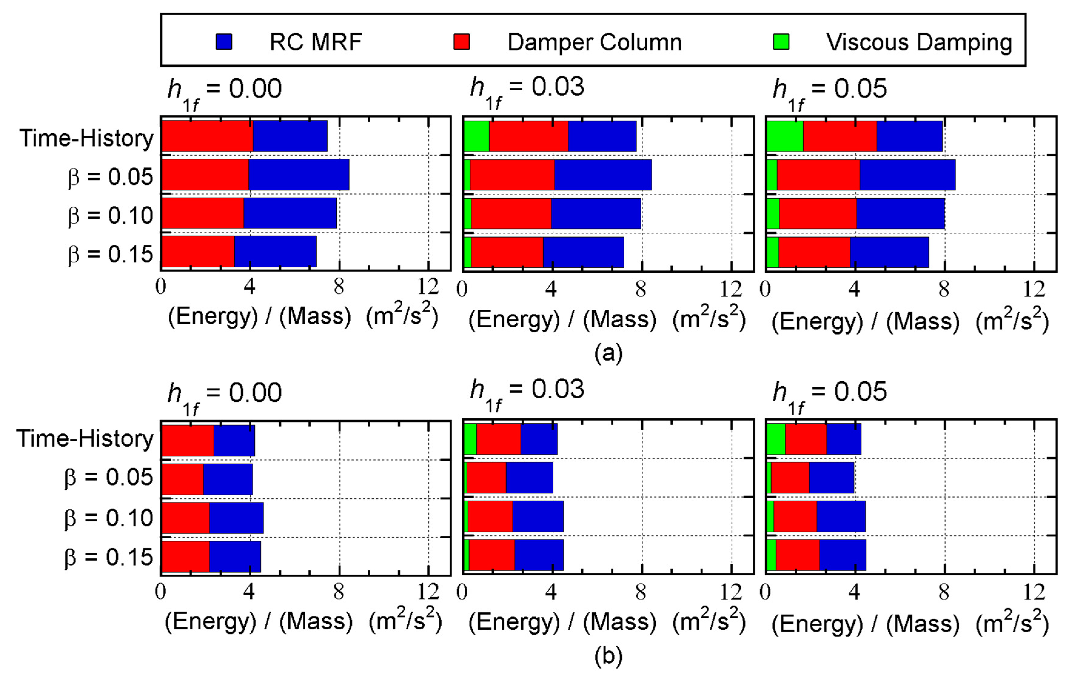
Figure 10 and
Figure 11 compare the predicted energy demand of the overall building with the nonlinear time-history analysis results. These figures show the mean nonlinear time-history analysis results. All quantities have been normalized by the total mass
. In addition, the total input energy is the sum of the cumulative strain energies of RC MRF and damper columns, and the cumulative energy of viscous damping.
The following observations can be made for these figures.
For the 8-story model shown in
Figure 10, the relationships between the predicted total input energies and the nonlinear time-history analysis results depend on the ground motion series and the value of
: the predicted total input energy with
= 0.15 is unconservative for all cases. For the 16-story building model shown in
Figure 11, the predicted total input energy agrees well with that obtained from the nonlinear time-history analysis results for all cases.
The predicted cumulative strain energy of the RC MRFs is larger than that obtained from the nonlinear time-history analysis results for both models.
The predicted cumulative strain energy of the steel damper columns is close to that of the nonlinear time-history analysis results for both models.
The predicted cumulative energy of viscous damping is smaller than that of the nonlinear time-history analysis results, except when = 0.00.
Therefore, we believe that the predicted energy demand of the whole building is acceptable, although the predicted cumulative energy of viscous damping is small. Considering the energy balance of the whole seismic event, smaller predicted values of the energy of viscous damping lead to larger (more conservative) predictions of the strain energy demands of RC MRFs and damper columns. In addition, the contribution of viscous damping to the whole energy response is small, as shown in
Figure 10 and
Figure 11. Therefore, smaller predicted values of the viscous damping energy will not be critical.
4.2.2. Local Seismic Demand
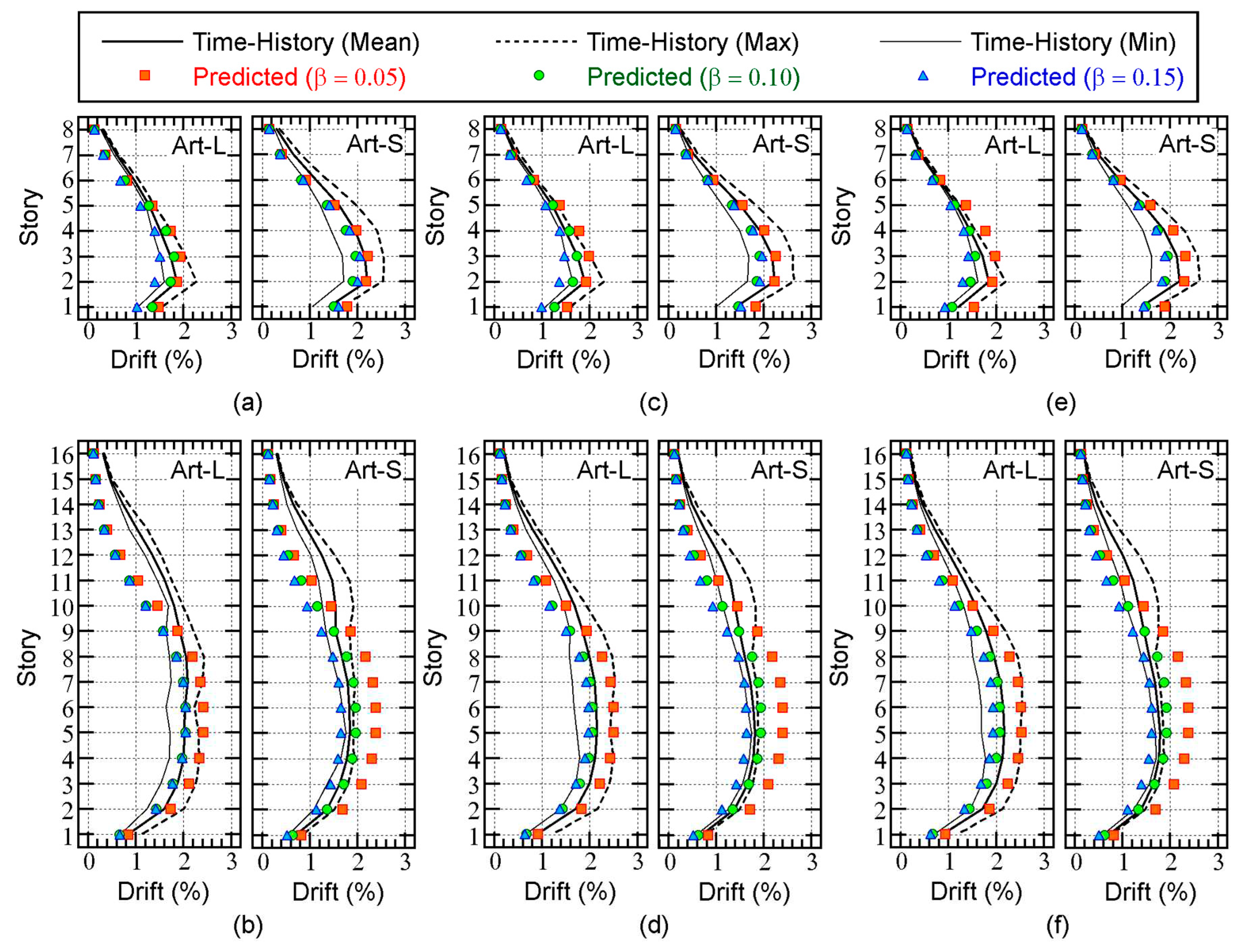
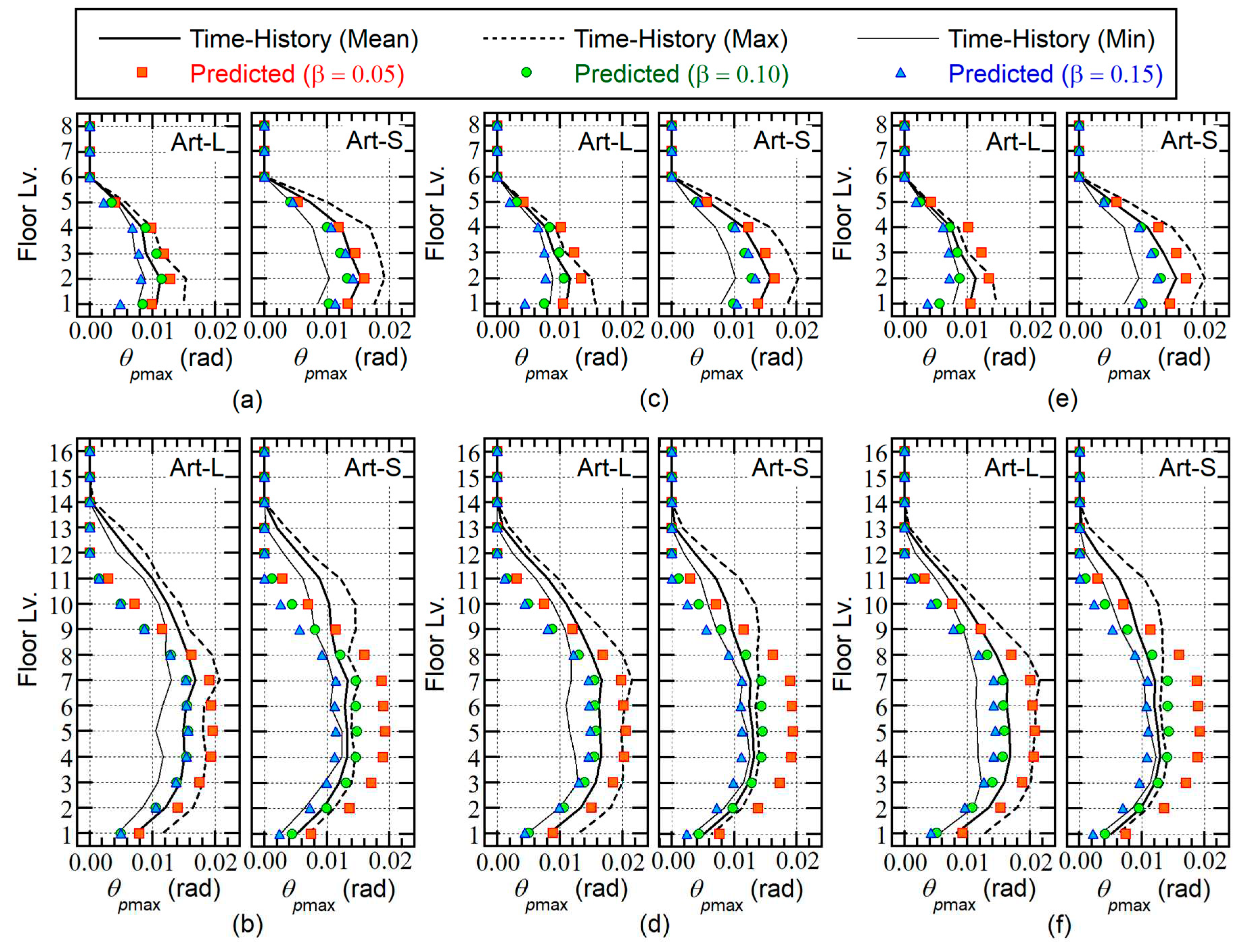
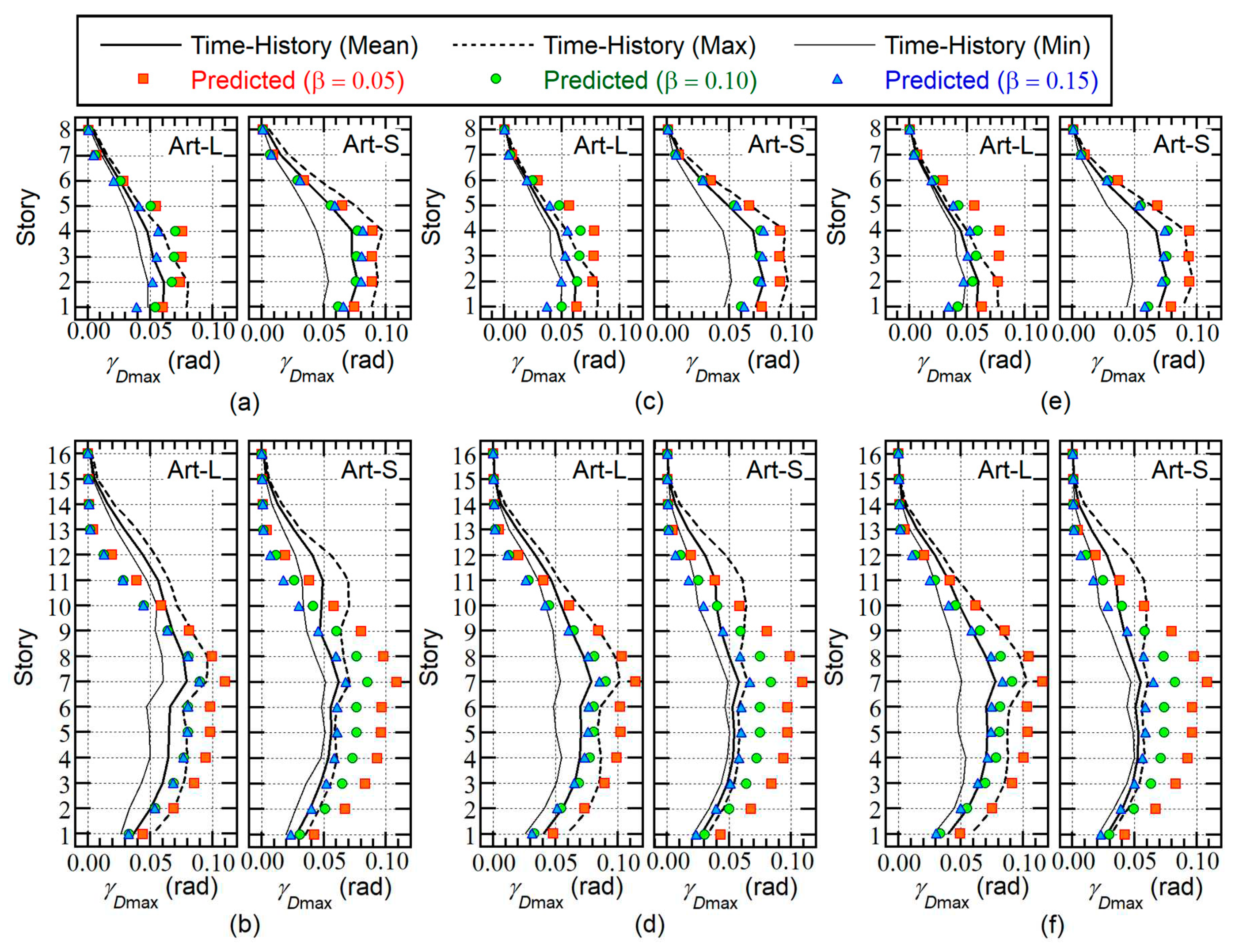
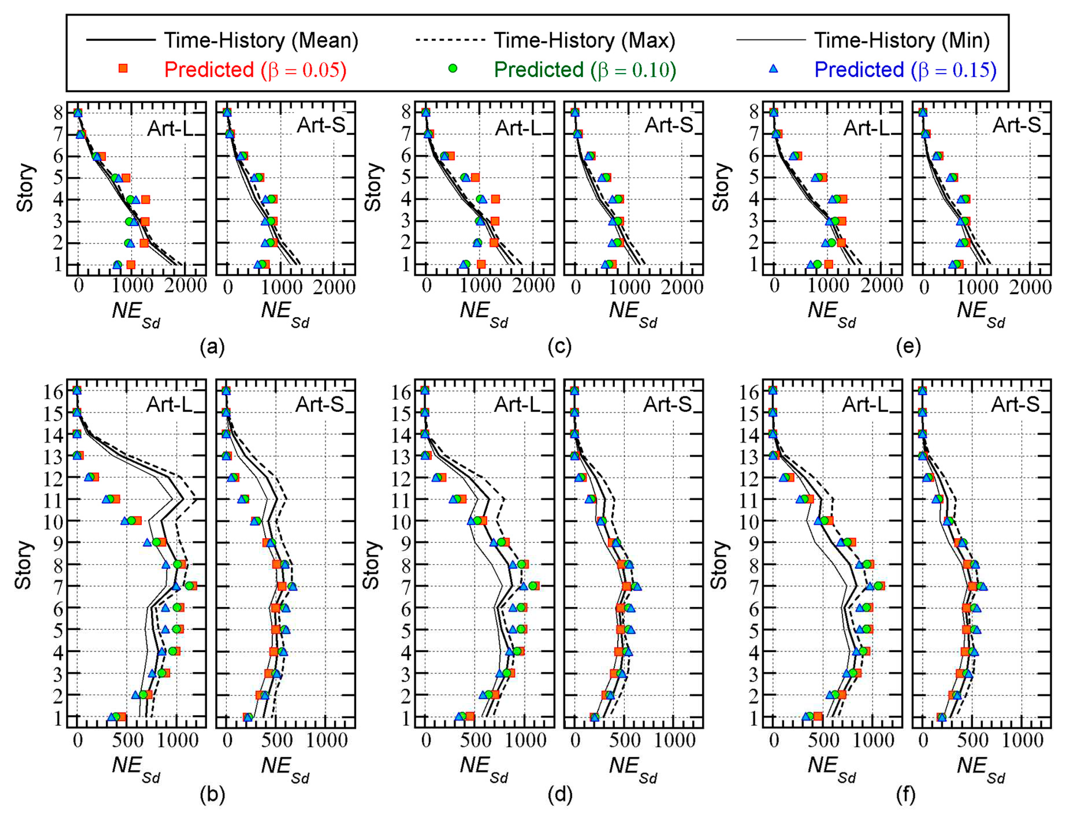
In this section, the following local response quantities are compared: (i) peak story drift, (ii) peak plastic rotation at the beam end, (iii) peak shear strain of the damper panels, and (iv) normalized cumulative strain energy of the damper panels. The mean, maximum, and minimum values of the nonlinear time-history analysis results for the 12 ground motions are compared with the predicted results.
Figure 12 compares the predicted peak story drift with the nonlinear time-history analysis results for the Art-L and Art-S ground motion series.
The following observations can be made for
Figure 12.
For the 8-story model, the predicted peak drift with = 0.05 is larger than the mean of the nonlinear time-history analysis results, whereas the predicted peak drift with = 0.10 is slightly smaller than the mean of the nonlinear time-history analysis results. When = 0.15, the predicted peak drift is smaller than the mean of the nonlinear time-history analysis results.
For the 16-story model, the predicted peak story drift with = 0.10 is in good agreement with the nonlinear time-history analysis results below the mid-story level (7th or 8th story). However, the predicted peak story drift above this level is lower than the nonlinear time-history analysis results. This tendency is noticeable when = 0.00.
Figure 13 compares the predicted peak plastic hinge rotation at the beam end (
) with the nonlinear time-history analysis results. This figure shows
for the beam end at the right of column X2.
The following observations can be made for
Figure 13.
For the 8-story model, the predicted with = 0.05 is slightly larger than the mean of the nonlinear time-history analysis results. The predicted are unconservative when = 0.10 or = 0.15.
For the 16-story model, the predicted with = 0.05 is too conservative below the mid-story level (7th or 8th story). The predicted with = 0.10 agrees well with the mean of the nonlinear time-history analysis results below the mid-story level. For = 0.15, the predicted is unconservative at all floors.
Figure 14 compares the predicted peak shear strain of the damper panels (
) with the nonlinear time-history analysis results. The following observations can be made for
Figure 14.
For the 8-story model, the predicted with = 0.05 is larger than the mean of the nonlinear time-history analysis results. The predicted for the cases where = 0.10 and = 0.15 are closer to the mean of the nonlinear time-history analysis results.
For the 16-story model, the predicted with = 0.05 is too conservative below the mid-story level (9th or 10th story). The predicted when = 0.10 is also conservative below the mid-story level, but is closer to the mean of the nonlinear time-history analysis results. The predicted with = 0.15 is the closest to the mean of the nonlinear time-history analysis results.
Figure 15 compares the predicted normalized cumulative strain energy of the damper panels (
) with the nonlinear time-history analysis results. The following observations can be made for
Figure 15.
For the 8-story model, the predicted is larger than that of the nonlinear time-history analysis results above the 2nd story. However, the predicted at the 1st story underestimates the nonlinear time-history analysis results.
For the 16-story building model, the predicted is in good agreement with the nonlinear analysis results below the mid-story level (9th or 10th story). However, the predicted above the mid-story level underestimates the nonlinear time-history analysis results. This is noticeable when = 0.00.
4.3. Summary of the Analysis Results
This section has demonstrated the procedure for predicting the seismic demand of the equivalent SDOF model. The predicted seismic demands were then compared with the nonlinear time-history analysis results. The analysis results can be summarized as follows.
The accuracy of the predicted energy demand of the whole building is acceptable, although the predicted cumulative energy of viscous damping is small.
The accuracy of the predicted local peak seismic demands (story drift, plastic rotation of the beam end, and shear strain of the damper panels) is acceptable, although some quantities are unconservative.
The accuracy of the predicted cumulative energy strain energy demand of the damper panels is acceptable, although some values are unconservative.
It is important to mention that the underestimations of the local seismic demand observed at some points occur because of higher modal responses: in this procedure, only the contribution of the first modal response is considered.
5. Discussion
The accuracy of the proposed procedure strongly relies on the prediction of the seismic demand of the equivalent SDOF model in stage 2 (
Figure 1). In this section, the discussion focuses on (i) the applicability of the time-varying function of the momentary energy input for predicting the energy response and (ii) the relationship between the peak equivalent displacement and the maximum momentary input energy of the first modal response. The equivalent velocities of the maximum momentary input energy and the cumulative energy (
and
), and the peak equivalent displacement
, are calculated from the nonlinear time-history analysis results according to the procedure presented in a previous study [
7].
5.1. Applicability of the Time-Varying Function of the Momentary Energy Input for Predicting the Energy Response
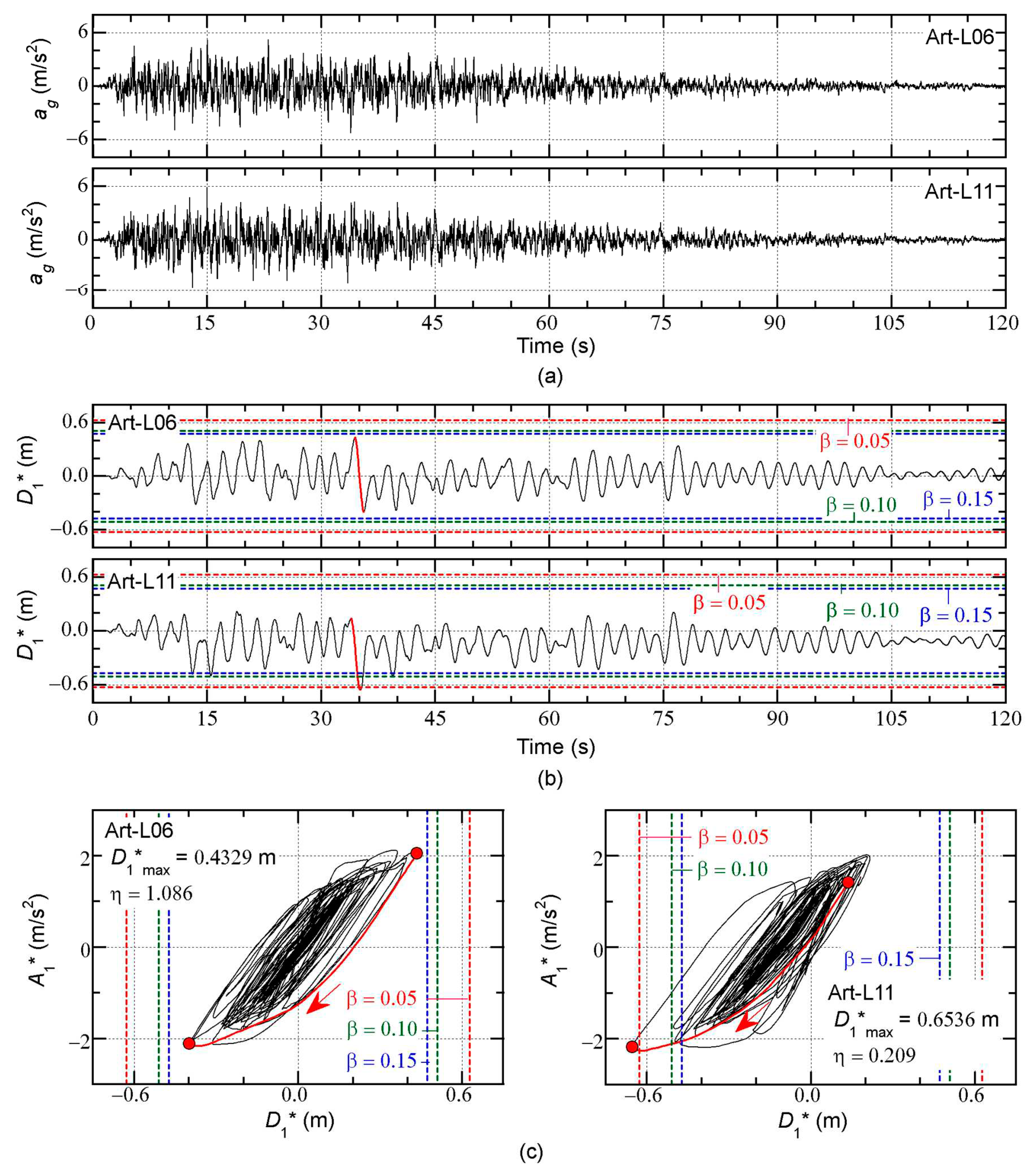
Figure 16 shows the time-history and hysteresis of the first modal response of the 16-story model as an example. In this figure, the results obtained with
= 0.05 are shown for the Art-L-06 and Art-L-11 ground accelerations. The dashed lines in
Figure 16(b) indicate the predicted peak equivalent displacement (
) for three values of
. In
Figure 16(c),
is the ratio of the local peak equivalent displacement (in the positive and negative directions), defined as
where
and
are the start and end times, respectively, of the half cycle when the maximum momentary input energy of the first modal response (
) occurs. The time-history and the hysteresis loop during the half cycle (from
to
) are denoted by the red curves.
The following observations can be made for
Figure 16.
Although the time-histories of ground accelerations are very similar, the time-histories of the equivalent displacement are different. The equivalent displacement does not exceed the predicted in the case of Art-L-06, but does exceed the predicted in the case of Art-L-11.
The hysteresis loop is almost symmetric in the case of Art-L-06 (left of
Figure 16(c)), but is notably asymmetric in the case of Art-L-11 (right of
Figure 16(c)). The ratio
is 1.086 for Art-L-06 and 0.209 for Art-L-11.
The results shown in
Figure 16 imply that the difference in the peak equivalent displacement
is caused by the asymmetry of the hysteresis loop, which is affected by the phase shift of the ground acceleration.
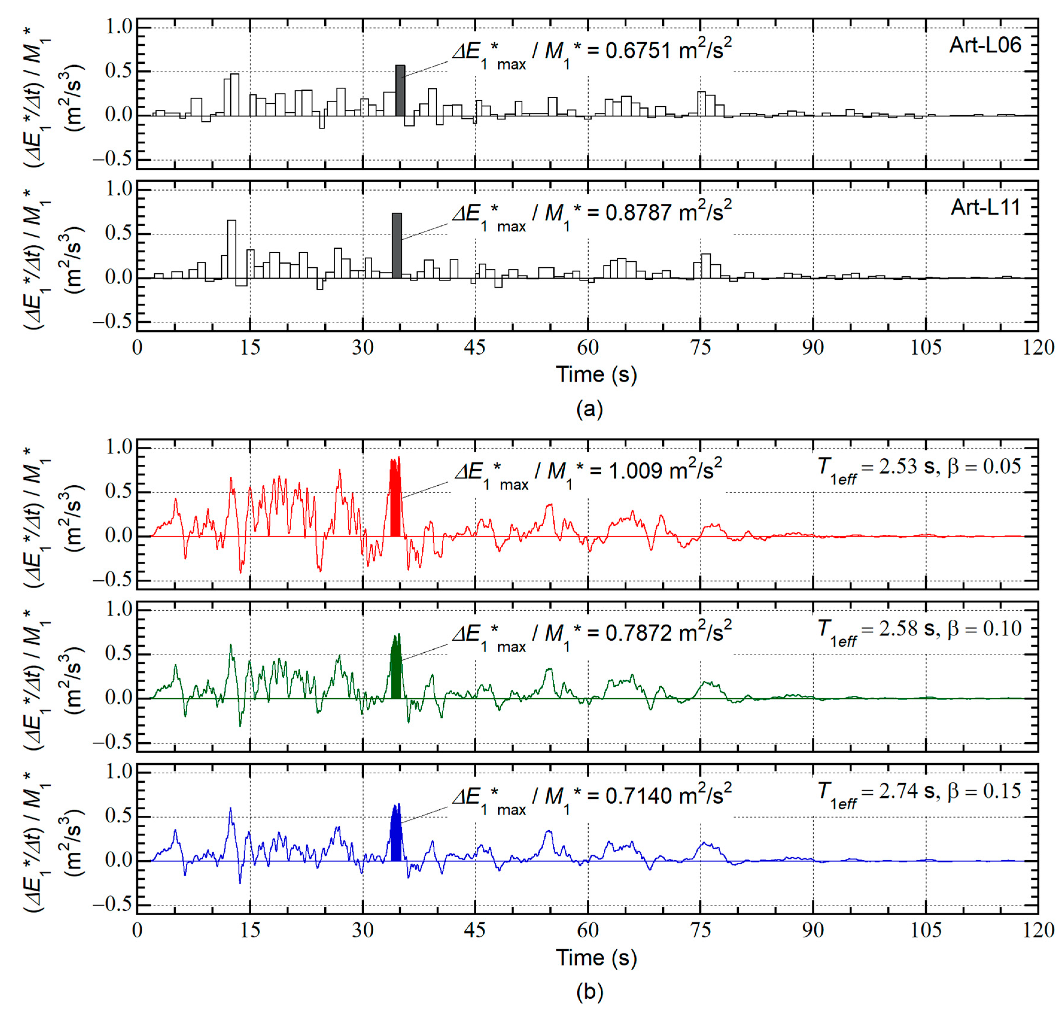
The time-history of the momentary input energy of the first modal response per unit mass (
) is compared with that calculated from the time-varying function in
Figure 17. In
Figure 17(a), the time-histories of the momentary input energy of the 16-story model (
= 0.05, Art-L-06 and Art-L-11) calculated from the nonlinear time-history analysis results are shown. In
Figure 17(b), the time-histories calculated from the time-varying function in Equation (27) are shown for each assumed complex damping ratio
: in the calculation of Equation (27), the natural period
is taken as the effective period of the first modal response corresponding to the predicted peak response point
.
The following observations can be made for
Figure 17.
This result implies that the accuracy of the maximum momentary input energy from the time-varying function strongly depends on the assumed complex damping ratio .
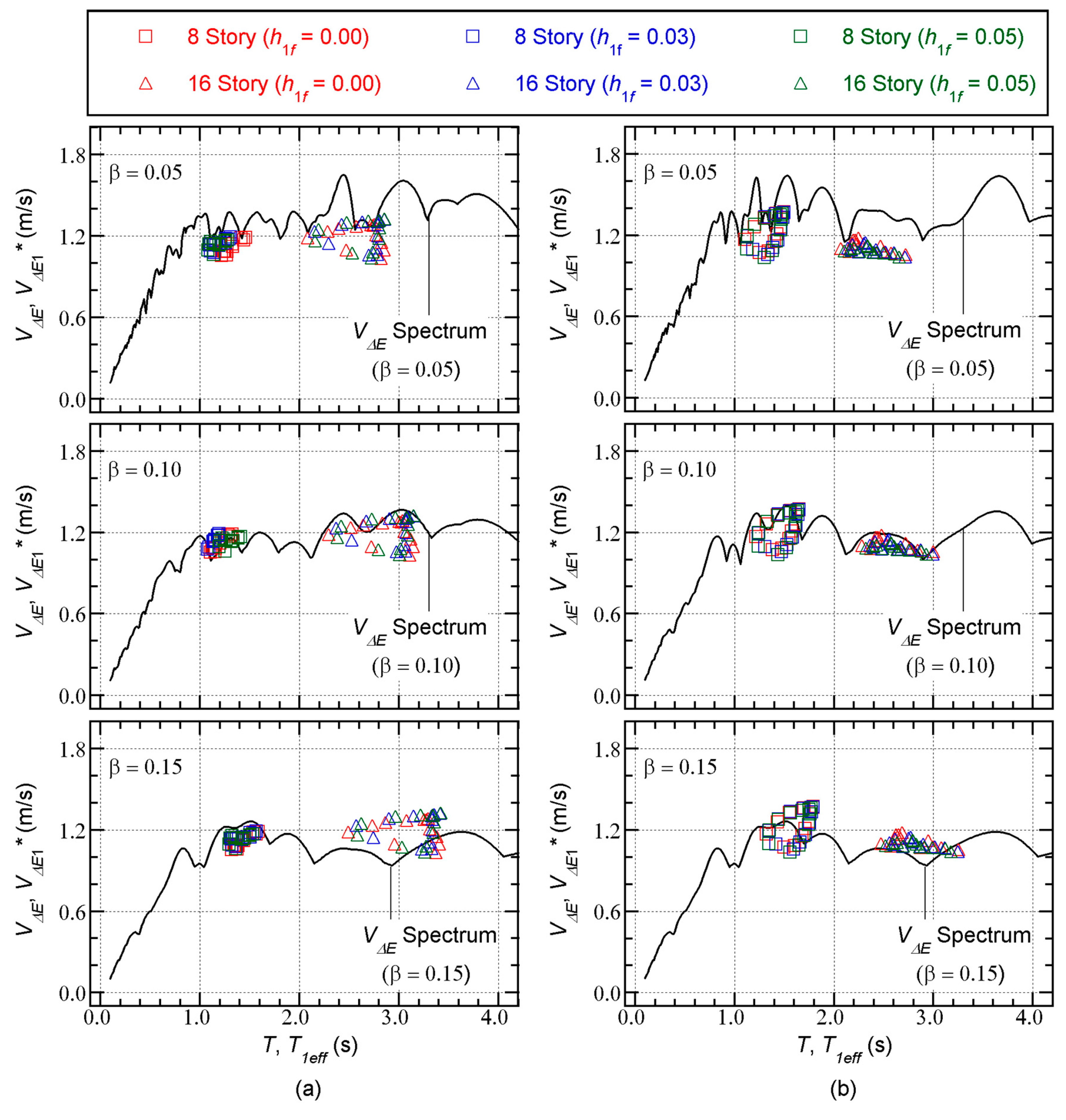
Figure 18 compares the
spectrum and the equivalent velocities of the maximum momentary input energy (
) obtained from the nonlinear time-history analysis results. In this figure, the effective period
is calculated from Equation (33). In addition, the
spectrum is calculated using the time-varying function as described in
Section 2.2.1.
The following observations can be made for
Figure 18.
In the case of
= 0.05 (shown at the top of
Figure 18), the nonlinear time-history analysis results are below the
spectrum.
In the case of
= 0.10 (shown in the middle of
Figure 18), the nonlinear time-history analysis results are in good agreement with the
spectrum.
In the case of
= 0.15 (shown at the bottom of
Figure 18), some of the nonlinear time-history analysis results are above the
spectrum.
The results shown in
Figure 18 imply that the most suitable value of
is 0.10 for the prediction of
using the
spectrum.
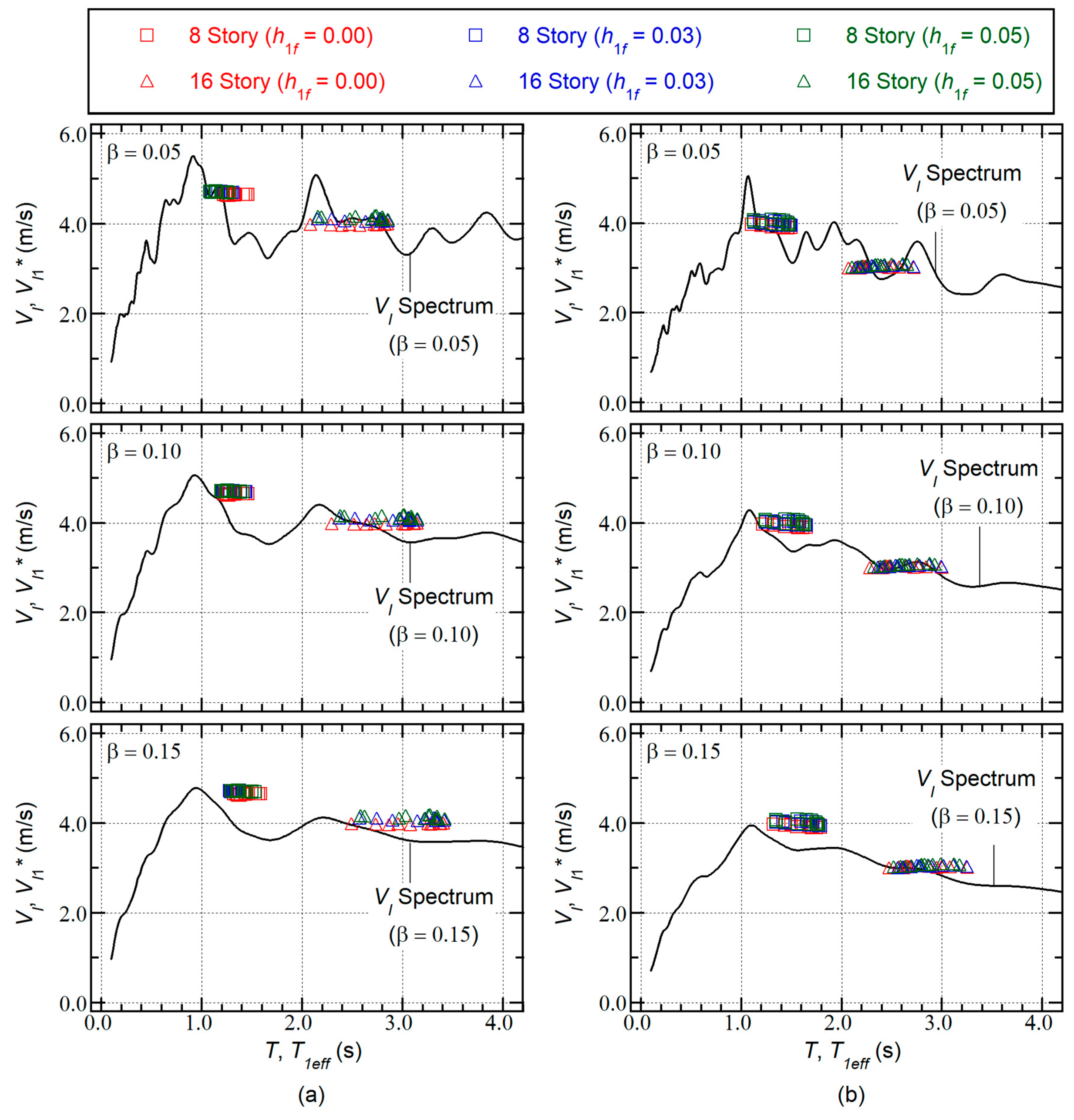
The
spectrum and the equivalent velocities of the cumulative input energy of the first modal response (
) obtained from the nonlinear time-history analysis results are compared in
Figure 19. The
spectrum shown in this figure is calculated using the time-varying function as described in
Section 2.2.1. This figure confirms that the most suitable value for
is 0.10.
Therefore, the equivalent velocities of the maximum momentary input energy and the cumulative energy ( and ) can be accurately predicted using the time-varying function, an appropriate effective period , and = 0.10. For the calculation of , Equation (33) is suitable.
5.2. Relationship between Maximum Momentary Input Energy of the First Modal Response and the Peak Equivalent Displacement
The relationship between the equivalent velocity of the maximum momentary input energy of the first modal response (
) and the peak equivalent displacement
is now examined by comparing the capacity curve (
–
relationship) described in
Section 2.1.
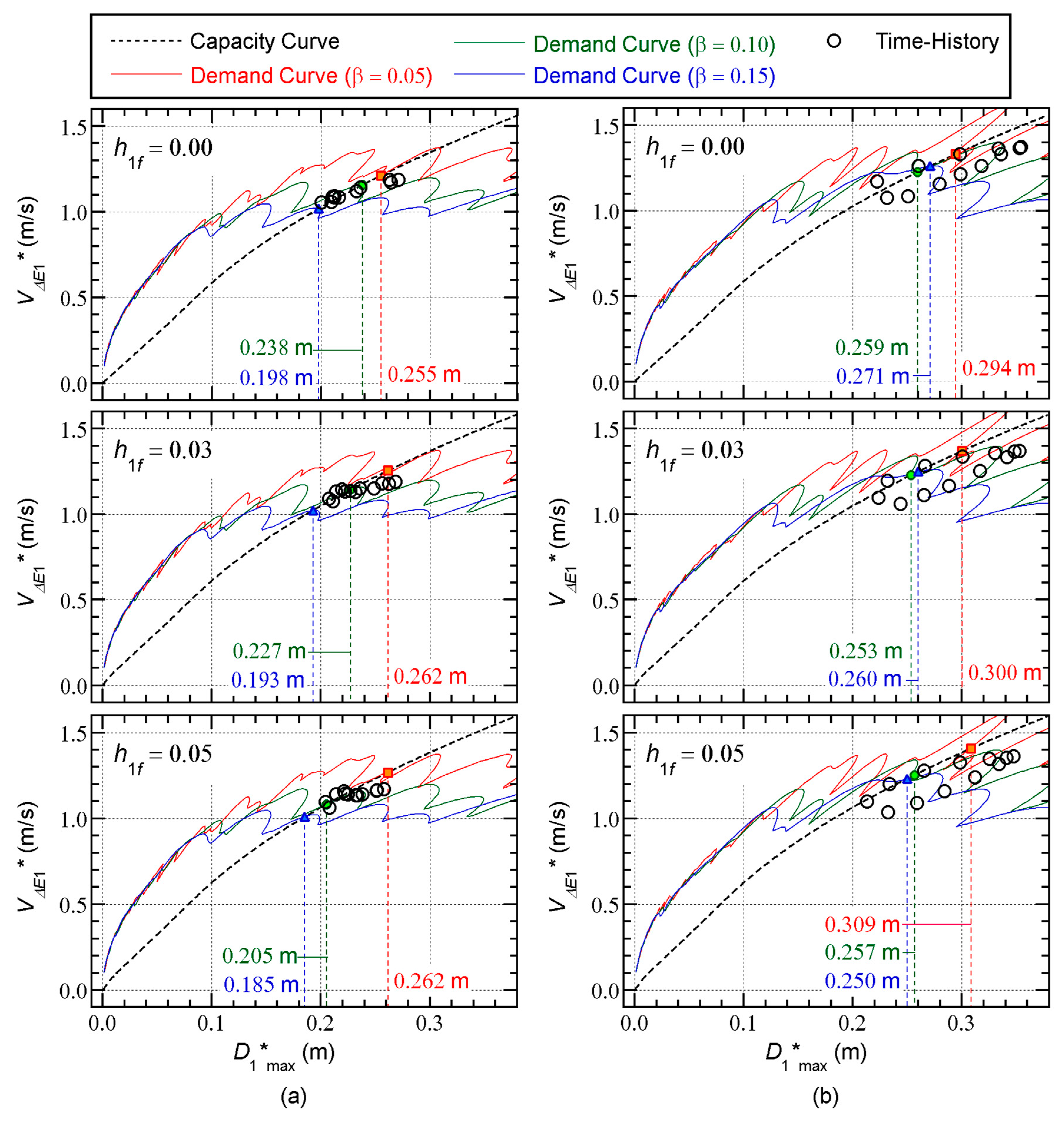
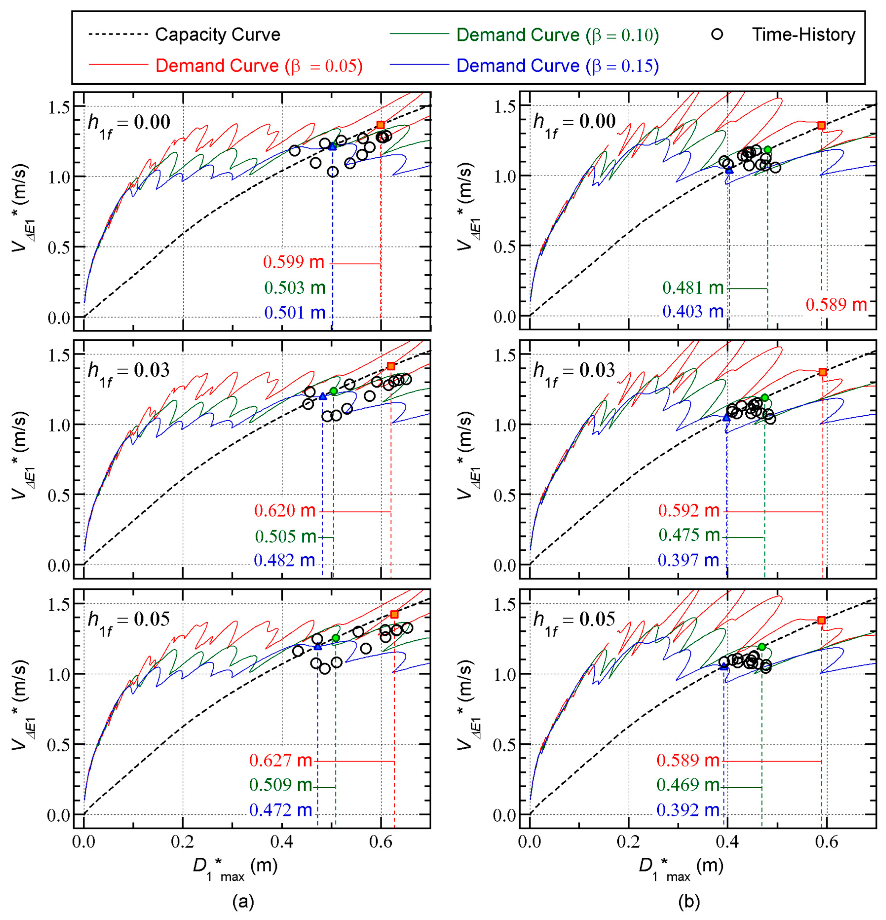
Figure 20 and
Figure 21 compare the capacity curve and the nonlinear time-history analysis results.
The following observations can be made for these figures.
Most of the nonlinear history analysis results are slightly below the capacity curve. The scatter of the nonlinear time-history analysis results is noticeable in the case of the Art-S series for the 8-story model and the Art-L series for the 16-story model.
In most cases, the predicted peak response point with = 0.05 gives the most conservative . The predicted with = 0.10 is slightly unconservative, and the predicted with = 0.15 is unconservative.
Therefore, for better predictions of the peak response, it is essential to calculate the capacity curve properly. Evaluating the dissipated energy during a half cycle of the structural response is very important, in addition to better predictions of the maximum momentary input energy.
5.3. Summary of Discussions
The above discussions can be summarized as follows.
The equivalent velocities of the maximum momentary input energy and the cumulative energy ( and ) can be properly predicted using the time-varying function, an appropriate effective period , and = 0.10. For the calculation of , Equation (33) is suitable.
For better predictions of the peak response, the capacity curve should be properly calculated. It is also very important to evaluate the dissipated energy during a half cycle of the structural response, in addition to better predictions of the maximum momentary input energy.
6. Conclusions
This article has proposed a nonlinear static procedure for predicting the seismic demand of regular RC ductile MRFs with steel damper columns. The main results and conclusions can be summarized as follows.
The time-varying function of the momentary energy input provides sufficiently accurate predictions of the maximum momentary input energy and the cumulative input energy of RC MRFs with steel damper columns. The time-history of the momentary input energy calculated using the time-varying function is close to the nonlinear time-history analysis results. An equation for calculating the effective period of the first modal response from the peak equivalent displacement and the equivalent velocity of the maximum momentary input energy has been developed. Based on the cases considered in this study, the recommended value of the complex damping ratio is 0.10.
The accuracy of the predicted local peak seismic demand (e.g., story drift, plastic rotation of the beam end, and shear strain of the damper panel) is acceptable, although some values are unconservative.
The accuracy of the predicted cumulative energy strain energy demand of the damper panel is acceptable, although some values are unconservative.
For better predictions of the peak response, the capacity curve must be properly calculated. It is also very important to evaluate the energy dissipated during a half cycle of the structural response, and to obtain better predictions of the maximum momentary input energy.
The main advantage of the proposed procedure is that both the peak and cumulative seismic demands of RC MRFs with steel damper columns can be predicted. In addition, as shown in previous studies [
28,
30], the time-varying function can be directly calculated from the Fourier amplitude and Fourier phase difference of ground motion. Therefore, the peak and cumulative seismic demands of RC MRFs with steel damper columns can be evaluated without knowing the time-history of ground motion. This means that researchers and analysts can eliminate otherwise unavoidable fluctuations from the nonlinear time-history analysis results. Note that the results and conclusions presented in this study are only valid for two RC MRFs with steel damper columns subjected to artificial ground motions. Therefore, apart from further verification using additional building models and ground motions, the following questions remain.
The above questions will be investigated in subsequent studies. However, they do not constitute a comprehensive list of all the issues requiring further research.
Author Contributions
Conceptualization, K.F. and M.S.; data curation, K.F. and M.S.; formal analysis, K.F. and M.S.; funding acquisition, K.F.; investigation, K.F. and M.S.; methodology, K.F.; project administration, K.F.; resources, K.F. and M.S.; software, K.F.; supervision, K.F.; validation, K.F.; visualization, K.F.; writing—original draft, K.F.; writing—review and editing, K.F. All authors have read and agreed to the published version of the manuscript.
Funding
This research received financial support from JFE Civil and Construction Corp.
Institutional Review Board Statement
Not applicable.
Informed Consent Statement
Not applicable.
Data Availability Statement
The data presented in this study are available on request from the corresponding author.
Acknowledgments
Valuable comments from Chizuru Irie and Mitsuhide Yoshinaga, JFE Civil Engineering, and Construction Corp. are appreciated. We thank Stuart Jenkinson, PhD, from Edanz (
https://jp.edanz.com/ac) for editing a draft of this manuscript.
Conflicts of Interest
The funders had no role in the design of the study; in the collection, analyses, or interpretation of data; in the writing of the manuscript; or in the decision to publish the results.
Appendix A. Formulation of the Dissipated Energy in a Half Cycle
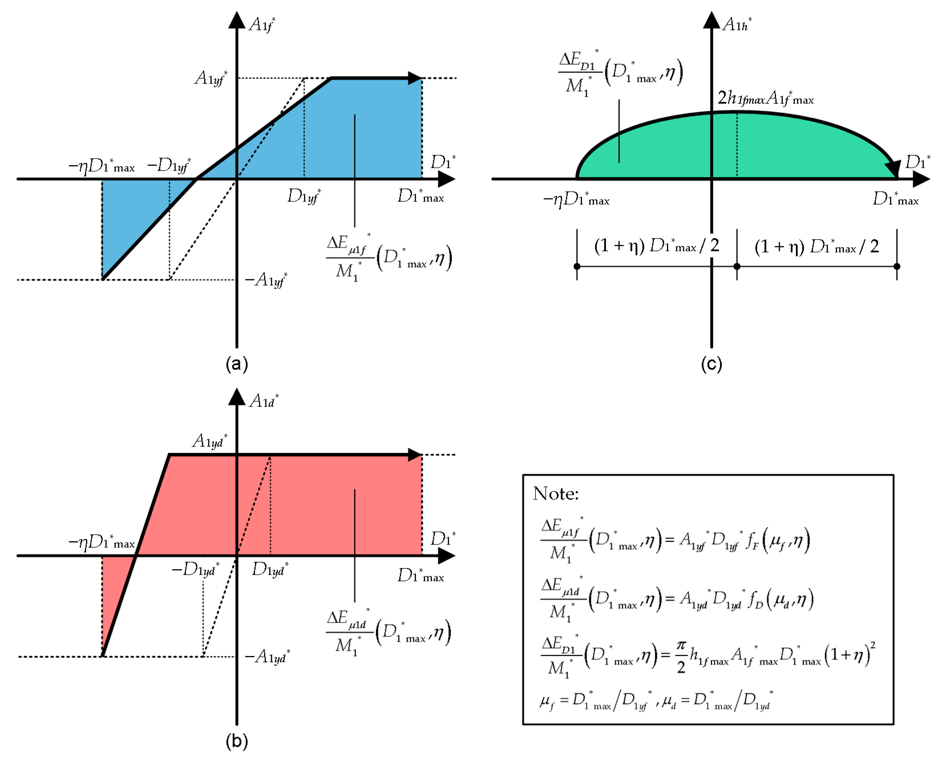
The dissipated energy in a half cycle of the equivalent SDOF model is formulated as follows.
Figure A1 shows simplified models for the calculation of the dissipated energy during a half cycle of the structural response. Here,
and
are the contributions of the hysteretic dissipated energies of RC MRFs and steel damper columns, respectively, while
is the contribution of viscous damping.
Figure A1.
Simplified models for calculation of the dissipated energy during a half cycle of the structural response: (a) contribution of RC MRFs; (b) contribution of steel damper columns; (c) contribution of viscous damping.
Figure A1.
Simplified models for calculation of the dissipated energy during a half cycle of the structural response: (a) contribution of RC MRFs; (b) contribution of steel damper columns; (c) contribution of viscous damping.
Considering the energy balance of the first modal response in a half cycle of the structural response, the maximum momentary input energy per unit mass (
) is calculated as
In Equation (A1),
is the ratio of displacements in the positive and negative directions. According to a previous study [
7],
and
are calculated as
In this study, the energy dissipation in a half cycle is simplified by calculating the average in the range
. The functions
and
are defined as
By substituting Equation (A5) into Equation (A7),
is calculated as
Similarly,
is calculated as
In addition, the average of the contribution from viscous damping is calculated as
Therefore, the maximum momentary input energy per unit mass (
) corresponding to the peak equivalent displacement (
) is calculated as
In the proposed procedure, the peak equivalent displacement (
) and the contribution of RC MRFs to the equivalent acceleration at the peak equivalent displacement (
) are replaced by the values obtained from pushover analysis at step
(
and
, respectively). In addition, the damping ratio at the peak equivalent displacement (
) is approximated as
In Equation (A13),
is the secant circular frequency of the first modal response at step
. Therefore, Equation (A12) can be rewritten as
Appendix B. Formulation of the Effective Period
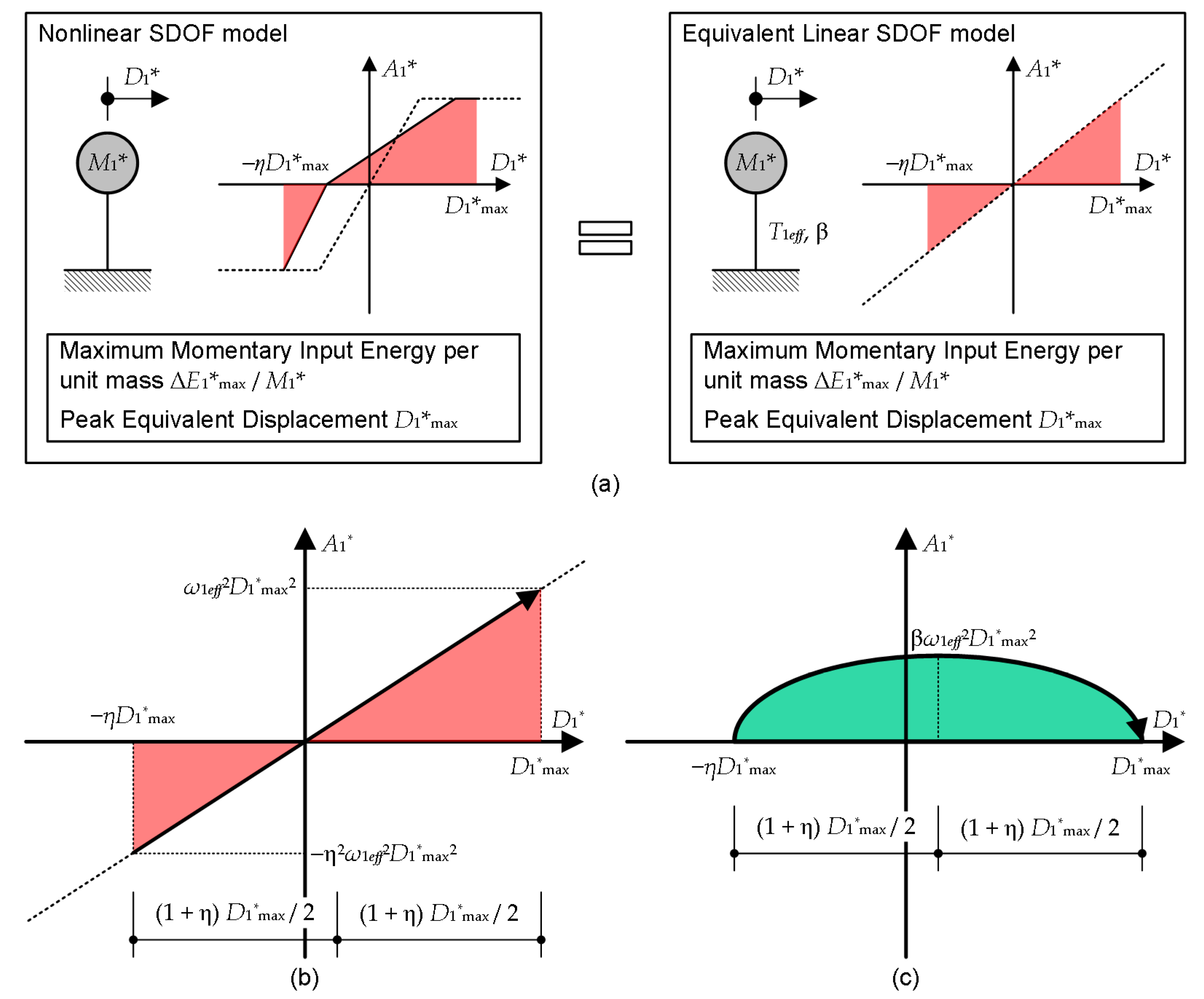
The effective period of the equivalent linear SDOF model is formulated as follows.
Figure A2 shows a scheme of the linearization of the equivalent SDOF model. As shown in
Figure A2(a), the nonlinear SDOF model is converted to the equivalent linear SDOF model.
Let us consider the case in which the peak equivalent displacement of the nonlinear SDOF model is
and the maximum momentary input energy per unit mass is
, as shown on the left of
Figure A2(a). The effective period and damping of the corresponding linear SDOF model are
and
, respectively. The peak equivalent displacement of the linear SDOF model is
when the maximum momentary input energy per unit mass is the same as in the nonlinear SDOF model (
), as shown on the left of
Figure A2(a).
The ratio of the displacements in the positive and negative directions (
) is assumed to be the same in both the nonlinear and equivalent linear SDOF models. From
Figure A2(b) and
Figure A2(c), the energy balance in a half cycle of the structural response can be expressed as
As discussed in
Appendix A, Equation (A16) can be simplified by calculating the average in the range
. On the right-hand side of Equation (A16),
Using Equation (A17), Equation (A16) can be simplified as
Therefore, the effective period
can be calculated from the equivalent velocity of the maximum momentary input energy of the equivalent SDOF model (
) and the peak equivalent displacement
as
Figure A2.
Scheme of the linearization of the equivalent SDOF model: (a) concept of the equivalent linearization; (b) contribution of the elastic strain energy; (c) contribution of the damping energy.
Figure A2.
Scheme of the linearization of the equivalent SDOF model: (a) concept of the equivalent linearization; (b) contribution of the elastic strain energy; (c) contribution of the damping energy.
Appendix C. Formulation of the Cumulative Dissipated Energy
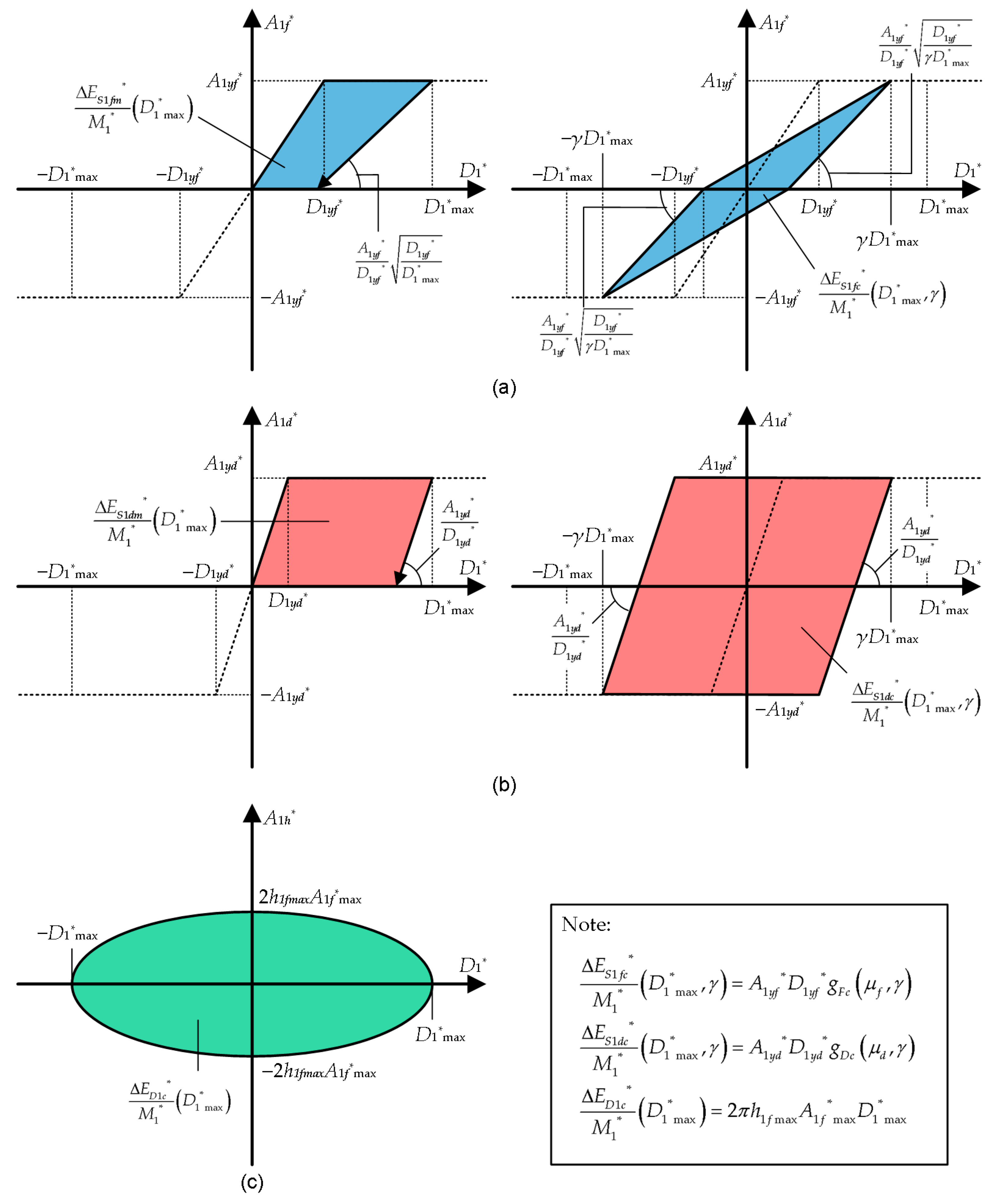
The cumulative dissipated energy of the equivalent SDOF model is formulated as follows.
Figure A3 shows simplified models for calculating the cumulative dissipated energy during a whole seismic event. Here,
and
are the hysteretic dissipated energy of RC MRFs per unit mass under monotonic and cyclic loading, respectively.
and
are the hysteretic dissipated energy of damper columns per unit mass under monotonic and cyclic loading, respectively.
is the damping dissipated energy per unit mass over a cycle of the structural response.
Figure A3.
Simplified models for calculation of the cumulative dissipated energy during a whole seismic event: (a) contribution of RC MRFs; (b) contribution of steel damper columns; (c) contribution of viscous damping.
Figure A3.
Simplified models for calculation of the cumulative dissipated energy during a whole seismic event: (a) contribution of RC MRFs; (b) contribution of steel damper columns; (c) contribution of viscous damping.
Given the peak equivalent displacement
, the dissipated strain energy of RC MRFs under monotonic loading per unit mass (
) can be calculated from the left of
Figure A3(a) as
Next, let us consider one loop of steady vibration (displacement amplitude:
, where
is the amplitude ratio), as shown on the right of
Figure A3(a). The function
is calculated as
In this study,
is simplified by calculating the average in the range
. The function
is defined as
Substituting Equation (A22) into Equation (A23),
is written as
Therefore, the dissipated strain energy of RC MRFs under cyclic loading per unit mass (
) can be calculated as
Similar to RC MRFs, the dissipated strain energy of the damper columns under monotonic and cyclic loading per unit mass (
and
) can be calculated from
Figure A3(b) as
From the right of
Figure A3(b),
is calculated as
By substituting Equation (A30) into Equation (A29),
is written as
Finally, the dissipated damping energy per unit mass over one cycle of the structural response (
) is calculated from
Figure A3(c) and Equation (A13) as
Appendix D. Model Properties
The properties of the members of the two models analyzed in this study are now described.
Table A1 presents the properties of sections at potential hinges of RC members in the 8-story model. Note that the cross-sections of all RC columns have dimensions of 800 mm × 800 mm, which are the same as those of the cross-section at the bottom of the first story. The cross-sections of the RC beams at the foundation level (Z
0) have dimensions of 800 mm × 2900 mm. The yield strength of the longitudinal reinforcement is assumed to be 1.1 × 390 = 429 N/mm
2. The assumed compressive strength of concrete is 45 N/mm
2 for the stories 1–4, and 36 N/mm
2 at and above the 5th story.
Table A2 presents the properties of selected damper columns in the 8-story model. The initial normal yield stress of the steel used for the damper panels is assumed to be 205 N/mm
2, whereas the normal yield stress after appreciable cyclic loading is assumed to be 300 N/mm
2.
Table A1.
Sections at potential hinges of RC members for 8-story model.
Table A1.
Sections at potential hinges of RC members for 8-story model.
| Member |
Location |
Width
(mm) |
Depth
(mm) |
Longitudinal Reinforcement |
| |
Z4 to Z8
|
500 |
900 |
5-D29 (Top and bottom) |
| Beam |
Z2 to Z3
|
500 |
900 |
5-D32 (Top and bottom) |
| |
Z1
|
550 |
900 |
5-D35 (Top and bottom) |
| Column |
1st Story (Bottom) |
800 |
800 |
16-D29 |
Table A2.
Steel damper columns for 8-story model.
Table A2.
Steel damper columns for 8-story model.
| Story |
Yield Strength |
Panel Thickness
(mm) |
Panel Height
(mm) |
Panel Sectional Area
(mm2) |
Column
(mm × mm × mm × mm) |
QyDL
(kN) |
QyDU
(kN) |
| 6 to 8 |
438 |
641 |
6 |
600 |
3700 |
H-600 × 200 × 12 × 25 |
| 4 to 5 |
626 |
916 |
9 |
600 |
5290 |
H-600 × 250 × 16 × 32 |
| 1 to 3 |
755 |
1105 |
9 |
700 |
6380 |
H-700 × 300 × 16 × 28 |
Table A3 presents the properties of sections at potential hinges of RC members in the 16-story model. Note that the cross-sections of all RC columns have dimensions of 900 mm × 900 mm, which are the same as those of the cross-section at the bottom of the first story. The cross-sections of the RC beams at the foundation level (Z
0) have dimensions of 800 mm × 2900 mm. The yield strength of the longitudinal reinforcement is assumed to be 429 N/mm
2. The assumed compressive strength of concrete is 60 N/mm
2 for stories 1–5, 54 N/mm
2 for stories 6–9, 45 N/mm
2 for stories 10–12, and 36 N/mm
2 at and above the 13th story.
Table A4 presents the properties of selected damper columns in the 16-story model. The properties of the steel used for the damper panel are the same as those for the 8-story model.
Table A3.
Sections at potential hinges of RC members for 16-story model.
Table A3.
Sections at potential hinges of RC members for 16-story model.
| Member |
Location |
Width
(mm) |
Depth
(mm) |
Longitudinal Reinforcement |
| |
Z7 to Z16
|
500 |
900 |
5-D29 (Top and bottom) |
| Beam |
Z2 to Z6
|
500 |
900 |
5-D32 (Top and bottom) |
| |
Z1
|
550 |
900 |
5-D35 (Top and bottom) |
| Column |
1st Story (Bottom) |
900 |
900 |
16-D35 |
Table A4.
Steel damper columns for 16-story model.
Table A4.
Steel damper columns for 16-story model.
| Story |
Yield Strength |
Panel Thickness
(mm) |
Panel Height
(mm) |
Panel Sectional Area
(mm2) |
Column
(mm × mm × mm × mm) |
QyDL
(kN) |
QyDU
(kN) |
| 11 to 16 |
438 |
641 |
6 |
600 |
3700 |
H-600 × 200 × 12 × 25 |
| 7 to 10 |
626 |
916 |
9 |
600 |
5290 |
H-600 × 250 × 16 × 32 |
| 1 to 6 |
755 |
1105 |
9 |
700 |
6380 |
H-700 × 300 × 16 × 28 |
References
- Wada, A.; Huang, Y.H.; Iwata, M. Passive damping technology for building in Japan. Prog. Struct. Eng. Mater. 2000, 8, 335–350. [CrossRef]
- Katayama, T.; Ito, S.; Kamura, H.; Ueki, T.; Okamoto, H. Experimental study on hysteretic damper with low yield strength steel under dynamic loading. In Proceedings of the 12th World Conference on Earthquake Engineering, Auckland, New Zealand, 30 January–4 February 2000.
- Fujii, K.; Miyagawa, K. Nonlinear seismic response of a seven-story steel reinforced concrete condominium retrofitted with low-yield-strength-steel damper columns. In Proceedings of the 16th European Conference on Earthquake Engineering, Thessaloniki, Greece, 18-21 June 2018.
- Fujii, K.; Sugiyama, H.; Miyagawa, K. Predicting the peak seismic response of a retrofitted nine-story steel reinforced concrete building with steel damper columns. WIT Transactions on the Built Environment. 2019, 185, 75-85. [CrossRef]
- Mukouyama, R.; Fujii, K.; Irie, C.; Tobari, R.; Yoshinaga, M.; Miyagawa, K. Displacement-controlled seismic design method of reinforced concrete frame with steel damper column. In Proceedings of the 17th World Conference on Earthquake Engineering, Sendai, Japan, 27 September–2 October 2021.
- Fujii, K.; Kato, M. Strength balance of steel damper columns and surrounding beams in reinforced concrete frames. WIT Transactions on the Built Environment. 2021, 202, 25-36. [CrossRef]
- Fujii, K. Peak and Cumulative Response of Reinforced Concrete Frames with Steel Damper Columns under Seismic Sequences. Buildings 2022, 12, 275. [CrossRef]
- Park, Y.J.; Ang, A.H.S. Mechanistic seismic damage model for reinforced concrete. J. Struct. Eng. ASCE 1985, 111, 722–739. [CrossRef]
- Architectural Institute of Japan (AIJ). Recommended Provisions for Seismic Damping Systems applied to Steel Structures, Architectural Institute of Japan: Tokyo, 2014. (In Japanese).
- Akiyama, H. Earthquake–Resistant Limit–State Design for Buildings; University of Tokyo Press: Tokyo, Japan, 1985.
- Uang, C.M.; Bertero, V.V. Evaluation of seismic energy in structures. Earthq. Eng. Struct. Dyn. 1990, 19, 77–90. [CrossRef]
- Fajfar, P.; Vidic, T. Consistent inelastic design spectra: Hysteretic and input energy. Earthq. Eng. Struct. Dyn. 1994, 23, 523–537. [CrossRef]
- Sucuoǧlu, H.; Nurtuǧ, A. Earthquake ground motion characteristics and seismic energy dissipation. Earthq. Eng. Struct. Dyn. 1995, 24, 1195–1213. [CrossRef]
- Nurtuǧ, A.; Sucuoǧlu, H. Prediction of seismic energy dissipation in SDOF systems. Earthq. Eng. Struct. Dyn. 1995, 24, 1215–1223. [CrossRef]
- Chai, Y.H.; Fajfar, P.; Romstad, K.M. Formulation of duration-dependent inelastic seismic design spectrum. J. Struct. Eng. 1998, 124, 913–921. [CrossRef]
- Cheng, Y.; Lucchini, A.; Mollaioli, F. Ground-motion prediction equations for constant-strength and constant-ductility input energy spectra. Bull. Earthq. Eng. 2020, 18, 37–55. [CrossRef]
- Fajfar, P.; Gaspersic, P. The N2 method for the seismic damage analysis of RC buildings. Earthq. Eng. Struct. Dyn. 1996, 25, 31–46. [CrossRef]
- Ghosh, S.; Datta, D.; Katakdhond A. A. Estimation of the Park–Ang damage index for planar multi-storey frames using equivalent single-degree systems. Engineering Structures, 2011, 33, 2509-2524. [CrossRef]
- Diaz, S.A.; Pujades, L.G.; Barbat, A.H.; Vargas, Y.F.; Hidalgo-Leiva D.A. Energy damage index based on capacity and response spectra. Engineering Structures, 2017, 152, 424-436. [CrossRef]
- Fajfar, P. Equivalent ductility factors, taking into account low-cycle fatigue. Earthq. Eng. Struct. Dyn. 1992, 21, 837–848. [CrossRef]
- D’Ambrisi, A.; Mezzi, M. An energy-based approach for nonlinear static analysis of structures. Bulletin of Earthquake Engineering, 2015, 13, 1513–1530. [CrossRef]
- Ucar, T. Computing input energy response of MDOF systems to actual ground motions based on modal contributions. Earthquakes and Structures, 2020, 18, 263-273.
- Yalçın, C.; Dindar, A.A.; Yüksel, E.; Özkaynak, H.; Büyüköztürk, O. Seismic design of RC frame structures based on energy-balance method. Engineering Structures, 2021, 237, 112220. [CrossRef]
- Benavent-Climent, A.; Mollaioli, F. (Eds.) Energy-Based Seismic Engineering; Springer Nature: Cham, Switzerland, 2021.
- Nakamura, T.; Hori, N.; Inoue, N. Evaluation of damaging properties of ground motions and estimation of maximum displacement based on momentary input energy. J. Struct. Constr. Eng. Trans. AIJ 1998, 63, 65–72. (In Japanese). [CrossRef]
- Inoue, N.; Wenliuhan, H.; Kanno, H.; Hori, N.; Ogawa, J. Shaking Table Tests of Reinforced Concrete Columns Subjected to Simulated Input Motions with Different Time Durations. In Proceedings of the 12th World Conference on Earthquake Engineering, Auckland, New Zealand, 30 January–4 February 2000.
- Hori, N.; Inoue, N. Damaging properties of ground motion and prediction of maximum response of structures based on momentary energy input. Earthq. Eng. Struct. Dyn. 2002, 31, 1657–1679. [CrossRef]
- Fujii, K.; Kanno, H.; Nishida, T. Formulation of the time-varying function of momentary energy input to a SDOF system by Fourier series. J. Jpn. Assoc. Earthq. Eng. 2019, 19, 247-266. [CrossRef]
- Fujii, K.; Murakami, Y. Bidirectional momentary energy input to a one-mass two-DOF system. In Proceedings of the 17th World Conference on Earthquake Engineering, Sendai, Japan, 20 September–2 November 2021.
- Fujii, K. Bidirectional seismic energy input to an isotropic nonlinear one-mass two-degree-of-freedom system. Buildings 2021, 11, 143. [CrossRef]
- Fujii, K.; Masuda, T. Application of Mode-Adaptive Bidirectional Pushover Analysis to an Irregular Reinforced Concrete Building Retrofitted via Base Isolation. Appl. Sci. 2021, 11, 9829. [CrossRef]
- Chopra, A.K.; Goel, R. K. A modal pushover analysis procedure for estimating seismic demands for buildings. Earthq. Eng. Struct. Dyn. 2002, 31, 561–582. [CrossRef]
- Antoniou, S.; Pinho, R. Advantages and limitation of adaptive and non-adaptive force-based pushover procedures, J. Earthq. Eng. 2004, 8, 497-522. [CrossRef]
- Antoniou, S.; Pinho, R. Development and verification of a displacement-based adaptive pushover procedure, J. Earthq. Eng. 2004, 8, 643-661. [CrossRef]
- Jan, T. S.; Ming Liu, M. W.; Kao, Y. C. An upper-bound pushover analysis procedure for estimating the seismic demands of high-rise buildings. Eng. Struct. 2004, 26, 117-128. [CrossRef]
- Sucuoǧlu, H.; Günay M. S. Generalized force vectors for multi-mode pushover analysis. Earthq. Eng. Struct. Dyn. 2011, 40, 55–74. [CrossRef]
- Brozovič, M., Dolšek, M. Envelope-based pushover analysis procedure for the approximate seismic response analysis of buildings. Earthq. Eng. Struct. Dyn. 2014, 43, 77–96. [CrossRef]
- Surmeli, M.; Yuksel, E. A variant of modal pushover analyses (VMPA) based on a non-incremental procedure. Bull. Earthquake Eng. 2015, 13, 3353–3379. [CrossRef]
- Rahmani, A. Y.; Bourahla, N.; Bento, R.; Badaoui, M. An improved upper-bound pushover procedure for seismic assessment of high-rise moment resisting steel frames. Bull. Earthquake Eng. 2018, 16, 315–339. [CrossRef]
- Baber, T.T.; and Noori, M.M. Random vibration of degrading, pinching systems. J. Eng. Mech. ASCE 1985, 111, 1010–1026. [CrossRef]
- Elwood, K. J.; Sarrafzadeh, M.; Pujol, S.; Liel, A.; Murray, P.; Shah, P.; Brooke, N. J. Impact of prior shaking on earthquake response and repair requirements for structures – studies from ATC-145. In Proceedings of the NZSEE 2021 Annual Conference, Christchurch, 14-16 April 2021.
- Building Center of Japan (BCJ). The Building Standard Law of Japan on CD-ROM; The Building Center of Japan: Tokyo, Japan, 2016.
- Fujii, K. Prediction of the largest peak nonlinear seismic response of asymmetric buildings under bi-directional excitation using pushover analyses. Bull. Earthq. Eng. 2014, 12, 909-938. [CrossRef]
Figure 1.
Outline of the proposed procedure.
Figure 1.
Outline of the proposed procedure.
Figure 2.
Schemes for the prediction of the peak and cumulative responses of the equivalent SDOF model: (a) capacity curve; (b) demand curve; (c) prediction of the peak equivalent displacement; (d) prediction of the cumulative input energy.
Figure 2.
Schemes for the prediction of the peak and cumulative responses of the equivalent SDOF model: (a) capacity curve; (b) demand curve; (c) prediction of the peak equivalent displacement; (d) prediction of the cumulative input energy.
Figure 3.
RC MRF building models with damper columns: (a) structural plan; (b) structural elevation of 8-story model; (c) structural elevation of 16-story model.
Figure 3.
RC MRF building models with damper columns: (a) structural plan; (b) structural elevation of 8-story model; (c) structural elevation of 16-story model.
Figure 4.
Time histories of the artificial ground acceleration: (a) Art-L-00; (b) Art-S-00.
Figure 4.
Time histories of the artificial ground acceleration: (a) Art-L-00; (b) Art-S-00.
Figure 5.
Pseudo-acceleration spectra of the artificial ground acceleration: (a) Art-L series; (b) Art-S series.
Figure 5.
Pseudo-acceleration spectra of the artificial ground acceleration: (a) Art-L series; (b) Art-S series.
Figure 6.
Capacity curves of building models: (a) 8-story model; (b) 16-story model.
Figure 6.
Capacity curves of building models: (a) 8-story model; (b) 16-story model.
Figure 7.
Demand curve of input ground motions: (a) Art-L series; (b) Art-S series.
Figure 7.
Demand curve of input ground motions: (a) Art-L series; (b) Art-S series.
Figure 8.
Prediction of the peak response point ( = 0.05): (a) 8-story model (Art-L series); (b) 16-story model (Art-L series); (c) 8-story model (Art-S series); (d) 16-story model (Art-S series).
Figure 8.
Prediction of the peak response point ( = 0.05): (a) 8-story model (Art-L series); (b) 16-story model (Art-L series); (c) 8-story model (Art-S series); (d) 16-story model (Art-S series).
Figure 9.
Prediction of the equivalent velocity of the cumulative input energy for the first modal response ( = 0.05): (a) 8-story model (Art-L series); (b) 16-story model (Art-L series); (c) 8-story model (Art-S series); (d) 16-story model (Art-S series).
Figure 9.
Prediction of the equivalent velocity of the cumulative input energy for the first modal response ( = 0.05): (a) 8-story model (Art-L series); (b) 16-story model (Art-L series); (c) 8-story model (Art-S series); (d) 16-story model (Art-S series).
Figure 10.
Prediction of the energy demand of the overall building (8-story model): (a) Art-L series; (b) Art-S series.
Figure 10.
Prediction of the energy demand of the overall building (8-story model): (a) Art-L series; (b) Art-S series.
Figure 11.
Prediction of the energy demand of the overall building (16-story model): (a) Art-L series; (b) Art-S series.
Figure 11.
Prediction of the energy demand of the overall building (16-story model): (a) Art-L series; (b) Art-S series.
Figure 12.
Comparisons of the peak story drift: (a) 8-story model ( = 0.00); (b) 16-story model ( = 0.00); (c) 8-story model ( = 0.03); (d) 16-story model ( = 0.03); (e) 8-story model ( = 0.05); (f) 16-story model ( = 0.05).
Figure 12.
Comparisons of the peak story drift: (a) 8-story model ( = 0.00); (b) 16-story model ( = 0.00); (c) 8-story model ( = 0.03); (d) 16-story model ( = 0.03); (e) 8-story model ( = 0.05); (f) 16-story model ( = 0.05).
Figure 13.
Comparisons of the peak plastic hinge rotation of the beam: (a) 8-story model ( = 0.00); (b) 16-story model ( = 0.00); (c) 8-story model ( = 0.03); (d) 16-story model ( = 0.03); (e) 8-story model ( = 0.05); (f) 16-story model ( = 0.05).
Figure 13.
Comparisons of the peak plastic hinge rotation of the beam: (a) 8-story model ( = 0.00); (b) 16-story model ( = 0.00); (c) 8-story model ( = 0.03); (d) 16-story model ( = 0.03); (e) 8-story model ( = 0.05); (f) 16-story model ( = 0.05).
Figure 14.
Comparisons of the peak shear strain of the damper panels: (a) 8-story model ( = 0.00); (b) 16-story model ( = 0.00); (c) 8-story model ( = 0.03); (d) 16-story model ( = 0.03); (e) 8-story model ( = 0.05); (f) 16-story model ( = 0.05).
Figure 14.
Comparisons of the peak shear strain of the damper panels: (a) 8-story model ( = 0.00); (b) 16-story model ( = 0.00); (c) 8-story model ( = 0.03); (d) 16-story model ( = 0.03); (e) 8-story model ( = 0.05); (f) 16-story model ( = 0.05).
Figure 15.
Comparisons of the normalized cumulative strain energy of the damper panels: (a) 8-story model ( = 0.00); (b) 16-story model ( = 0.00); (c) 8-story model ( = 0.03); (d) 16-story model ( = 0.03); (e) 8-story model ( = 0.05); (f) 16-story model ( = 0.05).
Figure 15.
Comparisons of the normalized cumulative strain energy of the damper panels: (a) 8-story model ( = 0.00); (b) 16-story model ( = 0.00); (c) 8-story model ( = 0.03); (d) 16-story model ( = 0.03); (e) 8-story model ( = 0.05); (f) 16-story model ( = 0.05).
Figure 16.
Time-history and hysteresis of the first modal response (16-story model, = 0.05, Art-L): (a) time-history of ground acceleration; (b) time-history of equivalent displacement of the first modal response; (c) hysteresis of the first modal response.
Figure 16.
Time-history and hysteresis of the first modal response (16-story model, = 0.05, Art-L): (a) time-history of ground acceleration; (b) time-history of equivalent displacement of the first modal response; (c) hysteresis of the first modal response.
Figure 17.
Comparisons of the time-history of the momentary energy input of the first modal response (16-story model, Art-L): (a) momentary energy input obtained from the time-history analysis; (b) momentary energy input calculated using time-varying function.
Figure 17.
Comparisons of the time-history of the momentary energy input of the first modal response (16-story model, Art-L): (a) momentary energy input obtained from the time-history analysis; (b) momentary energy input calculated using time-varying function.
Figure 18.
Comparisons of the spectrum and obtained from the time-history analysis: (a) Art-L series; (b) Art-S series.
Figure 18.
Comparisons of the spectrum and obtained from the time-history analysis: (a) Art-L series; (b) Art-S series.
Figure 19.
Comparisons of the spectrum and obtained from the time-history analysis: (a) Art-L series; (b) Art-S series.
Figure 19.
Comparisons of the spectrum and obtained from the time-history analysis: (a) Art-L series; (b) Art-S series.
Figure 20.
Comparisons between the capacity curve and the − relationship obtained from the time-history analysis results (8-story model): (a) Art-L series; (b) Art-S series.
Figure 20.
Comparisons between the capacity curve and the − relationship obtained from the time-history analysis results (8-story model): (a) Art-L series; (b) Art-S series.
Figure 21.
Comparisons between the capacity curve and the − relationship obtained from the time-history analysis results (16-story model): (a) Art-L series; (b) Art-S series.
Figure 21.
Comparisons between the capacity curve and the − relationship obtained from the time-history analysis results (16-story model): (a) Art-L series; (b) Art-S series.
Table 1.
Natural period of the models at the initial stage.
Table 1.
Natural period of the models at the initial stage.
| |
8-story model |
16-story model |
|
(s) |
0.5611 |
1.1163 |
|
(s) |
0.1869 |
0.3693 |
|
(s) |
0.1053 |
0.2062 |
|
Disclaimer/Publisher’s Note: The statements, opinions and data contained in all publications are solely those of the individual author(s) and contributor(s) and not of MDPI and/or the editor(s). MDPI and/or the editor(s) disclaim responsibility for any injury to people or property resulting from any ideas, methods, instructions or products referred to in the content. |
© 2023 by the authors. Licensee MDPI, Basel, Switzerland. This article is an open access article distributed under the terms and conditions of the Creative Commons Attribution (CC BY) license (http://creativecommons.org/licenses/by/4.0/).
