Application of RRAP Reliability Optimization as Test of Nature Inspired Algorithms

Preprint

Article

Application of RRAP Reliability Optimization as Test of Nature Inspired Algorithms

Altmetrics

Downloads

122

Views

Comments

A peer-reviewed article of this preprint also exists.

Adam Pieprzycki^*,Bogusław Filipowicz

This version is not peer-reviewed

Submitted:

04 January 2023

Posted:

06 January 2023

You are already at the latest version

Alerts

Abstract

This paper considers the application of two selected algorithms (Cuckoo Search CS, Firefly Algorithm FA) to determine and maximize the reliability of a two complex system known from the literature. This system operates with resource constraints. In addition, several classical methods for determining the reliability of systems have been applied. Although the CS algorithm is known for its effectiveness as it uses the Lévy flight, for the presented optimization tasks the FA firefly algorithm in the considered parameter range proved to be more effective. The presented results broaden the existing discussion on the application of nature-inspired algorithms for solving RRAP (Reliability Redundancy Allocation Problem) problems. From this point of view, two described test scenarios can be considered as a suitable tool for validating other algorithms in RRAP problems. Not only the values of the criterion functions can be compared, but also other introduced parameters and statistical analyse of variance (ANOVA) with post-hoc RIR Tuckey test was discussed.

Keywords:

Subject: Engineering - Electrical and Electronic Engineering

1. Introduction

The reliability of a non–renewable object can be defined as the ability to retain such properties that allow it to be used for its intended purpose [1] The optimization of the considered topic may concern increasing reliability (increasing safety) or decreasing it in order to reduce costs. Increasing reliability may concern each component of the system or involve the introduction of redundancy (redundancy) in individual subsystems. For a extremely reliable system, it is necessary to design the system with redundant elements in a balance between: price, weight, volume or lifetime. This type of non–linear design with (resource) constraints is called RRAP (Reliability Redundancy Allocation Problem). The problem of reliability optimization considering redundancy can be qualified as a non–linear programming problem with one or more constraints. The solution of the optimization task consists in the optimal allocation of system components (number of elements, reliability level), maximizing the total reliability while satisfying the existing constraints. RRAP belongs to NP–hard problems. Such redundancy is desirable and provides protection in the event that part of the system fails. A critical component may be duplicated or several components (even three or more) used in parallel to avoid system breakdown. In engineering, this can be the parallel operation of several components (e.g., temperature sensor contacts, etc.), or redundant devices in the power grid. A classic example of increasing system reliability in computing is the use of RAID (Redundant Array of Independent Disks) disk arrays. The objective of reliability optimization is to select (calculate) the number of redundant components and their reliability values in each subsystem, and to maximize the total system reliability. The criterion functions presented in the following part of the article describe the reliability of the system (system), which has been taken as a quality indicator (criterion function) and is subject to maximization with the introduced constraints. In an attempt to solve the discussed reliability optimization problems of complex systems, the results obtained using two selected heuristic algorithms were considered and compared. These are algorithms based on the social behavior of animals, birds or insects. Two selected optimization algorithms have been applied: Firefly Algorithm FA [2] and Cuckoo Search CS [3]. In the analyzed class of problems, the FA firefly algorithm is known for its effectiveness. The use of another algorithm (CS cuckoo search algorithm) allowed us to compare their accuracy in solving two optimization problems [4,5,6]. Recent studies show that CS is potentially far more efficient than PSO (Particle Swarm Optimisation), genetic algorithms, and other algorithms [2]. In the meanwhile, scientists, especially theorists, ask the question of why animals do Lévy flight, which fascinates researchers from various disciplines from ecology to physics [7]. Application of artificial intelligence in reliability optimization of systems successfully previously applied also in power grid optimization (k-terminal grid model) using swarm optimization algorithms [8]. In that work, a reliability function in the form of BDD (Binary Decision Diagram) diagrams and a combined decomposition EED (Edge Expansion Diagrams) [9], CAE (Composition After Expansion) [10] and fixed-sink algorithm for k-terminal networks [11].

2. Problem Definition

The issue under discussion concerns the maximization of the criterion function:

m a x (F_{c} (r, n)),

(1)

within constraints:

g_{y} (r, n) \leq b_{y},

(2)

0 \leq r \leq 1, n \in Z^{+}, 1 \leq y \leq k, y \in Z^{+}, k \in Z^{+},

(3)

where:

F_{c} (r, n)

– system reliability function,

n

– vector of the number of elements in the various subsystems,

r

– the reliability vector of each element in each subsystem,

g_{y}

– the physical characteristics of the element in subsystem for constraint number y,

b_{y}

– upper limit for constraint number y, k– number of constraints.

3. Models of the RRAP System

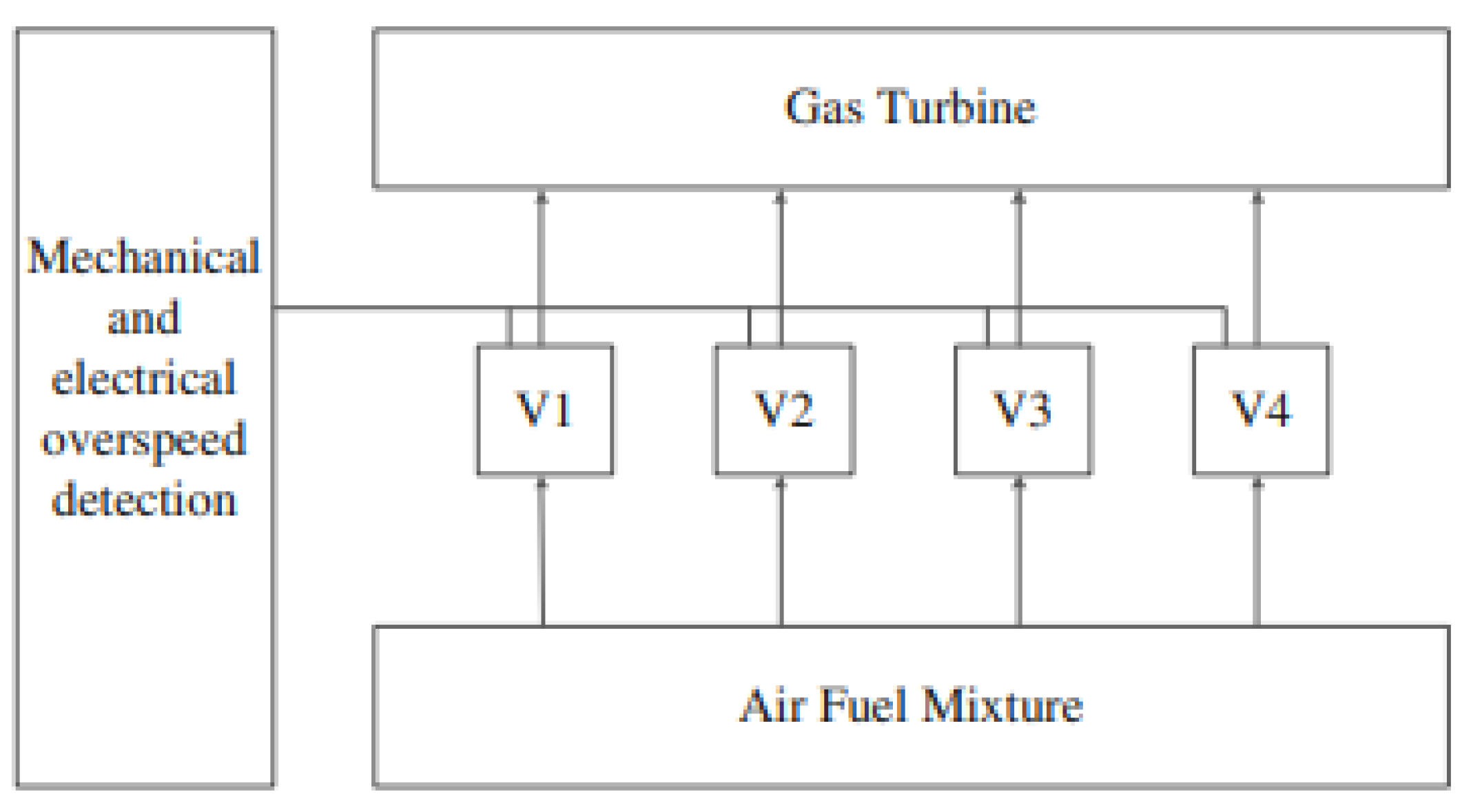
The criterion functions for the scenarios considered have been derived in detail in the literature [3,4,12]. Another—not discussed in the article—test cases are: an overspeed system for a gas turbine (Figure 1) or a more complicated 15-unit system reliability problem with different combinations of parameters [12].

3.1. Scenario 1—Bridge System

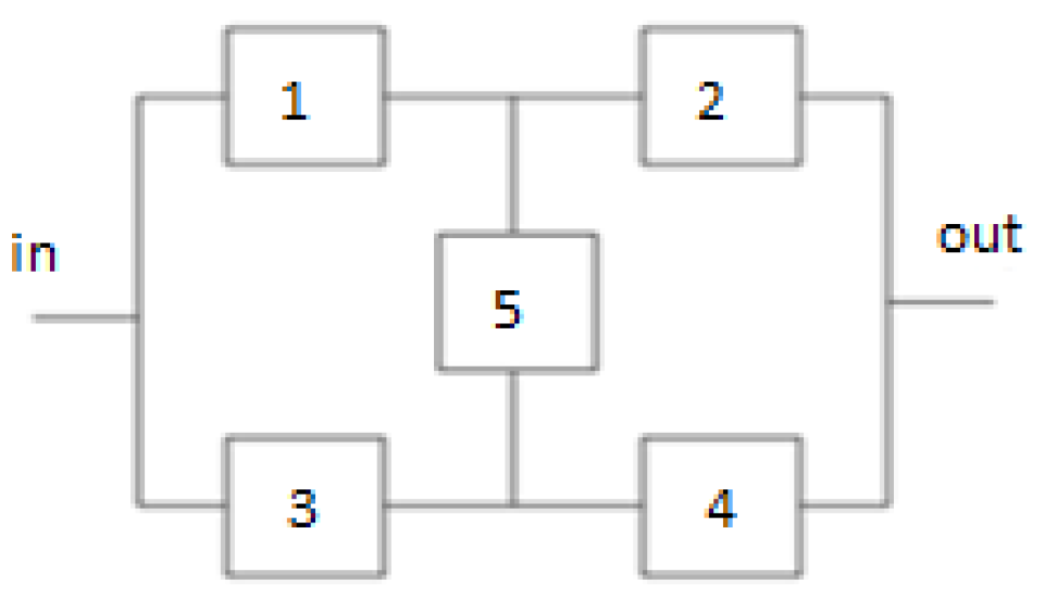
In the first scenario, the five–element bridge system (Figure 2) [3,4,12] was considered.

The criterion function of a bridge system has been derived in detail in literature can be formulated as:

\begin{matrix} F_{c_{1}} (r, n) = R_{1} \cdot R_{2} + R_{3} \cdot R_{4} + R_{1} \cdot R_{4} \cdot R_{5} + R_{2} \cdot R_{3} \cdot R_{5} - R_{1} \cdot R_{2} \cdot R_{3} \cdot R_{4} - R_{1} \cdot R_{2} \cdot R_{3} \cdot R_{5} + \\ - R_{1} \cdot R_{2} \cdot R_{4} \cdot R_{5} - R_{1} \cdot R_{3} \cdot R_{4} \cdot R_{5} - R_{2} \cdot R_{3} \cdot R_{4} \cdot R_{5} + 2 \cdot R_{1} \cdot R_{2} \cdot R_{3} \cdot R_{4} \cdot R_{5}, \end{matrix}

(4)

where the individual reliability values

R_{i}

of each subsystem are calculated as:

R_{i} = 1 - {(1 - r_{i})}^{n_{i}}, \forall i \in {1, 2, \dots, m_{1}} .

(5)

For a bridged system occurs the optimization of 10 decision variables (five variables

r_{i}

and another five variables

n_{i}

with integer values). Three constraints (

k_{1}

=3) scenario 1 of total weight and volume (V), cost (C), lifetime (T) and system weight (W) were introduced (Table 1):

g_{1} (r, n) = \sum_{i = 1}^{m_{1}} w_{i} \cdot v_{i}^{2} \cdot n_{i}^{2} - V \leq 0,

(6)

g_{2} (r, n) = \sum_{i = 1}^{m_{1}} α_{i} \cdot {(- \frac{T}{l n (r_{i})})}^{β} \cdot (n_{i} + e^{0.25 \cdot n_{i}}) - C \leq 0,

(7)

g_{3} (r, n) = \sum_{i = 1}^{m_{1}} w_{i} \cdot n_{i} \cdot e^{0.25 \cdot n_{i}} - W \leq 0,

(8)

0 \leq i \leq m_{1}, 0 \leq r_{i} \leq 1, n_{i} \in Z^{+},

(9)

where:

m_{1}

– number of subsystems in the whole system (

m_{1}

=5) at scenario 1,

n_{i}

– number of elements in i–th subsystem,

r_{i}

– the reliability of each element in i–th subsystem,

R_{i}

– reliability of i–th subsystem,

α_{i}

β_{i}

– physical characteristics of element in i–th subsystem,

w_{i}

v_{i}

c_{i}

– weight, volume and cost of the element in i–th subsystem.

In order to compare the results obtained with other solutions found in the literature, the parameter settings of the bridge system were adopted as shown in Table 2 [4]. Other methods of system reliability analysis are also used, such as optimization using the path method, for which the objective function takes the form:

\begin{matrix} F_{c_{2}} (r, n) = 1 - (1 - R_{1} \cdot R_{2}) \cdot (1 - R_{3} \cdot R_{4}) \cdot (1 - R_{1} \cdot R_{4} \cdot R_{5}) \cdot (1 - R_{2} \cdot R_{3} \cdot R_{5}), \end{matrix}

(10)

or a cutting method for which the criterion function can be expressed as:

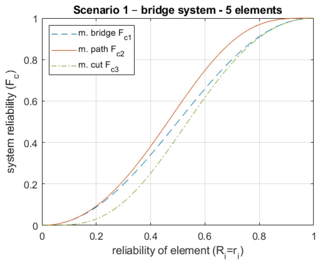
\begin{matrix} F_{c_{3}} (r, n) = (1 - (1 - R_{1}) \cdot (1 - R_{3})) \cdot (1 - (1 - R_{2}) \cdot (1 - R_{4})) \cdot (1 - (1 - R_{2} \cdot (1 - R_{3}) \cdot (1 - R_{5})) \cdot \\ \cdot (1 - (1 - R_{1}) \cdot (1 - R_{4}) \cdot (1 - R_{5})) . \end{matrix}

(11)

The reliability of the system calculated with the method of minimum cuts is always smaller (11) (it is the lower limit) than the value of reliability calculated with the method of minimal path

F_{c_{2}}

(10)—it is the upper limit. This difference can be a space for exact optimization (Figure 3).

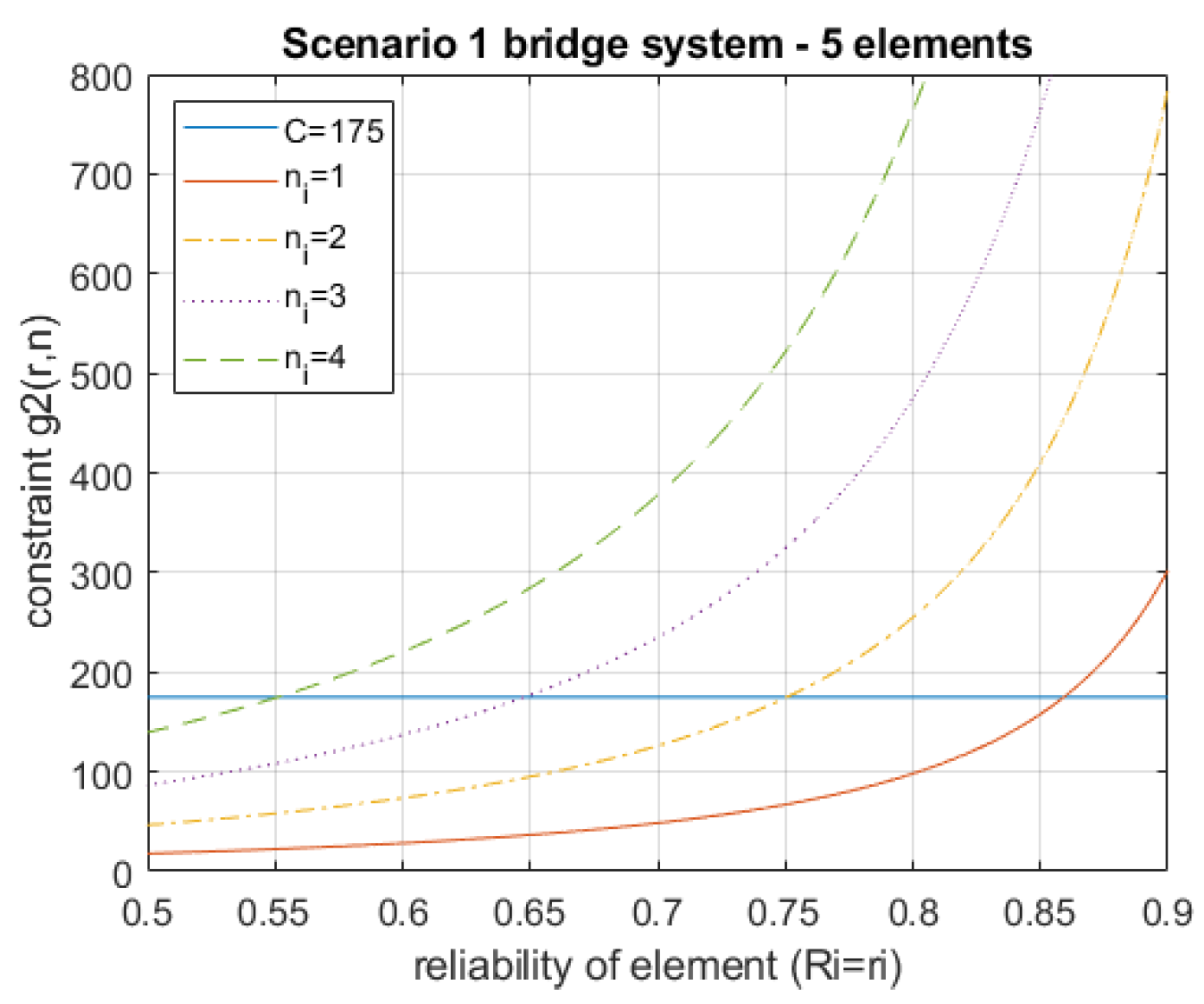
Analyzing the constraints adopted for the analyzed model, it can be noted that the second constraint (

g_{2}

(r,n)) (7) significantly affects the permissible values of element reliability (Figure 4).

3.2. Scenario 2—System Consisting 10 Elements

The criterion function of a ten elements system (Figure 5) is more complicated than bridge system [4,12] and can be formulated as:

\begin{matrix} F_{c_{4}} (r, n) = R_{1} \cdot R_{2} \cdot R_{3} \cdot R_{4} + (R_{1} \cdot R_{2} \cdot R_{6} \cdot R_{10}) \cdot (Q_{3} + R_{3} \cdot Q_{4}) + (R_{1} \cdot R_{5} \cdot R_{9} \cdot R_{10}) \cdot (Q_{2} + \\ + R_{2} \cdot Q_{3} \cdot Q_{6} + R_{2} \cdot R_{3} \cdot Q_{4} \cdot Q_{6}) + R_{7} \cdot R_{8} \cdot R_{9} \cdot R_{10} \cdot (Q_{1} + R_{1} \cdot R_{2} \cdot Q_{3} \cdot Q_{5} \cdot Q_{6} + \\ + R_{1} \cdot R_{3} \cdot Q_{4} \cdot Q_{5} \cdot Q_{6}) + R_{2} \cdot R_{3} \cdot R_{4} \cdot R_{5} \cdot R_{7} \cdot R_{8} \cdot Q_{1} \cdot (Q_{9} + R_{9} \cdot Q_{10}) + \\ + Q_{1} \cdot R_{3} \cdot R_{4} \cdot R_{6} \cdot R_{7} \cdot R_{8} \cdot Q_{10} \cdot (Q_{2} + R_{2} \cdot Q_{5}) + \\ + Q_{1} \cdot Q_{2} \cdot R_{3} \cdot R_{4} \cdot R_{6} \cdot R_{7} \cdot R_{8} \cdot R_{9} \cdot Q_{10} + R_{1} \cdot Q_{2} \cdot R_{3} \cdot R_{4} \cdot R_{5} \cdot R_{6} \cdot R_{9} \cdot Q_{10} \cdot (Q_{7} + R_{7} \cdot Q_{8}) + \\ + Q_{1} \cdot R_{2} \cdot R_{5} \cdot R_{6} \cdot R_{7} \cdot R_{8} \cdot Q_{9} \cdot R_{10} \cdot (Q_{3} + R_{3} \cdot Q_{4}), \end{matrix}

(12)

where:

R_{i}

is is defined the same as the expression (5),

Q_{i}

is defined as:

Q_{i} = 1 - R_{i}, \forall i \in {1, 2, \dots, m_{2}} .

(13)

For scenario 2, the constraints were expressed as:

g_{y} (n) = \sum_{i = 1}^{m_{2}} c_{y_{i}} \cdot n_{i} \leq b_{y},

(14)

y = 1, 2, \dots, k_{2}; n_{i} \in Z^{+},

(15)

where

k_{2}

. is number of constraints in scenario 2. For scenario 2,

k_{2}

=5 constraints were assumed.

The coefficients

c_{y_{i}}

are random numbers in the range [0, 100], the coefficient r is searched in the range [

l b_{1}

u b_{1}

], and the parameter

b_{y}

is calculated as:

b_{y} = d_{r a n d} \cdot \sum_{i = 1}^{m_{2}} c_{y_{i}},

(16)

where:

d_{r a n d}

—random number with uniform distribution in the range (1.5, 3.5).

In order to compare the solutions obtained, the values of these parameters are taken according to Table 3, as in the work [2,4].

4. Selected Optimization Algorithms

More than 100 OPA (optimization algorithms) are recently known which using phenomena of different behavior observed in the world of plants and animals [13,14]. The development of optimization methods is due to the fact that there are no universal and efficient methods of searching for the global extreme of the analyzed function. Therefore, it is desirable to know (and use) more than one optimization method [15]. For the purposes of this paper, in the process of searching for the global extreme of the criteria functions:

F_{c_{1}}

(Equation (4)) and

F_{c_{4}}

(Equation (12)), two selected heuristic algorithms [16] were used. It is worth noting that Firefly Algorithm FA is known for its efficiency in optimizing RRAP problems [17].

4.1. Firefly Algorithm FA

In the 2007–dated FA firefly algorithm, developed by Xin–She Yang [3] of Cambridge University, the solution to the optimization task is based on the difference in light intensity, which is proportional to the value of the criterion function

F_{c_{1}}

. Each brighter firefly attracts other individuals to it, allowing for an intensified and therefore more efficient exploration of the search space. In the solution space reviewed, the k–th step during which a firefly with index i, located at position

x_{i}

, attempts to approach a “more attractive” individual with index j, located at position

x_{j}

can be expressed by the equation [2]:

x_{i}^{k} = x_{i}^{k - 1} + β_{0} \cdot e^{- γ \cdot d_{i j}^{k - 1}} \cdot (x_{j}^{k - 1} - x_{i}^{k - 1}) + α_{f f} \cdot (x_{r a n d} - 0.5),

(17)

where:

x_{r a n d}

—random number with uniform distribution in the range [0,1],

d_{i j}^{k - 1}

—distance between fireflies with index i and j in the k–1 (previous) step.

4.2. Cuckoo Search CS

The second algorithm chosen to search for the solution two RRAP problems is the CS Cuckoo Search algorithm [2]. It is an algorithm from 2009, which was proposed by Xin–She Yang and Suash Deb [18]. The algorithm under consideration models (mimics) the behavior of some cuckoo species that use the nests of other birds to raise their offspring. Randomly selecting the i–th cuckoo/nest and generating a new solution

x_{i}^{k}

, e.g., by using Lévy flight is expressed by the relation:

x_{i}^{k} = x_{i}^{k - 1} + α_{C S} \oplus s,

(18)

where: ⊕—is point-to-point multiplication (entry-wise product of two vectors), k—the step number, that is the next iteration,

x_{i}^{k}

—the solution obtained in the k–th step for the i–th cuckoo,

α_{C S}

—a scale factor the value depends on the size of the problem, s—the step length, determined by a Lévy probability distribution [2].

Here,

α_{C S}

> 0 is the step size scaling factor, which should be related to the scales of the problem of interest. In most cases, we can use

α_{C S}

= O(L/10) or

α_{C S}

= O(L/100) in some cases, where L is the characteristic scale of the problem of interest [19]. The exploitation mechanism of the CS algorithm are local motions and the exploration mechanism are Lévy flights, based on the Lévy probability distribution [2], expressed by the formula:

L (s, λ) = \frac{λ \cdot Γ (1 + λ) \cdot sin (\frac{π \cdot λ}{2})}{π} \cdot \frac{1}{{| s |}^{λ}}, s > > 0, 1 \leq λ \leq 3,

(19)

and for stable Lévy distribution (

α = 0.5

) probability density function:

L (s, α, δ, γ_{l}) = \sqrt{\frac{γ_{l}}{2 π}} \frac{1}{{(s - δ)}^{1 + α}} e x p (- \frac{γ_{l}}{2 (s - δ}), α = 0.5, δ < s < \infty,

(20)

where:

α

—first shape parameter

0 < α \leq 2

δ

—location parameter

- - - \infty < δ < \infty

γ_{l}

—scale parameter

0 < γ_{l} < \infty

Γ (\cdot)

—the gamma function :

Γ (x) = \int_{0}^{\infty} e^{- t} \cdot t^{x - 1} d t .

(21)

The step length (size) was calculated according to Mantenga’s algorithm [20] as:

s = \frac{U}{{| V |}^{\frac{1}{λ}}},

(22)

where:

U = N (0, σ_{v}^{2}) \cdot σ_{u}, V \sim N (0, σ_{v}^{2}),

(23)

and:

σ_{v} = 1, σ_{u} = {(\frac{Γ (1 + λ) \cdot sin (\frac{π \cdot λ}{2})}{Γ (\frac{1 + λ}{2}) \cdot λ \cdot 2^{\frac{λ - 1}{2}}})}^{\frac{1}{λ}}, λ = 1 + α, 0 < α \leq 2,

(24)

where:

α

—first shape parameter distribution.

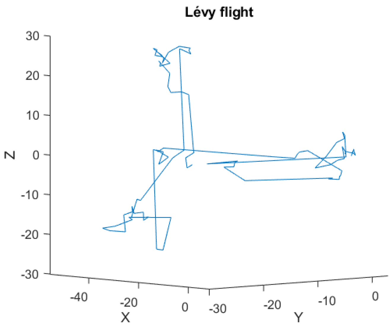
Figure 6 shows an example implementation of a Lévy flight (visualization restricted to

R^{3}

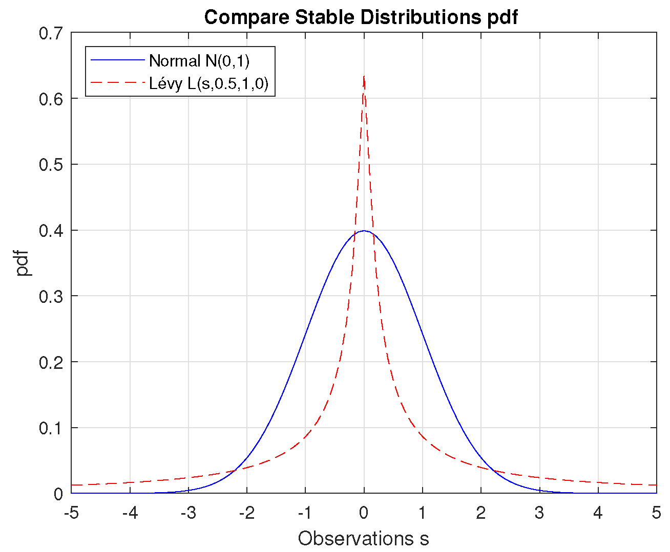
space), with the parameters listed in Table 5. Analyzing the steps generated in the CS algorithm used, it can be seen that among the large number of small steps of the algorithm, from time to time there are large jumps called Lévy flights, after the French mathematician Paul Pierre Lévy. A characteristic feature of this Lévy distribution [21] is the long “tails” that occur for large values – unlike the Gauss (Normal) distribution (Figure 7) [22]. In fact, the trajectory of a Lévy flight has fractal dimension

d_{f} = λ

[23,24,25]. A search for the maximum of the criterion function

F_{c_{1}}

(4) and

F_{c_{4}}

(12) was performed for the two selected algorithms. For each combination of the selected control parameters of the algorithm,

N_{r e p c a l c}

(number of repetitions) calculations were performed (Table 5). The range of control parameters of the algorithms was chosen arbitrarily, limiting them to the most characteristic cases for the considered algorithm. In addition, the calculation parameters for the CS algorithm (number of iterations

N_{i t e r}^{m a x}

and number of repetitions

N_{r e p c a l c}

) were chosen so that the calculation times were comparable.

where:

x_{i}^{b e s t}

- the best solution (nest with the best egg).

5. Calculation Results

For the control variables of the selected algorithms presented in Table 5, obtain results of calculations and solutions for scenario 1 and scenario 2 obtained with the two analyzed algorithms. For the CS [26] algorithm, the calculations concerned changes in the probability of detecting an egg tossed by the cuckoo

p_{a}

and Lévy distribution parameter

λ

(Table 5). For the FA algorithm [27], all combinations of the three parameters listed in Table 5 were considered: randomness

α_{f f}

, reference “attractiveness” factor

β_{0}

and absorption coefficient

γ

. An improvement index is required to measure the improvement of the best solutions found by the FA algorithm in comparison with those given by CS. This index [12], which has been called Maximum Possible Improvement (MPI), is as follows:

M P I (%) = \frac{F_{c}^{F A} - F_{c}^{a l g}}{1 - F_{c}^{a l g}}

(25)

where:

F_{c}^{F A}

F_{c}^{a l g}

—the best system reliability for criteria function

F_{c_{1}}

(Equation (4)) or

F_{c_{4}}

(Equation (12)) obtained by the FA algorithm and other algorithm (

a l g \notin F A

) e.g., CS algorithm.

The correlation coefficient between the results (criterion function values) of the two scenarios using the FA and CS algorithm was calculated according to the formulas:

r^{a l g} = \frac{\sum_{p a r 1, p a r 2, . . .} (F_{c_{1}}^{a l g} - \bar{F_{c_{1}}^{a l g}}) \cdot (F_{c_{4}}^{a l g} - \bar{F_{c_{4}}^{a l g}})}{\sqrt{(\sum_{p a r 1, p a r 2, . . .} {(F_{c_{1}}^{a l g} - \bar{F_{c_{1}}^{a l g}})}^{2})} \cdot \sqrt{(\sum_{p a r 1, p a r 2, . . .} {(F_{c_{4}}^{a l g} - \bar{F_{c_{4}}^{a l g}})}^{2})}},

(26)

where:

\bar{F_{c_{1}}^{a l g}}

\bar{F_{c_{4}}^{a l g}}

—mean value of the criteria function

F_{c_{1}}

(Equation (4)) and

F_{c_{4}})

(Equation (12)) obtained by algorithm (

a l g

) FA or CS,

p a r 1, p a r 2, . . .

parameters algorithms, e.g.,: FA:

α_{f f}, β_{0}, γ

or CS:

p_{a}, λ

To determine the reasonable significant difference of average performance, test statistics of ANalysis Of VAriance (ANOVA) was used. Post hoc (RIR) Tukey test Honest Significant Difference (HSD) was conduced, to investigated which of the parameters are different from each other for tested algorithm.

Presented values (in tables and figures) of criterion functions and constraints are unitless.

5.1. Results for FA

For both scenarios, the best results have been achieved for the FA algorithm parameter set:

α_{f f}

=0.5,

β_{0}

=1.0,

γ

=0.01. For criterion function

F_{c_{1}}

, maximum value was 0.99995661 (Table 6). In scenario 2, the best solutions have been achieved with

F_{c_{4}}

=0.99992902 (Table 7) for FA algorithm.

Table 6. The best solution for scenario 1 for FA.

Parameters	$α_{f f} = 0.5, β_{0} = 1.0$ , $γ$ =0.01
Solutions $F_{c}^{m i n}$	0.99995653
Solutions $F_{c}^{m a x}$	0.99995661
Solutions $F_{c}^{m e a n}$	0.99995657
Solutions $σ$	2.27604463e–08
Calc. time [s]	216.0in

Table 7. The best solution for scenario 2 has been achieved using FA.

Parameters	$α_{f f} = 0.5, β_{0} = 1.0$ , $γ$ =0.01
Solutions $F_{c}^{m i n}$	0.99992644
Solutions $F_{c}^{m a x}$	0.99992902
Solutions $F_{c}^{m e a n}$	0.99992773
Solutions $σ$	9.85429365e–07
Calc. time [s]	189.3

Table 8. The best solution for scenario 2 by FA:

α_{f f} = 0.5, β_{0} = 1.0

γ

=0.01.

Table 8. The best solution for scenario 2 by FA:

α_{f f} = 0.5, β_{0} = 1.0

γ

=0.01.

Parameters	Values	Parameters	Values
$r_{1}$	0.8500	$n_{1}$	4
$r_{2}$	0.8500	$n_{2}$	4
$r_{3}$	0.8500	$n_{3}$	4
$r_{4}$	0.8500	$n_{4}$	4
$r_{5}$	0.8500	$n_{5}$	4
$r_{6}$	0.7429	$n_{6}$	1
$r_{7}$	0.7989	$n_{7}$	2
$r_{8}$	0.6626	$n_{8}$	2
$r_{9}$	0.6902	$n_{9}$	2
$r_{10}$	0.8295	$n_{10}$	2

Table 9. Post-hoc Tuckey RIR tests for FA scenario 1 and

α_{f f}

=0.4,

β_{0}

=0.5 and

γ

=0.1.

Table 9. Post-hoc Tuckey RIR tests for FA scenario 1 and

α_{f f}

=0.4,

β_{0}

=0.5 and

γ

=0.1.

Parameters	p-values
$α_{f f}$ =0.1, $β_{0}$ =0.1, $γ$ =0.01	0.000116
$α_{f f}$ =0.1, $β_{0}$ =0.2, $γ$ =0.01	0.000116
$α_{f f}$ =0.2, $β_{0}$ =0.1, $γ$ =0.01	0.000116
$α_{f f}$ =0.1, $β_{0}$ =0.1, $γ$ =0.1	0.000116
$α_{f f}$ =0.1, $β_{0}$ =0.2, $γ$ =0.1	0.000116
$α_{f f}$ =0.1, $β_{0}$ =0.3, $γ$ =0.1	0.000116
$α_{f f}$ =0.2, $β_{0}$ =0.1, $γ$ =0.1	0.000116
$α_{f f}$ =0.2, $β_{0}$ =0.2, $γ$ =0.1	0.000116
$α_{f f}$ =0.1, $β_{0}$ =0.1, $γ$ =1.0	0.000116
$α_{f f}$ =0.1, $β_{0}$ =0.2, $γ$ =1.0	0.000116
$α_{f f}$ =0.1, $β_{0}$ =0.3, $γ$ =1.0	0.000116
$α_{f f}$ =0.1, $β_{0}$ =0.4, $γ$ =1.0	0.000116
$α_{f f}$ =0.1, $β_{0}$ =0.5, $γ$ =1.0	0.000116
$α_{f f}$ =0.1, $β_{0}$ =0.6, $γ$ =1.0	0.000116
$α_{f f}$ =0.1, $β_{0}$ =0.7, $γ$ =1.0	0.000116
$α_{f f}$ =0.1, $β_{0}$ =0.8, $γ$ =1.0	0.000116
$α_{f f}$ =0.1, $β_{0}$ =0.9, $γ$ =1.0	0.000116
$α_{f f}$ =0.1, $β_{0}$ =1.0, $γ$ =1.0	0.000117
$α_{f f}$ =0.2, $β_{0}$ =0.1, $γ$ =1.0	0.000116
$α_{f f}$ =0.2, $β_{0}$ =0.2, $γ$ =1.0	0.000116
$α_{f f}$ =0.2, $β_{0}$ =0.3, $γ$ =1.0	0.000116
$α_{f f}$ =0.2, $β_{0}$ =0.4, $γ$ =1.0	0.000116
$α_{f f}$ =0.2, $β_{0}$ =0.5, $γ$ =1.0	0.000116
$α_{f f}$ =0.2, $β_{0}$ =0.6, $γ$ =1.0	0.000116
$α_{f f}$ =0.3, $β_{0}$ =0.1, $γ$ =1.0	0.000116
$α_{f f}$ =0.3, $β_{0}$ =0.2, $γ$ =1.0	0.000116
$α_{f f}$ =0.3, $β_{0}$ =0.3, $γ$ =1.0	0.000116
$α_{f f}$ =0.3, $β_{0}$ =0.4, $γ$ =1.0	0.014025
$α_{f f}$ =0.3, $β_{0}$ =0.5, $γ$ =1.0	0.000116
$α_{f f}$ =0.3, $β_{0}$ =0.6, $γ$ =1.0	0.000144
$α_{f f}$ =0.3, $β_{0}$ =0.7, $γ$ =1.0	0.000116

Table 10. Post-hoc RIR Tuckey tests for FA scenario 2 and

α_{f f}

=0.4,

β_{0}

=0.8 and

γ

=0.01.

Table 10. Post-hoc RIR Tuckey tests for FA scenario 2 and

α_{f f}

=0.4,

β_{0}

=0.8 and

γ

=0.01.

Parameters	p-values
$α_{f f}$ =0.1, $β_{0}$ =0.1	0.000047
$α_{f f}$ =0.2, $β_{0}$ =0.1	0.000047
$α_{f f}$ =0.1, $β_{0}$ =0.2	0.000047
$α_{f f}$ =0.1, $β_{0}$ =0.3	0.483894
$α_{f f}$ =0.3, $β_{0}$ =0.7	0.997808
$α_{f f}$ =0.1, $β_{0}$ =0.8	0.857372
$α_{f f}$ =0.2, $β_{0}$ =0.8	0.987661
$α_{f f}$ =0.3, $β_{0}$ =0.8	0.999464
$α_{f f}$ =0.1, $β_{0}$ =0.9	0.991139
$α_{f f}$ =0.2, $β_{0}$ =0.9	0.999796
$α_{f f}$ =0.3, $β_{0}$ =0.9	0.952106
$α_{f f}$ =0.1, $β_{0}$ =1.0	0.278482
$α_{f f}$ =0.2, $β_{0}$ =1.0	0.832396
$α_{f f}$ =0.3, $β_{0}$ =1.0	0.999918
other cases	1.000000

Analysing the parameter space with the ad-hoc RIR Tuckey test (ANOVA), it can be seen that for the set of

α_{f f}

=0.4,

β_{0}

=0.8,

γ

=0.01 parameters, the hypothesis of no reasonable difference should be rejected for three cases.

5.2. Results for CS

Due to different solutions using the CS algorithm (Table 11 and Table 12), the stopping criterion a and the number of iterations have been changed (Table 5).

The solutions for parameter

N_{i t e r}^{m a x}

=1000,

N_{r e p c a l c}

=10000 (Table 13) were also checked.

A more detailed analysis of the parameter space led to the largest values of the criterion function in both scenarios for

α_{f f}

=0.4,

β_{0}

=0.8,

γ

=0.01 and the exact maximum value was

F_{c_{1}}

=0.999956606987731. For the second scenario, the exact maximum value of the criterion function

F_{c_{4}}

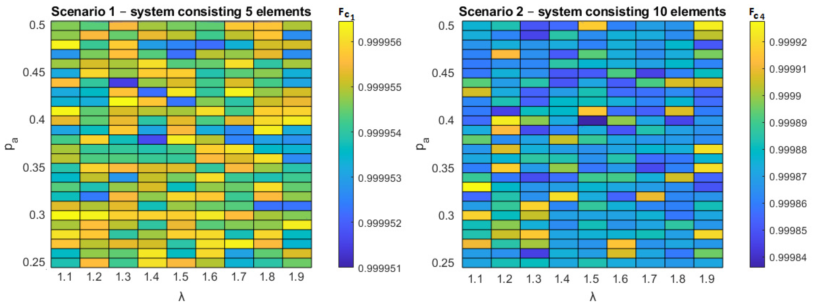
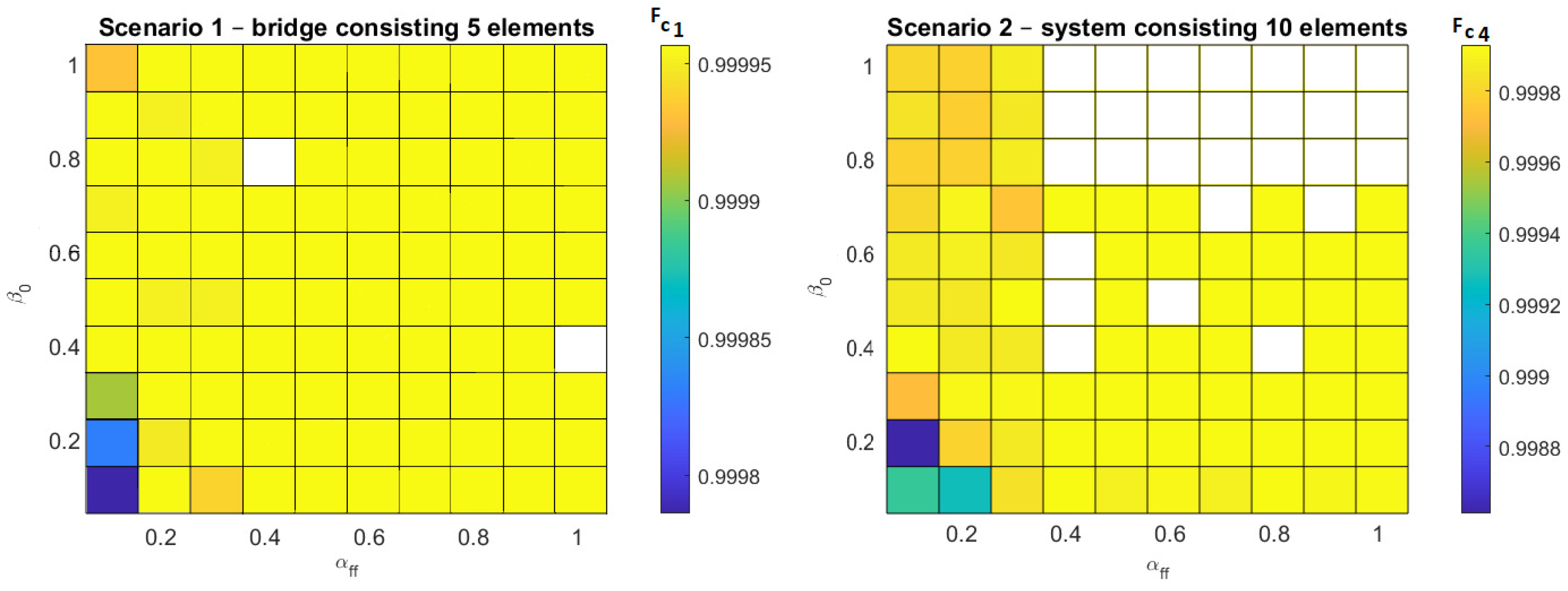
=0.999929024736168 was reached in 28 cases (white boxes Figure 8). By reviewing the control parameter space of the FA algorithm (Figure 9) it is possible to observe a high compliance of the range of algorithm parameters leading to worse solutions. The highest values of correlation r (26) were achieved for (Figure 9):

α_{f f}

=0.5,

r^{F A}

=0.9912,

α_{f f}

=0.7,

r^{F A}

=0.9881 and

α_{f f}

=0.9,

r^{F A}

=0.9858.

By reviewing the control parameter space of the CS algorithm (Figure 8), similar (small value of MPI)—but “worse” solutions can be obtained (Table 13 and Table 15). The highest values of correlation

r^{C S}

(26) were achieved for (Figure 8):

p_{a}

=0.39,

r^{C S}

=0.7855,

p_{a}

=0.25,

r^{C S}

=0.7105 and

p_{a}

=0.30,

r^{C S}

=0.6264.

For the first scenario, the usage of FA led to (Table 6) to better results (compared to the results for the CS), but use of the CS cuckoo algorithm led to a solution in much less time consumed (Table 16). All calculations were performed using Matlab package R2020b (also with Statistic and Machine Learning Toolbox) on Win 10 pro operating system and Intel(R) Core(TM) i5–7200U CPU @ 2.50GHz. The solutions obtained using the CS algorithm were different from those obtained using FA algorithm, for example the number of elements

(n_{3} \div n_{5})

(Table 11 vs. Table 12) for scenario 1, number of elements (

n_{5}

) Table 8 vs. Table 17) for scenario 2 and of course values the reliability. In the investigated space of FA control parameters, difficulties in obtaining a solution satisfying the assumed constraints occurred in both scenarios for the set

α_{f f}

=0.1;

β_{0}

=1.0;

γ

=0.1, and additionally for second scenario

α_{f f}

=0.1,

β_{0}

=0.5,

γ

=0.1. In addition, the effect of changing the lambda parameter (

λ

) of the Lévy distribution on the solutions achieved was checked with an increased number of iterations (Table 5). For the CS algorithm (first scenario), it led to the highest value of the criterion function for the parameters –

p_{a}

= 0.27,

λ = 1.5

N_{i t e r}^{m a x}

=100,

N_{r e p c a l c}

=10 (Table 16) and

p_{a}

= 0.30,

λ

=1.1 for

N_{i t e r}^{m a x}

=1000,

N_{r e p c a l c}

=10000 (Table 13). Increasing the number of iterations

N_{i t e r}^{m a x}

and iterations of the algorithm

N_{r e p c a l c}

in scenario no. 1, not only increased the value of the criterion function but also reduced the Euclidean difference (

∥ r^{F A} - r^{C S} ∥_{2}

∥ n^{F A} - n^{C S} ∥_{2}

) to the best solution obtained with the FA algorithm (Table 16 and Table 13). For the second scenario, the highest value of the criterion function, for the CS algorithm, was achieved for

p_{a}

= 0.33,

λ

=1.1 (Table 15). Comparing the solutions, despite the small difference in MPI (Table 7 and Table 15), different values for the sought variables were achieved (Table 8 and Table 17).

6. Conclusions

The presented results broaden the existing discussion on the application of nature-inspired algorithms for solving RRAP problems. From this point of view, two described test scenarios (and the Firefly Algorithm FA) can be considered as a suitable tool for validating other algorithms in RRAP problems. Although the CS algorithm is known for its effectiveness as it uses the Lévy flight (Figure 6), the FA firefly algorithm in the considered parameter range proved to be more effective. The use of the FA algorithm led to solutions with a higher value of the criterion function (Table 6 and Table 7). It can also be notices that the best solutions using CS were achieved for

λ

values different from the 1.5 - as default value (

α = 0.5

) for Lévy stable distribution used. It is worth noting that in both scenarios using the FA algorithm, the sigma value

σ

(standard deviation) was smaller than the solutions using CS.

Not only the values of the criterion functions can be compared, but also the MPI (Equation (25)), the Euclidean distance differences of both the reliability (

∥ r^{F A} - r^{C S} ∥_{2}

) and the number of redundant elements (

∥ n^{F A} - n^{C S} ∥_{2}

) obtained by carefully selecting the parameters of the CS algorithm.

The comparison of the values of the criterion function, the linear r-Pearson correlation coefficient and the data from the post-hoc RIR Tuckey test leads to the selection of the same (or similar) control parameters of the analysed algorithms. Therefore, the presented analysis methods can also be used to compare other optimization algorithms.

Such an approach can broaden the application the well-known test function benchmarks for global in the RRAP optimization (test functions e.g.: Michalewicz’s, Rosenbrock’s, De Jong’s, Schwefel’s, Ackley’s, Rastring’s, Easom’s, Griewank’s, Shubert’s [18,28], Bohachenoticed Matyas’s, Zakharov’s, Goldstein-Prices [29], other functions [30,31] or other Tallard’s test functions [32]). From the compilation of literature data [3,4], the use of algorithms: PSO, MPSO, ABC, CS–GA, BAT, ACO led to obtaining worse solutions than FA. The question remains open: are other algorithms lead to obtaining a different global maximum of the considered (or other RRAP) criterion functions?

Author Contributions

A.P. and B.F. equally contributed in all stages of the project. Conceptualization, A.P. and B.F.; methodology, A.P. and B.F.; software, A.P.; validation, A.P. and B.F.; formal analysis, A.P.; investigation, A.P. and B.F.; resources, B.F.; data curation, A.P.; writing—original draft preparation, A.P.; writing—review and editing, A.P. and B.F.; visualization, A.P.; supervision, B.F.; project administration, A.P. All authors have read and agreed to the published version of the manuscript. All authors reviewed the manuscript.

Funding

This research received no external funding.

Informed Consent Statement

Not applicable.

Data Availability Statement

Not applicable.

Conflicts of Interest

The authors declare no conflict of interest.

Sample Availability

Samples of the compounds ... are available from the authors.

Abbreviations

The following abbreviations are used in this manuscript:

RRAP	Reliability Redundancy Allocation Problem
CS	Cuckoo Search
FA	Firefly Algorithm

References

Sobczak, W. Podstawy Probabilistyczne Teorii SystemóW Informacyjnych; WNT: Warsaw, Poland, 1981. [Google Scholar]
Yang, X.S. Nature-Inspired Optimisation Algorithms; Elsevier, 2014. [CrossRef]
Yang, X.S. Multiobjective firefly algorithm for continuous optimization. Eng. Comput. 2013, 29, 175–184. [Google Scholar] [CrossRef]
Kwiecień, J.; Filipowicz, B. Optymalizacja niezawodności zlozonych systemẃ za pomoca algorytmu świetlika. Eksploat. Niezawodn. Maint. Reliab. 2017, 19, 296–301. [Google Scholar] [CrossRef]
Kwiecień, J. Algorytmy stadne w rozwiazaniu wybranych zagadnień optymalizacji dyskretnej i kombinatorucznej; AGH: Cracow, Poland, 2015. [Google Scholar]
Klempka, R.; Filipowicz, B. Comparison of using the genetic algorithm and cuckoo search for multicriteria optimisation with limitation. Turk. J. Electr. Eng. Comput. Sci. 2017, 25, 1300–1310. [Google Scholar] [CrossRef]
Zhao, K.; Jurdak, R.; Liu, J.; Westcott, D.; Kusy, B.; Parry, H.; Sommer, P.; McKeown, A. Optimal Levy-flight foraging in a finite landscape. J. R. Soc. Interface R. Soc. 2015, 12. [Google Scholar] [CrossRef] [PubMed]
Fuksa, A.K. Zastosowanie sztucznej inteligencji w optymalizacji niezawodnościowej systemów. PhD Thesis, AGH Akademia Górniczo-Hutnicza, Kraków, 2017. [Google Scholar]
Kuo, S.; Yeh, F.; Lin, H. Efficient and Exact Reliability Evaluation for Networks With Imperfect Vertices. IEEE Trans. Reliab. 2007, 56, 288–300. [Google Scholar] [CrossRef]
Kuo, S.Y.; Lu, S.K.; Yeh, F.M. Determining terminal-pair reliability based on edge expansion diagrams using OBDD. IEEE Trans. Reliab. 1999, 48, 234–246. [Google Scholar] [CrossRef]
Yeh, F.M.; Lu, S.K.; Kuo, S.Y. OBDD-based evaluation of k-terminal network reliability. IEEE Trans. Reliab. 2002, 51, 443–451. [Google Scholar] [CrossRef]
Valian, E. Solving Reliability Optimization Problems. In Cuckoo Search and Firefly Algorithm Theory and Applications; Yang, X.S., Ed.; Springer: London, 2014; pp. 195–216. [Google Scholar]
Pijarski, P. Optymalizacja heurystyczna w ocenie warunków pracy i planowania rozwoju systemu elektroenergetycznego; Politechnika Lubelska: Lublin, Poland, 2019. [Google Scholar]
R., D.; V., K. Power system oscillation damping controller design: A novel approach of integrated HHO-PSO algorithm. Arch. Control. Sci. 2021, 31, 553–591. [Google Scholar] [CrossRef]
Kusiak, J.; Danielewska-Tułecka, A.; Oprocha, P. Optymalizacja Wybrane metody z przykladami zastosowań; PWN: Warsaw, Poland, 2009. [Google Scholar]
Filipowicz, B.; Kwiecień, J. Algorytmy stadne w problemach optymalizacji. Pomiary Autom. Robot. 2011, 15, 152–157. [Google Scholar]
Fuksa, K. Zastosowanie sztucznej inteligencji w optymalizacji niezawodnościowej systemów. PhD Thesis, AGH, AGH Cracow, Poland, 2017. [Google Scholar]
Yang, X.S.; Deb, S. Cuckoo Search via Levy Flights 2010.
Vázquez, R.; Sandoval, G.; Ambrosio Bastian, J. How to Generate the Input Current for Exciting a Spiking Neural Model Using the Cuckoo Search Algorithm; 2014; Vol. 516, pp. 155–178. [CrossRef]
Manteng, R. Fast, accurate algorithm for numerical simulation of Levy stable stochastic process. Phys. Rev. E 1994, 5, 4677–4683. [Google Scholar] [CrossRef] [PubMed]
Viswanathan, G.; Afanasyev, V.; Buldyrev, S.V.; Havlin, S.; da Luz, M.; Raposo, E.; Stanley, H. Lévy flights in random searches. Phys. A Stat. Mech. Its Appl. 2000, 282, 1–12. [Google Scholar] [CrossRef]
Nolan, J. Stable Distributions: Models for Heavy-Tailed Data; Springer: New York, NY, USA, 2016. [Google Scholar]
Hughes, B. Random Walks and Random Environments: Random walks; Number t. 1 in Oxford science publications, Clarendon Press, 1995.
Chechkin, A.; Metzler, R.; Klafter, J.; Gonchar, V., Introduction to the Theory of Lévy Flights; 2008; pp. 129 – 162. [CrossRef]
Bovet, A. An Introduction to Non-diffusive Transport Models. ArXiv 2015. [Google Scholar] [CrossRef]
Yang, X.S. Website of the: Cuckoo Search (CS) Algorithm, MATLAB Central File Exchange. 2020. Available online: https://www.mathworks.com/matlabcentral/fileexchange/29809-cuckoo-search-cs-algorithm (accessed on ).
Yang, X.S. Website of the: Firefly Algorithm, MATLAB Central File Exchange. 2021. Available online: https://www.mathworks.com/matlabcentral/fileexchange/29693-firefly-algorithm (accessed on ).
Roy, S.; Chaudhuri, S. Cuckoo Search Algorithm using Lèvy Flight: A Review. Int. J. Mod. Educ. Comput. Sci. 2013, 5, 10–15. [Google Scholar] [CrossRef]
Mareli, M.; Twala, B. An adaptive Cuckoo search algorithm for optimisation. Appl. Comput. Inform. 2017, 14. [Google Scholar] [CrossRef]
Yang, X.S. (Ed.) Nat.-Inspired Optim. Algorithms; Elsevier: Oxford, 2014; p. i. [Google Scholar] [CrossRef]
Surjanovic, S.; Bingham, D. Virtual Library of Simulation Experiments: Test Functions and Datasets. Available online: http://www.sfu.ca/ssurjano (accessed on 31 December 2022).
Taillard, E. Benchmarks for basic scheduling problems. Eur. J. Oper. Res. 1993, 64, 278–285. [Google Scholar] [CrossRef]

Figure 1. The schematic diagram of an overspeed system for a gas turbine [12].

Figure 2. Diagram of the bridge system analysed in scenario 1.

Figure 3. System reliability for different analysis methods with n=1 (set fixed number of redundant elements).

Figure 4. Analysis of the second constraint

g_{2}

(r,n).

Figure 4. Analysis of the second constraint

g_{2}

(r,n).

Figure 5. Diagram of the 10 elements system under analysis in scenario 2.

Figure 6. Visualization of an example Lévy flight (

λ

=1.3) in Euclidean space

R^{3}

Figure 6. Visualization of an example Lévy flight (

λ

=1.3) in Euclidean space

R^{3}

Figure 7. Compare Stable Distributions pdf.

Figure 8. Solutions for scenario 1 and 2 has been achieved using CS algorithm.

Figure 9. Solutions for scenario 1 and 2 has been achieved using FA algorithm for parameter

γ

=0.01.

Figure 9. Solutions for scenario 1 and 2 has been achieved using FA algorithm for parameter

γ

=0.01.

Table 1. Bridge system settings.

$β_{i}$	V	C	W	T [h]
1.5	110	175	200	1000

Table 2. Bridge system settings.

Subsystem i	$10^{5} \cdot α_{i}$	$w_{i} \cdot v_{i}^{2}$	$w_{i}$
1	2.330	1	7
2	1.450	2	8
3	0.541	3	8
4	8.050	4	6
5	1.950	2	9

Table 3. Parameters used in scenario 2.

i	$c_{1 i}$	$c_{2 i}$	$c_{3 i}$	$c_{4 i}$	$c_{5 i}$
1	33.2468	35.6054	13.7848	44.1345	10.9891
2	27.5668	44.9520	96.7365	25.9855	68.0713
3	13.3800	28.6889	85.8783	19.2621	1.0164
4	0.4710	0.4922	63.0815	12.1687	29.4809
5	51.2555	39.6833	78.5364	23.9668	59.5441
6	82.9415	59.2294	11.8123	28.9889	46.5904
7	51.8804	78.4996	97.1872	47.8387	49.6226
8	77.9446	86.6633	45.0850	25.0545	59.2594
9	26.8835	7.8195	3.6722	76.9923	87.4070
10	85.8722	27.7460	55.3950	53.3007	55.3175

Table 4. Parameters used in scenario 2.

Parameters	$d_{r a n d}$
$c_{1 i}$	3.1250
$c_{2 i}$	3.4710
$c_{3 i}$	3.3247
$c_{4 i}$	2.6236
$c_{5 i}$	3.4288

Table 5. Parameters of scenario 1 and scenario 2.

Parameters	Values
Problem dimension	$N_{D}$ = $m_{s c} \cdot 2$ ; sc $\in {1, 2}$ ; $m_{1}$ =5, $m_{2}$ =10
Maximum number of iterations	$N_{i t e r}^{m a x}$ = 100 and 1000 (CS)
Number of repetitions (each case)	$N_{r e p c a l c}$ =10 and 10000 (CS)
Constraints values (lower bound, upper bound)	$l b_{1}$ =0.65; $u b_{1}$ =0.85; $l b_{2}$ =1; $u b_{2}$ =4
CS – Cuckoo Search Algorithm
Number of nests	$N_{n e s t s}$ = 50
Probability of detecting a cuckoo’s egg	$p_{a} = {0.25, 0.26, \dots, 0.50}$
Lévy distribution parameter	$λ = {1.1, 1.2, \dots, 1.9}$
Positive step size scaling factor	$α_{C S} = \frac{1}{100} \cdot N (0, 1) \cdot (x_{i}^{k - 1} - x_{i}^{b e s t})$
FA – Firefly Algorithm
Number of fireflies	$N_{f f}$ = 50
Randomization parameter	$α_{f f} = {0.1, 0.2, \dots, 1.0}$
Reference factor of ’attractiveness’	$β_{0} = {0.1, 0.2, \dots, 1.0}$
Absorption coefficient	$γ = {0.01, 0.10, 1.00}$

Table 11. The best solution for scenario 1 by FA

α_{f f} = 0.5, β_{0} = 1.0

γ

=0.01.

Table 11. The best solution for scenario 1 by FA

α_{f f} = 0.5, β_{0} = 1.0

γ

=0.01.

Parameters	Values
$r_{1}$	0.78571
$r_{2}$	0.8500
$r_{3}$	0.8500
$r_{4}$	0.7520
$r_{5}$	0.6601
$n_{1}$	4
$n_{2}$	4
$n_{3}$	3
$n_{4}$	2
$n_{5}$	3

Table 12. The best solution for scenario 1 by CS:

p_{a}

=0.27,

λ = 1.5

N_{i t e r}^{m a x} = 100, N_{r e p c a l c} = 10

Table 12. The best solution for scenario 1 by CS:

p_{a}

=0.27,

λ = 1.5

N_{i t e r}^{m a x} = 100, N_{r e p c a l c} = 10

Parameters	Values
$r_{1}$	0.8298
$r_{2}$	0.8380
$r_{3}$	0.8500
$r_{4}$	0.6500
$r_{5}$	0.7265
$n_{1}$	4
$n_{2}$	4
$n_{3}$	2
$n_{4}$	3
$n_{5}$	2

Table 13. The best solution for scenario 1 by CS.

Parameters	$p_{a}$ =0.30, $λ = 1.1$
	$N_{i t e r}^{m a x} = 1000, N_{r e p c a l c} = 10000$
Solutions $F_{c}^{m i n}$	0.99921071
Solutions $F_{c}^{m a x}$	0.99995645
Solutions $F_{c}^{m e a n}$	0.99984281
Solutions $σ$	6.41364325e–05
Calc. time [s]	346.4
MPI (%)	0.0037
$∥ r^{F A} - r^{C S} ∥_{2}$	0.0124
$∥ n^{F A} - n^{C S} ∥_{2}$	0

Table 14. The best solution for scenario 1 by CS:

p_{a}

=0.30,

λ = 1.1

N_{i t e r}^{m a x} = 1000, N_{r e p c a l c} = 10000

Table 14. The best solution for scenario 1 by CS:

p_{a}

=0.30,

λ = 1.1

N_{i t e r}^{m a x} = 1000, N_{r e p c a l c} = 10000

Parameters	Values
$r_{1}$	0.7919
$r_{2}$	0.8500
$r_{3}$	0.8499
$r_{4}$	0.7483
$r_{5}$	0.6500
$n_{1}$	4
$n_{2}$	4
$n_{3}$	3
$n_{4}$	2
$n_{5}$	3

Table 15. The best solution for scenario 2 by CS.

Parameters	$p_{a}$ =0.33, $λ = 1.1$
	$N_{i t e r}^{m a x} = 1000, N_{r e p c a l c} = 10000$
Solutions $F_{c}^{m i n}$	0.99550799
Solutions $F_{c}^{m a x}$	0.99992758
Solutions $F_{c}^{m e a n}$	0.99892402
Solutions $σ$	5.51629947e-04
Calc. time [s]	387.5
MPI (%)	0.0198
$∥ r^{F A} - r^{C S} ∥_{2}$	0.1893
$∥ n^{F A} - n^{C S} ∥_{2}$	1

Table 16. The best solution for scenario 1 by CS.

Parameters	$p_{a}$ =0.27, $λ = 1.5$
	$N_{i t e r}^{m a x} = 100, N_{r e p c a l c} = 10$
Solutions $F_{c}^{m i n}$	0.99972966
Solutions $F_{c}^{m a x}$	0.0.99994780
Solutions $F_{c}^{m e a n}$	0.99984451
Solutions $σ$	7.40185829e–05
Calc. time [s]	1.7
MPI (%)	0.1688
$∥ r^{F A} - r^{C S} ∥_{2}$	0.1300
$∥ n^{F A} - n^{C S} ∥_{2}$	1.7321

Table 17. The best solution for scenario 2 by CS:

p_{a}

=0.33,

λ = 1.1

N_{i t e r}^{m a x} = 1000, N_{r e p c a l c} = 10000

Table 17. The best solution for scenario 2 by CS:

p_{a}

=0.33,

λ = 1.1

N_{i t e r}^{m a x} = 1000, N_{r e p c a l c} = 10000

Parameters	Values	Parameters	Values
$r_{1}$	0.8500	$n_{1}$	4
$r_{2}$	0.8500	$n_{2}$	4
$r_{3}$	0.8500	$n_{3}$	4
$r_{4}$	0.8500	$n_{4}$	4
$r_{5}$	0.8500	$n_{5}$	3
$r_{6}$	0.7671	$n_{6}$	1
$r_{7}$	0.8453	$n_{7}$	2
$r_{8}$	0.8432	$n_{8}$	2
$r_{9}$	0.6973	$n_{9}$	2
$r_{10}$	0.8500	$n_{10}$	2

Disclaimer/Publisher’s Note: The statements, opinions and data contained in all publications are solely those of the individual author(s) and contributor(s) and not of MDPI and/or the editor(s). MDPI and/or the editor(s) disclaim responsibility for any injury to people or property resulting from any ideas, methods, instructions or products referred to in the content.

© 2023 by the authors. Licensee MDPI, Basel, Switzerland. This article is an open access article distributed under the terms and conditions of the Creative Commons Attribution (CC BY) license (http://creativecommons.org/licenses/by/4.0/).

Copyright: This open access article is published under a Creative Commons CC BY 4.0 license, which permit the free download, distribution, and reuse, provided that the author and preprint are cited in any reuse.

MDPI Initiatives

Important Links

Choose an area of interest and we will send you notifications of new preprints at your preferred frequency.

Disclaimer

Application of RRAP Reliability Optimization as Test of Nature Inspired Algorithms

Abstract

1. Introduction

2. Problem Definition

3. Models of the RRAP System

3.1. Scenario 1—Bridge System

3.2. Scenario 2—System Consisting 10 Elements

4. Selected Optimization Algorithms

4.1. Firefly Algorithm FA

4.2. Cuckoo Search CS

5. Calculation Results

5.1. Results for FA

5.2. Results for CS

6. Conclusions

Author Contributions

Funding

Informed Consent Statement

Data Availability Statement

Conflicts of Interest

Sample Availability

Abbreviations

References

MDPI Initiatives

Important Links

Subscribe