1. Introduction
Artificial intelligence (AI) is becoming more and more part of our lives. There have been great advances recently in an AI subfield called machine learning (ML). In particular, many-layered neural networks (i.e., deep learning) have brought us technological wonders. Facial recognition allows us to conveniently protect our smart phones (e.g. [
1]). Natural language processing models understand human speech and turn it into commands for smart home applications [
2]. Companies also use AI extensively in industrial applications ranging from the interpretation of infrared images of machinery [
3] to the analysis of process plant data [
4]. There is a strong competition to improve performance which leads to larger models that are trained longer. This in turn implies a greater energy consumption (cf. [
5], [
6] and [
7]).
Yet, as concern over the climate crisis increases, more thought is given to the carbon footprint of AI models. Current models grow in size and start to consume energy on a massive scale for training alone. Critics of this trend cite examples such as GPT-3 [
2], a deep NLP model with 175B parameters that writes human-like texts and needed 1’287 MWh for training. This corresponds to 552 t of CO
2, which is equal to the annual emission of 276 average-style cars [
6]. On the other hand, Patterson et al feel that some studies exaggerate the scope of the problem (cf. [
8]). Also, in our experience, not all models are even near that size. In the end, many AI users are not sure what their models’ carbon footprint is and how to reduce it.
In this paper, after a brief review of related work, we explain what the main drivers of a deep learning model’s carbon footprint are and how they are influenced by different decisions at various stages of the model life cycle (section 0). As a step towards an empirical verification of this model, we explore the footprint of different AI models based on experiments and extrapolations in section 0. We conclude with a critical analysis of the findings and their relevance for developers of AI models who are not at the cutting edge of research.
Our main contributions in this paper are two-fold. First, we provide a consolidated life cycle model to consistently understand the drivers of deep learning’s carbon footprint. Second, we show the results of a series of experiments that test the key claims found in the literature. This allows us to provide a well-founded view on how much of a problem AI carbon footprint is today and how to address this issue. While we need to go into some technical details, we try to keep the paper accessible for readers with a focus on sustainability and no technical background in ML.
2. Related Work
There is already a body of related work that has analyzed potential drivers for the carbon footprint of AI models with a focus on the most expensive kind, i.e., deep learning models. In this section, we start with a definition of scope before looking at the three categories of related work. Our categories are partially inspired by the taxonomy created by García-Martín et al. [
9]. First, we review theoretical calculation models that can be used
ex ante to estimate the cost of architectural decisions. Second, we examine empirical studies on the impact of ML. Finally, we discuss software tools for measuring carbon footprint
ex post, i.e., carbon accounting [
10] after the fact. Obviously, this is not a strict separation, e.g., software tools often use model-based assumptions, and many models are combined with empirical experiments for verification. Thus, the same paper might appear in two or more categories.
2.1. Similar Topics Outside the Scope of this Paper
This paper focuses on the carbon footprint of deep learning models. It does not include other machine learning algorithms such as Support Vector Machines (see [
11] for an analysis) for two reasons. First, the wider the scope, the harder it is to find general statements that are still meaningful decision support. Second, we believe that these models do not have a comparable carbon footprint as deep learning models due to their smaller size and complexity. For similar reasons, generic software assessment standards like Software Carbon Intensity (SCI) [
12] and generic simulation tools such as Wattch [
13] are beyond our scope.
Also, we focus mainly on software-related decisions and designs. While some of the approaches described in the related work rely on specific hardware interfaces, we do not dwell deeply into questions closely related to hardware level analysis or specialized measurement hardware such as MARCHER [
14].
Also unrelated is the use of AI for sustainability tasks. This field of research is sometimes called computational sustainability and “encompasses research on computational contributions to decision making that affects environmental and societal sustainability” [
15]. These algorithms are of particular interest in an industrial environment [
16]. For some general examples see [
7].
2.2. Metrics and Theoretical Models
Theoretical models can be applied ex ante to predict the energy use of a neural network before it is executed. These mathematical models are typically based on specific metrics that can be used as input values.
Several papers have identified the metrics and key drivers behind an ML model’s carbon footprint (see [
6], [
7], [
17], and [18]). These metrics form a good basis for theoretical estimation models but also for software tools and decision support. We use some of these metrics in section 0 where we also discuss those metrics we did not use. For example, a very tempting metric is the number of mathematical operations, i.e., FLOPs [
7] but the connection to energy use is not totally clear-cut (cf. [
19]). Other authors stress the importance of memory access over computation [
20]. Gupta argues that simple metrics (“
single dimensional metrics”) are inherently dangerous are they can lead to false decisions [
21].
A few papers address the energy use of Convolutional Neural Networks (CNNs). Yang et al propose “an energy estimation methodology that can estimate the energy consumption of a DNN based on its architecture, sparsity, and bitwidth” [
20]. Their method focuses on estimations for convolutional and dense layers since these dominate most modern models [
20]. Cai et al propose a predictive framework for CNNs that can be used to estimate the energy use of those models with a learning-based polynomial regression approach. Their model considers the different energy consumptions of different types of layers [
22].
2.3. Empirical Studies
A series of empirical studies on the carbon impact of ML models have been conducted. Wang et al have benchmarked popular AI accelerators (e.g. Intel CPU, NVIDIA GPUs, and Google TPUs) with regard to performance and energy efficiency. The results are complex and not easily translated into rules of thumb [
23]. Lottik et al have compared the energy use of several machine learning models (including a lot of non-neural networks) in their paper [
11]. Yuxing et al have conducted a benchmark study to determine the energy performance of different processors including GPUs and TPUs [
23]. Selvan et al have done a study to determine the energy use of medical image segmentation models [
24]. Finally, Heim et al have studied empirically how different techniques to reduce a models footprint impact, amongst other things, model energy use [
25].
2.4. Software
There are several software tools, which allow measuring the carbon footprint of a model either during execution or afterwards. There are certain key requirements for a good carbon accounting tool. In particular, they need to seamlessly integrate with the development process [
10], provide common, comparable metrics (see [
10] and [
26]), the ability to verify the results [
10], and actionable insights [
10].
Some tools are web-based and use key metrics such as training time, energy mix, and hardware information to estimate the carbon footprint of a model. One example in this category is
ML Emissions Calculator (see [
17] for details). The
Green Algorithms Tool1 is another web-based solution that takes a few key metrics to calculate the carbon footprint of software. Its inputs are runtime, number of CPUs and cores, CPU model, memory, and location. There is also the option to provide information on the data center’s computational overhead (i.e., the PUE, see section 0) as well as some other details. The algorithms behind the software are detailed in a paper [
27].
Other tools integrate directly with the ML code. The python package
energyusage2 (cf. [
11]) contains code that can be called for a Python function and passes a given set of parameters. It computes an estimate of energy use as well as the carbon emissions based on the energy mix of the region where the code is assumed to be run. CPU power usage is computed using the RAPL (Running Average Power Limit) interfaces found on Intel processors. Vendor data is used to make an estimate for computations run on the GPU.
Another tool to evaluate Python code in this fashion is
codecarbon, described in [
6]. Python code is evaluated for its energy use and resulting emissions. For the evaluation, two function calls are needed – one that starts the analysis and one that stops it. The advantage over
energyusage described above is that this way of coding is probably easier to add to existing scripts.
Codecarbon was used in the experiments done for this paper.
The
experiment-impact-tracker3 framework for tracking real-time energy consumption uses a large set of metrics to get a precise energy consumption estimate [
28]. The calculations are based on metrics extracted with Intel’s RAPL or PowerGadget Tool (CPU and DRAM power consumption) and Nvidia’s nvidia-smi (GPU power consumption). The tool also considers processor utilization by the ML algorithm (via psutil and nvidia-smi) and reduces the energy consumption accordingly.
While most software is either system-agnostic or designed for Python, Mohit etl al provide a profiler and tuner for Java. The software is realized as an Eclipse plugin called JEPO [
29].
3. Drivers of Deep Learning AI Models’ Carbon Footprints
The models found in the related work either focus on specific stages of the model lifecycle or are quite abstracted from the actual model properties. Based on the prior art, we propose a comprehensive model that combines and harmonizes the existing models. Our model is based on basic carbon accounting principles, which are described in the first subsection. Next, the ML lifecycle model is proposed. We reexamine the model’s underlying assumptions in the last subsection.
3.1. Fundamental Principle of AI Carbon Footprint
Papers on the climate impact of AI use a variety of special terms that might not be familiar to all readers. In this section, some of these basic terms are explained.
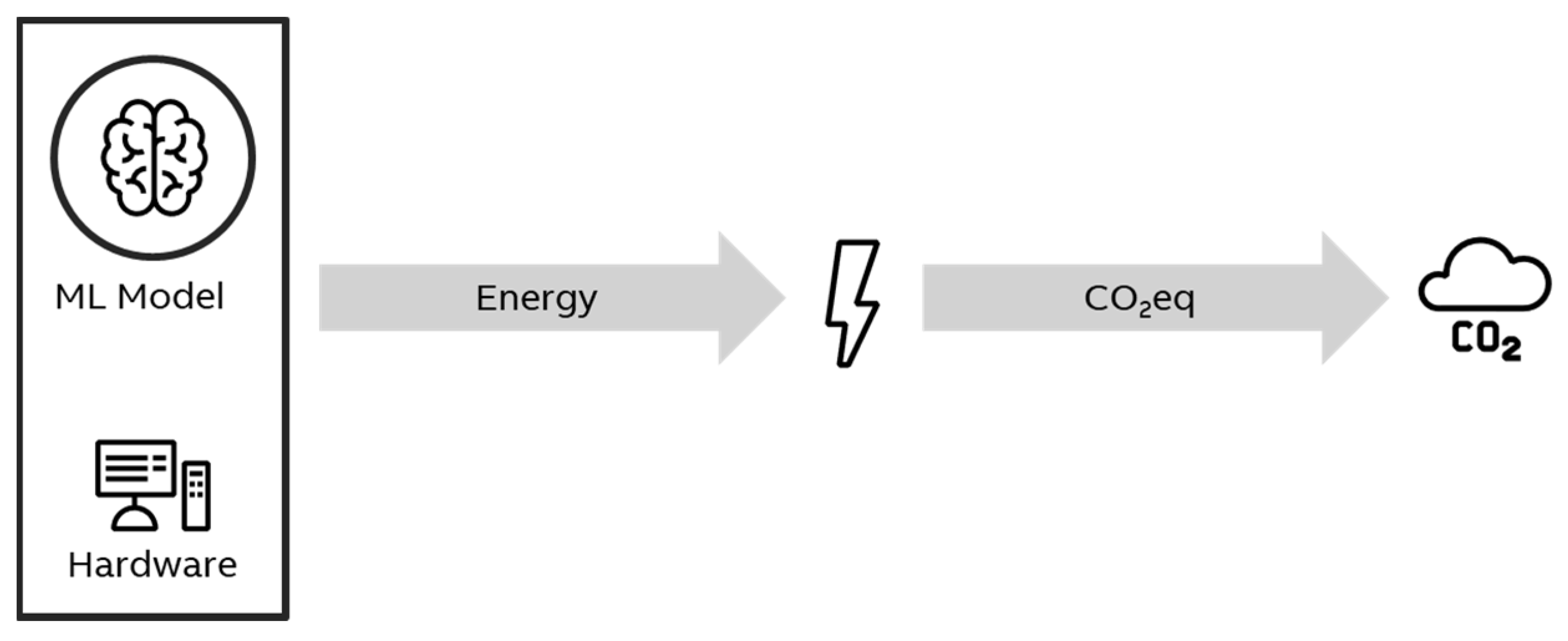
The underlying mechanism behind the carbon footprint of AI/ML models is shown in
Figure 1. Whenever code related to the model is executed, whether for training or as an application (i.e., inference), energy is used. The production of energy can cause CO
2 emissions. From the standpoint of our analysis, AI models cause a carbon footprint corresponding to their energy use. Since this CO
2 might be emitted miles away and at an earlier time, the climate impact of AI models cannot be measured directly, e.g., with some sensor. Instead, it is estimated based on some key “climate drivers” discussed below.
Power is the rate, per unit of time, at which electrical energy is transferred by an electric circuit. Static Power indicates the power consumption without computation, i.e., the base value needed to allow computation to start at any moment. Dynamic Power is the additional power consumption due to computation [
9]. Energy (measured in Joule or kilowatt-hours) is a cumulative value that describes the power used over time.
Using energy as an intermediate input value, the climate impact of an AI model can be calculated. Carbon Intensity describes the amount of CO
2 emitted for the energy consumed [
28]. This value depends on the types of power plants supplying the grid. Mostly renewable energies will have a low carbon intensity. Fossil fuel-based plants have a high carbon intensity.
Power, time, and carbon intensity yield the
CO2eq. This measure describes the climate impact (“carbon footprint”,
Figure 2) of a specific activity in a standardized form and can be used as an indicator to make different ML approaches comparable [
17]. In the context of this paper CO
2eq is practically equivalent to the CO
2 emitted during the production of energy used to power ML algorithms. (It can also describe the impact of other greenhouse gases such as methane.) A related monetary value not used here is
SC-CO2, a measure that quantifies the long-term damage in dollars
4.
3.2. Examples of Neural Network Energy Consumption
At this point, we should mention at what scale the problem discussed in this paper occurs. As has been mentioned before, cutting-edge models such as GTP-3 (with 175B parameters) have a huge carbon footprint – 552t CO
2eq for training alone [
6]. Another NLP model, NAS, is estimated to have used between 415.4 MWh (see table below) and 656.3 MWh [
18] for training. However, these models are not necessarily representative of the common practice [
17].
Table 1 shows some examples of model training carbon footprint. All of these models can be used for real applications, some of them quite complex, such as medical image segmentation. However, not all models have a prohibitive carbon footprint. In fact, most of them have a negligible impact when compared to a single car (avg. 11’000 lbs per year).
3.3. Consolidated Model for AI Carbon Footprint
In Section 0, several carbon footprint models were cited. We feel that all these models only cover aspects of the complete mechanisms or are too high level to be used to predict a model’s impact. In this section, we create a composite model that allows users to estimate the consequences of their modeling decisions ex ante. While the best way to determine a model’s carbon footprint is measurement, this option is only available ex post, so a theoretical model is quite important as well to make the right decisions.
The overall concept presented in
Figure 1 needs to be applied to different distinct phases of the ML life cycle. The three steps are shown below in
Figure 3 (cf. [
6], [
7]). While individually, the first two steps are the most energy-consuming, inference is executed many times in the field and is estimated to cause 80-90% of a model’s total energy use (see [
6], [
30], or [
31] and also consider section 0 to form your own opinion). The next sections describe energy consumption models for each life cycle stage that are based on observations made in the prior art. After that, we explain how to convert the energy consumption to CO
2eq and discuss the limitations of the proposed model.
3.4. Inference
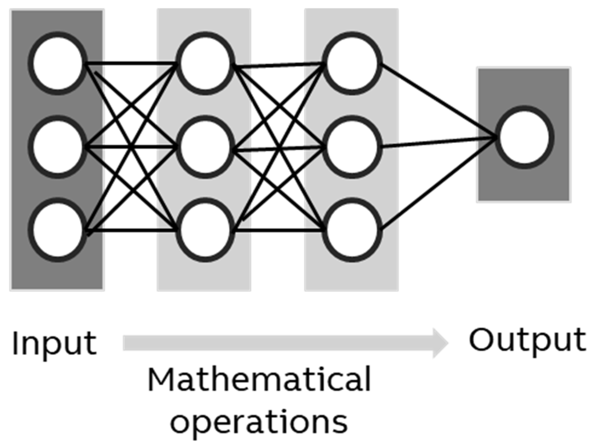
Inference is the “usage stage” of a model and thus the last life cycle stage in ML. However, since the other steps perform test inferences to optimize various parameters, the energy use of inference needs to be explained first. For an inference (
Figure 4), the model takes a single set of data, applies computations, and returns one or more values. These values can be interpreted as new data (e.g., an extrapolation of a value or an image) or as a classification (true/false or multiple classes). For example, when a model is used to detect a fire in a photo, the input is a bitmap and the output is a number that is 1 if there is a fire and 0 if not.
In the simplest case (i.e., a model consisting only of dense layers, the most basic of all layer types), the mathematical operations consist of a series of matrix multiplications as well as the application of a simple activation function such as ), which is called ReLu. Thus, an inference can be described as a series of mathematical operations each of which needs a certain amount of energy.
Inference energy use depends on the model architecture (M) as well as the processing unit type and quantity (
PT). ML can be run on different processors, the main types being CPUs, GPUs, and TPUs. The energy use is further influenced by the power usage effectiveness (
PUE) of the data center or similar infrastructure. Thus, the energy cost
I of an inference can be described as:
It is not easy to determine a simple approximation for
f. One important aspect is the choice of processing units, which has great impact. For deep learning applications a GPU is 10 times more efficient than a CPU. A TPU is 4 to 8 times more efficient than a GPU [
17]. (Less optimistically, Patterson et al propose a factor of 2-5 for both TPUs and modern GPUs.)
f also needs to include the energy cost of DRAM access and storage, related to the model, both of which are non-negligible according to [
28], [
18], [
32], and [
20]. The PUE (cf. [
33]) is a multiplicative factor that presents the efficiency of a data center with regards to things like cooling and other infrastructural activities. According to Uptime Institute the average PUE for a data center in 2020 was 1.58 [
34].
The model architecture M is a description of the layer types, their order, and their size. While some authors attempt to simplify this parameter with substitutes such as the number of trainable parameters (and even attempt to fit polynomial functions to empirically determine
f, cf. [
22]), this has been shown to be problematic [
19]. Throughput and energy efficiency for different types of NN operations can vary ( [
20], [
22]) by up to 5X [
19]. This can result in 30% difference in runtime and energy for NNs with similar Ops and accuracy [
19]. We explore the impact of model shape later in this paper.
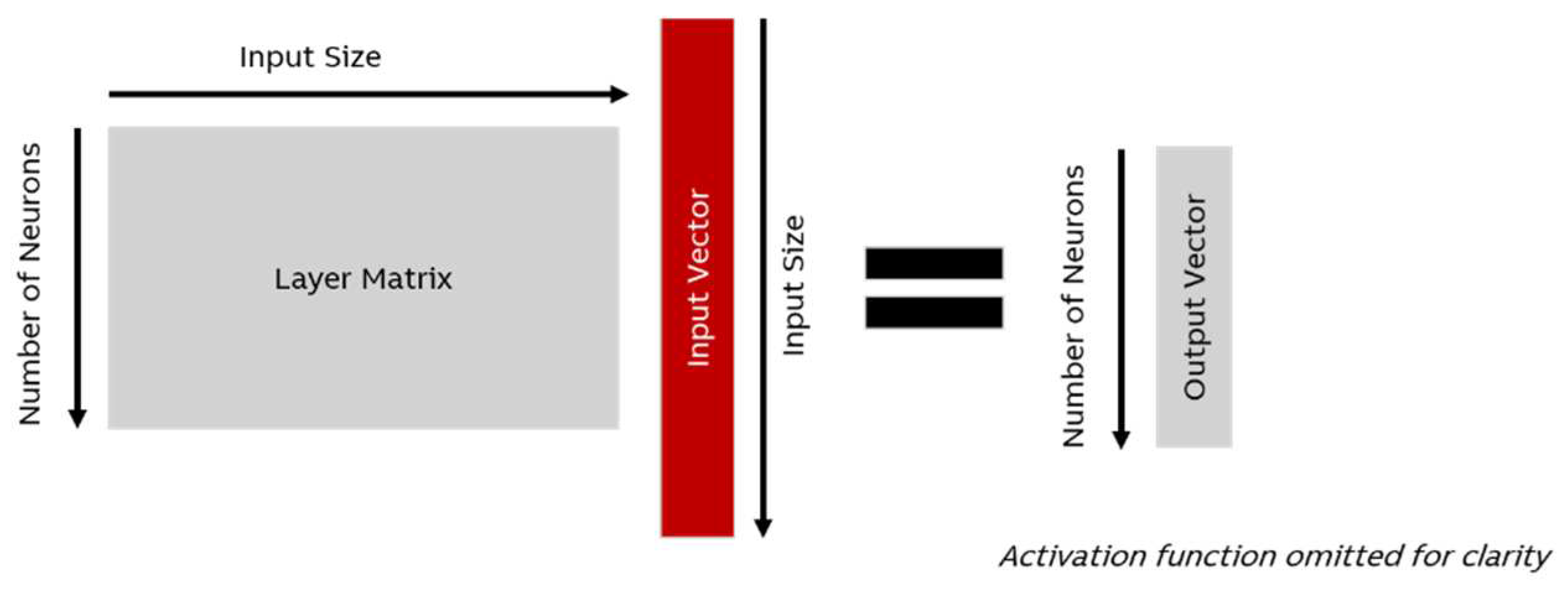
Other factors prevent the use of a simple formula. There are specialized layers (e.g., Convolutional Layers), that do not follow the pattern shown in
Figure 5 (cf. [
19]). Also, even for the basic operation shown in the figure, there are computational shortcuts that can be taken so the same model will have a different footprint on different hardware. The energy required for a single inference is best measured with a software tool instead of computed based on the hardware architecture, at least for a certain
kind of model and then used in the formula to understand the lifetime energy cost and to estimate training cost (see next section).
A good model architecture can achieve high performance with reduced energy consumption compared to a less efficient design (cf. [
22], [
11], [
29]). Patterson et al claim that an advanced architecture can reduce computation by factors of 5-10 [
8]. There are efficient architectures that consider the “
network complexity”, i.e., “
the interplay between accuracy, number of parameters, activations, and operations.” [
25]. Cai et al have studied various neural networks (CNNs in this case) and have found that for models of roughly the same performance, energy use varied by factor 40 [
22]. For example, Squeezenet is 1/50 the size of Alexnet with comparable performance [
35]. Generally, using smaller models is a good way to reduce the carbon footprint of AI [
36]. However, there can be a trade-off between performance and size reduction.
The naïve approach to getting small models is to limit oneself to low parameters counts from the beginning. On the other hand, there are several tools that help reduce the model size after training to reduce the energy cost at the inference stage. According to Patterson et al. “
pruning, quantization, and efficient coding” can improve a neural network’s energy efficiency by factor 3 to 7 [
6]. (For more details on pruning techniques see [
37].) Adding sparsity to models also reduces energy consumption which can be 10% of a dense model of the same size [
6]. Another way to reduce model size is knowledge distillation which trains a smaller model with random data classified by a larger model (cf. [
38]).
3.5. Training
While some authors propose to base training energy estimates on the training time and number of processors [
6], which is a reasonable approach, our consolidated model goes into more detail to better understand the factors that can be influenced. Based on ideas found in [
7] and [
17], the cost at this stage is proportional to three factors: The energy cost of a single inference (I), the size of the training data set (D) and the number of epochs (E). There is also significant overhead for the loss function and backpropagation step that is expressed as a factor
.
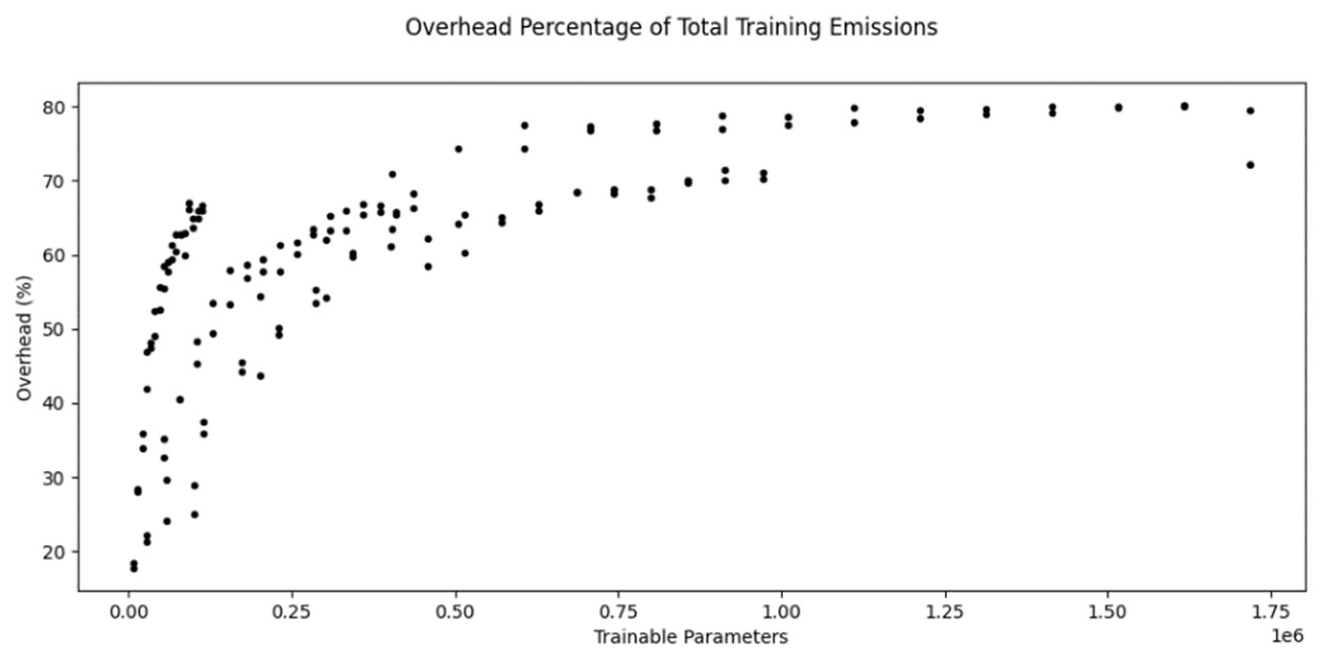
The formula implicitly takes into account the PUE and type of processor via I. However, it ignores static power consumption. Our experiments show that the overhead can be estimated to be 80% of the total training energy cost, i.e., the total training energy used is 5 times the energy used by the inferences on the training set alone for our setup (see section 0).
One way to reduce energy training cost suggested in the literature (cf. [
6], [
7], [
17], or [
39]) is transfer learning where a model trained on another data set is reused for a similar task [
40]. Transfer learning allows using a reduced data set and less epochs. In the example experiment conducted by Walsh et al, using a pretrained model was almost 15 times as energy efficient as training a model with the same architecture from scratch [
39]. Besides a reduced training time, the need to do model architecture search (see next section) is also resolved. However, our empirical analysis adds some caveats to this claim (Section 0).
3.6. Model Architecture Search
The development of ML code to solve a problem involves manual or automated testing of different model architectures to eventually meet the inference task’s requirements. The term for this activity is Model Architecture Search or Neural Architecture Search (NAS) in the case of neural networks [
6]. The process normally involves training the model to gain insights regarding the required architecture and using the best architecture in the end.
Based on ideas found in [
7], the cost at this stage (CT) is proportional to two factors: The cost of training and the number of times the hyperparameters are tuned (H). Some of T’s components, i.e., I, E, and D (see above), might vary for each tuning step resulting in different values of T for each step in the tuning.
Logically, each hyperparameter tuning loop requires the training of the model. The training in turn requires an inference for each entry in the data set and each epoch. So, if the energy needed for a single inference is known, the energy at the architecture search stage can at least be estimated.
The model does not consider the cost of activities such as data augmentation [
7] but unlike prior models takes into account training epochs and the fact that the full data set is not used at all steps (cf. [
6]).
The formulas above essentially states that smaller models (lower I) trained on less data (lower D) for a shorter time (lower E) are more energy efficient. Also, trying many different variants (H) multiplies the energy use, so good search strategies are important [
17].
On the other hand, increased model size, more data, longer training time, and better hyperparameter choices increase performance (albeit with diminishing returns [
7]). Also, a good architecture can be reused for a variety of related problems and can save a lot training energy for each problem. For example, the Meena NLP architecture is estimated to save an amount of energy that is 15 times larger than the energy cost that was needed to identify the architecture for every single additional case [
6].
The theoretical model implies a couple of measures to reduce the carbon footprint at this stage. In particular, anything that reduces the size of H is helpful. One suggestion is to avoid grid search (a common approach to testing hyperparameters) and use random search instead (see [
17]). Another option is to include other criteria than just accuracy in a NAS. A multi-criterion search including energy consumption can be used to produce more efficient models (cf. [
17] and [
19]).
3.7. Life Cycle Energy Use
Taking the three life cycle phases described above, the total life cycle energy use of the model can be computed in the following way:
where
CT is the energy cost of architecture search,
T the cost of the final training (if not part of
CT) and
I the cost of a single inference.
e is the expected number of inferences for the model. The use of even wider life cycle definitions is discussed in section 0.
3.8. Energy Use to Carbon Footprint Conversion
The conversion of energy use into Co
2eq is done by multiplying
EC, the energy cost of the activity under observation (inference, training, NAS, or life cycle), with the carbon emission factor (
EF) of the energy type consumed.
The importance of
EF should not be underestimated, because the CO
2eq emitted varies widely by geographical location. Location can influence this value by ~5X-10X, even within the same country and the same organization according to Patterson et al (see [
6] and [
8]); others say by factor 30 [
28], or even factor 40 according to [
17]. Optimizing location and time can reduce energy use by up to 80% according to Xu [
41]. Even in North America,
EF ranged from 20g CO
2eq/kWh in Quebec to 736.6g CO
2eq/kWh in Iowa in 2019 [
17]. This variation is due to the different energy mix, e.g., Quebec used 94% hydropower and Iowa used a lot of coal plants at that time. Therefore, choosing the right location “
is likely the easiest path for ML practitioners to reduce CO2eq” [
6]. On the other hand, renewable energy is not available in an unlimited amount, so saving energy is still the best way to avoid climate gas emissions even if more challenging.
3.9. Critical Examination of the Model and a Challenge to Its Assumptions
Obviously, the model above has a limited scope. It ignores a more complete life cycle that also includes the energy cost of producing and providing the hardware. As scope expands, so does the complexity of the estimation model. Even complex approaches from the prior art (such as [
28]) shy away from these aspects. The reason is that it is difficult to attribute manufacturing impacts to concrete ML experiments [
28]. If a university researcher uses a server to train and test a model but the server is also used by other researchers and for unknown tasks in the future, how much of its carbon footprint needs to be assigned to the current research activity? Logically, it cannot be all of it. A fraction makes sense, but the exact percentage of use is probably not known. However, a similar problem was faced by classical manufacturing cost calculation. The solution there was Activity Based Costing (ABC) [
42], which uses specific methods to assign the cost of overhead activities to actual product units with the goal of helping understand the correct cost impact of each item. Similar techniques could be used for carbon accounting.
Inference cost is not detailed in our model even though the basic mathematical operations of machine learning are well known, and the exact number of operations can be determined analytically (cf. [
25]). While some authors consider the use of floating point operations (FPOs/FLOPs) to be a good driver for energy use ( [
7] or as at least a proxy value by [
43] and [
25]), several authors have criticized this metric (cf. [
22], [
28], and [
25]; also see [
19]). They have shown empirically that there is not a strong correlation between FPOs and energy consumption unless the architectures are relatively close, i.e., they use the same kinds of operations but in different numbers ( [
28], also see [
22]). Software to measure FPOs exists, e.g., swall0w
7 and
torchstat8.
4. Empirical Evaluation and Carbon Footprints of Different Models
The theoretical model described above is an amalgamation of theoretical models and metrics found in the literature. In this section, we show the results of some experiments intended to give some indication of the correctness of these ideas. Our intention is to confirm or challenge the various claims in the literature. We believe that multiple authors need to conduct such experiments to advance the understanding in this regard, so we replicate some experiments found in the literature as well.
We look at the different parameters used above to study their impact. In particular, we examine key aspects of the model architecture, the training set size, and the number of epochs. Due to cost constraints, we did not test different hardware architectures. The code was tested on a test machine with specs as summarized in
Table 2. For emission calculations, the energy mix of Germany was assumed. Most of the models used were “dummy models” that were not optimized for accuracy or any particular task. Rather they were chosen for their shape, depth, and layer types. While this might be a limitation, it allowed specifically testing different model sizes and shapes within our time budget.
The experiments confirm that training set size and the number of epochs drive the energy cost (0 and 0). There are some indicators that pretrained models could help reduce carbon footprint during training but the example found in the literature might be ill-chosen (0). Another experiment helps us understand the overhead due to backpropagation and loss function calculation during training (see 0). Finally, the general consensus that model size influences energy use but is not a clear-cut indicator due to other factors has been confirmed by our experiments (0).
4.1. Training Set Size
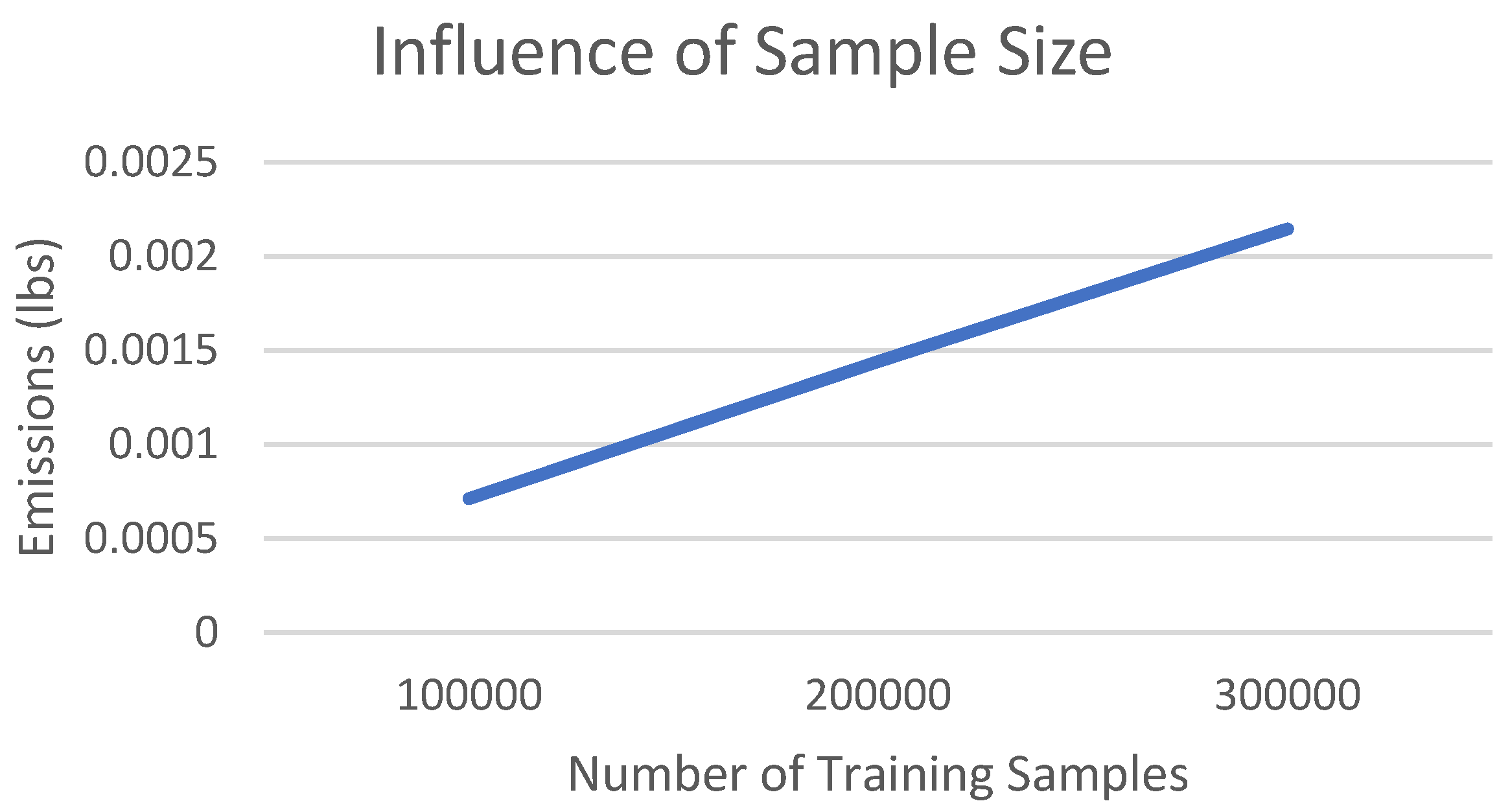
As described in section 0, the energy cost of training is driven by the cost of a single inference, the size of the training set, and the number of training epochs. In practice, more training data is one recipe to improve model performance. In a simple experiment conducted by us, increasing the sample size linearly increased the energy use (which is in line with what one would expect.) The results are shown in
Figure 6.
4.2. Number of Training Epochs
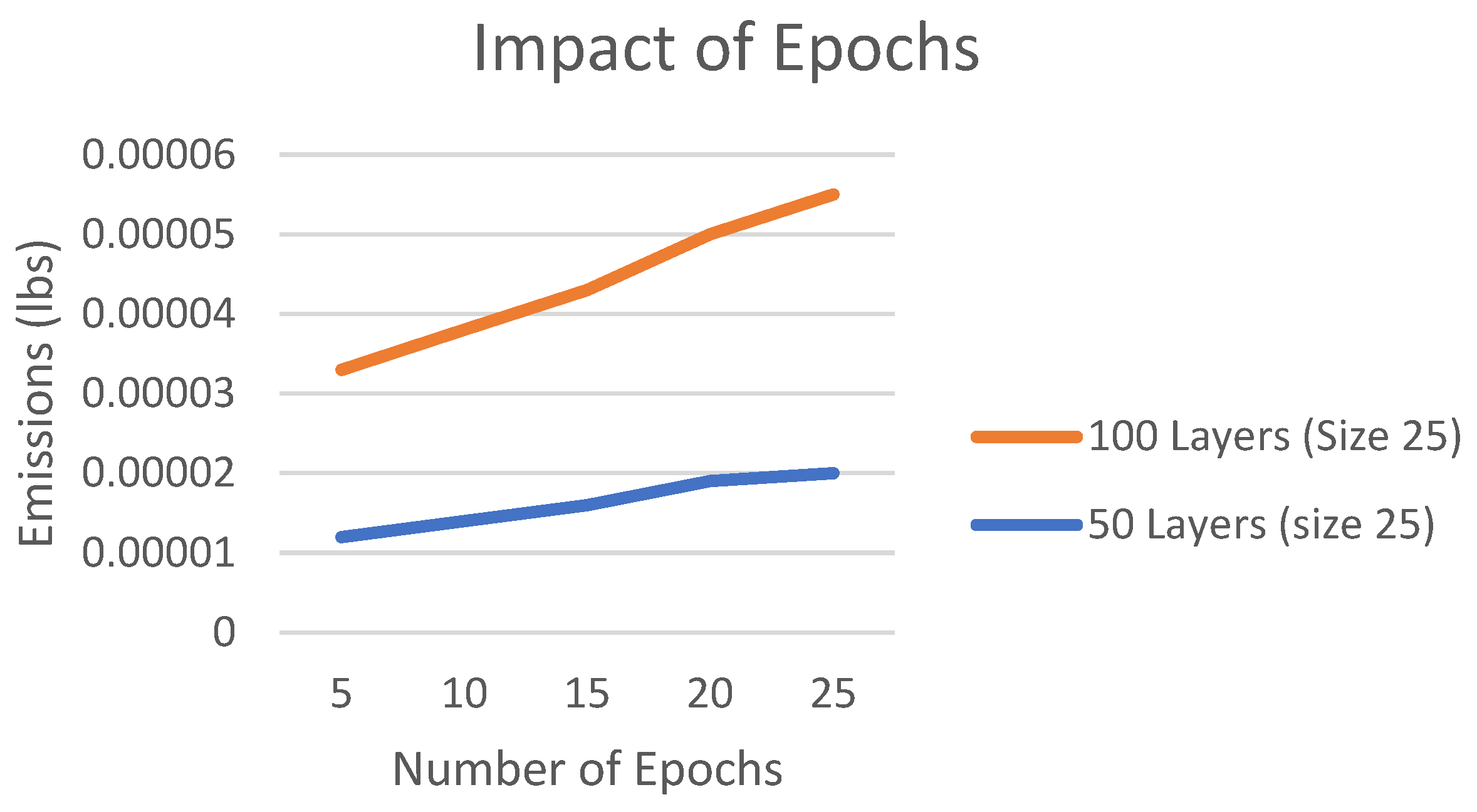
Similarly, the longer you train a model (i.e., more epochs) the more energy you use. Again, this increase is expected to be mostly linear.
Figure 7 shows experimental results for 2 different models.
4.3. Transfer Learning and Pretrained Models
Using pre-trained models is frequently mentioned in the literature as a possible way to save energy during the training phase (cf. [
6], [
7], [
17], [
39]). In the example experiment conducted by Walsh et al, using a pretrained model was almost 15 times as energy efficient as training a model with the same architecture from scratch. The example used was the Xception model repurposed for classification on the “cats vs dogs” data set [
39]. The energy consumption is shown in
Table 3. RCvD is a case where the Xception model architecture was trained from scratch to classify cats and dogs. TLCvD is the transfer learning experiment from the paper, TLRep is our replication of the TLCvD experiment
9.
However, it should be noted that Xception is already capable of distinguishing dogs and cats (even different breeds)
10 so critical readers might consider this example to be artificial. Thus, for further analysis, we have performed transfer learning with Xception for MNIST classification
11 with 6 epochs (TLMNIST). Training Xception from scratch with MNIST yields poor results with no real improvement even after 20 epochs (RMNIST). A dedicated model
12 (DMNIST) on the other hand does yield better results with less energy use.
In our view, these experiments have certain implications on the benefits of transfer learning. It is true, that a model of the same complexity can be attained with less energy. However, if the problem is of lesser complexity, a dedicated model can be designed that uses even less energy than transfer learning. In the case of MNIST and Xception, defaulting to a pretrained model leads to an increase in energy consumption by factor 90 over the dedicated model. The main benefit of pretrained models seems to be that they save the developer a lot of time during the model architecture search phase and not necessarily energy savings.
4.4. Training vs Inference
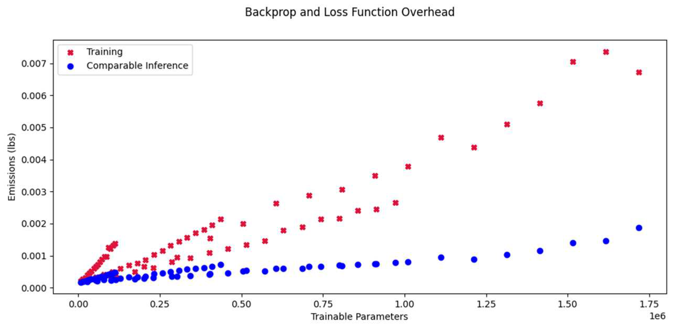
The overhead caused by back propagation, the calculation of the loss function and these things during training is hard to quantify analytically. In this experiment we compare running inferences on the training data set (size 100’000) and doing actual training (which is inference plus overhead). We have examined several networks of different depths and different uniform layer sizes (see
Table 4).
The resulting emissions are shown in
Figure 8. Clearly, the overhead is no fixed offset.
When expressed as a percentage of the total training emissions, the overhead appears to asymptotically approach a value of about 80%.
Figure 9 shows this overhead for the experiments from above as well as the same models trained with 10000 samples.
4.5. Impact of Model Architecture
There is a general consensus that models use more energy for inference as they grow in size. However, it is not easy to map size-related model properties to energy consumption. Also, the shape of the model and the type of layer used seem to play a role. We have conducted a series of experiments with different models to see the impact of these parameters.
4.5.1. Impact of Model Size
While the connection between model size and energy use is not straightforward, larger models
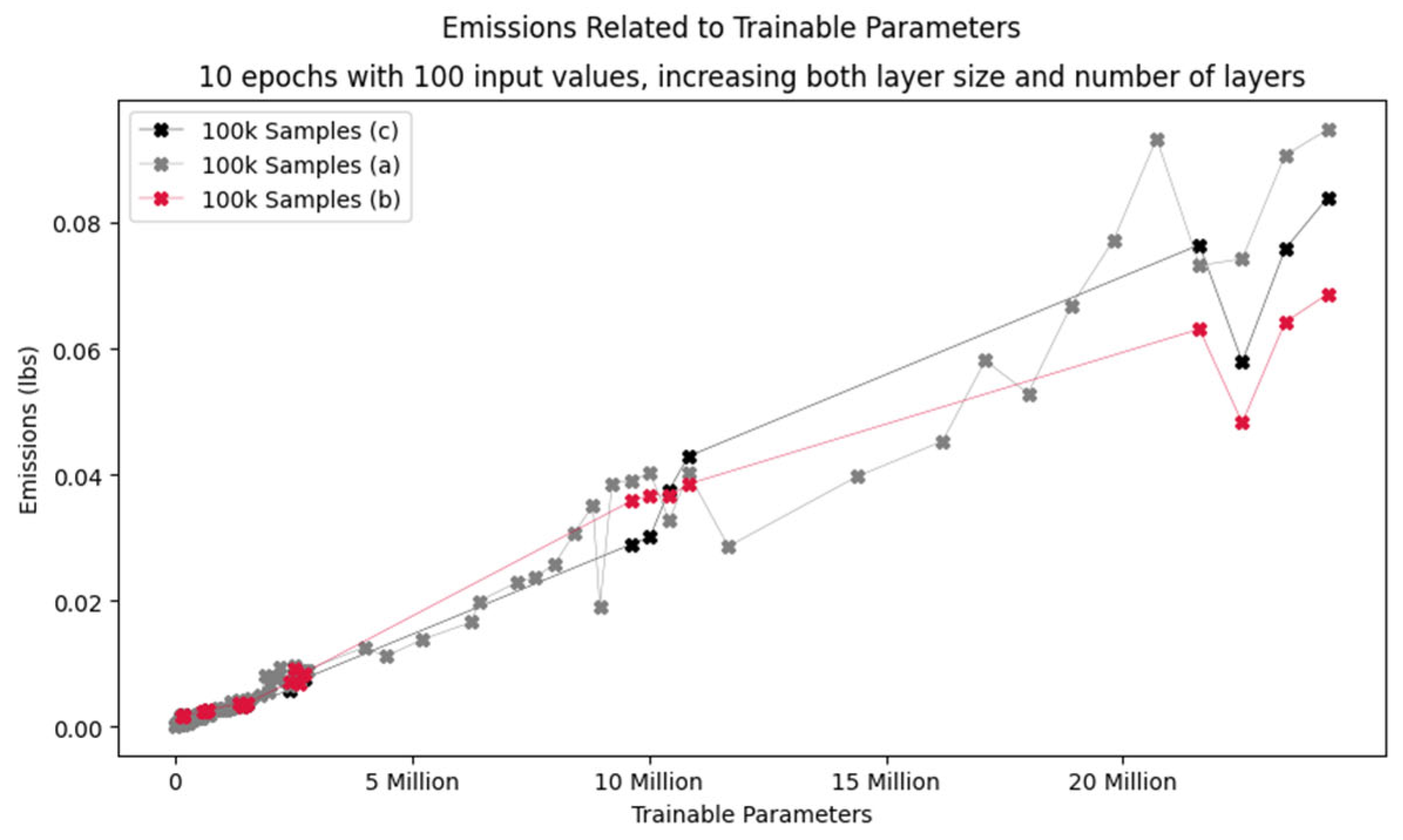
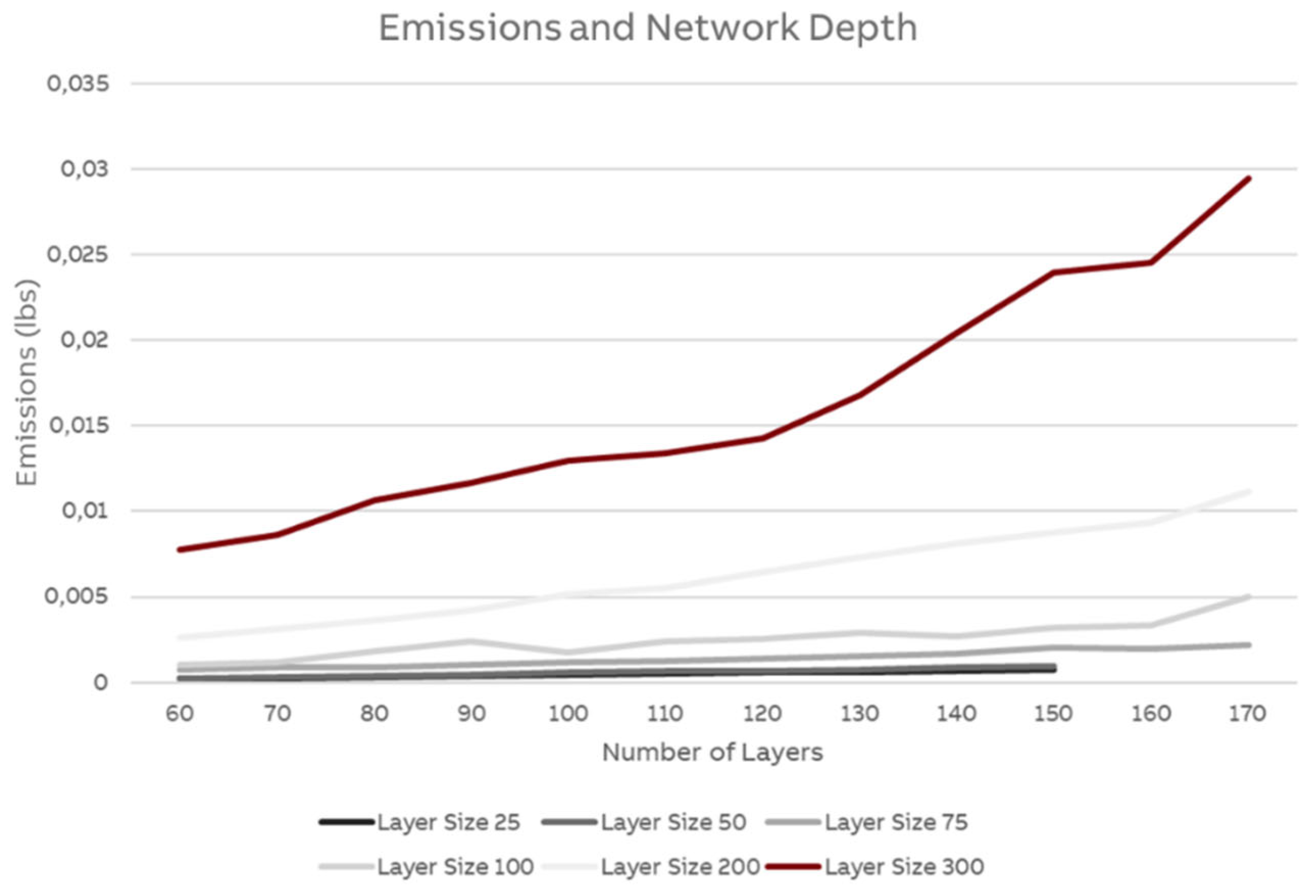
generally need more energy than smaller models, especially if the model properties are mostly the same otherwise. We have run a series of experiments to determine the overall impact of size. In the experiments, layer size varied between 25 and 100 nodes and the number of layers ranged from 10 to 170. The models were trained for 10 epochs with 100’000 samples. The results can be seen in
Figure 10. While there are some jumps, the general trend is that as model size increases, so does energy use. (For some possible explanations for the jumps, see section 0)
A more detailed analysis of network growth for different layer sizes is shown in
Figure 11.
4.5.2. Impact of Model Shape
While model size has an impact on energy use, the number of trainable parameters is only of limited use for estimating the energy footprint [
19]. One of the reasons for this phenomenon is the influence of the model shape. Lai et al have shown that models of the same “family” that have different layer sizes, depths, and layer types but the same ops count and accuracy can vary in energy use by up to 30% [
19]. Other authors mention a factor of 5 [
19]. As shown in
Table 5, models with the same node count can have vastly different trainable parameter counts.
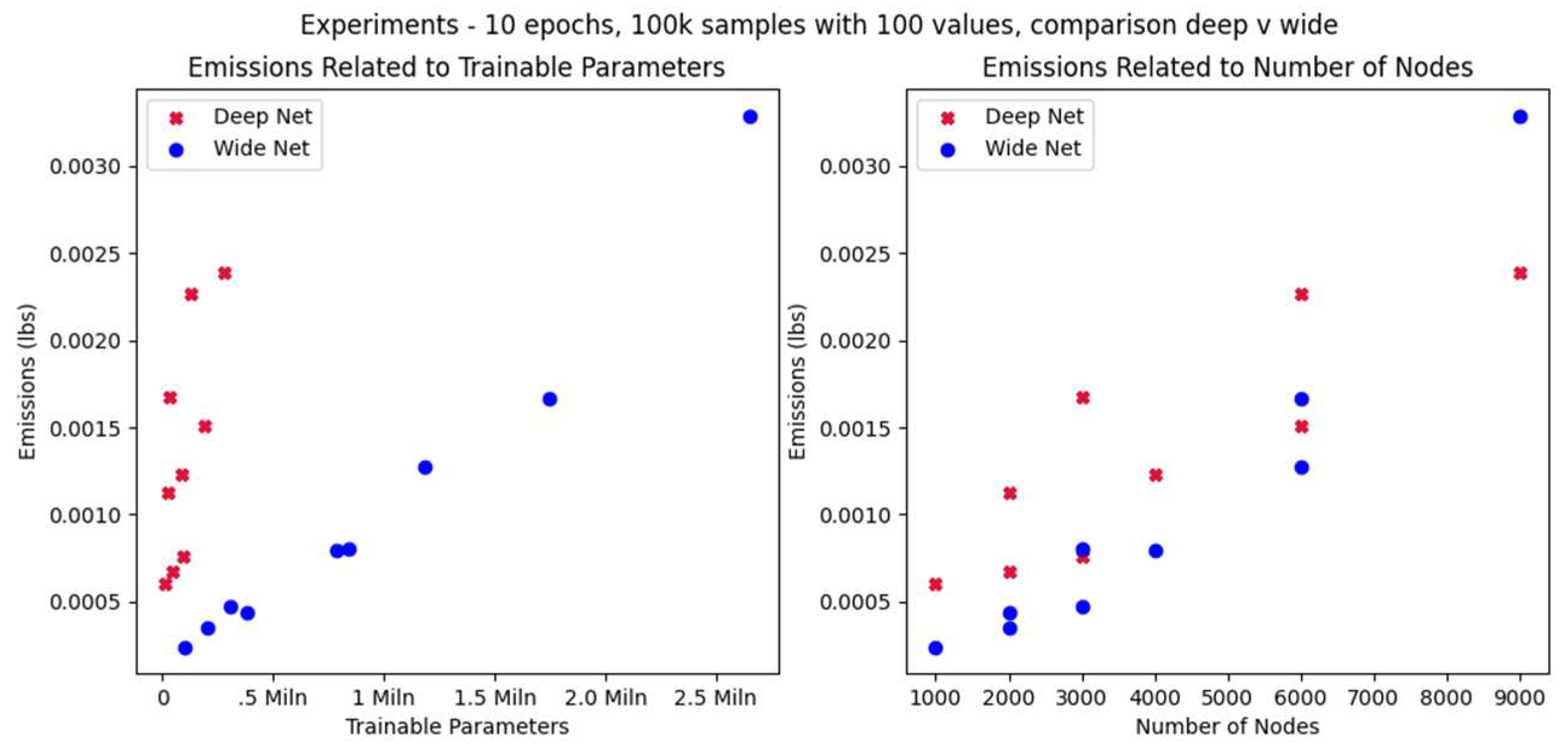
With regard to carbon footprint, wide models (few layers with many nodes) be-have differently from deep models (many relatively small layers). We ran a series of experiments with the results shown in
Table 6 and
Figure 12.
The energy use of deep networks increases a lot faster than that of wide networks of the same number of trainable parameters (
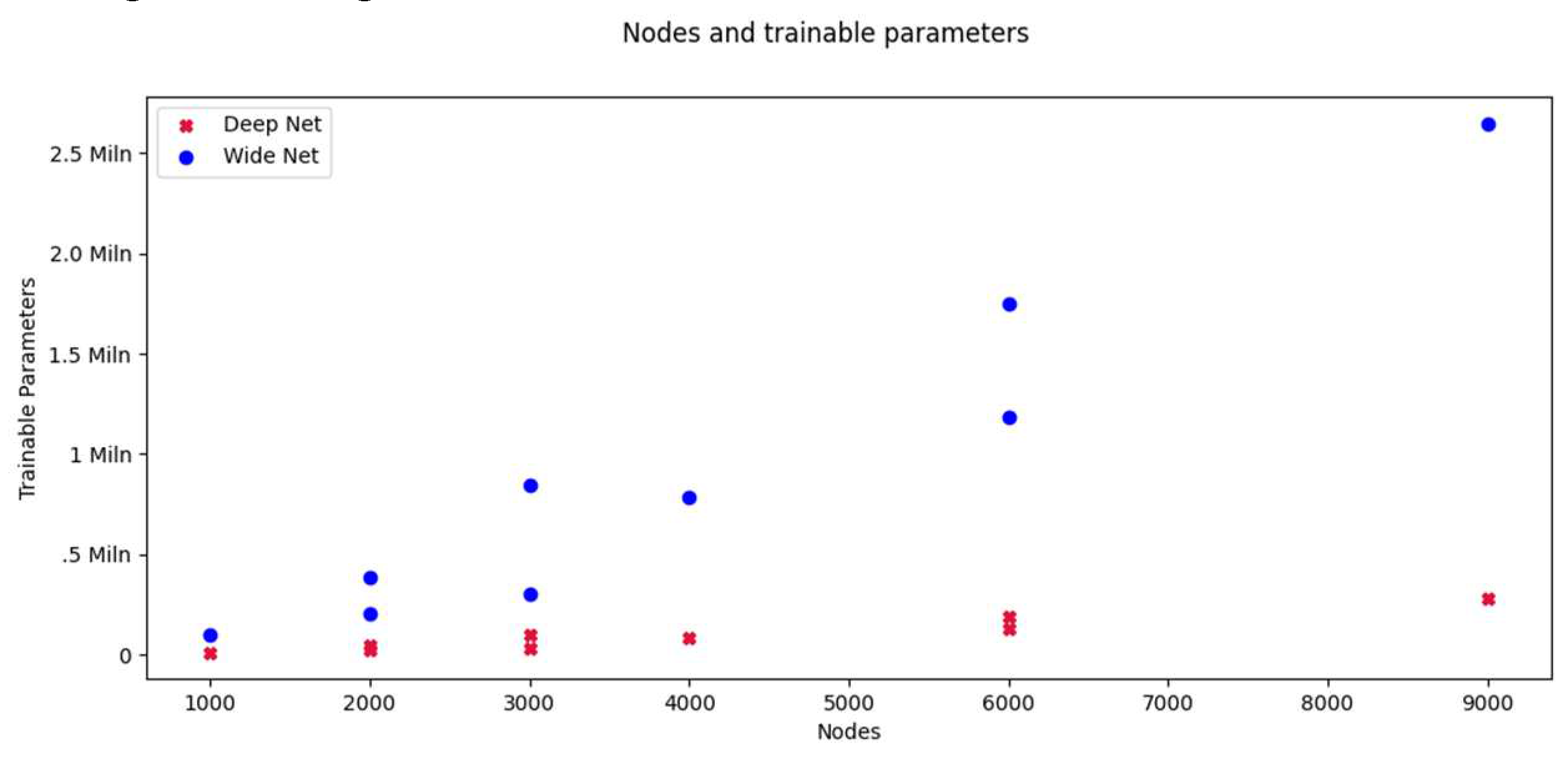
Figure 12, left). On the other hand, a deep model with the same number of nodes as a wide model will have significantly less trainable parameters (
Figure 13), one of the facts used by SqueezeNet to reduce its size [
25]. Thus, a deep model with the same number of nodes as a wide model will need more energy and will have less trainable parameters. It is obvious that trainable parameters are not a good metric to compare models of different shapes. The same applies to the number of nodes (
Figure 12, right).
However, one cannot automatically draw the conclusion that wide networks are preferable to deep ones. In fact, Zhou et al have shown that depth is better at increasing expressive power of a neural network [
44].
4.5.3. Impact of Layer Type
Certain papers (e.g. [
20] or [
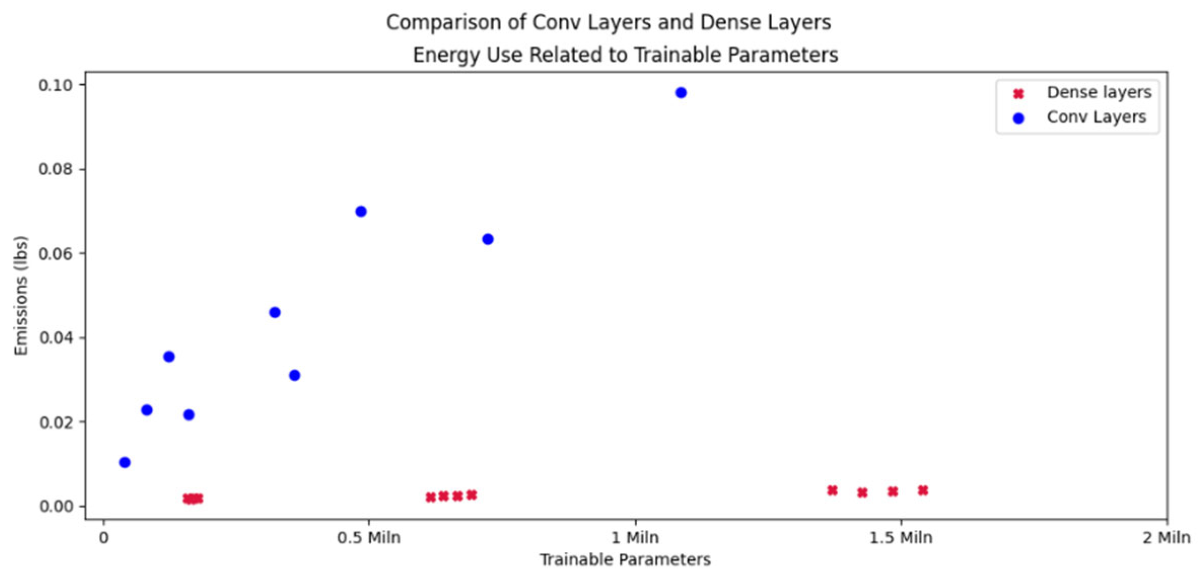
22]) stress the different behavior of specific layer types such as convolutional layers. To get a rough impression of the impact of layer type, two groups of models where compared. One is a series of wide dense models (see
Figure 12), the other is a series of similarly-shaped convolutional layers (where the “width” is represented by the number of filters).
Figure 14 compares the models by trainable parameters. As can be seen, purely convolutional models with the same number of trainable parameters consume a lot more energy.
5. Conclusions
In this paper, we have studied theoretical models and empirical studies to predict the carbon footprint of a machine learning model. We ran our own experiments to test some of the statements in the literature. Based on this, we can draw the following conclusions.
Consolidated model: We created a consolidated model that describes the factors that influence the carbon footprint at each life cycle stage of a machine learning model. This model helps understanding the benefit of various rule of thumbs to reduce carbon footprint (e.g., transfer learning or model distillation). However, it is not suitable for an exact prediction. The experiments have confirmed that there are no simple metrics and formulas that work correctly.
Experimental confirmation of literature: Many of the statements found in the literature could be confirmed by our experiments. Epochs and training set size are of vital importance. Trainable parameters are a basic indicator but only if comparing models that share many properties such as general shape and type of layers. However, we find that the arguments for transfer learning can be challenged and need further investigation.
Carbon footprint is a problem but often not a huge problem: While there are high-end models that use a lot of energy during architecture search and training, the typical use case will not have a significant impact in that regard. If the model is successful and sees a lot of use, the inference phase is more important than the initial phases. Thus, it would seem to be a good practice to optimize the inference stage once a good model is achieved. Since a single inference is not very expensive, tests can be run to understand the cost and to test reduction methods. Nevertheless, even though most models are not a problem at the moment, any concept that relies on an increasing carbon footprint for improvement (“red AI” [7]) needs close monitoring and corrective steps.
More work is needed if one sees the need for a model that is actually capable to predict ML carbon footprint ex ante. One step into that direction are more experiments to understand the various details, which is future work we plan to address in our next papers.
Notes
| 1 |
|
| 2 |
|
| 3 |
|
| 4 |
|
| 5 |
|
| 6 |
Technically, nnU-Net is more than just model training, it includes a hyperparameter search. |
| 7 |
Swall0w (Swall0w) · GitHub |
| 8 |
|
| 9 |
|
| 10 |
|
| 11 |
Slightly adapting the cats_v_dogs code used for the TLR experiment |
| 12 |
|
References
- D. Crouse, H. Han, D. Chandra, B. Barbello and A. K. Jain, "Continuous authentication of mobile user: Fusion of face image and inertial Measurement Unit data," in International Conference on Biometrics (ICB), 2015.
- T. Brown, B. Mann, N. Ryder, M. Subbiah, J. Kaplan, P. Dhariwal, A. Neelakantan, P. Shyam, G. Sastry, A. Askell and S. Agarwal, "Language models are few-shot learners," Advances in neural information processing systems, vol. 33, pp. 1877-1901, 2020.
- R. Gitzel, H. Kaul and M. Dix, "Maps of Infrared Images to Detect Equipment Faults," in IEEE Eighth International Conference on Big Data Computing Service and Applications, 2022.
- M. Gärtler, V. Khaydarov, B. Klöpper and L. Urbas, "The Machine Learning Life Cycle in Chemical Operations – Status and Open Challenges," Chemie Ingenieur Technik, vol. 93, no. 12, pp. 2063-2080, 2021. [CrossRef]
- O. Y. Al-Jarrah, P. D. Yoo, S. Muhaidat, G. K. Karagiannidis and K. Taha, "Efficient Machine Learning for Big Data: A Review.," Big Data Research 2 (3), p. 87–93, 2015. [CrossRef]
- D. Patterson, J. Gonzalez, Q. Le, C. Liang, L.-M. Munguia and D. e. a. Rothchild, "Carbon emissions and large neural network training.," in In arXiv preprint. arXiv:2104.10350., 2021.
- R. Schwartz, J. Dodge, N. A. Smith and O. Etzioni, " Green AI," Commun. ACM 63 (12), p. 54–63, 2020.
- D. Patterson, J. Gonzalez, U. Hölzle, Q. Le, C. Liang, L.-M. Munguia, D. Rothchild, D. R. So, M. Texier and J. Dean, "The Carbon Footprint of Machine Learning Training Will Plateau, Then Shrink," IEEE Computer, vol. 55, no. 7, pp. 18-28, 2022.
- E. García-Martín, C. F. Rodrigues, G. Riley and H. Grahn, "Estimation of energy consumption in machine learning.," Journal of Parallel and Distributed Computing 134, p. 75–88, 2019.
- A. Gupta, "The current state of affairs and a roadmap for effective carbon-accounting tooling in AI," 2021. [Online]. Available: https://devblogs.microsoft.com/sustainable-software/the-current-state-of-affairs-and-a-roadmap-for-effective-carbon-accounting-tooling-in-ai/?WT.mc_id=green-30456-cxa. [Accessed 17 08 2022].
- K. Lottick, S. Susai, S. A. Friedler and J. P. Wilson, "Energy Usage Reports: Environmental awareness as part of algorithmic accountability," arXiv, 2019.
- G. S. F. S. W. Group, "Software Carbon Intensity (SCI) Standard," Greensoftware.foundation, 2021. [Online]. Available: https://github.com/green-software-foundation/software_carbon_intensity/. [Accessed 7 10 2022].
- D. Brooks, V. Tiwari and M. Martonosi, "Wattch: A framework for architectural-level power analysis and optimizations," ACM SIGARCH Computer Architecture News, vol. 28, no. 2, p. 83–94, 2000.
- C. Blakeney, "MARCHER: A Fine Grained Software Energy Efficiency Measuring Platform," 2021. [Online]. Available: https://greensoftware.foundation/articles/marcher-the-need-for-a-fine-grained-software-energy-efficiency-measuring-platform. [Accessed 7 10 2022].
- F. D. H., "Recent Advances in AI for Computational Sustainability," IEEE Intelligent Systems, vol. 31, no. 4, p. 56–61, 2016.
- T. Ahmad, D. Zhang, C. Huang, H. Zhang, N. Dai, Y. Song and H. Chen, "Artificial intelligence in sustainable energy industry: Status Quo, challenges and opportunities," Journal of Cleaner Production, vol. 289, 2021.
- A. Lacoste, A. Luccioni, V. Schmidt and T. Dandres, "Quantifying the Carbon Emissions of Machine Learning: arXiv, 2019. [CrossRef]
- E. Strubell, A. Ganesh and A. McCallum, "Energy and Policy Considerations for Deep Learning," in NLP: arXiv, 2019. [CrossRef]
- L. Lai, N. Suda and V. Chandra, "Not All Ops Are Created Equal!," in SysML Conference, Stanford, CA, USA, 2018.
- T.-J. Yang, Y.-H. Chen, J. Emer and V. Sze, "A method to estimate the energy consumption of deep neural networks," in 20th IEEE/ACM International Symposium on Cluster, Cloud and Internet Computing (CCGRID), 2020.
- A. Gupta, "Beyond Single-Dimensional Metrics for Digital Sustainability," [Online]. Available: https://greensoftware.foundation/articles/beyond-single-dimensional-metrics-for-digital-sustainability. [Accessed 10 07 2022].
- E. Cai, D.-C. Juan, D. Stamoulis and D. Marculescu, "NeuralPower: Predict and Deploy Energy-Efficient Convolutional Neural Networks," in PMLR (Proceedings of Machine Learning Research, 77), Seoul, Korea, 2017.
- W. Yuxin, W. Qiang, S. Shaohuai, H. Xin, T. Zhenheng, Z. Kaiyong and C. Xiaowen, "Benchmarking the performance and energy efficiency of AI accelerators for AI training," in 20th IEEE/ACM International Symposium on Cluster, Cloud and Internet Computing (CCGRID). IEEE, 2020., 2020.
- R. Selvan, N. Bhagwat, L. F. W. Anthony, B. Kanding and E. B. Dam, "Carbon Footprint of Selecting and Training Deep Learning Models for Medical Image Analysis," arXiv preprint. arXiv:2203.02202, 2022.
- L. Heim, A. Biri, Z. Qu and L. Thiele, " Measuring what Really Matters: Optimizing Neural Networks for TinyML," arXiv, 2021.
- G. Abhishek, "What do we need to build more sustainable AI systems?," 2021. [Online]. Available: https://greensoftware.foundation/articles/what-do-we-need-to-build-more-sustainable-ai-systems. [Accessed 17 08 2022].
- L. Lannelongue, J. Grealey and M. Inouye, "Green Algorithms: Quantifying the carbon footprint of computation," arXiv, 2020.
- P. Henderson, J. P. Henderson, J. Hu, J. Romof, E. Brunskill, D. Jurafsky and J. Pineau, "Towards the Systematic Reporting of the Energy and Carbon Footprints of Machine Learning.," Journal of Machine Learning Research, p. 1–43, 2020.
- X. Z. L. L. Y. W. a. W. S. Mohit Kumar, "Energy-Efficient Machine Learning on the Edges," in IEEE International Parallel and Distributed Processing Symposium Workshops (IPDPSW), 2020.
- T. Trader, "AWS to Offer Nvidia's T4 GPUs for AI Inferencing," 2019. [Online]. Available: https://www.hpcwire.com/2019/03/19/aws-upgrades-its-gpu-backed-ai-inference-platform/. [Accessed 17 08 2022].
- J. Barr, "Amazon EC2 Update – Inf1 Instances with AWS Inferentia Chips for High Performance Cost-Effective Inferencing," 2019. [Online]. Available: https://aws.amazon.com/blogs/aws/amazon-ec2-update-inf1-instances-with-aws-inferentia-chips-for-high-performance-cost-effective-inferencing/. [Accessed 17 08 2022].
- M. Horowitz, "1.1 Computing's energy problem (and what we can do about it)," 2014 IEEE International Solid-State Circuits Conference Digest of Technical Papers (ISSCC), pp. 10-14, 2014.
- E. Jaureguialzo, "PUE: The Green Grid metric for evaluating the energy efficiency in DC (Data Center). Measurement method using the power demand," in IEEE 33rd International Telecommunications Energy Conference (INTELEC), 2011.
- A. Lawrence, "Data center PUEs flat since 2013," 2020. [Online]. Available: https://journal.uptimeinstitute.com/data-center-pues-flat-since-2013/. [Accessed 17 08 2022].
- F. N. S. H. M. W. M. K. A. W. J. D. a. K. K. Iandola, "SqueezeNet: AlexNet-level accuracy with 50x fewer parameters and<0.5 MB model size," arXiv.
- A. Gupta, "Why should sustainability be a first-class consideration for AI systems?," 2021. [Online]. Available: https://greensoftware.foundation/articles/why-should-sustainability-be-a-first-class-consideration-for-ai-systems. [Accessed 17 08 2022].
- D. J. J. G. O. J. F. a. J. G. Blalock, " What is the state of neural network pruning?," in Proceedings of machine learning and systems 2, 2020.
- G. Hinton, O. Vinyals and J. Dean, "Distilling the Knowledge in a Neural Network," arXiv, 2015.
- W. Paul, B. Jhilam, S. V. Saujanya, K. Vikrant, R. R. M and R. O. (Eds.), Sustainable AI in the Cloud: Exploring Machine Learning Energy Use in the Cloud. 2021. [CrossRef]
- L. Torrey and J. Shavlik, "Transfer learning," in Handbook of research on machine learning applications and trends: algorithms, methods, and techniques, IGI global, 2010, p. 242–264.
- T. Xu, "These simple changes can make AI research much more energy efficient ( MIT Technology Review)," 2022. [Online]. Available: https://www.technologyreview.com/2022/07/06/1055458/ai-research-emissions-energy-efficient/?truid=&utm_source=the_download&utm_medium=e. [Accessed 17 08 2022].
- R. S. Kaplan and W. Bruns, Accounting and Management: A Field Study Perspective, Harvard Business School Press, 1987.
- L. Heim, A. Biri, Z. Qu and L. Thiele, "Measuring what Really Matters: Optimizing Neural Networks for TinyML," arXiv, 2021.
- Z. Lu, H. Pu, F. Wang, Z. Hu and L. Wang, "The expressive power of neural networks: A view from the width," in NIPS, 2017.
- C. Blakeney, "MARCHER: A Fine Grained Software Eenergy Efficiency Measuring Platform," 2021. [Online]. Available: https://greensoftware.foundation/articles/marcher-the-need-for-a-fine-grained-software-energy-efficiency-measuring-platform. [Accessed 17 08 2022].
- S. A., J. P. L. K. Wilson, S. Susai and Friedler, "Energy Usage Reports: Environmental awareness as part of algorithmic accountability," arXiv, 2019.
- S. A. E. E. C. N. N. f. Mobile, "ShuffleNet: An Extremely Efficient Convolutional Neural Network for Mobile," in IEEE/CVF Conference on Computer Vision and Pattern Recognition, 2018.
|
Disclaimer/Publisher’s Note: The statements, opinions and data contained in all publications are solely those of the individual author(s) and contributor(s) and not of MDPI and/or the editor(s). MDPI and/or the editor(s) disclaim responsibility for any injury to people or property resulting from any ideas, methods, instructions or products referred to in the content. |
© 2023 by the authors. Licensee MDPI, Basel, Switzerland. This article is an open access article distributed under the terms and conditions of the Creative Commons Attribution (CC BY) license (http://creativecommons.org/licenses/by/4.0/).
