Preprint

Article

Trainable Activations for Image Classification

Altmetrics

Downloads

2614

Views

1128

Comments

Evgenii Pishchik^*

This version is not peer-reviewed

This preprints belongs to the Topic

Computer Vision and Image Processing

Submitted:

22 January 2023

Posted:

26 January 2023

You are already at the latest version

Alerts

Abstract

Non-linear activation functions are one of the main parts of deep neural network architectures. The choice of the activation function can affect model speed, performance and convergence. Most popular activation functions don't have any trainable parameters and don't alter during the training. We propose different activation functions with and without trainable parameters. Said activation functions have a number of advantages and disadvantages. We'll be testing the performance of said activation functions and comparing the results with widely known activation function ReLU. We assume that the activation functions with trainable parameters can outperform functions without ones, because the trainable parameters allow the model to "select'' the type of each of the activation functions itself, however, this strongly depends on the architecture of the deep neural network and the activation function itself.

Keywords:

Subject: Computer Science and Mathematics - Computer Vision and Graphics

1. Introduction

As deep neural networks developed, various activation functions were used and non-linearity remained the main requirement for all functions, which allows you to build deeper neural networks operating in more complex domains.

Sigmoid was one of the first successful activation functions. It performed well in simple tasks, but was not suitable for more complex tasks due to the problem of vanishing gradient [2]. The Rectified Linear Unit (ReLU) has become extremely popular in deep neural networks, getting rid of the problem of the vanishing gradient that Sigmoid had. However, ReLU has its own problems too, for example shifted from zero mean unit. Leaky ReLU [3], Exponential Linear Unit (ELU) [4] activation functions were designed to get rid of hard nullifying in the negative area, as well as to shift the mean unit closer to zero.

Most of these activation functions are non-trainable. We have developed several trainable activation functions to expand this set, with some of them showing better performance than non-trainable ones under certain conditions, which we will talk about later.

The article is structured as follows: In Section 2, we discuss the related works. In Section 3, we discuss the proposed approach. Section 4 contains the presentation of the results. We end with concluding remarks in Section 5.

2. Related Work

We have found several major articles that propose the trainable activation functions.

Sinu-Sigmoidal Linear Unit (SinLU) [5] is an activation function that has two trainable parameters, first one is the amplitude of the sine function, second one is the frequency of the sine wave. The main property of this function is the usage of periodical properties of the sine function.

ErfAct and Pserf [9] are trainable activation functions that are based on the Gauss error function and can be interpreted as smooth approximations of the ReLU. These functions outperform the ReLU and some other standard activation functions, but are more computationally non efficient. Forward pass of these functions is almost 1.5 times slower than that of the ReLU and the backward pass is 2 times slower.

Fourier-CNN and LC-CNN [10] are convolutional neural networks that use fourier series and linear combination as their activation functions.

In [11] authors review a large set of trainable activation functions and conduct a comparison using different datasets and model architectures. Authors divided them into two major categories: parameterized standard functions and functions based on ensemble methods. Parameterized standard functions are modifications of the standard activation functions using trainable parameters. Functions based on ensemble methods are combinations of different functions using trainable parameters.

Given articles inspired us to conduct this study: to create our own trainable activation functions and to modify existing ones so that they can compete with and, possibly, outperform current most popular choice when it comes to activation functions.

3. Proposed Approach

In this section, we discuss the proposed activation functions — Cosinu-Sigmoidal Linear Unit (CosLU), DELU, Linear Combination (LinComb), Normalized Linear Combination (NormLinComb), Rectified Linear Unit N (ReLUN), Scaled Soft Sign (ScaledSoftSign), Shifted Rectified Linear Unit (ShiLU). Each of these functions has its own advantages and disadvantages, some of them suffer from ReLU problems (ReLUN, ShiLU) because they were designed as ReLU modification, some may suffer from the problem of a vanishing gradient (ScaledSoftSign), some lose in the model speed (LinComb and NormLinComb).

3.1. CosLU

In this section, we discuss the proposed activation function, which is defined by Equation 1.

C o s L U (x) = (x + α cos (β x)) σ (x)

(1)

Here

σ

is a sigmoid function (Equation 2) and

α

and

β

are trainable parameters.

σ (x) = \frac{1}{1 + e^{- x}}

(2)

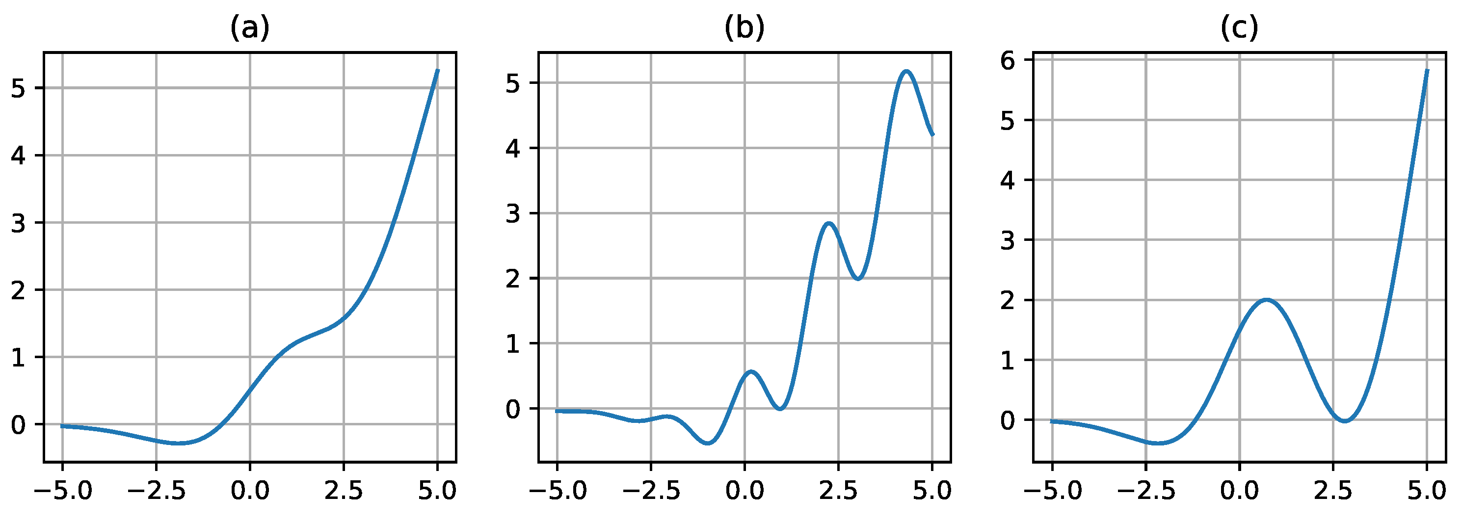
Proposed function is similar to SinLU but uses a different type of periodic function, a cosine function is used instead of a sine function. Parameter

α

controls the cosine amplitude, thereby determining the effect of the cosine on the entire activation function, parameter

β

controls the cosine frequency. Figure 1 shows different variants of the CosLU activation function with different values of parameters

α

and

β

3.2. DELU

In this section, we discuss the proposed activation function, which is defined by Equation 3.

D E L U (x) = \{\begin{matrix} S i L U (x), x ⩽ 0 \\ (n + 0.5) x + | e^{- x} - 1 |, x > 0 \end{matrix}

(3)

Here SiLU is Sigmoid Linear Unit (SiLU) [6] activation function and n is a trainable parameter.

S i L U (x) = x σ (x)

(4)

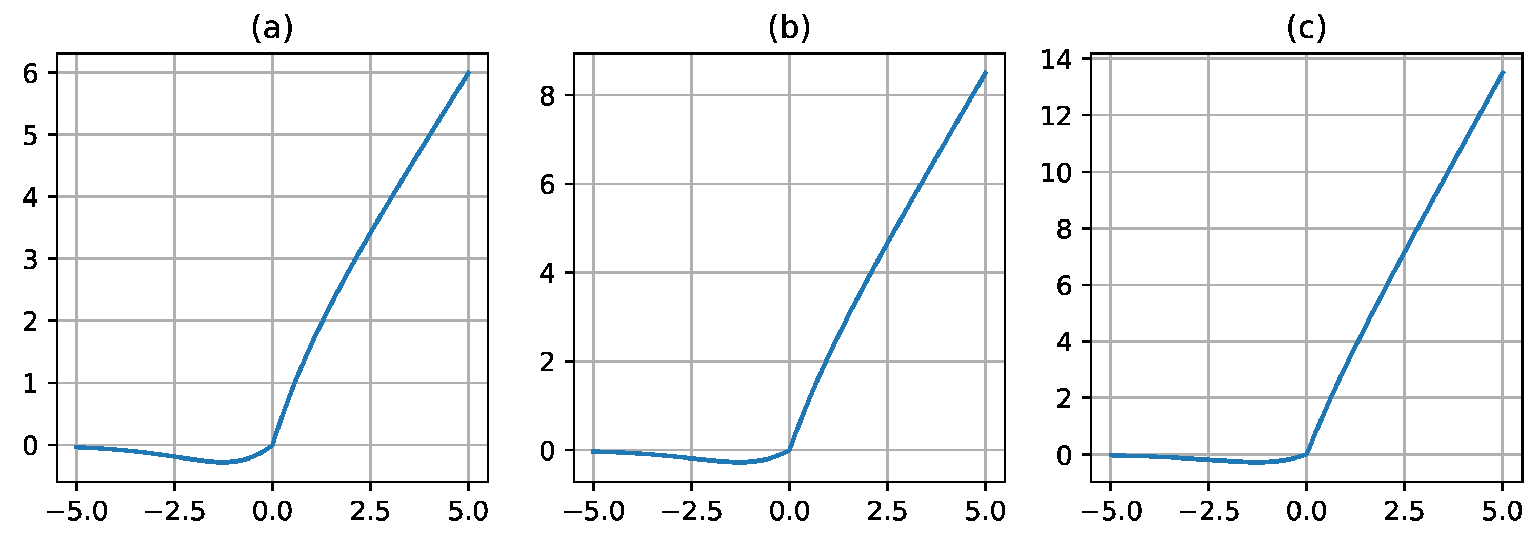
This function uses the left part of SiLU, thus getting a buffer region to the left of zero, which allows you to get a smooth output from the function near zero. The right part is similar to an ordinary ReLU, but more smoothed, because it uses

| e^{- x} - 1 |

. In addition to the exponent, we use the coefficient n to be able to change the slope of the linear part of the activation function (the coefficient at x). Figure 2 shows different variants of the DELU activation function with different values of parameter n.

3.3. LinComb and NormLinComb

In this section, we discuss the LinComb and NormLinComb activation functions, which are defined by Equation 5 and Equation 6 correspondingly.

L i n C o m b (x) = \sum_{i = 0}^{n} w_{i} F_{i} (x)

(5)

N o r m L i n C o m b (x) = \frac{\sum_{i = 0}^{n} w_{i} F_{i} (x)}{∣ ∣ W ∣ ∣}

(6)

Here

w_{i}

is a trainable parameter,

F_{i}

is an activation function, n is the number of terms in a linear combination.

NormLinComb is an analog of linear combination from the [10], but with other set of functions in the linear combination.

We chose (ReLU, Sigmoid, Tanh, SoftSign) set of functions because it does not significantly reduce the speed of the model and gives a good result.

R e L U (x) = m a x (0, x)

(7)

T a n h (x) = \frac{e^{x} - e^{- x}}{e^{x} + e^{- x}}

(8)

S o f t S i g n (x) = \frac{x}{1 + | x |}

(9)

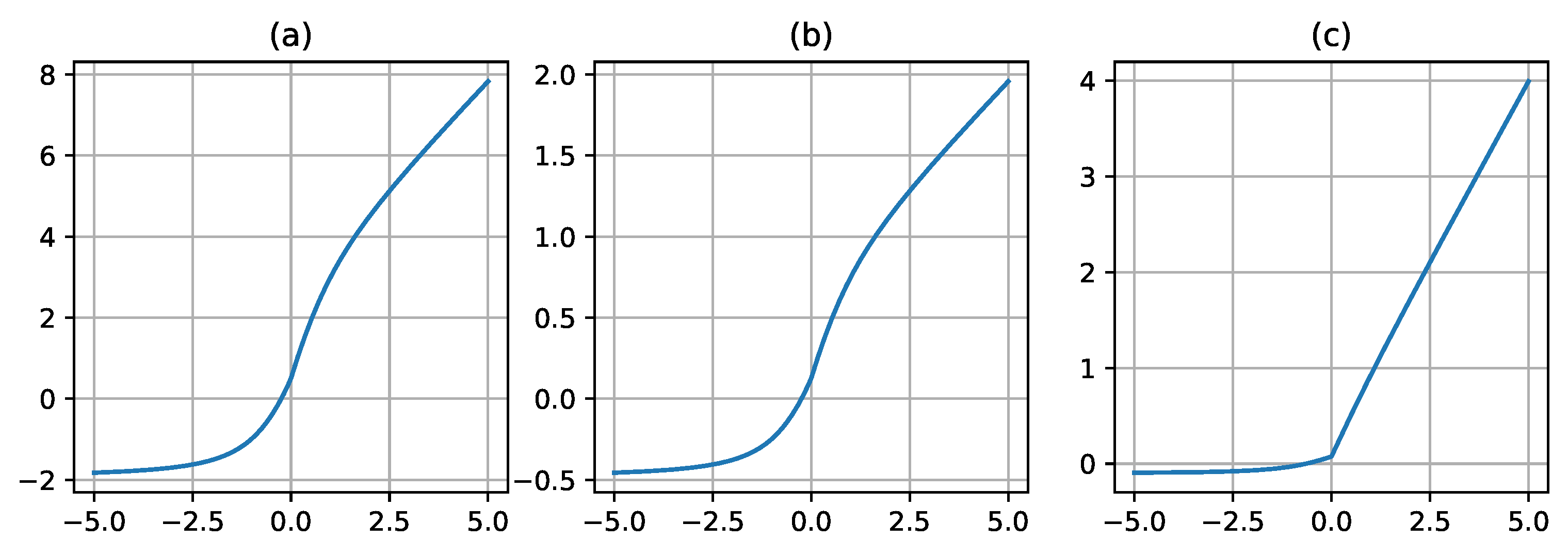
These functions implement the idea of combining various activation functions as one linear combination with all coefficients for the functions as trainable parameters, allowing the model to independently determine the contribution of each of the functions during training. Thus, this activation function is more flexible and can adapt to the data, but, unfortunately, compared to other developed functions, the speed of the model reduces significantly.

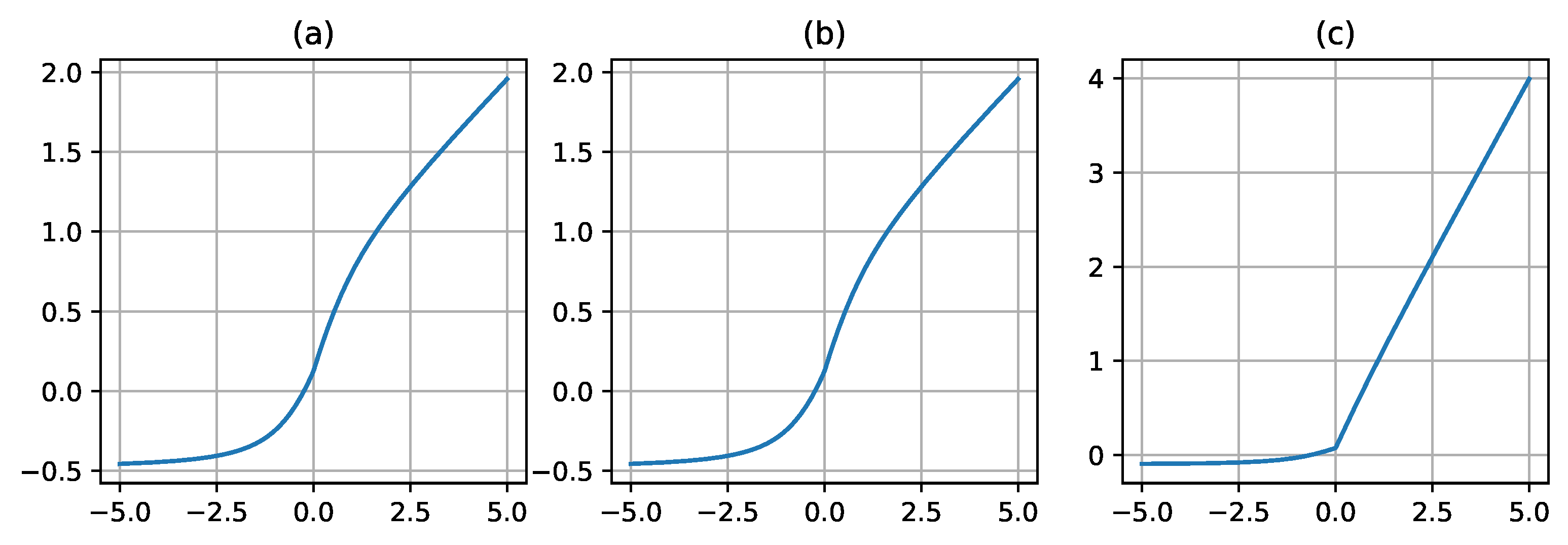
In the NormLinComb activation function the linear combination is normalized using the weight’s norm after being obtained. Figure 3 and Figure 4 show different variants of the LinComb and NormLinComb activation functions with different values of trainable parameters.

3.4. ReLUN

In this section, we discuss the ReLUN activation function, which is defined by Equation 10.

R e L U N (x) = m i n (m a x (0, x), n)

(10)

R e L U 6 (x) = m i n (m a x (0, x), 6)

(11)

Here n is a trainable parameter.

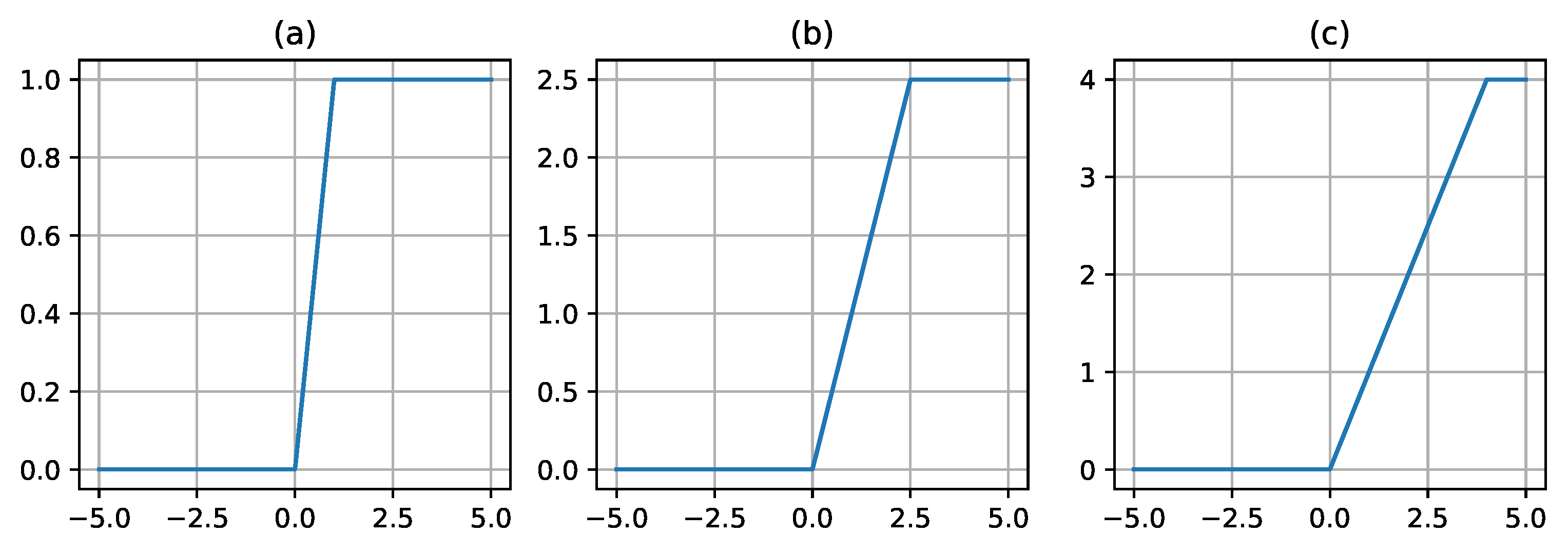
ReLUN is a trainable version for ReLU6, which is defined by Equation 11. During the use of this activation function, we allow the model to “select” the maximum possible value itself, which allows us to get rid of undesirably high values after each layer where this activation function is used. However, this type of function does not get rid of all the problems of the original ReLU. Figure 5 shows different variants of the ReLUN activation function with different values of the parameter n.

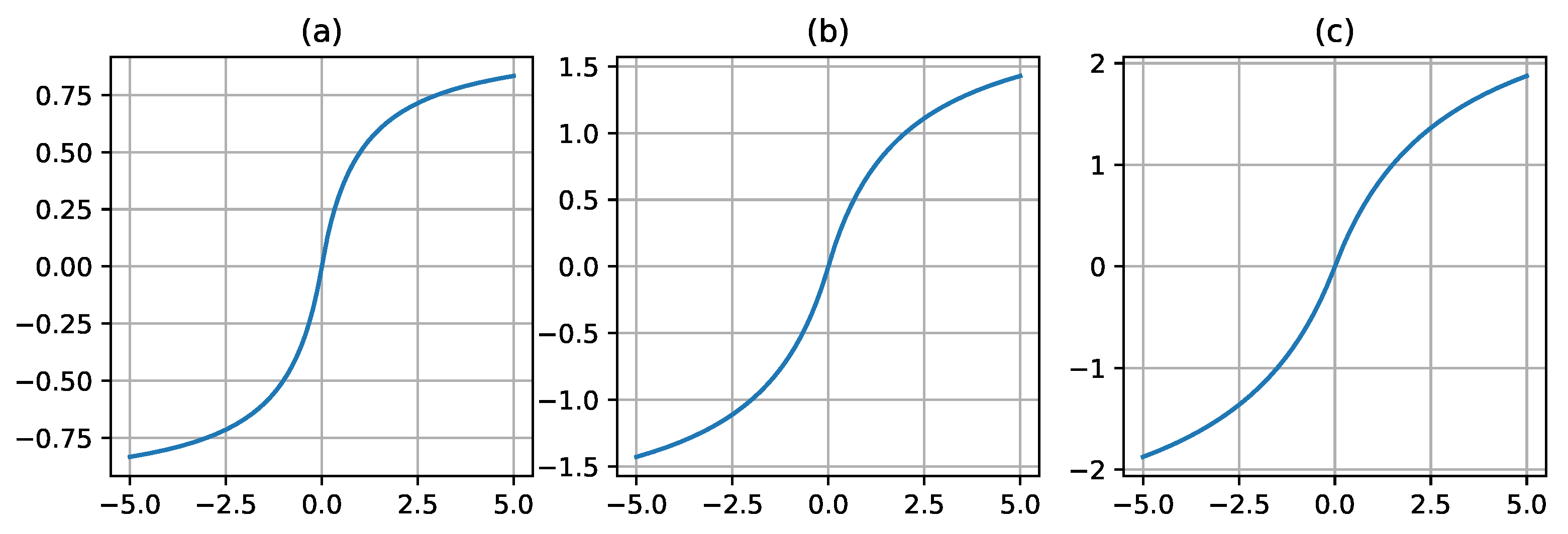
3.5. ScaledSoftSign

In this section, we discuss the ScaledSoftSign activation function, which is defined by Equation 12.

S c a l e d S o f t S i g n (x) = \frac{α x}{β + | x |}

(12)

Here

α

and

β

are trainable parameters.

The developed function is a scaled version of SoftSign, which is defined in Equation 9, the

α

parameter allows you to make a function with different ranges of values on the y axis, and

β

allows you to control the rate of transition between signs. Figure 6 shows different variants of the ScaledSoftSign function with different values of the

α

and

β

parameters.

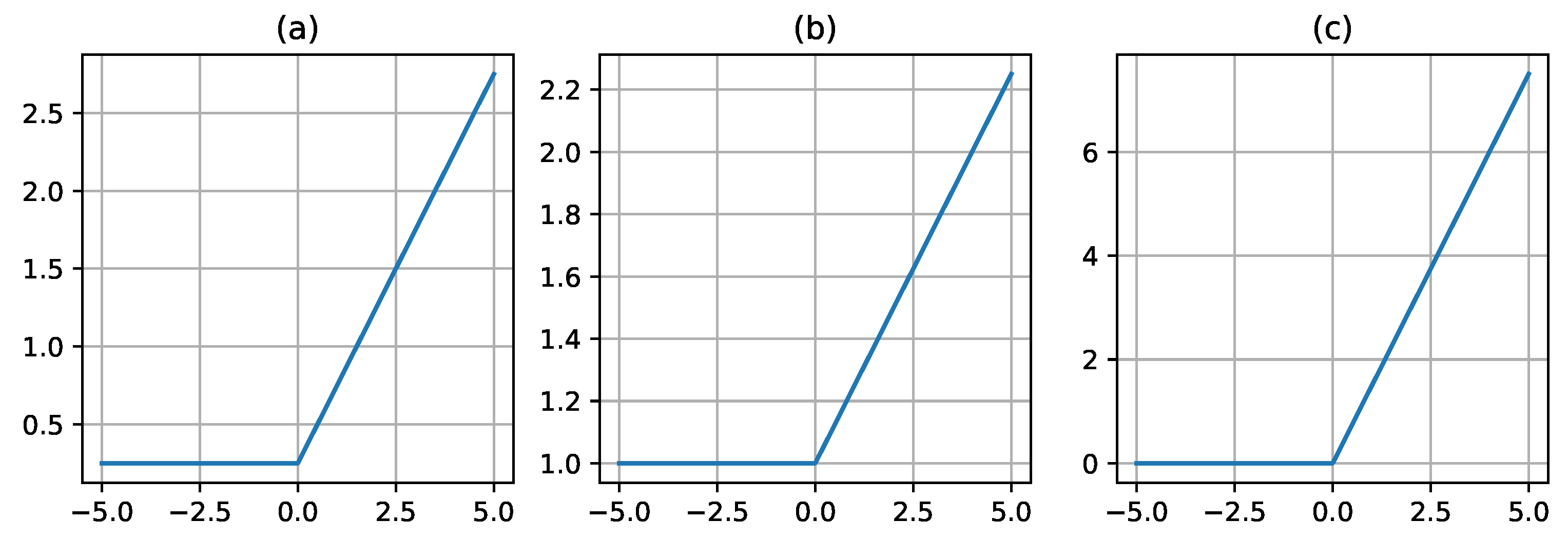
3.6. ShiLU

In this section, we discuss the ShiLU activation function, which is defined by Equation 13.

S h i L U (x) = α R e L U (x) + β

(13)

Here ReLU is the activation function, which is defined by Equation 7.

α

and

β

are trainable parameters.

This function is a trainable version of the ReLU function, in which the

α

parameter allows you to control the slope of the linear function x on the right side of the activation function. The

β

parameter allows you to shift our activation function relative to the y axis. The derivative of our function remains computationally efficient, but we allow the model to “select” the form of our function, which can improve the model performance. However, this type of function doesn’t get rid of the problems of the original ReLU. Figure 7 shows different variants of the ShiLU activation function with different values of the

α

and

β

parameters.

4. Experiments

In this section, we performed a number of experiments to test the performance of the proposed activation functions. We compare the performance of the proposed activation functions against ReLU and each other. This function was chosen because of its frequent usage in deep neural networks. The experiments were carried out on the CIFAR-10 [7] and MNIST [12] datasets. ResNet [8] and DNN (Deep Neural Network) models were used.

4.1. Dataset

CIFAR-10. The CIFAR-10 dataset consists of 60000 32x32 color images in 10 classes (airplane, automobile, bird, cat, deer, dog, frog, horse, ship, truck), with 6000 images per class. There are 50000 training images and 10000 test images. All images belong to only one unique class, for example, there are no intersections between the truck and automobile class.

MNIST. The MNIST handwritten digits dataset consists of 70000 28x28 grayscale images in 10 classes, has a training set of 60000 examples, and a test set of 10000 examples.

4.2. Model

ResNet. We used ResNet models for all tests on the CIFAR-10 dataset. Since we were using the CIFAR-10 dataset, we could not use the popular ResNet-18, ResNet-34 models, so we used the ResNet-20, ResNet-32, ResNet-44, ResNet-56 models described in the original ResNet [8] article. We modified these models and called them ResNet-8, ResNet-14 and ResNet-26 (n=1, n=2, n=4, respectively). See Table 1 for detailed architectures.

DNN. We used DNN models for all tests on the MNIST dataset. These architectures don’t have convolutional layers, only linear ones. We use DNN-2, DNN-3 and DNN-5 models (n=2, n=3, n=5, respectively). See Table 2 for detailed architectures.

4.3. Results

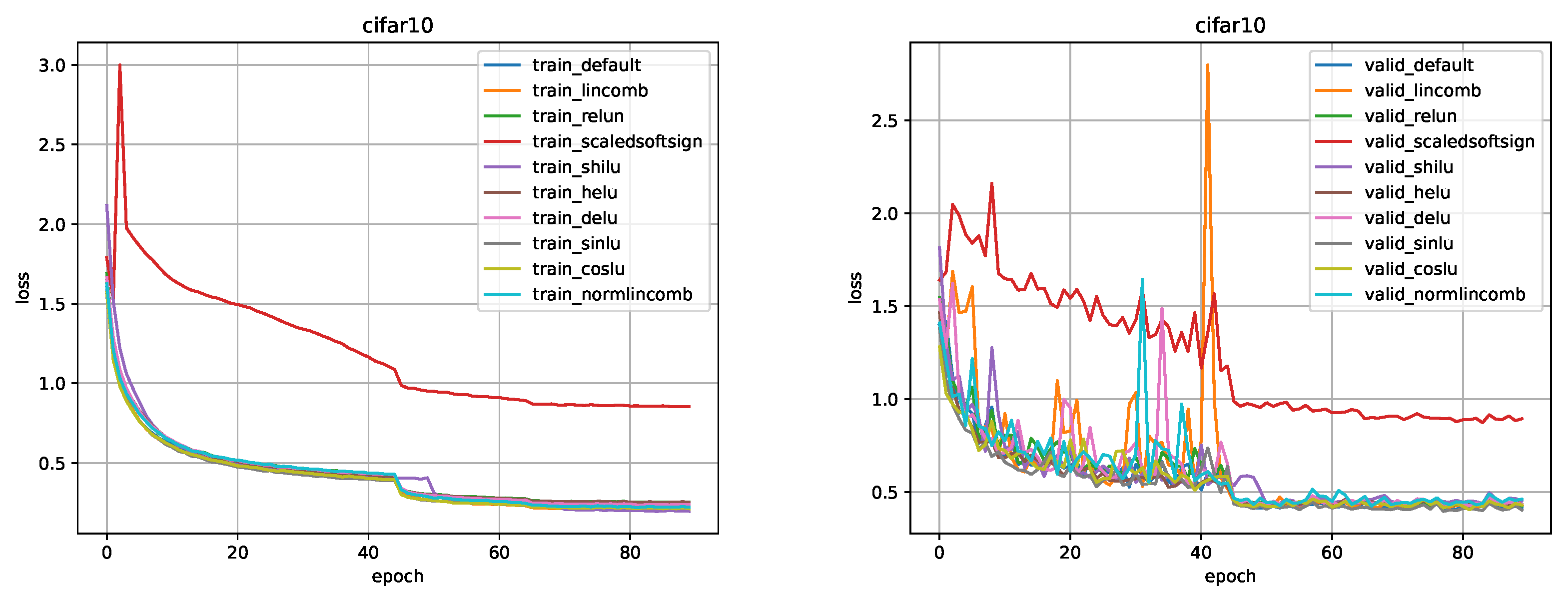
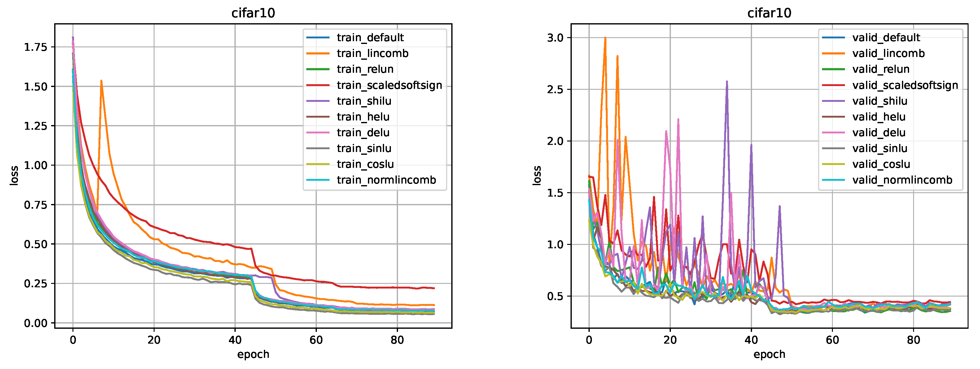
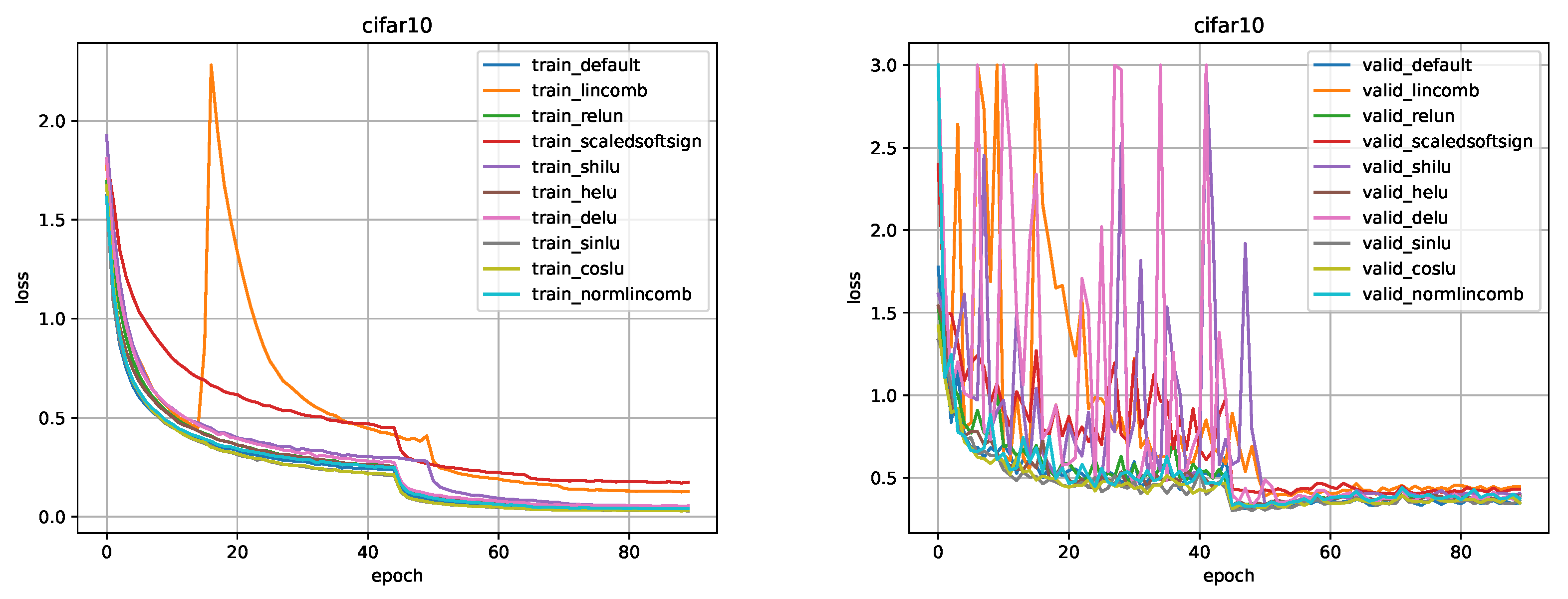
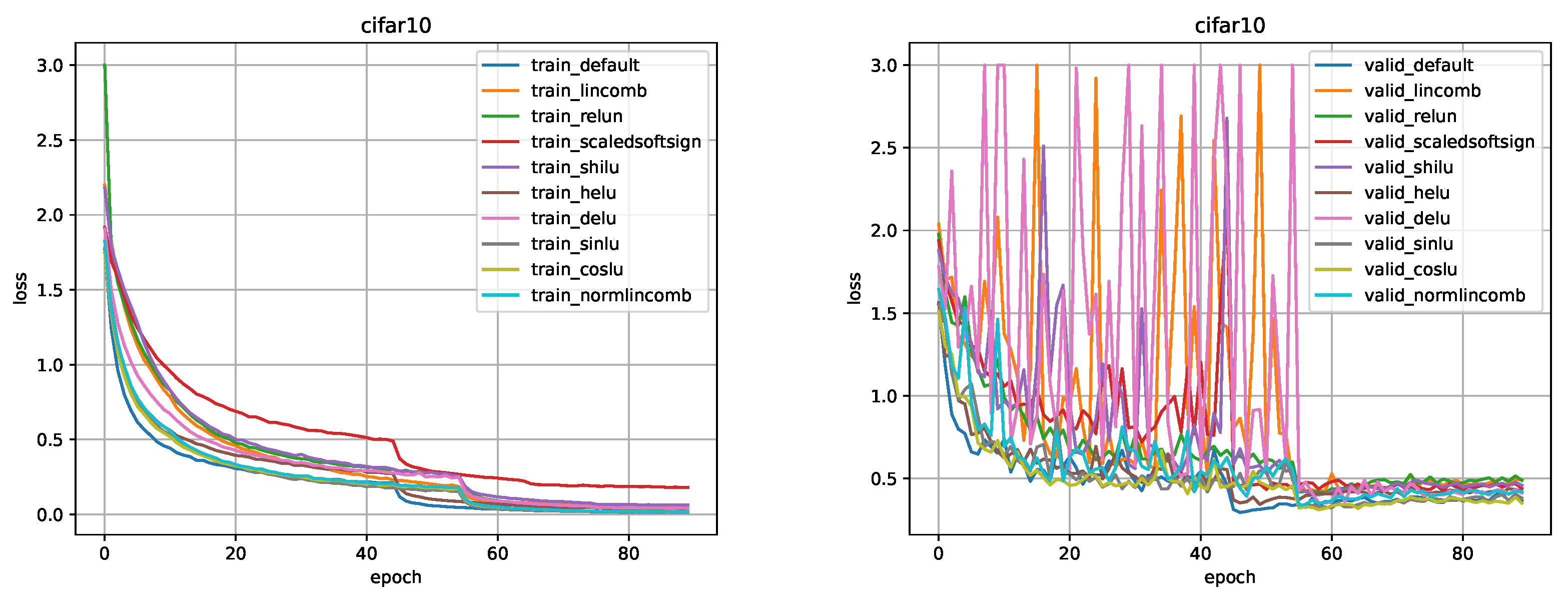
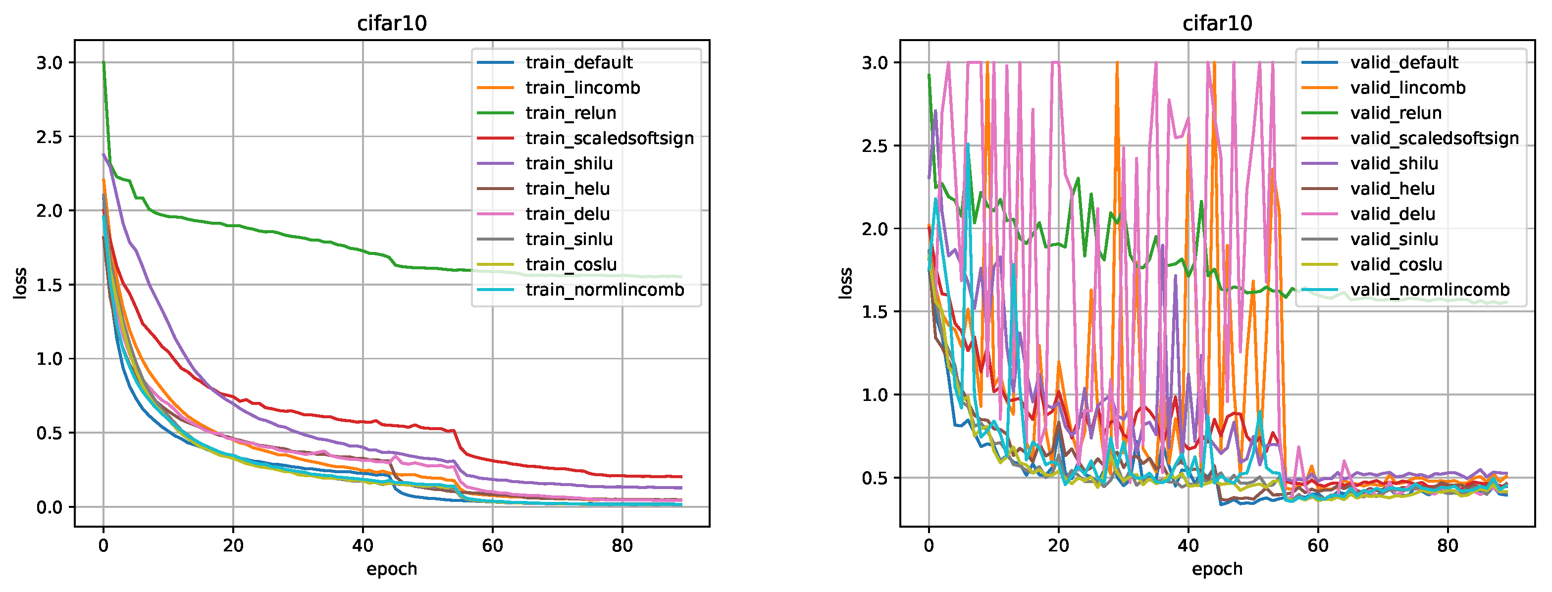
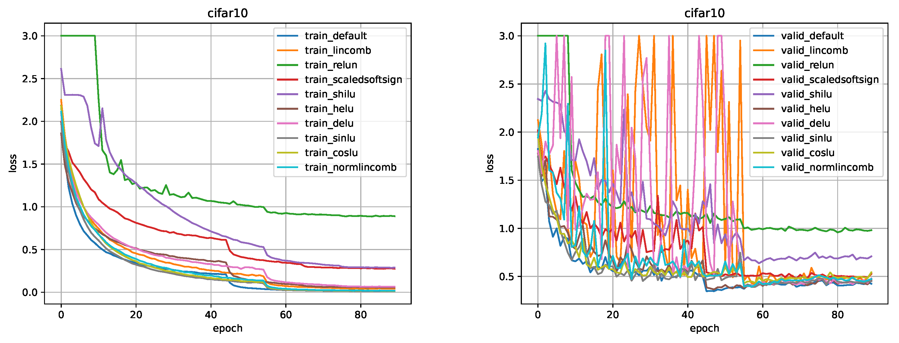
CIFAR-10. All training parameters, such as data augmentation, data splitting, learning rate, weight decay, optimizer, scheduler were taken from the original ResNet [8] article section about training on CIFAR-10 data. Figure 8, Figure 9, Figure 10, Figure 11, Figure 12, Figure 13 and Figure 14 show a comparison of the values of the loss function in training and validation stages (default is the ReLU). Comparison of metrics in training/testing is presented in Table 3.

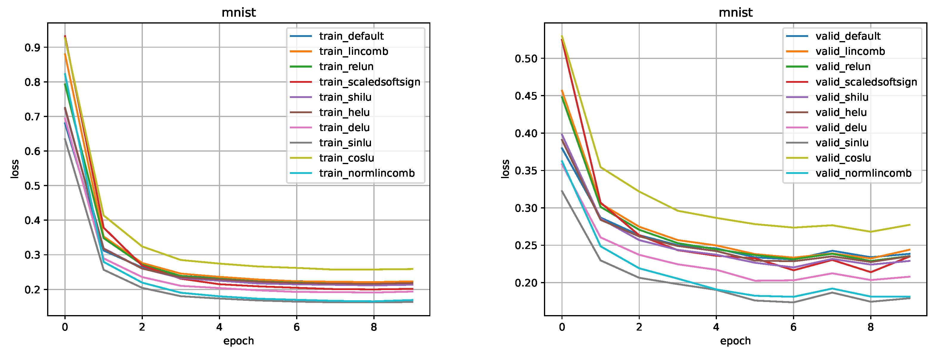
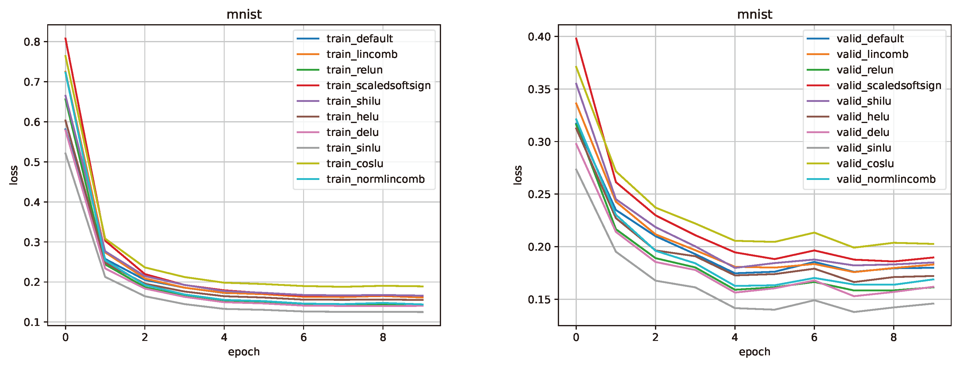
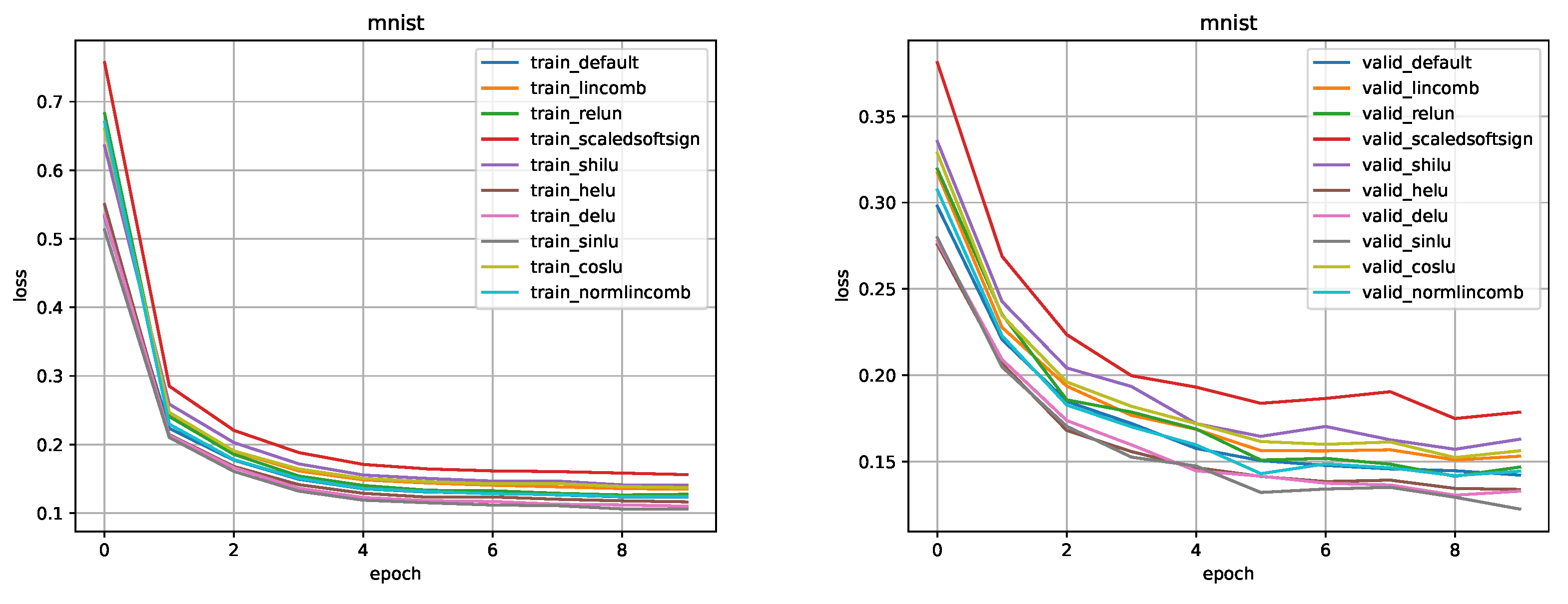
MNIST. Training parameters, such as learning rate, optimizer, scheduler were taken from the SinLU [5] article section about lightweight neural networks. Figure 15, Figure 16 and Figure 17 show a comparison of the values of the loss function in training and validation stages (default is the ReLU). Comparison of metrics in training/testing is presented in Table 4.

A c c u r a c y = \frac{T P + T N}{T P + F P + T N + F N}

(14)

Here

T P

(True Positives),

F P

(False Positives),

T N

(True Negatives),

F N

(False Negatives) are parts of the Confusion Matrix.

4.3.1. CosLU comparison

CIFAR-10. Using this activation, we obtained results comparable to ReLU. We can spot that the larger the model is, the earlier our activation function outperforms ReLU, but at the same time the moment of a significant drop in loss occurs earlier for ReLU and both activation functions allow us to obtain a comparable loss value in training and validation as a result.

MNIST. The results obtained using this activation function turned out to be slightly worse than those of the ReLU. Using CosLU for the DNN models, we failed to achieve the desirable results.

4.3.2. DELU comparison

CIFAR-10. Using this activation function, we could not get adequate results. For ResNet-8 the results were comparable to ReLU, however, the performance decreased with the expansion of the model. Also, in addition to the performance decrease, there was a strong instability on validation until the moment of a significant drop of the loss function value. We failed to achieve the desired result for DELU.

MNIST. This activation function has proven itself to be well suited for DNN models. It outperformed the ReLU in all tests, while not affecting the speed of the model. The average accuracy increase was about 0.5%.

4.3.3. LinComb and NormLinComb comparison

CIFAR-10. The LinComb activation function performed well on the ResNet-8 model, but on all other models the results turned out worse than those of the ReLU. Moreover, similarly to DELU, the problem of instability on validation was detected. The NormLinComb function managed to handle this particular problem better. The results on all ResNet models turned out to be good, some are comparable to the results of ReLU, some outperform the ReLU. It was not possible to achieve the desired result on most ResNet models using the LinComb function, with the exception of ResNet-8, however, NormLinComb function achieved the desirable results.

MNIST. The results obtained using the LinComb activation function are comparable to the results of the ReLU. On average, the accuracy decrease was 0.1%. However, all the results obtained with NormLinComb surpassed the results of the ReLU. The accuracy increase averaged 0.5%.

4.3.4. ReLUN comparison

CIFAR-10. This activation function showed results comparable to ReLU on all models except ResNet-44 and ResNet-56. We were not able to achieve significant improvement over ReLU, but there was no degradation of the results on small models.

MNIST. This activation function, as well as the DELU and NormLinComb functions, has proven itself to be well suited for DNN models. It outperformed the ReLU in all tests, the average accuracy increase was about 0.4%.

4.3.5. ScaledSoftSign comparison

CIFAR-10. This activation function showed results worse than that of the ReLU for all ResNet models.

MNIST. This activation function outperformed the ReLU on the DNN-2 model, however, with the increase in the model size the results of this function became worse in comparison with ReLU.

4.3.6. ShiLU comparison

CIFAR-10. This activation function performed well on the ResNet-8 model, outperforming ReLU. However, with the model expansion, the results deteriorated.

MNIST. The results obtained using this activation function are comparable to the results of the ReLU. On average, the accuracy decrease was 0.1%.

5. Conclusions

In this article, we have developed several activation functions with trainable parameters. We tested each function and compared them with ReLU. Results varied from one function to another. Some of them were good, some were comparable, and some were poor. We have identified one property of the majority of presented activation functions with trainable parameters, which is the larger the model becomes, the more their performance decreases in comparison to other popular functions such as ReLU. We assume that this is due to an increase in the number of layers, thereby the number of activation functions. Each function is trained independently from the others, and as a result, the performance of the model decreases. We assume that in the future these functions will find their application in some specific domains, small architectures of deep neural networks, etc. This topic remains open for further research, which will allow for a significant increase in the performance relative to the current state.

References

Nair, V., Hinton, G; Rectified Linear Units Improve Restricted Boltzmann Machines; ICML: Haifa, Israel, 2010; pp. 807–814.
Bishop, C.M. Pattern Recognition and Machine Learning; Springer: Berlin, Germany, 2006. [Google Scholar]
Maas, Andrew L, Hannun, Awni Y, and Ng, Andrew Y. Rectifier nonlinearities improve neural network acoustic models. In ICML, volume 30, 2013.
Djork-Arné Clevert, Thomas Unterthiner, Sepp Hochreiter. Fast and Accurate Deep Network Learning by Exponential Linear Units (ELUs). 2015; arXiv:1511.07289.
Paul Ashis, Bandyopadhyay Rajarshi, Yoon Jin, Geem Zong Woo, Sarkar Ram. SinLU: Sinu-Sigmoidal Linear Unit. Mathematics. 2022; 10, 337. [CrossRef]
Elfwing, S.; Uchibe, E.; Doya, K. Sigmoid-weighted linear units for neural network function approximation in reinforcement learning. Neural Netw. 2018, 107, 3–11. [Google Scholar] [CrossRef] [PubMed]
Alex Krizhevsky. Learning Multiple Layers of Features from Tiny Images. 2009.
Kaiming He, Xiangyu Zhang, Shaoqing Ren, Jian Sun. Deep Residual Learning for Image Recognition. 2015; arXiv:1512.03385.
Koushik Biswas, Sandeep Kumar, Shilpak Banerjee, Ashish Kumar Pandey. ErfAct and Pserf: Non-monotonic Smooth Trainable Activation Functions. 2009; arXiv:2109.04386.
Zhaohe Liao. Trainable Activation Function in Image Classification. 2004; arXiv:2004.13271.
Andrea Apicella, Francesco Donnarumma, Francesco Isgrò, Roberto Prevete. A survey on modern trainable activation functions. 2005; arXiv:2005.00817.
Y. LeCun, L. Y. LeCun, L. Bottou, Y. Bengio, and P. Haffner. Gradient-based learning applied to document recognition. Proc. IEEE 1998, 86, 2278–2324. [Google Scholar] [CrossRef]

Figure 1. The plot of the CosLU activation function for different values of its parameters. The subplot (a) refers to a CosLU curve with

α

=1.0,

β

=1.0; (b) refers to a CosLU curve with

α

=1.0,

β

=3.0; (c) refers to a CosLU curve with

α

=3.0,

β

=1.0.

Figure 1. The plot of the CosLU activation function for different values of its parameters. The subplot (a) refers to a CosLU curve with

α

=1.0,

β

=1.0; (b) refers to a CosLU curve with

α

=1.0,

β

=3.0; (c) refers to a CosLU curve with

α

=3.0,

β

=1.0.

Figure 2. The plot of the DELU activation function for different values of its parameter. The subplot (a) refers to a DELU curve with n=0.5; (b) refers to a DELU curve with n=1.0; (c) refers to a DELU curve with n=2.0.

Figure 3. The plot of the LinComb activation function for different values of its parameters. The subplot (a) refers to a LinComb curve with

w_{0}

=1.0 (ReLU),

w_{1}

=1.0 (Sigmoid),

w_{2}

=1.0 (Tanh),

w_{3}

=1.0 (SoftSign); (b) refers to a LinComb curve with

w_{0}

=0.25 (ReLU),

w_{1}

=0.25 (Sigmoid),

w_{2}

=0.25 (Tanh),

w_{3}

=0.25 (SoftSign); (c) refers to a LinComb curve with

w_{0}

=0.75 (ReLU),

w_{1}

=0.15 (Sigmoid),

w_{2}

=0.07 (Tanh),

w_{3}

=0.03 (SoftSign).

Figure 3. The plot of the LinComb activation function for different values of its parameters. The subplot (a) refers to a LinComb curve with

w_{0}

=1.0 (ReLU),

w_{1}

=1.0 (Sigmoid),

w_{2}

=1.0 (Tanh),

w_{3}

=1.0 (SoftSign); (b) refers to a LinComb curve with

w_{0}

=0.25 (ReLU),

w_{1}

=0.25 (Sigmoid),

w_{2}

=0.25 (Tanh),

w_{3}

=0.25 (SoftSign); (c) refers to a LinComb curve with

w_{0}

=0.75 (ReLU),

w_{1}

=0.15 (Sigmoid),

w_{2}

=0.07 (Tanh),

w_{3}

=0.03 (SoftSign).

Figure 4. The plot of the NormLinComb activation function for different values of its parameters. The subplot (a) refers to a NormLinComb curve with

w_{0}

=1.0 (ReLU),

w_{1}

=1.0 (Sigmoid),

w_{2}

=1.0 (Tanh),

w_{3}

=1.0 (SoftSign); (b) refers to a NormLinComb curve with

w_{0}

=0.25 (ReLU),

w_{1}

=0.25 (Sigmoid),

w_{2}

=0.25 (Tanh),

w_{3}

=0.25 (SoftSign); (c) refers to a NormLinComb curve with

w_{0}

=0.75 (ReLU),

w_{1}

=0.15 (Sigmoid),

w_{2}

=0.07 (Tanh),

w_{3}

=0.03 (SoftSign).

Figure 4. The plot of the NormLinComb activation function for different values of its parameters. The subplot (a) refers to a NormLinComb curve with

w_{0}

=1.0 (ReLU),

w_{1}

=1.0 (Sigmoid),

w_{2}

=1.0 (Tanh),

w_{3}

=1.0 (SoftSign); (b) refers to a NormLinComb curve with

w_{0}

=0.25 (ReLU),

w_{1}

=0.25 (Sigmoid),

w_{2}

=0.25 (Tanh),

w_{3}

=0.25 (SoftSign); (c) refers to a NormLinComb curve with

w_{0}

=0.75 (ReLU),

w_{1}

=0.15 (Sigmoid),

w_{2}

=0.07 (Tanh),

w_{3}

=0.03 (SoftSign).

Figure 5. The plot of the ReLUN activation function for different values of its parameter. The subplot (a) refers to a ReLUN curve with n=1.0; (b) refers to a ReLUN curve with n=2.5; (c) refers to a ReLUN curve with n=4.0.

Figure 6. The plot of the ScaledSoftSign activation function for different values of its parameter. The subplot (a) refers to a ScaledSoftSign curve with

α

=1.0,

β

=1.0; (b) refers to a ScaledSoftSign curve with

α

=2.0,

β

=2.0; (c) refers to a ScaledSoftSign curve with

α

=3.0,

β

=3.0.

Figure 6. The plot of the ScaledSoftSign activation function for different values of its parameter. The subplot (a) refers to a ScaledSoftSign curve with

α

=1.0,

β

=1.0; (b) refers to a ScaledSoftSign curve with

α

=2.0,

β

=2.0; (c) refers to a ScaledSoftSign curve with

α

=3.0,

β

=3.0.

Figure 7. The plot of the ShiLU activation function for different values of its parameter. The subplot (a) refers to a ShiLU curve with

α

=0.5,

β

=0.25; (b) refers to a ShiLU curve with

α

=0.25,

β

=1.0; (c) refers to a ShiLU curve with

α

=1.5,

β

=0.0.

Figure 7. The plot of the ShiLU activation function for different values of its parameter. The subplot (a) refers to a ShiLU curve with

α

=0.5,

β

=0.25; (b) refers to a ShiLU curve with

α

=0.25,

β

=1.0; (c) refers to a ShiLU curve with

α

=1.5,

β

=0.0.

Figure 8. Comparison for ResNet-8 model on the CIFAR-10 dataset.

Figure 9. Comparison for ResNet-14 model on the CIFAR-10 dataset.

Figure 10. Comparison for ResNet-20 model on the CIFAR-10 dataset.

Figure 11. Comparison for ResNet-26 model on the CIFAR-10 dataset.

Figure 12. Comparison for ResNet-32 model on the CIFAR-10 dataset.

Figure 13. Comparison for ResNet-44 model on the CIFAR-10 dataset.

Figure 14. Comparison for ResNet-56 model on the CIFAR-10 dataset.

Figure 15. Comparison for DNN-2 model on the MNIST dataset.

Figure 16. Comparison for DNN-3 model on the MNIST dataset.

Figure 17. Comparison for DNN-5 model on the MNIST dataset.

Table 1. ResNet architectures for CIFAR-10. Building blocks are shown in brackets, with the numbers of blocks stacked.

layer name	output size	8-layer	14-layer	20-layer	26-layer	32-layer	44-layer	56-layer
conv1	32×32	3×3, 16, stride 1, padding 1
conv2_x	32×32	$[\begin{matrix} 3 \times 3, 16 \\ 3 \times 3, 16 \end{matrix}]$ ×1	$[\begin{matrix} 3 \times 3, 16 \\ 3 \times 3, 16 \end{matrix}]$ ×2	$[\begin{matrix} 3 \times 3, 16 \\ 3 \times 3, 16 \end{matrix}]$ ×3	$[\begin{matrix} 3 \times 3, 16 \\ 3 \times 3, 16 \end{matrix}]$ ×4	$[\begin{matrix} 3 \times 3, 16 \\ 3 \times 3, 16 \end{matrix}]$ ×5	$[\begin{matrix} 3 \times 3, 16 \\ 3 \times 3, 16 \end{matrix}]$ ×7	$[\begin{matrix} 3 \times 3, 16 \\ 3 \times 3, 16 \end{matrix}]$ ×9
conv3_x	16×16	$[\begin{matrix} 3 \times 3, 32 \\ 3 \times 3, 32 \end{matrix}]$ ×1	$[\begin{matrix} 3 \times 3, 32 \\ 3 \times 3, 32 \end{matrix}]$ ×2	$[\begin{matrix} 3 \times 3, 32 \\ 3 \times 3, 32 \end{matrix}]$ ×3	$[\begin{matrix} 3 \times 3, 32 \\ 3 \times 3, 32 \end{matrix}]$ ×4	$[\begin{matrix} 3 \times 3, 32 \\ 3 \times 3, 32 \end{matrix}]$ ×5	$[\begin{matrix} 3 \times 3, 32 \\ 3 \times 3, 32 \end{matrix}]$ ×7	$[\begin{matrix} 3 \times 3, 32 \\ 3 \times 3, 32 \end{matrix}]$ ×9
conv4_x	8×8	$[\begin{matrix} 3 \times 3, 64 \\ 3 \times 3, 64 \end{matrix}]$ ×1	$[\begin{matrix} 3 \times 3, 64 \\ 3 \times 3, 64 \end{matrix}]$ ×2	$[\begin{matrix} 3 \times 3, 64 \\ 3 \times 3, 64 \end{matrix}]$ ×3	$[\begin{matrix} 3 \times 3, 64 \\ 3 \times 3, 64 \end{matrix}]$ ×4	$[\begin{matrix} 3 \times 3, 64 \\ 3 \times 3, 64 \end{matrix}]$ ×5	$[\begin{matrix} 3 \times 3, 64 \\ 3 \times 3, 64 \end{matrix}]$ ×7	$[\begin{matrix} 3 \times 3, 64 \\ 3 \times 3, 64 \end{matrix}]$ ×9
	8×8	flatten, 10-d fc

Table 2. DNN architectures for MNIST.

DNN-2	DNN-3	DNN-5
flatten
fc 392-d		fc 512-d
	fc 392-d	fc 256-d
	fc 196-d	fc 128-d
		fc 64-d
fc 10-d

Table 3. Accuracy (in %, Equation 14) comparison (train/test) for the CIFAR-10 dataset.

model name	ReLU	CosLU	DELU	LinComb	NormLinComb	ReLUN	ScaledSoftSign	ShiLU
ResNet-8	92.4 / 86.7	93.3 / 86.5	92.5 / 85.6	93.5 / 86.3	92.8 / 86.3	92.1 / 86.3	70.0 / 69.9	93.7 / 86.1
ResNet-14	98.1 / 89.2	98.4 / 89.0	97.7 / 88.6	97.0 / 87.5	98.0 / 88.3	97.9 / 88.6	93.2 / 86.0	98.0 / 88.6
ResNet-20	99.2 / 90.1	99.4 / 90.4	98.8 / 88.7	96.3 / 87.3	99.2 / 89.8	99.0 / 89.4	94.9 / 86.6	98.7 / 89.2
ResNet-26	99.6 / 90.7	99.6 / 91.1	99.0 / 89.5	93.4 / 84.6	99.7 / 90.7	99.0 / 88.8	94.9 / 86.3	98.3 / 88.2
ResNet-32	99.7 / 90.9	99.7 / 90.9	99.1 / 88.8	98.8 / 87.7	99.7 / 90.0	99.2 / 87.1	94.4 / 85.6	98.4 / 87.5
ResNet-44	99.7 / 89.8	99.8 / 90.5	99.0 / 89.6	99.1 / 87.6	99.8 / 90.0	43.7 / 44.7	93.8 / 86.1	96.3 / 85.4
ResNet-56	99.8 / 89.4	99.8 / 88.8	98.4 / 88.8	99.2 / 87.9	99.7 / 89.1	69.7 / 67.1	91.1 / 84.4	91.1 / 78.7

Table 4. Accuracy (in %, Equation 14) comparison (train/test) for the MNIST dataset.

model name	ReLU	CosLU	DELU	LinComb	NormLinComb	ReLUN	ScaledSoftSign	ShiLU
DNN-2	93.6 / 96.0	92.9 / 95.7	94.4 / 96.4	93.4 / 96.0	95.1 / 96.5	94.0 / 96.3	94.0 / 96.2	93.8 / 96.0
DNN-3	95.1 / 96.7	94.3 / 96.4	95.7 / 97.0	95.0 / 96.7	95.5 / 96.8	95.7 / 97.0	95.0 / 96.4	94.9 / 96.6
DNN-5	96.1 / 97.1	95.7 / 96.9	96.6 / 97.2	95.7 / 97.0	96.2 / 97.1	96.2 / 97.1	95.3 / 96.3	95.6 / 96.9

Disclaimer/Publisher’s Note: The statements, opinions and data contained in all publications are solely those of the individual author(s) and contributor(s) and not of MDPI and/or the editor(s). MDPI and/or the editor(s) disclaim responsibility for any injury to people or property resulting from any ideas, methods, instructions or products referred to in the content.

© 2023 by the authors. Licensee MDPI, Basel, Switzerland. This article is an open access article distributed under the terms and conditions of the Creative Commons Attribution (CC BY) license (http://creativecommons.org/licenses/by/4.0/).

Copyright: This open access article is published under a Creative Commons CC BY 4.0 license, which permit the free download, distribution, and reuse, provided that the author and preprint are cited in any reuse.

MDPI Initiatives

Important Links

Choose an area of interest and we will send you notifications of new preprints at your preferred frequency.

Disclaimer

Trainable Activations for Image Classification

Abstract

1. Introduction

2. Related Work

3. Proposed Approach

3.1. CosLU

3.2. DELU

3.3. LinComb and NormLinComb

3.4. ReLUN

3.5. ScaledSoftSign

3.6. ShiLU

4. Experiments

4.1. Dataset

4.2. Model

4.3. Results

4.3.1. CosLU comparison

4.3.2. DELU comparison

4.3.3. LinComb and NormLinComb comparison

4.3.4. ReLUN comparison

4.3.5. ScaledSoftSign comparison

4.3.6. ShiLU comparison

5. Conclusions

References

MDPI Initiatives

Important Links

Subscribe