Novel Learning for Control of Nonlinear Spacecraft Dynamics

Preprint

Article

Novel Learning for Control of Nonlinear Spacecraft Dynamics

Altmetrics

Downloads

180

Views

104

Comments

A peer-reviewed article of this preprint also exists.

This version is not peer-reviewed

Submitted:

24 January 2023

Posted:

26 January 2023

You are already at the latest version

Alerts

Abstract

With correct dynamic system parameters (embodied in self-awareness statements), a controller can provide precise signals for tracking desired state trajectories. If dynamic system parameters are initially guessed incorrectly, a learning method may be used to find the correct parameters. In the deterministic artificial intelligence method, self-awareness statements are formed as mathematical expressions of the governing physics. When the nonlinear, coupled expressions are precisely parameterized as the product of known matrix components and unknown victrix (i.e., a regression form) tracking errors may be projected onto the known matrix to update the unknown victrix in an optimal form (in a two-norm sense). In this work, a modified learning method is proposed and proved to have global convergence of both state error and parameter estimation error. The modified learning method is compared with those in the prequels using simulation experiments of three-dimensional rigid body dynamic rotation motion. The modified approach is two magnitudes better than the methods in the prequels in terms of state error convergence.

Keywords:

Subject: Engineering - Mechanical Engineering

1. Introduction

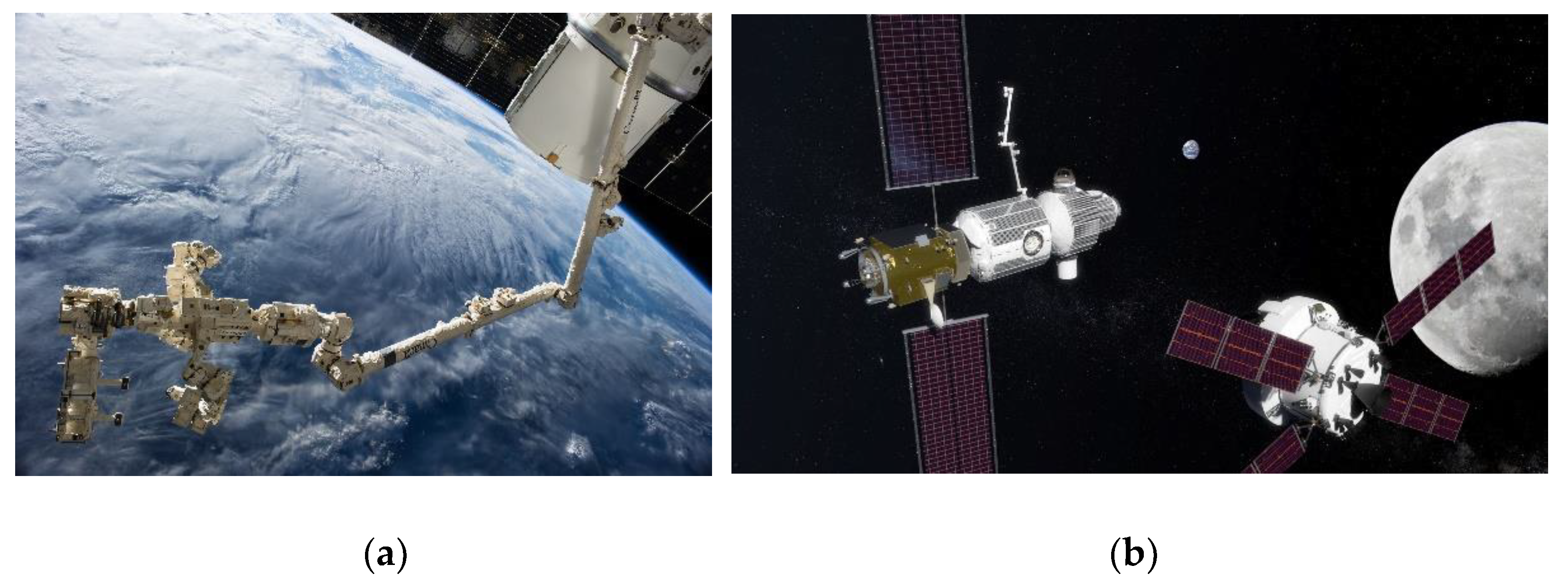
Consider intricate robotic operations in low-earth orbit near the space station as displayed in Figure 1, where considerable human intervention is available. Next contemplate the requirements to autonomously do such operations in far distant cis-lunar orbits. The latter systems must be able to learn in real-time dynamic changes that occur when the space robot grasps and grapples targeted spacecraft. Dynamics and control issues associated with rendezvous in Cis-lunar space near rectilinear halo orbits were investigated in [1] where a fully-safe, automatic rendezvous strategy was developed between a passive vehicle and an active one orbiting around the Earth–Moon L2 Lagrangian point.

Bando, et. al, [5] proposed a chattering attenuation sliding mode control utilizing the eigen structure of the linearized flow around a libration point of the Earth-Moon circular restricted three-body problem, and this novel article serves as a reminder of the prevalence of linearization when dealing with multiple, coupled nonlinear equations. In 2021, Colombia presented a guidance, navigation and control framework for 6 degrees of freedom (6DOF) coupled Cislunar rendezvous and docking, and the article highlighted the importance of dealing with full, coupled translational-rotational dynamics of multi-body (i.e., highly flexible) dynamics seeking guaranteed coupled-state estimation [6]. Immediately that same year [7], new techniques for highly flexible multi-body space robotics were proposed as a competing narrative to the just-proposed “whiplash compensation” of flexible space robotics [8]. China now has two robotic arms attached to its space station [9], where large robotic arm can "crawl" along the outside of the spacecraft [10].

Meanwhile, Zhang et. al, proposed an adaptive control strategy based on the full, nonlinear equations accounting for modeling uncertainties using an adaptive neural network amidst external disturbances [11].

In 2020, deterministic artificial intelligence was proposed by Smeresky et. al. [12], which stated that the system dynamics constitute a feedforward control when paired with analytic trajectories; and when the dynamics are expressed in a canonical regression form, optimal feedback (in the two-norm sense) can aid control of spacecraft attitude. The method stems from incremental development of a common nonlinear adaptive scheme offered by Slotine [13] for spacecraft attitude control, where elements of classical feedback were eliminated in 2020 foremost applied to unmanned underwater robotics [14]. The burgeoning lineage of research continued in 2022, when Sandberg et. al. [15] compared several trajectory-generation schemes and a nominal learning method based on the regression model, where applied torque is estimated by an enhanced Luenberger observer. Very shortly afterwards, Raigoza [16] augmented Sandberg’s trajectory generators with autonomous collision avoidance. In November 2022, Wilt examined efficacy in the face of simulated craft damage and environmental disturbances [17].

In prequel works [12,13,14,15,16,17], the error convergence property is obtained using the proper design of the trajectory generation process. However, if the external disturbance makes the current state deviate from the trajectory, even if the system parameter is already converged to a correct value, the trajectory will need to be re-calculated to fit the current state, so that the deterministic artificial intelligence can continue to drive the system using optimal feedforward control signal.

As a result, provided the initial error between the current state and the current desired trajectory as well as incorrect initial parameter value, the goal of the modified learning approach proposed in this manuscript is to guarantee the convergence to zero of both parameter error and the state error. This work focuses on the rotation rate control problem of a spacecraft and provided 2 ways of modification to the learning phase of the deterministic artificial intelligence algorithm and compared them with the original deterministic artificial intelligence using simulation in MATLAB^®. Moreover, the modified method can be proved to make the error converge to zero using similar way as how Slotine and Li [13] proved the stability of the non-linear system controlled by some specific feed-forward/feed-back controllers. That is, the Lyapunov candidate function is provided, and the time derivative of the candidate function can be proved to be negative with the proposed modified learning method.

Main contribution of the study. A novel, stable learning approach is proposed to enhance deterministic artificial intelligence and efficacy amidst external disturbances is evaluated.

2. Materials and Methods

2.1. Spacecraft Rotation Rate Control

The spacecraft rotation rate control problem focuses on applying torque so that the rotation rate of a spacecraft converges to the desired value. The dynamic can be described by the Euler equation (displayed in Equation (1)). Euler’s moment equations can be parameterized in canonical regression form. This full form of the coupled, nonlinear equations whose importance was highlighted by the research cited in the Introduction.

τ = I \dot{ω} + ω \times I ω = \underset{Φ}{\underset{⏟}{[\begin{matrix} \begin{matrix} {\dot{ω}}_{x} & {\dot{ω}}_{y} - ω_{x} ω_{z} & {\dot{ω}}_{z} + ω_{x} ω_{y} \end{matrix} & \begin{matrix} - ω_{y} ω_{z} & ω_{y}^{2} - ω_{z}^{2} & ω_{y} ω_{z} \end{matrix} \\ \begin{matrix} \begin{matrix} ω_{x} ω_{z} & {\dot{ω}}_{x} + ω_{y} ω_{z} & ω_{z}^{2} - ω_{x}^{2} \end{matrix} \\ \begin{matrix} - ω_{x} ω_{y} & ω_{x}^{2} - ω_{y}^{2} & {\dot{ω}}_{x} - ω_{y} ω_{z} \end{matrix} \end{matrix} & \begin{matrix} \begin{matrix} {\dot{ω}}_{y} & {\dot{ω}}_{z} - ω_{x} ω_{y} & - ω_{x} ω_{z} \end{matrix} \\ \begin{matrix} ω_{x} ω_{y} & {\dot{ω}}_{y} + ω_{x} ω_{z} & {\dot{ω}}_{z} \end{matrix} \end{matrix} \end{matrix}]}} \underset{Θ}{\underset{⏟}{\{\begin{matrix} \begin{matrix} I_{x x} \\ I_{x y} \end{matrix} \\ \begin{matrix} I_{x z} \\ I_{y y} \end{matrix} \\ \begin{matrix} I_{y z} \\ I_{z z} \end{matrix} \end{matrix}\}}}

(1)

The matrix Φ is the matrix of known, which is composed of the current state and the rate of the state (ω and dω/dt). The matrix Θ is the vector of the unknown, which is composed of system parameters, in this case, the moment of inertia. The way of formulation shows that it is possible to estimate the moment of inertia with the correct measurement of the current state.

2.2. Original deterministic artificial intelligence control

The idea of deterministic artificial intelligence is that if the matrix of the unknown can be estimated and the desired trajectory of the state is given, the optimal control signal will be multiplying the desired matrix of known (Φ_d), which includes the information of the current desired state, with the best guess of the parameter (

\hat{Θ}

). This turns the system dynamic to Equation (2).

τ = Φ Θ \to u \equiv Φ_{d} \hat{Θ}

(2)

However, the

\hat{Θ}

can be incorrect or changed in the middle of operation. Therefore, a learning approach should be provided so that the vector of the unknown can converge to a correct value. The original learning approach in the space rotation rate control problem is described in Equation (3).

\dot{\hat{Θ}} = Φ^{H} (τ_{a p p l i e d} - Φ \hat{Θ})

(3)

Where

τ_{a p p l i e d}

is the controller torque output, and the capital H means the pseudo inverse of a non-square matrix. In short, this provided a way to turn the difference between the applied torque and the expected torque into the parameter error, which should be a minimal square error estimation using the information in the current time stamp. Concerning the stability of the parameter estimation, the learning of the parameter is applied incrementally.

Additionally, deterministic artificial intelligence requires a trajectory generation process to produce a trajectory that leads from the current state to the desired state. If the current state deviates undesirably from the trajectory, it is better to update the trajectory, or the error of the state may accumulate. Please be aware that the desired state of the trajectory generation is not the desired state of the controller, which follows the output of the trajectory generator by making the trajectory the desired state of the controller should follow. In this manuscript, all the “desired states” mentioned are the desired state for the controller, if not specifically noted.

2.3. Modified Learning Method, a General Version

The target of the modification is that if the learning approach can also guarantee to decrease the error in the current state when doing the parameter estimation, the chance of regenerating trajectory can be decreased because the error is kept from growing, which increases the robustness. In a general version of the modification, we consider all the systems that can be expressed in the regression form, as in Equation (2), where the information of the current state is provided in the matrix of known. To study the error of the parameters and state, the error between the desired matrix of known and the current matrix of known is noted as

ϕ

, and the error of the unknown vector is noted as

θ

. Equation (2) can therefore be turned into Equation (4). In this case, the goal becomes driving both

ϕ

and

θ

to 0 simultaneously using a modified learning method.

Φ θ + ϕ \hat{Θ} = 0 w h e r e ϕ = Φ_{d} - Φ a n d θ = Θ - \hat{Θ}

(4)

Considering the Lyapunov candidate function described in Equation (5), the function value must decrease to 0 if both

ϕ

and

θ

goes to 0. If there is a parameter update approach

\dot{θ}

that makes the candidate function globally stable, it is very likely that the error of the state

ϕ

goes to 0 together with

θ

. Equation(7) shows that if

\dot{θ}

is taken in a form of Equation(6), and considering Equation (4) and the time derivative of Equation (4), the time derivative of the Lyapunov function will be globally negative, and leads to the global stability of the system as long as the matrix G is positive definitive.

V = {\hat{Θ}}^{T} ϕ^{T} ϕ \hat{Θ} + θ^{T} θ

(5)

{\dot{θ}}^{T} = {\hat{Θ}}^{T} ϕ^{T} ((Φ {\dot{Φ}}^{H}) (Φ^{H} + Φ^{T})^{H} + (Φ^{H} + Φ^{T})^{T} G (Φ^{H} + Φ^{T}))

(6)

\frac{\dot{V}}{2} = [{\hat{Θ}}^{T} ϕ^{T} Φ {\dot{Φ}}^{H} - {\dot{θ}}^{T} Φ^{H} - {\dot{θ}}^{T} Φ^{T}] ϕ \hat{Θ} = {\hat{Θ}}^{T} ϕ^{T} (Φ^{H} + Φ^{T})^{T} G (Φ^{H} + Φ^{T}) ϕ \hat{Θ}

(7)

The modified learning method provided here guarantees that the Lyapunov function always goes to zero. However, if the rank of the matrix of known is not as much as the number of the unknown parameter, it is possible that the state won’t converge when the Lyapunov function goes to zero. In the target application in this manuscript, the rank of the matrix of known is 3 while the parameter number in the vector of unknown is 6, this makes the learning method provided unable to guarantee convergence. One example is that when the unknown parameter happens to be correct while the state error exists, the state error will not be going to be zero. This can be seen in Equation (2) that when

\hat{Θ} = Θ

, the term

{\hat{Θ}}^{T} ϕ^{T} = {\hat{Θ}}^{T} {(Φ_{d} - Φ)}^{T}

will always be 0. When Φ has smaller rank than the number of unknowns, it is possible that

{\hat{Θ}}^{T} ϕ^{T}

=0 when

ϕ

is not zero.

Another concern of using this method is that the calculation of

\dot{Φ}

is prone to noises and will cause latency in the real-time calculation because it requires the knowledge of the double derivative of the rotation rate, which generally requires special treatments like the smoothing process.

2.4. Modified Learning Method, a Specific Version

To avoid the problem mentioned in 2.3, mainly the rank issue of the known matrix, a specific version of the modified learning method is provided for the rotation rate controller. The non-regression form of the system dynamic is considered in Equation (8), and the modified learning method is provided in Equation (10) which utilizes both the state error as well as parameter error. Also, the character “i” means the error in the inertia matrix in a 3*3 form rather than in a 1*6 unknown vector. The torque input to the system is slight modified from

ω_{d} \times I ω_{d}

ω_{d} \times I ω

, which improves the global stability but won’t affect the feed forward optimality in the deterministic artificial intelligence much when the state is very close to the desired value.

I \dot{ω} + ω \times I ω = \hat{I} {\dot{ω}}_{d} + ω_{d} \times I ω w h e r e \hat{i} = \hat{I} - I a n d ω' = ω - ω_{d}

(8)

I {\dot{ω}}^{'} = - (ω^{'} \times I ω_{d} + ω^{'} \times I ω^{'}) + (i^{' {\dot{ω}}_{d}} + ω_{d} \times i ω_{d} + ω_{d} \times i ω^{'}) = C ω^{'} + K θ

(9)

\dot{θ} = - Q ω^{'} - R θ

(10)

The Equation (8) is rearranged to Equation (9), and the

θ

, again, means the inertia in a unknown vector form. To proof the global convergence of both state error

ω'

and parameter error

θ

, another Lyaponuv function (Equation (11)) is provided, which have a physical meaning close to the square error of the whole system, where the state square error is weighted by the inertia. If the Q term in Equation (10) is the transpose of K term in Equation (9), and the R term in Equation (10) is positive definite, the Lyapunov function will be stable globally, as shown in Equation (12), and can achieve zero state error and parameter error is guaranteed. Finally, the parameter vector is chosen based on Equation (13), derived from Equation (4), and the value is used for modified learning method in Equation (10).

V = {ω^{'}}^{T} I ω^{'} + θ^{T} θ

(11)

\frac{\dot{V}}{2} = {ω^{'}}^{T} I \dot{ω^{'}} + θ^{T} \dot{θ} = {ω^{'}}^{T} [- (ω^{'} \times I ω_{d} + ω^{'} \times I ω^{'})] \dot{ω^{'}} + θ^{T} (K^{T} - Q) ω^{'} - θ^{T} R θ = θ^{T} (K^{T} - Q) ω' - θ^{T} R θ = - θ^{T} R θ < 0

(12)

θ = - Φ^{H} ϕ \hat{Θ}

(13)

2.5. Simulation

The trajectory tracking of the rotation rate controller will be simulated. In the simulation, the trajectory is generated using arbitrary test torque, as shown in Equation (14). The controller does not possess the test torque value, but instead receives a stream of desired rotation rate and the time derivative of the rotation rate. The idea is that if the deterministic artificial intelligence can track the test trajectory, it should also be able to track any trajectory generated by another trajectory planner.

I {\dot{ω}}_{d} + ω_{d} \times I ω_{d} = τ_{t e s t}

(14)

Two types of performance matrices are considered: norm ratio of the state error, and the norm ratio of the parameter error, in Equation (16). The result is plotted in Section 3.

S t a t e e r r o r n o r m r a t i o = \ln (\frac{| | ω' | |_{2}^{2}}{| | ω_{d} | |_{2}^{2}}) P a r a m e t e r e r r o r n o r m r a t i o = \frac{| | θ' | |_{2}^{2}}{| | Θ | |_{2}^{2}}

(15)

3. Results

In this section, simulation results of the rotation rate problem (section 2.1) under different condition is presented, and the performance of both types of modification (general version in section 2.3 and specific version in 2.4) is compared with the original deterministic artificial intelligence (section 2.2) learning approach.

3.1. Performance Comparison without the Product of Inertia

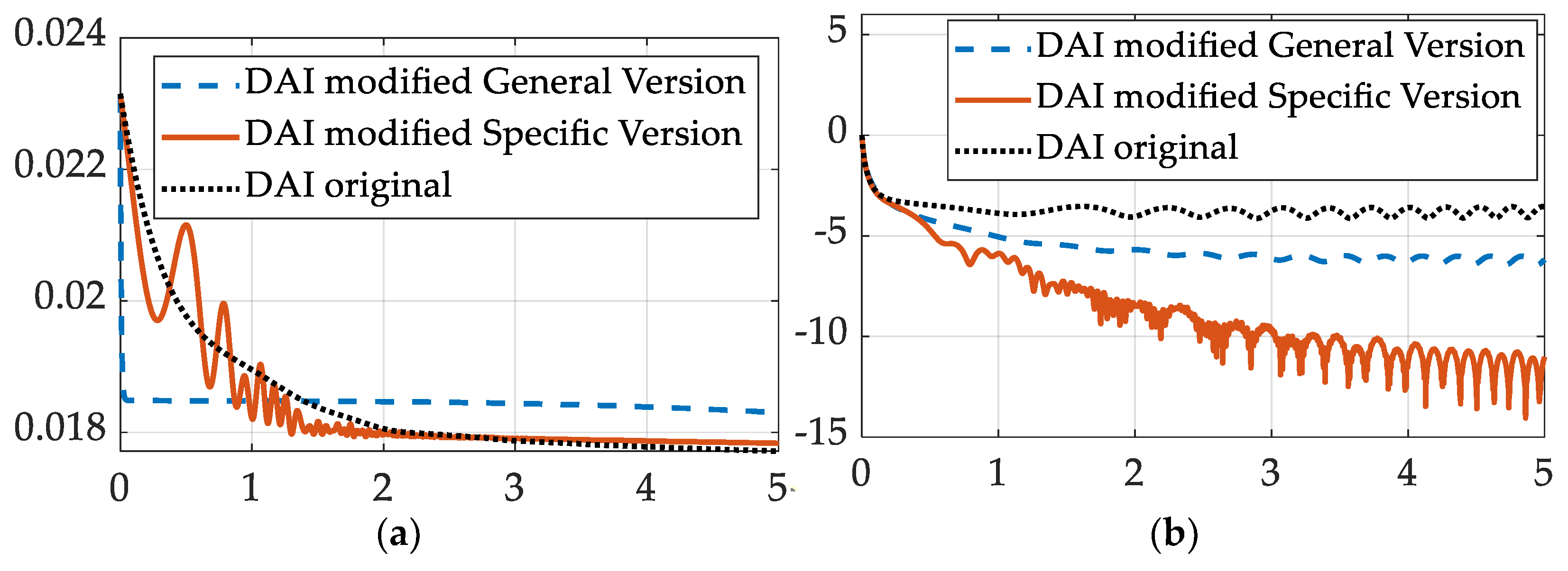
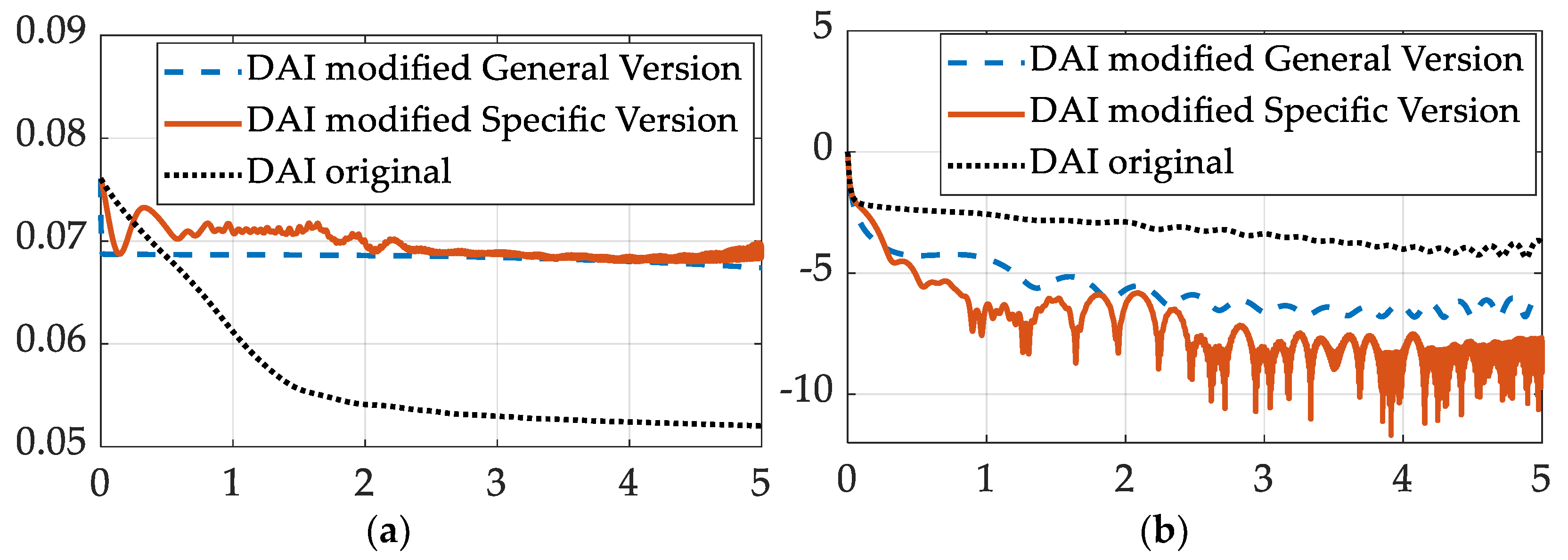
This case aims at testing the learning method when there is no product of inertia value in both the system's true parameter and the initial estimation of the unknown vector. The initial condition and the system parameters are listed in Table 1. The norm ratio of the state error and parameter error is shown in Fig. 1. Also, the G in Equation (7) and the R in Equation (10) will be a scaler “r” multiplied by a 6*6 identity matrix, and this form of G and R will be used in all the cases presented in this manuscript.

Figure 1. The convergence of the parameter error and state error. (a) Parameter error norm ratio on the ordinant versus time in seconds on the abscissa. (b) State error norm ratio on the ordinant versus time in seconds on the abscissa.

3.2. Performance Comparison with the Product of Inertia

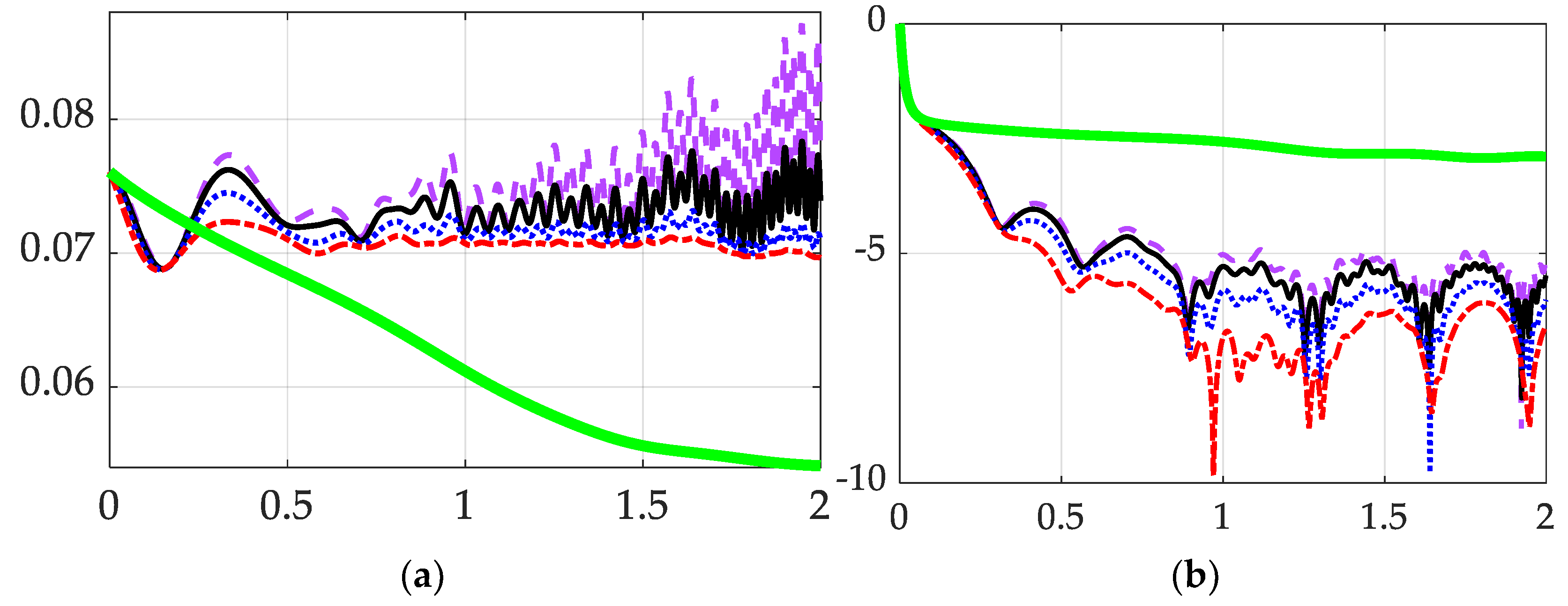
This case is similar to section 3.1, but the product of inertia values in both the system's true parameter and the initial estimation of the unknown vector is not zero. The initial condition and the system parameters are listed in Table 3. The norm ratio of the state error and parameter error is shown in Figure 2.

3.3. Performance Comparison with Different r value

This case shows for the modified learning method (Specific Version) how the r value, which can be seen as the “magnitude” of the G in Equation (7) and the R in Equation (10), affects the final result. The initial condition and parameters used in this case are identical to case 3.2 and can be checked in Table 3, except for the r value.

4. Discussion

In sections 3.1 and 3.2, the modified learning method yields better state error convergence than the original method. For the specific version of the modified method, the final state error norm ratio is about 2 magnitudes smaller (rough order

\times 10^{- 8}

compared with

\times 10^{- 3}

) than the original learning method, due to the data are shown in both Figure 1 and Figure 2.

In section 3.1, all the learning methods yield similar convergence rate of the parameter error when the moment of inertia matrix doesn’t contain the product of inertia terms, as shown in the left part of Figure 1. However, when the moment of inertia matric contains nonzero product of inertia, as has been done in section 3.2, the left part of Figure 2 shows that the modified methods are not better than the original method.

Table 5. Percent performance enhancement: Convergence of inertia estimation and tracking errors.

Figure of merit	Original method (prequels)	Proposed version general	Proposed versionspecific
Parameter error mean	0%	42%	53%
Parameter error deviation	0%	16%	100%
Mean tracking error	0%	–77%	–99%
Tracking error deviation	0%	–91%	–96%

In section 3.3, Figure 3 shows that when the magnitude of R in Equation (10) goes bigger, the convergence rate also increases. Because Equation (12) states that the convergence rate of the Lyapunov function (Equation (11)) is only determined by the size of R and

θ

, the result in section 3.3 is reasonable.

Table 6. Percent performance enhancement: Convergence of inertia estimation and tracking errors.

Figure of merit	Original method (prequels)	Modified with r = 0.5	Modified with r = 1	Modified with r = 2	Modified with r = 4
Parameter error mean	0.00%	-42.11%	-40.89%	-39.68%	-38.06%
Parameter error deviation	0.00%	-146.77%	-119.35%	-92.74%	-75.00%
Mean tracking error	0.00%	91.77%	91.77%	91.77%	91.52%
Tracking error deviation	0.00%	83.19%	86.03%	89.27%	91.88%

From the convergence condition of errors in Figure 1, Figure 2 and Figure 3, it can be concluded that the convergence trajectories of the specific version of the modified learning method are more “bumpy” and contains more jitters and oscillations. This phenomenon may result from the way of

θ

value determination provided in Equation (13), which only consider the data in the current time stamp, and the indeterminate nature of Equation (13) makes the estimation of

θ

very unstable.

It can be concluded that the specific version of the modified learning method can achieve the convergence of both parameter error and state error in the simulation done in this manuscript, which can increase the robustness of the rotation rate controller.

4.1. Recommended Future Work

From the parameter error data of the specific version of modified method in Figure 1, Figure 2 and Figure 3, the increasing jitters can be observed. The reason for such instability after the convergence is unclear. It could result from the numerical instability of the chosen ODE solver and the options given to it, or the indeterminate way used for determining

θ

value in Equation (13).

Moreover, the property of the “general version of modified learning method” hasn’t been explored carefully because it is not suitable in this case by nature. Also, a better way of estimating

θ

may improve the result of the modified learning method as well. Finally, a better way of choosing the G in Equation (7) and the R in Equation (10) is also an interesting topic.

Conflicts of Interest

The authors declare no conflict of interest.

Appendix A

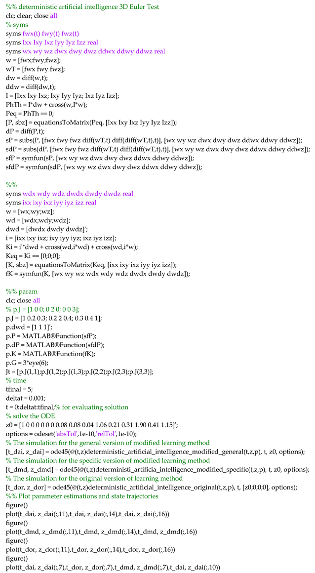
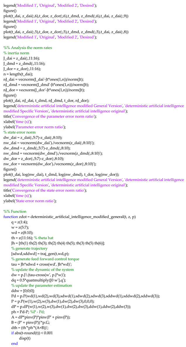
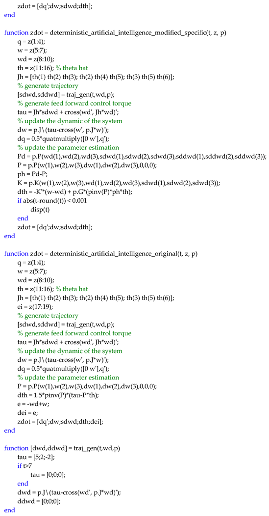
The MATLAB® code used in this manuscript is pasted below. The program utilizes the ode45 solver to simulate the response of the overall system combining the controller and the controlled system.

References

Bucchioni, G.; Innocenti, M. Rendezvous in Cis-Lunar Space near Rectilinear Halo Orbit: Dynamics and Control Issues. Aerospace 2021, 8, 68. [Google Scholar] [CrossRef]
Johnson, M. Space Station Robotic Arms Have a Long Reach. Available online: https://www.nasa.gov/mission_pages/station/research/news/b4h-3rd/hh-robotic-arms-reach (accessed on 23 December 2022).
Mahoney, E. NASA Seeks Ideas for Commercial Uses of Gateway. Available online: https://www.nasa.gov/feature/nasa-seeks-ideas-for-commercial-uses-of-gateway (accessed on 23 December 2022).
NASA Image Use Policy. Available online: https://gpm.nasa.gov/image-use-policy (accessed on 23 December 2022).
Bando, M.; Namati, H.; Akiyama, Y.; Hokamoto, S. Formation flying along libration point orbits using chattering attenuation sliding mode control. Front. Space Technol. 2022, 3, 919932. [Google Scholar] [CrossRef]
Colombia, F.; Colagrossi, A.; Lavagna, M. Characterization of 6DOF natural and controlled relative dynamics in cislunar space. Acta Astronautica 2022, 196, 369–379. [Google Scholar] [CrossRef]
Sands, T. Flattening the Curve of Flexible Space Robotics. Appl. Sci. 2022, 12, 2992. [Google Scholar] [CrossRef]
Sands, T. Optimization Provenance of Whiplash Compensation for Flexible Space Robotics. Aerospace 2019, 6, 93. [Google Scholar] [CrossRef]
Jones, A. Chinese space station robot arm tests bring amazing views from orbit. Available online: https://www.space.com/china-space-station-wentian-robot-arm-test (accessed on 23 December 2022).
Jones, A. See a large robotic arm 'crawl' across China's space station. Available online: https://www.space.com/china-space-station-robot-arm-video (accessed on 23 December 2022).
Zhang, K.; Pan, B. Control design of spacecraft autonomous rendezvous using nonlinear models with uncertainty. J. ZheJiang Univ. 2022, 56, 833–842. [Google Scholar]
Smeresky, B.; Rizzo, A.; Sands, T. Optimal Learning and Self-Awareness Versus PDI. Algorithms 2020, 13, 23. [Google Scholar] [CrossRef]
Slotine, J.; Li, W. Applied Nonlinear Control; Prentice-Hall, Inc.: Englewood Cliffs, NJ, USA, 1991; pp. 392–436. [Google Scholar]
Sands, T. Development of Deterministic Artificial Intelligence for Unmanned Underwater Vehicles (UUV). J. Mar. Sci. Eng. 2020, 8, 578. [Google Scholar] [CrossRef]
Sandberg, A.; Sands, T. Autonomous Trajectory Generation Algorithms for Spacecraft Slew Maneuvers. Aerospace 2022, 9, 135. [Google Scholar] [CrossRef]
Raigoza, K.; Sands, T. Autonomous Trajectory Generation Comparison for De-Orbiting with Multiple Collision Avoidance. Sensors 2022, 22, 7066. [Google Scholar] [CrossRef] [PubMed]
Wilt, E.; Sands, T. Microsatellite Uncertainty Control Using Deterministic Artificial Intelligence. Sensors 2022, 22, 8723. [Google Scholar] [CrossRef] [PubMed]

Figure 1. (a) The International Space Station's Canadarm2 and Dextre carry the Rapidscat instrument assembly after removing it from the trunk of the SpaceX Dragon cargo ship (upper right), which is docked to the nadir port of the Harmony node. (b) NASA Gateway would support a growing space economy Photos taken from [2] and [3] respectively in compliance with NASA’s image use policy [4].

Figure 2. The convergence of the parameter error and state error. (a) Parameter error norm ratio on the ordinant versus time in seconds on the abscissa. (b) State error norm ratio on the ordinant versus time in seconds on the abscissa.

Figure 3. The convergence of the parameter error and state error. Original deterministic artificial intelligence displayed by a thick, solid green line, dashed purple line displays

r = 0.5

, thin solid black line displays

r = 1

, dotted blue line displays

r = 2

, dot-dashed red line displays

r = 4

, (a) Parameter error norm ratio on the ordinant versus time in seconds on the abscissa. (b) State error norm ratio on the ordinant versus time in seconds on the abscissa.

Figure 3. The convergence of the parameter error and state error. Original deterministic artificial intelligence displayed by a thick, solid green line, dashed purple line displays

r = 0.5

, thin solid black line displays

r = 1

, dotted blue line displays

r = 2

, dot-dashed red line displays

r = 4

, (a) Parameter error norm ratio on the ordinant versus time in seconds on the abscissa. (b) State error norm ratio on the ordinant versus time in seconds on the abscissa.

Table 1. Initial condition for the simulation in section 3.1.

Variable	Value	Variable	Value	Variable	Value
$I_{x x}$	1	$I_{y y}$	2	$I_{z z}$	3
$I_{x y}$	0.2	$I_{x z}$	0.3	$I_{y z}$	0.4
$ω_{i n i t, x}$	0.02	$ω_{i n i t, y}$	0.03	$ω_{i n i t, z}$	0.01
$τ_{t e s t, x}$	5	$τ_{t e s t, y}$	2	$τ_{t e s t, z}$	-2
r	3

Table 2. Convergence of inertia estimation and tracking errors.

Figure of merit	Original method (prequels)	Proposed version general	Proposed versionspecific
Parameter error mean	0.0019	0.0027	0.0029
Parameter error deviation	0.0032	0.0037	0.0064
Mean tracking error	0.0401	-0.0094	-0.00037
Tracking error deviation	0.1518	0.0138	0.0065

Table 3. Initial condition for the simulation in section 3.2.

Variable	Value	Variable	Value	Variable	Value
$I_{x x}$	1	$I_{y y}$	2	$I_{z z}$	1
$I_{x y}$	0.2	$I_{x z}$	0.3	$I_{y z}$	0.4
${\hat{I}}_{x x, i n i t}$	1.06	${\hat{I}}_{y y, i n i t}$	1.90	${\hat{I}}_{z z, i n i t}$	1.15
${\hat{I}}_{x y, i n i t}$	0.21	${\hat{I}}_{x z, i n i t}$	0.31	${\hat{I}}_{y z, i n i t}$	0.41
$ω_{i n i t, x}$	0.02	$ω_{i n i t, y}$	0.03	$ω_{i n i t, z}$	0.01
$τ_{t e s t, x}$	5	$τ_{t e s t, y}$	2	$τ_{t e s t, z}$	-2
r	3

Table 4. Convergence of inertia estimation and tracking errors.

Figure of merit	Original method (prequels)	Modified with r = 0.5	Modified with r = 1	Modified with r = 2	Modified with r = 4
Parameter error mean	0.0247	0.0351	0.0348	0.0345	0.0341
Parameter error deviation	0.0124	0.0306	0.0272	0.0239	0.0217
Mean tracking error	-0.0401	-0.0033	-0.0033	-0.0033	-0.0034
Tracking error deviation	0.1761	0.0296	0.0246	0.0189	0.0143

Disclaimer/Publisher’s Note: The statements, opinions and data contained in all publications are solely those of the individual author(s) and contributor(s) and not of MDPI and/or the editor(s). MDPI and/or the editor(s) disclaim responsibility for any injury to people or property resulting from any ideas, methods, instructions or products referred to in the content.

© 2023 by the authors. Licensee MDPI, Basel, Switzerland. This article is an open access article distributed under the terms and conditions of the Creative Commons Attribution (CC BY) license (http://creativecommons.org/licenses/by/4.0/).

Copyright: This open access article is published under a Creative Commons CC BY 4.0 license, which permit the free download, distribution, and reuse, provided that the author and preprint are cited in any reuse.

MDPI Initiatives

Important Links

Choose an area of interest and we will send you notifications of new preprints at your preferred frequency.

Disclaimer

Novel Learning for Control of Nonlinear Spacecraft Dynamics

Abstract

1. Introduction

2. Materials and Methods

2.1. Spacecraft Rotation Rate Control

2.2. Original deterministic artificial intelligence control

2.3. Modified Learning Method, a General Version

2.4. Modified Learning Method, a Specific Version

2.5. Simulation

3. Results

3.1. Performance Comparison without the Product of Inertia

3.2. Performance Comparison with the Product of Inertia

3.3. Performance Comparison with Different r value

4. Discussion

4.1. Recommended Future Work

Conflicts of Interest

Appendix A

References

MDPI Initiatives

Important Links

Subscribe