Prognosease: A Data Generator for Health Deterioration Prognosis

Preprint

Data Descriptor

Prognosease: A Data Generator for Health Deterioration Prognosis

This version is not peer-reviewed.

This version is not peer-reviewed.

Altmetrics

Downloads

159

Views

Comments

Submitted:

25 January 2023

Posted:

26 January 2023

You are already at the latest version

A peer-reviewed article of this preprint also exists.

Abstract

This paper presents PrognosEase; a software that provides an easier way to produce different types of run-to-failure data mimicking real-world conditions to simplify prognosis studies in terms of data collection and improvement in ML degradation modelling process. Different types of degradation types made available to meet different types of applications. Besides, some primary ML tests were performed to ensure that complexity patterns of real systems could be observed in the training/testing predictions attitude. This paper also presents the impacts, limitations and potential improvements of the data generator.

Keywords:

Subject:

Computer Science and Mathematics - Applied Mathematics

This preprints belongs to the Topic

Development of Monitoring, Analysis and Maintenance Technics of Infrastructures

Metadata

Nr	Code metadata description	Please fill in this column
C1	Current code version	v1.0.0
C2	Permanent link to code/repository used for this code version	https://www.mathworks.com/matlabcentral/fileexchange/119743-prognosease
C3	Permanent link to reproducible capsule	none
C4	Legal code license	Batna 2 university
C5	Code versioning system used	none
C6	Software code languages, tools and services used	MATLAB
C7	Compilation requirements, operating environments and dependencies	MATLAB ≥ r2018b
C8	If available, link to developer documentation/manual	none
C9	Support email for questions	berghouttarek@gmail.com

1. Motivation and Significance

Prognosis and health management (PHM) is a discipline dedicated to study health deteriorations of systems under operating conditions [1,2]. Thus, it plays a crucial role in scheduling Condition-Based Maintenance (CBM) tasks while reducing downtime through early failure detection. Remaining Useful Life (RUL) is the primary health indicator, upon which the prognosis process depends to assess the spread of damage during system operating conditions. Indeed, this is the time between the current state of health (SoH) (i.e. the health state prediction time) and the time when the failure could occur. Logically, the run-to-failure RUL labels are obtained from real degradation cycles. However, for some systems (e.g. aircraft engines) it is impossible to achieve such conditions as a higher level of criticality and damage could be achieved, including financial, reputational loss and of life [3].

As an alternative, accelerated aging experiments and simulation models are the available data source used to build data-driven methods [3,4,5]. In this case, acceleration and simulation will not maintain RUL synchronization as in real conditions. Accordingly, other health indicators such as Health Index (HI) and Health Stage (HS) should be used to identify SoH of the system [1,2]. The HI index whose deterioration function is declined in different trends (e.g. linear and exponential) gives information on the current performance of the system. HS indicates the health level of the system at the time of SoH assessment based on some specific divisions (e.g. healthy, critical, and unhealthy SoH) defined by ML developers. Data obtained from accelerated tests suffers from missing patterns and labels, and also suffers from higher-level non-stationarity due to the harsh conditions imposed by the experiment [6]. Moreover, simulation models lack real data patterns. In addition to lacking authenticity at some point, the most significant drawback of both data collection methods is the cumbersome timelines and financial costs that make replication difficult to do.

In this context, it is important to provide an easy way to collect massive data needed to produce and study ML algorithms faster and more accurately as easily as possible. Accordingly, PrognosEase is introduced in this article with the aim of overcoming the shortcomings of accelerated aging and simulation models, simplifying ML studies and speeding up data generation process. The philosophy of PrognosEase depends on the generation of complete life cycles based on specific measurement types and the corresponding HI. These measurements are equivalent to sensor measurements in real applications and show a variety of trends, for example, linear degradation trends like in fuel cells [7], exponential like in turbofan engines [8,9], sinusoidal with exponential growth as in bearings [10], cyclic linear degradation trends as for Li-ion batteries [11]. Since the signals are generated according to some specific patterns, hence they lack RUL timings. In this case, HI and HS can be used. HI from PrognosEase comes with two different types, namely exponential and linear deterioration trends. Non-stationary and changing working conditions are generated as noise and distortion in a kind of randomly injected pulses in the generated measurements. Accordingly, this article is dedicated to presenting all these signals in relation to sensor and HI measurements. Also, it is dedicated to presenting some ML experiments indicating the training attitude and providing similar conclusions to accelerated aging and simulation experiments. In addition, it presents the impact of PrognosEase in the field of PHM, the limitations and potential improvements.

This paper is organized as follows. Besides, the introduction in section 1, section 2 describes PrognosEase and its main features. Section 3 is devoted to some ML experiments conducted using data generated by PrognosEase. Section 4 is devoted to the study of the impact of PrognosEase in the field of PHM. Section 5 presents limitations and potential improvements. Finally, Section 5 concludes this work.

2. Software Description

This section is dedicated to introducing different aforementioned types of measurements in life cycles generated by PrognosEase in two different subsections, both sensor measurements generation and also types of HI trends.

2.1. Generating Sensors Measurements

As mentioned earlier, the measurement trends are generated according to some specific variations inspired by some well-known works in the literature, including linear, exponential and exponentially growing sinusoidal, cyclic with linear and exponential trends. Additional features such as noise and distortions have been added to emulate real-world conditions affecting the system.

Linear: The sensors measurement describing a linear trend

L

are generated according to a linearly growing function with the slop

a

and initial value

b

for an input time unites

x

as in one (1). A random noise

μ

is generated from a specific type of probability distribution

P (x)

defined according to user experience as addressed by (2). After that, the noise

μ

and the degradation trend

L

are summed up while the noise is penalized with some specific noise rate

ϑ

to construct the signal

S_{N}^{*}

as in (3). Next,

S_{N}^{*}

will be scaled in range

[0,1]

using min-max normalization as in (4) to obtain

S_{L}^{* *}

. Finally,

S_{L}^{* *}

will subject to some random distortion

ρ

with random number of pulses

n ρ

controlled according specific amplitude

w

, and normalization factors

{α_{ρ}, β_{ρ}}

, to generate the final measurements

S_{L}

as in (6) while, the pulses are periodically generated according to the discreet function as in (5).

L = a x + b

(1)

μ = P (x)

(2)

S_{N}^{*} = (ϑ L) μ + L

(3)

S_{N}^{* *} = \frac{S_{N}^{*} - m i n (S_{N}^{*})}{\max (S_{N}^{*}) - m i n (S_{N}^{*})}

(4)

ρ = {w e^{\pm \ln (α_{ρ}) x (i) / β_{ρ}}}_{i = 1}^{n ρ}

(5)

S_{L} = S_{N}^{* *} + ρ^{L}

(6)

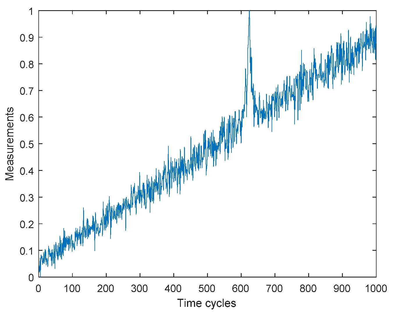
Figure 1 showcases an example constructing a linear sensors measurement trend with

P (x)

is a Gaussian noise,

ϑ = 0.9

n ρ = 2

w = 0.1

Exponential: Sensors measurements describing an exponential trend

E

are generated according to Formula (7) with the base of exponentiation

e

and exponentiation parameter

α_{E}

. The measurements of

E

follows similar steps of corruptions by adding the noise and distortions pulses while, scaling is also necessary (i.e. Equations (3)–(5)) to finally attend the

S_{E}

as in (8).

E = e^{(α_{E} x)}

(7)

{S_{E} = S}_{N}^{* *} + ρ

(8)

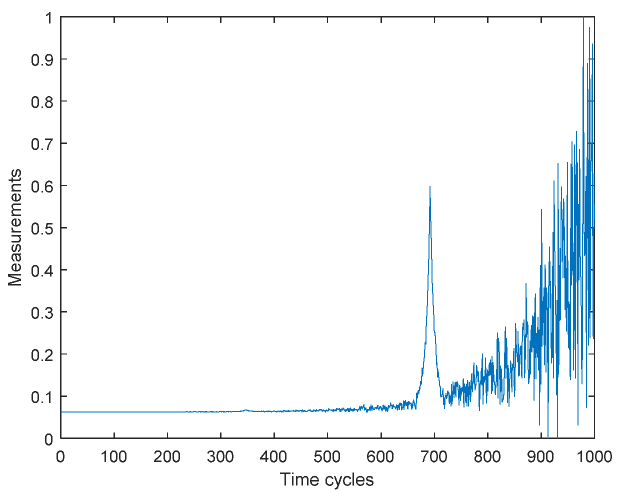
Figure 2 is an example constructing a sensor measurements according to an exponential trend with

P (x)

is a Gaussian noise,

ϑ = 0.03

n ρ = 2

w = 0.1

. and

α_{E} = 0.01

Sinusoidal with exponential growth: This type of measurements of sinusoidal with exponential growth

S E

are generated according to Formula (9) with an exponentiation parameter

α_{S E}

and angular frequency

ω

while being subject to distortion by noise and randomly injected pulses until the final shape

S_{S E}

reached using Formula (10).

S E = e^{(α_{S E} x)} c o s (ω x)

(9)

{S_{S E} = S}_{N}^{* *} + ρ

(10)

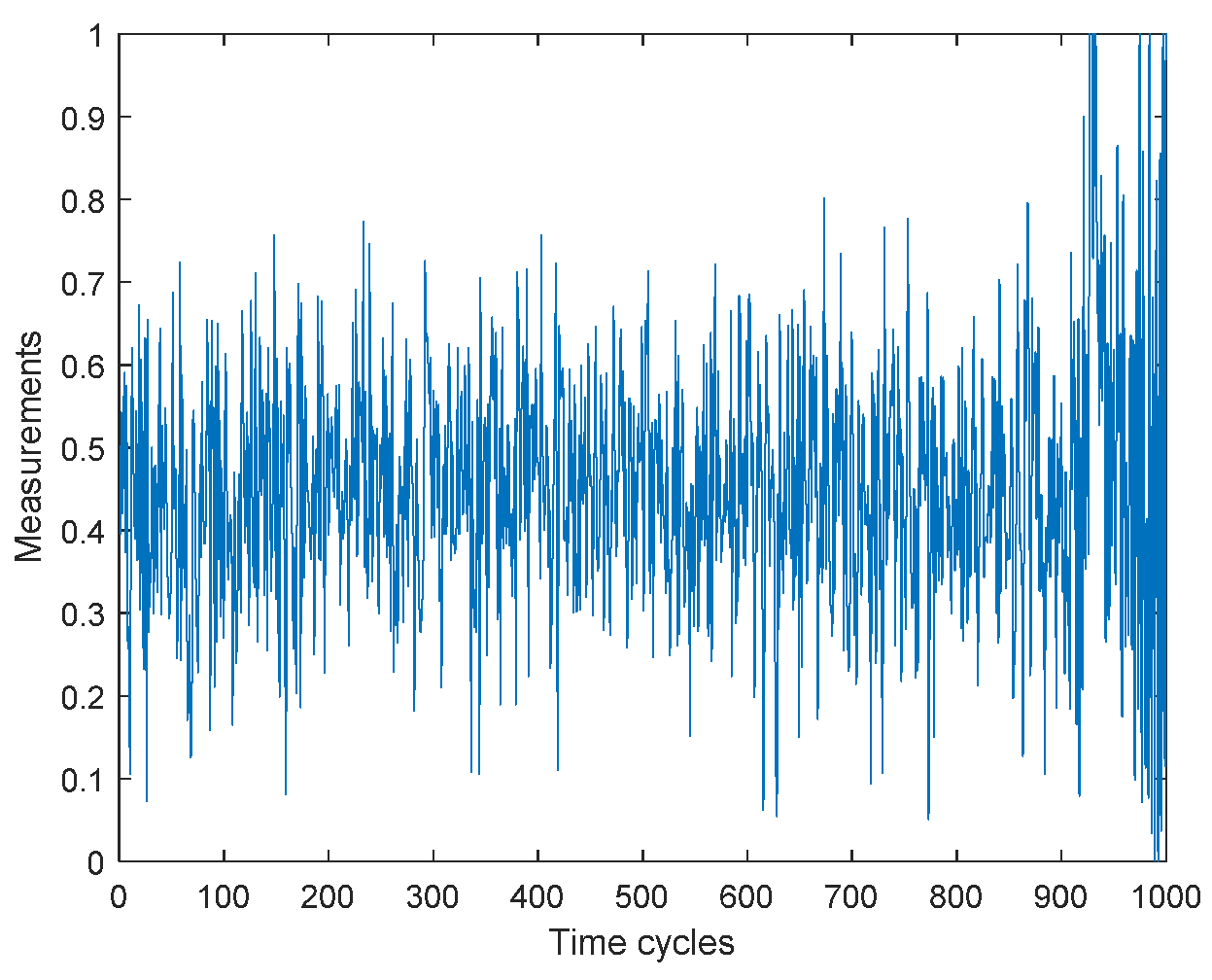
Figure 3 is an example constructing a sensor measurements according to a sinusoidal with exponential growth trend with

P (x)

is a Gaussian noise,

ϑ = 0.1

n ρ = 2

w = 0.1

α_{S E} = 0.02

, and

ω = 0.2

Cyclic degradation: The cyclic degradation

S_{C}

comes up with two types (i.e. linear and exponential trends). The pulses are similarly generated according to Equation (5) but periodically with a distance between pulses

D

dynamically changes at each cycle with a specific user ratio

ϑ_{C}

as in Formula (11) while (12) is describing the final output signal.

ρ = {w e^{\frac{\pm \ln (α_{ρ}) x (i)}{β_{ρ}}} + {ϑ_{C} D}}_{i = 1}^{n ρ}

(11)

{S_{C} = S}_{N}^{* *} + ρ

(12)

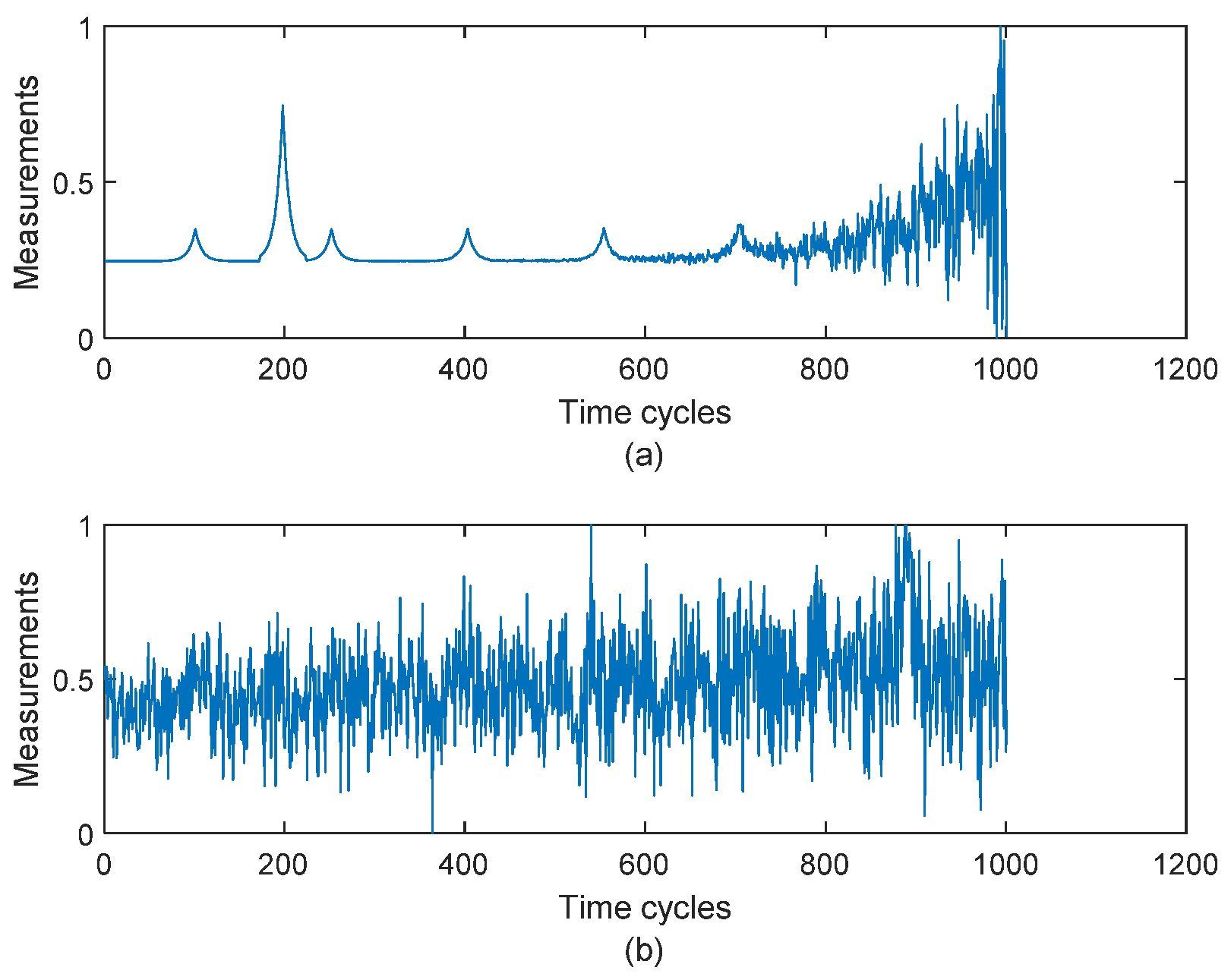
Figure 4 is an example that showcases both types of cyclic degradation that PrognosEase programed to do.

2.2. Generating RUL Measurements

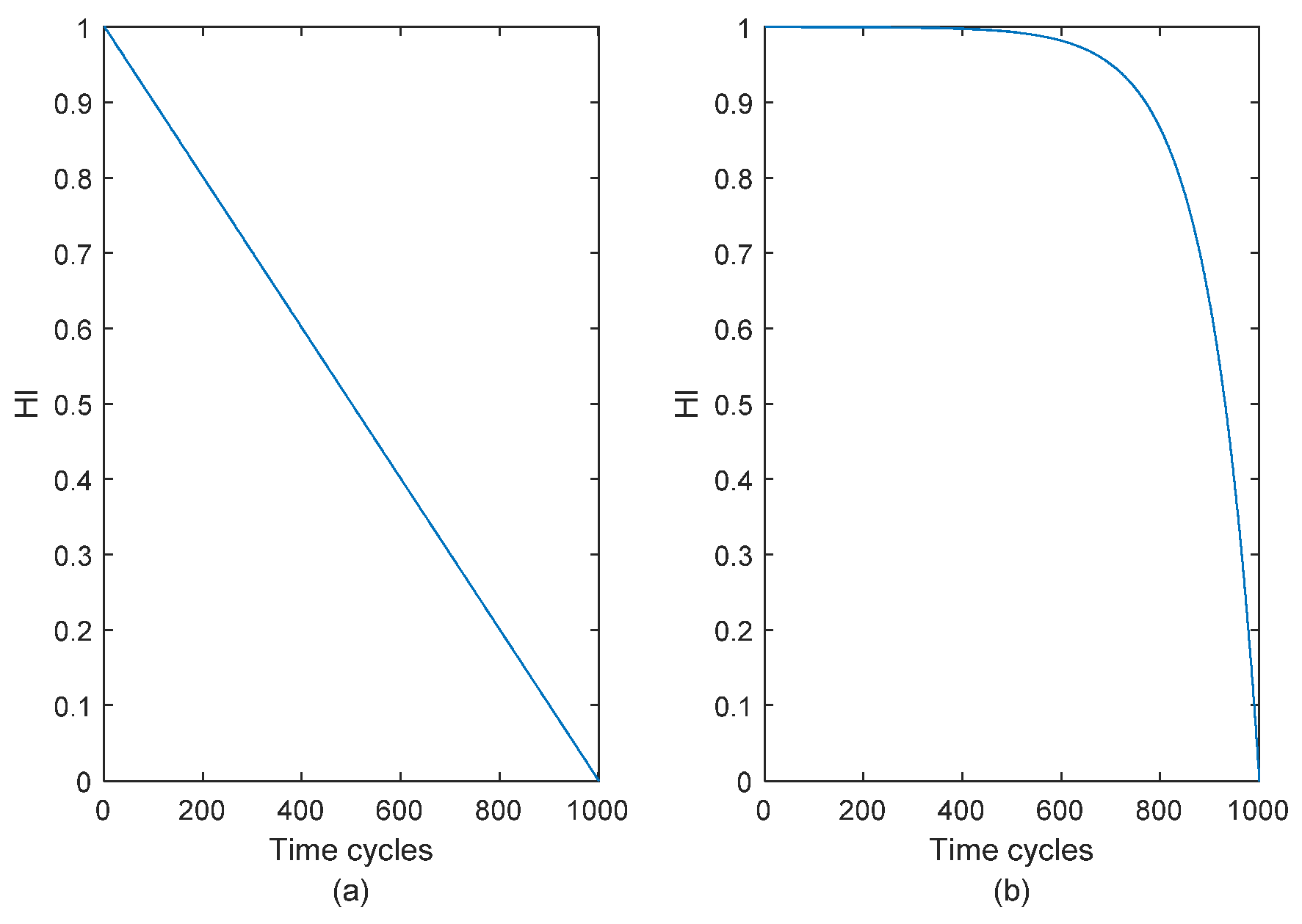
In PrognosEase, RUL degradation function is actually a HI generated according to two main trends either exponential or linear following Formulas (1) and (7) respectively with different parameters values from the sensors measurements. These parameters are user-defined ones depends on accuracy of predictions and also user experience. The example in Figure 5 illustrates both types of HIs.

3. Illustrative Examples

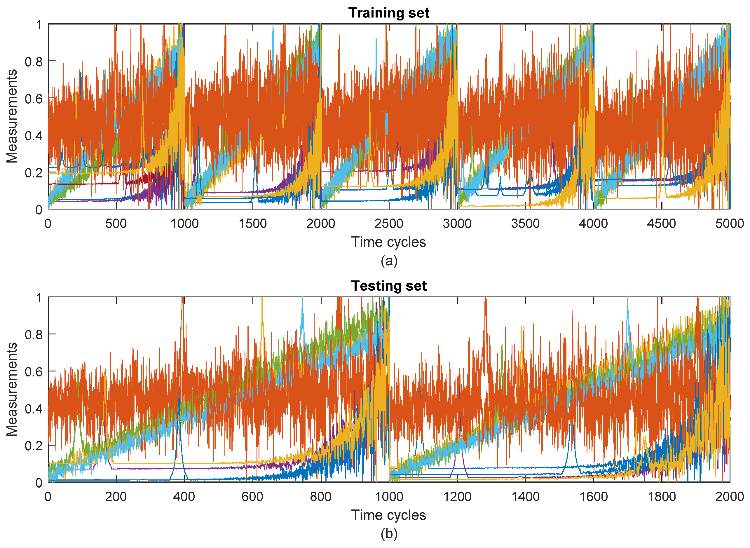
In this study, PrognosEase is used to generate a dataset that combines a mixture of sensor measurements types with a higher level of complexity, similar to the work done in the literature in terms of data generation. 10 features, 5 lifecycles for training and 2 cycles for testing are generated with cycles that are 1000 samples long. The training and testing lifecycles are showcased in Figure 6. The data visualization addresses that the constructed features space includes different types of complex samples with higher-level non-stationarity. In fact, these samples are supposed to be flown from the same devices under different conditions. This means that all data generation parameters are fixed when reconstructing the data set while retaining only the noise generation and distortion that changes the conditions. This is done with the aim of reaching a certain level by mimicking real-world conditions. HI is set in this case by default to the exponential deterioration function due to the existence of an exponential deterioration phenomenon in the collected measurements.

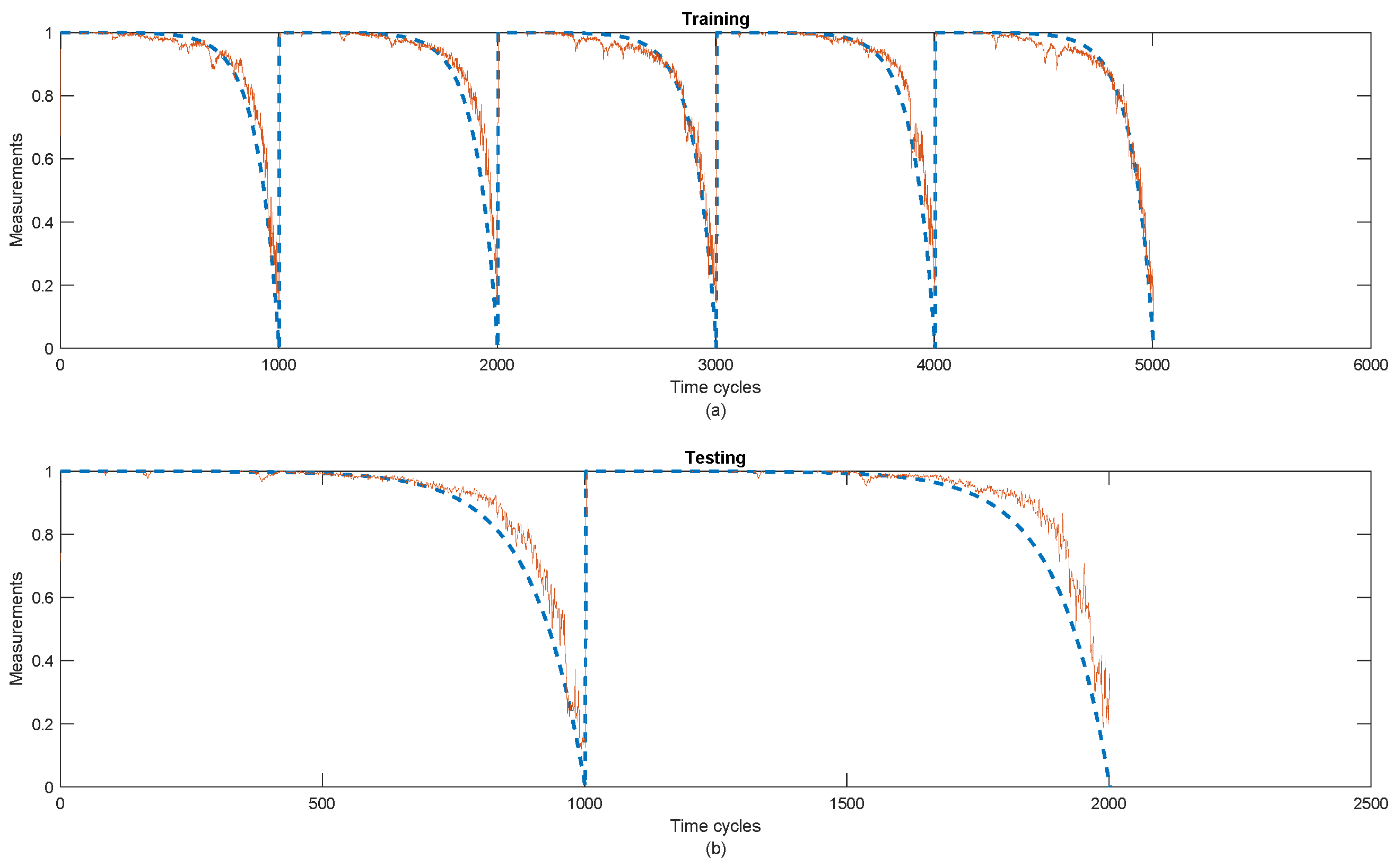
An ML model, namely a long-term memory neural network, is tested for its potential capabilities using a grid search mechanism to adjust its parameters for a better approximation. The curve fitting results for training and testing are shown in Figure 7. The learning model shows that it tries to mimic the shape of the decay trend in the training process as it is logically difficult to do for new unseen samples to the model. Thus, improving ML models will consist of improving the curve fitting as much as possible in the testing phase while taking into account real-world conditions and training constraints such as centralized, decentralized and federated learning, etc., with all types of learning paradigms such as online, offline and reinforcement learning etc.

4. Impact

PrognosEase actually introduced an effective and a simple way to study ML models for deterioration analysis. Its simplicity remains in following items:

Easily generating many types of degradation samples with any preferred number of training and testing cycles making useful for many types of many applications.
PrognosEase simplifies centralized learning for both offline and online learning.
PrognosEase also allows experiments to be done according decentralized and federated learning [12].
PrognosEase provides a feature space accessing times series experiments for both cyclic and non-cyclic degradation.
PrognosEase provides features achieving great experiments on direct HI predictions experiments.
PrognosEase doesn’t follow supervised direct HI and time series predictions; in fact, it can be used for unsupervised HS assessment with clustering methods also.
PrognosEase allows experiments not only be limited to improving ML methods. In fact, it can also be used for studying data quality and preprocessing tools also.

5. Limits and Potential Improvements

PrognosEase has limits in addressing reality in context of following items:

Similar to simulation and accelerated aging, PrognosEase doesn’t have the capability of estimating actual RUL timing. Rather than that, it provides His instead.
PrognosEase comes up with Gaussian noise only, so potential improvement will consist of adding more types of noises to approach reality when emulating real conditions.
Only single type of pulses generation when distorting generated measurements. Accordingly, more efforts can be made on generating other pulses types mimicking distortions in real applications.
For cyclic degradations better formulas could be released to better control cycles dynamic changes as in real systems such as for batteries for instance.

6. Conclusions

This paper presented PrognosEase; a software for generating run-to-failure data for Data-driven prognosis studies. PrognosEase mimics real conditions of different systems by generating similar measurements to their real degradation trends and working conditions. Data visualization for feature spaces generated by PrognosEase and Some ML experiments shows that the software is able to address prediction complexity for unseen samples as in real samples. This paper also presented impact of PrognosEase in PHM filed besides to some future prospects on its potential improvements.

References

Berghout, T.; Benbouzid, M. A Systematic Guide for Predicting Remaining Useful Life with Machine Learning. Electronics 2022, 11, 1125. [Google Scholar] [CrossRef]
Lei, Y.; Li, N.; Guo, L.; Li, N.; Yan, T.; Lin, J. . Machinery health prognostics: A systematic review from data acquisition to RUL prediction. Mech. Syst. Signal Process. 2018, 104, 799–834. [Google Scholar] [CrossRef]
Saxena, A.; Goebel, K.; Simon, D.; Eklund, N. Damage propagation modeling for aircraft engine run-to-failure simulation. in 2008 International Conference on Prognostics and Health Management, Oct. 2008, pp. 1–9. [CrossRef]
P. Nectoux et al. PRONOSTIA : An experimental platform for bearings accelerated degradation tests. in IEEE International Conference on Prognostics and Health Management, PHM’12, 2012, pp. 1–8, [Online]. Available: http://hal-obspm.ccsd.cnrs.fr/UNIV-BM/hal-00719503.
Prognostics Center of Excellence. PRONOSTIA-FEMTO Bearing Data Set. 2012. https://ti.arc.nasa.gov/tech/dash/groups/pcoe/prognostic-data-repository/#turbofan.
Berghout, T.; Mouss, L.-H.; Bentrcia, T.; Benbouzid, M. A Semi-Supervised Deep Transfer Learning Approach for Rolling-Element Bearing Remaining Useful Life Prediction. IEEE Trans. Energy Convers. 2022, 37, 1200–1210. [Google Scholar] [CrossRef]
Berghout, T.; Benbouzid, M.; Bentrcia, T.; Amirat, Y.; Mouss, L. Exposing Deep Representations to a Recurrent Expansion with Multiple Repeats for Fuel Cells Time Series Prognosis. Entropy 2022, 24, 1009. [Google Scholar] [CrossRef] [PubMed]
Berghout, T.; Mouss, L.H.; Kadri, O.; Saïdi, L.; Benbouzid, M. Aircraft engines Remaining Useful Life prediction with an adaptive denoising online sequential Extreme Learning Machine. Eng. Appl. Artif. Intell. 2020, 96, 103936. [Google Scholar] [CrossRef]
Berghout, T.; Mouss, L.; Kadri, O.; Saïdi, L.; Benbouzid, M. Aircraft Engines Remaining Useful Life Prediction with an Improved Online Sequential Extreme Learning Machine. Appl. Sci. 2020, 10, 1062. [Google Scholar] [CrossRef]
Berghout, T.; Benbouzid, M.; Mouss, L.H. Leveraging label information in a knowledge-driven approach for rolling-element bearings remaining useful life prediction. Energies 2021, 14, 2163. [Google Scholar] [CrossRef]
Saha, B.; Goebel, K. Saha, B.; Goebel, K. Battery data set. NASAAMES Progn. Data Repos. 2007.
Berghout, T.; Bentrcia, T.; Ferrag, M.A.; Benbouzid, M. A Heterogeneous Federated Transfer Learning Approach with Extreme Aggregation and Speed. Mathematics 2022, 10, 3528. [Google Scholar] [CrossRef]

Figure 1. An example of a sensors measurements generated according a linear trend.

Figure 2. An example of a sensors measurements generated according an exponential degradation trend.

Figure 3. An example of a sensors measurements generated according a sinusoidal with exponential growth trend.

Figure 4. An example of a sensors measurements generated according a cyclic degradation trend: (a) An exponential cyclic degradation; (b) A linear cyclic degradation.

Figure 5. An example of HI degradation functions: (a) A linear degradation; (b) An exponential degradation.

Figure 6. Visualizing feature spaces of a dataset generated by Prognosis: (a) Training set; (b) Testing set.

Figure 7. Visualizing Curve fit results with a deep learning network: (a) Training set; (b) Testing set.

Disclaimer/Publisher’s Note: The statements, opinions and data contained in all publications are solely those of the individual author(s) and contributor(s) and not of MDPI and/or the editor(s). MDPI and/or the editor(s) disclaim responsibility for any injury to people or property resulting from any ideas, methods, instructions or products referred to in the content.

© 2023 by the authors. Licensee MDPI, Basel, Switzerland. This article is an open access article distributed under the terms and conditions of the Creative Commons Attribution (CC BY) license (http://creativecommons.org/licenses/by/4.0/).

Copyright: This open access article is published under a Creative Commons CC BY 4.0 license, which permit the free download, distribution, and reuse, provided that the author and preprint are cited in any reuse.

Alerts

MDPI Initiatives

Important Links

Choose an area of interest and we will send you notifications of new preprints at your preferred frequency.

Disclaimer

Prognosease: A Data Generator for Health Deterioration Prognosis

Abstract

Keywords:

Subject:

Metadata

1. Motivation and Significance

2. Software Description

2.1. Generating Sensors Measurements

2.2. Generating RUL Measurements

3. Illustrative Examples

4. Impact

5. Limits and Potential Improvements

6. Conclusions

References

MDPI Initiatives

Important Links

Subscribe