You are currently viewing a beta version of our website. If you spot anything unusual, kindly let us know.

Preprint

Article

Nearest Neighbours Graph Variational AutoEncoder

Altmetrics

Downloads

133

Views

Comments

A peer-reviewed article of this preprint also exists.

Lorenzo Arsini^*

Barbara Caccia,Andrea Ciardiello,

Stefano Giagu^*

Carlo Mancini Terracciano^*

Lorenzo Arsini^*

Barbara Caccia,Andrea Ciardiello,

Stefano Giagu^*

Carlo Mancini Terracciano^*

This version is not peer-reviewed

Abstract

We present a Deep Learning generative model specialized to work with graphs with a regular geometry. It is build on a Variational Autoencoder framework and employs Graph convolutional layers in both encoding and decoding phases. We also introduce a pooling technique (ReNN-Pool), used in the encoder, that allows to downsample graph nodes in a spatially uniform and highly interpretable way. In the decoder, a symmetrical un-pooling technique is used to retrieve the original dimensionality of graphs. Performance of the model are tested on the standard Sprite benchmark dataset, a set of 2D images of video game characters, adequately transforming images data into graphs, and on the more realistic use-case of a dataset of cylindrical-shaped graph data that describe the distributions of the energy deposited by a particle beam in a medium.

Keywords:

Subject: Computer Science and Mathematics - Computer Vision and Graphics

1. Introduction

Deep Generative Modeling consists in the training of a deep neural network to approximate the high dimensional probability distribution of the training data, allowing to generate new examples from that distribution. Image generation has in particular took advantage of Convolutional Neural Networks (CNN) [1,2,3] layers, now recognized as one of the most powerful tool to process grid-like data in Deep Learning frameworks. Different approaches to deep generative modeling exist [4], as for example Generative Adversarial Networks (GAN) [5], Variational AutoEncoders (VAE) [6], Energy based models [7], Normalizing Flow models [8], and Diffusion models [9]. In some cases, architectures include both an encoding and a decoding scheme. This is the case for architectures as Variational AutoEncoders. The encoding is usually done to obtain compact representations of data distribution and is often carried out using pooling operations that allow to reduce the dimensionality of data. Embedding the input samples in lower and lower dimensional spaces creates a so called "bottle-neck" in the process, thanks to which essential features of data can be extracted. The decoding scheme, on the other hand, often employs reverse operations used in the encoding, such as Transpose Convolutions and un-pooling operations.

While CNNs are powerful tools to handle grid-like data, a lot of interesting real-world phenomena are described by data with a strong irregular structure and a richness in relation information among elements. Typical tasks with such datasets regard modeling physical systems, studying protein structure or understanding people’s working and social networks. To deal with such learning tasks, whose related data can be generally arranged in a graph structure, there is an increasing interest in Graph Neural Networks (GNN). Such architectures use, in most cases, Graph Convolutional layers (GCN), which allow to process data on graph generalizing the idea of convolutions in CNNs. There are currently several types of GCNs, from the simplest models [10,11], to those based on graphs’ spectral properties [12] or that add mechanisms of attention [13]. While is currently possible to solve different problems of classification, regression or link prediction on graphs with excellent results, graph generation is still a tough challenge [14]. In particular, defining pooling and un-pooling operations on graph structure, which would allow the possibility to create bottle-necks in architectures, is not trivial. Moreover, while some ways to embed graph data in low dimensional representations have been developed [15], there is still a considerable lack of decoding solutions that take into account the graph structure of data and employ graph convolutional layers.

In this context, we propose a model for graph generation based on Variational Autoencoders. We limit ourselves to the case of graph data with a fixed, regular and known geometrical structure. With this constraint, we are able to build a model where both encoding and decoding are done using Graph convolutional layers. To create a bottle-neck we also employ novel symmetrical pooling and un-pooling operations fully taking advantage of known graphs’ geometry.

1.1. Related Works

In this section we present relevant works related to Variational Autoencoders, Graph Convolutional layers, pooling and un-pooling operations on graphs.

1.1.1. Variational AutoEncoder

A Variational Autoencoder is a generative Deep Learning model first proposed by Kingma and Welling [6]. It is a special autoencoder based on variational Bayes inference whose goal is to learn the distribution of the training data and to be able to sample new datapoints from it. The underlying hypothesis is that datapoints

{x}

are the results of a generative process controlled by a variable z that lives in a low dimensional space, called latent space, and their distribution is thus:

p (x) = \int p (x | z) p (z) d z,

where the prior

p (z)

is often considered Gaussian. The model is made up of two networks: the encoder and the decoder. The encoder

q_{ψ} (z | x)

maps the input data to a distribution in the latent space. Thanks to the reparemeterisation trick, a point from such distribution is sampled in a fully differentiable way and processed by the decoder

p_{ψ} (x | z)

to retrieve the original data. The model is trained maximising the evidence lower bound (ELBO) of the data likelihood:

{ψ, ϕ} = a r g m a x_{ψ, ϕ} [E_{x \sim q_{ψ} (\cdot | x)} [l o g p_{ϕ} (x | z) - D_{K L} (q_{ψ} (z | x) | p (z))]]

After training, new datapoints x can be generated sampling z in the latent space and passing it to the decoder. Starting from a standard VAE, it is also possible to slightly modify the loss function adding a scalar hyperparameter

β > 1

{ψ, ϕ} = a r g m a x_{ψ, ϕ} [E_{x \sim q_{ψ} (\cdot | x)} [l o g p_{ϕ} (x | z) - β D_{K L} (q_{ψ} (z | x) | p (z))]] .

The model with such modification is known as

β -

VAE [16] and is recognised to promote a better disentangling of features’ embedding in the latent space.

1.1.2. Graph generation

Graph generation is, in general, a hard task. Unlike images, graphs often have complex geometrical structure that are difficult to reproduce, especially in an encoder-decoder framework. Though different approaches exist, there is yet no standard method to address such class of problems. Standard classes of models for graph generation are GAEs and VGAEs [17] which bring the idea of autoencoders and VAEs on graph. However these architectures reconstruct or generate only the adjacency matrix of the graphs and not their nodes’ features. Moreover, while is it true that such models can learn meaningful embeddings of nodes features, in the encoding process the graph structure and the number of nodes remains fixed. There is therefore no real compression of input data by pooling operations and no bottle-neck at all.

Regarding pooling operations on graphs, different strategies have been developed. Early works use eigen-decomposition for graph coarsening operations based on graphs’ topological structure. However, these methods are often time consuming. A popular algorithm which is alternative to eigen-decomposition approaches is Graculus [18], used in [12] and later adopted in other works on GNNs. Other different approaches select nodes to pool accordingly to their importance in the Network, as in the case of SortPooling [19]. There is also a stream of literature that bases pooling operation on spectral theory [20,21]. Finally, state of art approaches rely on learnable operators that, like message-passing layers, can adapt to a specific task to compute optimal pooling. Examples of this are DiffPool [22] and Top-K pooling [23].

While there are different solutions in current literature for pooling procedure, the same is not true for un-pooling operation. In general, there is no obvious way to define a un-pooling procedure for graphs that can be thought as the inverse operation of pooling. The only works that try to define such operation are described in [24] and [23]. Other decoding scheme for graph generation are thought in different ways that, in most cases are task specific. For example in many algorithms for protein or drugs structure generation the decoding is done adding nodes and edges sequentially [25,26]. On the other hand, there are also works on "one-shot" graph generation, with decoding architectures that can output nodes’ and edges’ features in a single step [27,28]. However, in various works that use this approach, the decoding of nodes and edges is considered separately and does not take into account the structure of graphs. For example in [29] a 1D-CNN is used to decode the node features and a 2D-CNN for the edge features.

In the end, in literature there is no unique and established way to address the problem of graph generation. In this etherogeneous context our main contribution are:

simple, symmetrical and geometry-based pooling and unpooling operations;
a Varational AutoEncoder for regular graph data where both encoding and decoding modules employ graph convolutional layers.

2. Materials and Methods

2.1. Nearest Neighbour Graph VAE

In this section, we introduce our Graph VAE model that uses Graph convolutions both in encoding and decoding operation. To create a bottle-neck in the encoding, we also propose a new graph pooling technique, to which we will refer as Recursive Nearest Neighbour Pooling (ReNN-Pool). Introducing such pooling technique allows us also to define a symmetrical un-pooling operation that we use to build a VAE’s decoder based on graph convolutions.

2.1.1. ReNN-Pool and Un-Pool

In CNNs, on grid-like data, pooling operations are widely used to decrease the dimensionality of feature maps while increasing neurons’ receptive fields. On images, for example, a standard pooling layer consists in a downsampling operation, like the max or the mean function, applied to sets of nearby pixels. For grid-like data, this is easily possible because of their simple and known geometry. Bringing this idea to graph structures is, in general, a hard task. However, there are cases in which, although data don’t have a grid-like shape and so can be better processed with GNNs, the graphs structures are fixed and have a regular and known geometry. For example, some datasets can contain examples whose data is arranged in a cylindrical or spherical structure. For this cases, we developed a simple pooling operation (ReNN-Pool) that can sub-sample graph nodes in a regular way. In its basic application, it consists in a masking operation and a subsequent change in the adjacency matrix of the graph. The masking operation is performed dividing the nodes in two sets: nodes in the first set are kept, while the others are dropped. These two sets are built recursively. First, nodes are sorted on the basis of their position in the graph. For example, if samples have a cylindrical structure, nodes can be hierarchically ordered on the basis of their positions along the z,

θ

and r axes. After the ordering, the process starts from a node. That node is kept, while all its nearest neighbours nodes are dropped, removing them from the nodes’ list. The process, then, repeats moving on the whole node list. After the masking we rewire links between the "survived" nodes, connecting to each other the ones that were 2^nd nearest neighbours before the masking. In practice, we are changing the adjacency matrix from A to

A^{2}

. We specify that all the adjacency matrices are intended to be binary: element

a_{i j}

is 1 if a link between

i - t h

and

j - t h

node exists and 0 otherwise. So, even after the adjacency augmentation from A to

A^{2}

, the new matrix is binarised. If we call M the vector that contains all the indices of the "surviving" nodes,

X = {x_{i}}_{i = 1}^{N}

and A respectively the nodes’ feature matrix and the adjacency matrix before the pooling, the application of ReNN-Pool gives in output:

\begin{matrix} X^{'} = {x_{i}^{'}}_{i = 1}^{N}, where x_{i}^{'} = \{\begin{matrix} x_{i}, & if i \in M \\ 0, & otherwise \end{matrix} & A^{'} = \{\begin{matrix} A_{i j}^{2}, & if i, j \in M \\ 0, & otherwise \end{matrix} \end{matrix}

The process is illustrated in Figure 1

In case of regular geometrical graph structures, the choice of the starting node should not affect the performances of the model in which the ReNN-Pool is used. In fact, by construction, pooled and not-pooled nodes are evenly spread across the whole graph. For irregular graph structure, performance can depend on the choice of the first node. However, in principle this can become an hyperparameter to optimize using a validation set. Such possibility will be explored in a future work.

Moreover, to emulate classical pooling in CNNs, one can also add a function to the simple masking operation. Instead of just keeping a node as it is and dropping its nearest neighbour, one can sum or concatenate its features with the max (or the mean) of the features of the neighbours nodes.

Due to the fact that the creation of masks and the adjacency matrices’ augmentation in our pooling only depends on the graph structure of data, it is possible to compute and store them before the training. Such masks and adjacencies can also be used to define an un-pooling operation that is symmetrical to the pooling one. A similar idea was already explored [23]. Starting from a lower dimensional (pooled) representation of the graph with feature matrix X and adjacency

A^{2}

, the un-pool layer simply embed back the nodes in their positions in the higher dimensional representation of the graph, that has adjacency matrix A. All other nodes’ features are set to 0. An illustration of the un-pooling operation is shown in Figure 2

2.1.2. ReNN Graph VAE architecture

In our architecture, the encoding consists in three subsequent repetitions of two operations: a graph convolution and a ReNN-Pool operation. For the graph convolution we chose to use the GraphConv layer [10] for its simplicity and direct interpretability. With this convolution, the new features of nodes are just linear combinations between their old features and the mean of the features of their neighbourhood, followed by a ReLu activation:

x_{i}^{'} = R e L u (W_{1} x_{i} + W_{2} \frac{1}{| N (i) |} \sum_{j \in N (i)} x_{j}) .

(1)

Eventually, to increase the expressive power of the network, one can also include edge features

e_{i j}

in the computation considering instead:

x_{i}^{'} = R e L u (W_{1} x_{i} + W_{2} \frac{1}{| N (i) |} \sum_{j \in N (i)} e_{i j} x_{j}) .

(2)

In particular, we consider edge features

e_{i j}

to be independent from the nodes’ features and directly learned through a Linear layer.

We chose the output channels of the GraphConv to increase in the three subsequent repetitions, being 16, 32, and 64 channels, as in standard practice.

After the three graph encoding steps, nodes features are put together and flattened. Then, the dimensionality of data is further reduced through a linear layer.

The encoded data is processed as in standard VAE architecture, using the reparameterisation trick, mapping the input data to Gaussian distributions in the latent space and sampling a variable Z from that distribution.

The decoding uses the same graph representations employed for the encoding, but in reverse order. After an initial decoding linear layer, we repeat for three times the series of an un-pooling layer and a graph convolution. For the convolution, again we employ the GraphConv layer, but in this case the number of channels in the three repetitions decreases: from 64 to 32 to 16. In this way the original dimensionality of the data is recovered. Moreover, the activation function of the last convolutional layer is a sigmoid instead of a ReLu. The model is trained minimizing the standard

β

-VAE loss function, with binary cross entropy as the reconstruction term.

In general, one can think the concatenation of a graph convolution and a pooling operation as an "encoding block" and the union of an un-pooling operation and a convolution as a "decoding block". Various architectures can be then build using different numbers of blocks. In Figure 3, for example, our VAE architecture is illustrated, but with only two blocks in encoder and decoder.

2.2. Datasets

2.2.1. Energy deposition datasets

The architecture presented in this work was developed for a specific application in Medical Physics, which is the generation of the distribution of the dose absorbed by a medium interacting with a given particle beam, conditioned to beams parameters and medium density.

The datasets for this task are built simulating an electron beam interacting with a material using Geant4 [30], a toolkit in C++ for Monte Carlo simulations in particle physics.

The two datasets differ on the material in which electrons deposit their energy. In the first case, this material is just a cubic volume filled with water. We will refer to this dataset as "Water Dataset". In the second case, to increase the complexity of the task, we inserted a slice of variable density in the water volume. This slice is orthogonal to the electrons’ beam and has fixed position and thickness. The density of the slice is uniformly extracted at each run of simulation between 0 and 5

g / c m^{3}

(for reference, water density is 1

g / c m^{3}

) . We will refer to this dataset as "Water + Slice Dataset". In both cases particles’ energies are sampled uniformly between 50 and 100 MeV, which is the typical range of energies of a radiotherapy treatment.

Energy deposition data are collected in a cylindrical scorer, aligned with the electron beam, divided in 28 x 28 x 28 voxels along z,

θ

and r axes. The cylindrical shape is particularly useful in our application because it allows for higher precision near the beamline.

Each example in the dataset is therefore a set of

28^{3}

voxels arranged in a cylindrical shape. Voxels have only one feature, that correspond to the amount of the energy deposited in them by the simulated particle beam. Each example of the Water Dataset is labelled by the initial energy of the electron beam, while in the other dataset examples are labelled by both the particles’ initial energy and the slice’s density.

Both datasets are made up of nearly 5000 examples each and are divided in train, validation and test sets on the basis of particles’ energy and slice’s density. In particular, in the Water Dataset the test set is made up of examples with particle’s energy ranging between 70 and 80

M e V

. In the Water + Slice Dataset test set, examples have the same range of initial energies and slice’s density values ranging between 2 and 3

g / c m^{3}

. In both cases, the rest of the dataset is used for validation and train with a ratio of

1 / 10

Test sets have been chosen in this way in order to test the network ability to interpolate between samples and generalise to unseen configurations.

For both datasets we imposed a graph structure on data. Each voxels was associated with a node and nodes were linked within each other with a nearest neighbours connectivity.

2.2.2. Sprite dataset

The Sprite dataset consist in a set of 2D images representing pixelized video game “sprites”. The aim of testing our Graph VAE on such dataset is to show that our model can also work as a standard Variational AutoEncoder on tasks that are different from the one it was developed for. Although, it is widely reasonable that CNNs would be the beast suitable choice to work with images, these grid-like data can also be thought as graph with a regular structure and so, should be processed in a good way also by our model.

The Sprite dataset comes from an open-source video game project called Liberated Pixel Cup1. Sprite images can also be freely created and downloaded from the authors’ github2. In particular we used part of the dataset employed in [31], available online3. Such dataset consists in 9000 examples for training and 2664 for test. Each example is a sequence of 8 frames of a sprite performing an action. We decided to keep the first frame for each example, so we ended up with 9000 images, divided in training and validation set with

1 / 8

ratio, and 2664 images for test. Each image is

64 x 64

pixels and represents a standing sprite whose attributes are organized in 4 categories (skin color, tops, pants and hairstyle) with 6 variation each, and 3 orientations (left, center and right).

To process such dataset with our architecture, we had to impose a graph structure on data. So, we associated a node to each pixel and connected nodes with a grid-like connectivity. In this way, internal nodes have 4 edges, border nodes have 3 edges and corner nodes 2.

3. Results

3.1. Results on energy deposition datasets

We trained our VAE with the two energy deposition datasets described in the previous section. Here, we present the results that regards the reconstruction of the energy deposition distribution from the test set. The DL model was trained for 200 epochs and the best set of learnable parameters was chosen as the one that minimizes the validation loss. We set the latent space dimensionality to 1, for the Water Volume dataset, and to 2 for the other dataset. For the weight update we used the Adam optimiser with an initial learning rate of 0.003 and an exponential scheduler with

λ = 0.9

. The hyperparameter

β

was set to 1.

To evaluate the performance of our model in sample reconstruction we considered two types of metrics. The first type concerns node-per-node (voxel-per-voxel) reconstruction. Among available node-per-node metrics we chose to use the

δ

index, developed by [32], for its high interpretability. The reconstruction error on each node is thus defined as:

δ = \frac{X_{r e c o} - X_{G T}}{m a x (X_{G T})}

(3)

where

X_{r e c o}

is the node feature predicted by the VAE, while

X_{G T}

is the ground truth node feature in the corresponding example. Then, as reconstruction performance measure we consider the 3% passing rate, which is the percentage of nodes with a

δ

index smaller than 3% . In the Water volume case our Network reaches 99.4% of nodes with 3% passing rate, while in the Water volume + Slice case reaches 98.4% as reported in Table 1.

The second type of metrics that we consider takes in account the relevant physical quantities that one desires to reconstruct with the generative model. In this case, we compute the relative error on three quantities:

Total energy: computed summing the features of all nodes.
Z profile: computed integrating, i.e summing, the features of all nodes along the r and $θ$ axes.
R profile: computed integrating, i.e summing, the features of all nodes along the z and $θ$ axes.

In Figure 4 we show the energy profiles along the z and r axes. The upper Figure (a) regards the Water Dataset, while the lower Figure (b) refers to the Water + Slice one. In each panel, the blue line correspond to the ground truth, i.e. Monte Carlo simulated data, while the orange line refers to the reconstructed data from our Network. In both cases, the Network reconstruct well the profiles. The mean relative errors on profiles are reported in Table 1 as well as the mean relative error on the total energy deposition.

While errors on R profile, total energy and overall reconstruction are quite low, the error on Z profile is a bit larger. To understand such result we included in the analysis the variance in the Monte Carlo simulations. We fixed particles’ energy and slice’s density to be the ones of the Figure 4 (b) and we ran 100 Monte Carlo simulations computing mean and standard deviation of the energy deposition profile along the Z axis. We also generated 100 energy deposition distributions feeding our VAE the test set example relative to the chosen particles’ energy and slice density and computing mean and standard deviation for the Z profile.

In Figure 5 we show the comparison of standard deviation over mean of the energy profile along the Z axis between Monte Carlo simulations (left) and VAE reconstruction (right). The red dashed lines represents the slice with different (in this case higher) density, where most of the energy is released. Note that most of the error in the reconstruction is relative to regions where the fluctuations in the energy deposition, and so in our training set generated by Monte Carlo simulations, are not negligible.

3.2. Results on Sprite dataset

For this task, to increase the expressive power of the architecture, we used both variants of the GraphConv layers. In particular, in the first layer of the encoder (and in a symmetrical way in the last layer of the decoder) we used the GraphConv without edges weights described in Equation (1). In the other layers we used the GraphConv with edges weight (Equation (2)). Such weight are learned using a Linear layer. A full description of the model is given in Appendix A.

We trained our Graph VAE for 50 epochs with a batch size of 50 and setting the latent space to have 5 dimensions. For the weight update we used the Adam optimiser with an initial learning rate of 0.005 and an exponential scheduler with

λ = 0.95

. In this case the hyperparameter

β

was set to 2.

As shown in Figure 6, our model can also work like a standard CNN VAE for image generation. In the upper panel, we show a comparison between the input images and the reconstructed ones. In the lower panel we show how the VAE can learn disentangled representation of features and can also interpolate through samples. In particular, we show how fixing all the dimension of the latent space but one, it is possible to generate samples with continuously changing hair style.

3.3. Ablation study on pooling

We performed an ablation study to asses the impact of the pooling technique on the model performances. Model was evaluated on the Water + Slice dataset using the reconstruction metrics discussed in Section 3.1. Three pooling techniques were considered:

ReNN-Pool: the one proposed in this work,
Random Pool: dropping random nodes in the graph,
Top-k Pool: defined in [23], dropping nodes on the base of features alignment with a learnable vector.

In all cases, for a fair comparison, the number of nodes dropped in each pooling operation is the same. Moreover, after the node dropping, the adjacency matrix is changed from A to

A^{2}

, connecting second nearest neighbours, as done in this work and recommended in [23], where Top-k pooling was introduced. The percentages of pooled nodes in the three pooling operations are: 50%, 87% and 84%. The un-pooling operations employ the same node masks and adjacency matrices of the pooling operations and so are always symmetrical to them. Results of the ablation study are presented in Table 2, where it is shown how the architecture with ReNN-Pool and Un-Pool operations clearly outperforms the other models. A plausible explanation of these results related to the connectivity of the graphs. Both the operations in ReNN-Pool, namely masking and rewiring, are done fully basing on graph’s structure and connectivity. In particular, these operations are done in such a way that, after each ReNN-Pool execution, data is always represented by a single connected graph. In this way, after each pooling operation, the receptive field of the remaining nodes is enlarged but there is no loss of information due to disconnected clusters of nodes. Conversely, with a random pooling or Top-k pooling there is no guarantee that this will happen. Actually, in most cases, after such pooling operations the graph structure breaks up in different unconnected clusters. That is particularly true when the graph’s connectivity is low. In the specific dataset we used for the comparison nodes have just a nearest neighbours connectivity with degree is less than or equal to 8 and, in fact, these last two pooling techniques perform worse than ReNN-Pool.

4. Discussion

In this work we presented our Nearest Neighbour Graph VAE, a Variational Autoencoder that can generate graph data with a regular geometry. Such model fully takes advantage of Graph convolutional layers in both encoding and decoding phases. For the encoding, we introduced a pooling technique (ReNN-Pool), based on the graph connectivity that allows to sub-sample graph nodes in a spatially uniform way and to alter the graph adjacency matrix consequently. The decoding is carried out using a symmetrical un-pooling operation to retrieve the original of graphs’ size. We showed how our model can reconstruct well the cylindrical-shaped graph data of energy deposition distributions of a particle beam in a medium.

We also evaluated the performance of the model on the Sprite benchmark dataset, after transforming images data in graphs. Although it can not be directly compared with more sophisticated and task specific algorithms for image synthesis, our model has the ability to generate good quality images, create disentangled representations of features, and interpolate through samples similarly to a standard CNN VAE.

Author Contributions

Conceptualization, Lorenzo Arsini, Barbara Caccia, Andrea Ciardiello, Stefano Giagu, Carlo Mancini Terracciano; methodology, Lorenzo Arsini, Barbara Caccia, Andrea Ciardiello, Stefano Giagu, Carlo Mancini Terracciano; software, Lorenzo Arsini; validation, Lorenzo Arsini, Andrea Ciardiello; formal analysis, Lorenzo Arsini; investigation, Lorenzo Arsini, Andrea Ciardiello; resources, Barbara Caccia, Stefano Giagu, Carlo Mancini Terracciano; data curation, Lorenzo Arsini, Carlo Mancini Terracciano; writing—original draft preparation, Lorenzo Arsini; writing—review and editing, Lorenzo Arsini, Andrea Ciardiello, Stefano Giagu; visualization, Lorenzo Arsini; supervision, Stefano Giagu, Carlo Mancini Terracciano. All authors have read and agreed to the published version of the manuscript.

Funding

This research received no external funding.

Data Availability Statement

The Sprite dataset is publicly available in https://lpc.opengameart.org/, the Energy deposition datasets and the code used for this study are available on request by contacting the authors.

Conflicts of Interest

The authors declare no conflict of interest. The funders had no role in the design of the study; in the collection, analyses, or interpretation of data; in the writing of the manuscript; or in the decision to publish the results.

Abbreviations

The following abbreviations are used in this manuscript:

CNN	Convolutional Neural Network
GAN	Generative Adversarial Networks
VAE	Variational Auto-Encoder
GNN	Graph Neural Networks
GCN	Graph Convolutional layers
ELBO	Evidence Lower Bound
GAE	Graph Auto-Encoders
VGAE	Variational Graph Auto-Encoders
ReNN-Pool	Recursive Nearest Neighbour Pooling

Appendix A. Full model description

In the following Tables we report a detailed list of the layers that compose the models we used to run the experiments described in Section 3. Next to the name of each layer we report the number of parameters in it and the number of nodes and edges in the graphs after the layer execution. In particular, in Table A1 we describe the model used on the Water + Slice dataset. For the Water dataset, we used the same architecture except for the last two linear layers of the encoder and the first one of the decoder whose output (input) number of channels was set to 1, instead of 2, in accordance with the latent space dimensionality.

In Table A2 the version of the Re-NN Graph VAE used for the Sprite dataset is described. The linear layers between the pooling (un-pooling) operations and the graph convolutions are responsible for learning the edge features which enter in the computation of the GraphConv marked with

e_{i j}

Table A1. ReNN Graph VAE used for the Water + Slice dataset. For the Water dataset the same architecture was used but changing the parameter marked with an asterisk with 1, in accordance with the latent space dimensionality.

	Layers	Parameters	N nodes	N edges
Graph Encoder	GraphConv(1, 16, ’mean’)	48	21.952	128.576
	ReNN-Pool	-	10.976	93.960
	GraphConv(16, 32, ’mean’)	1.056	10.976	93.960
	ReNN-Pool	-	1.470	21.952
	GraphConv(32, 64, ’mean’)	4.160	1.470	21.952
	ReNN-Pool	-	236	6.206
	Linear(64 x 236, 64)	966.720	-	-
	Linear(64, 2*)	130	-	-
	Linear(64, 2*)	130	-	-
Graph Decoder	Linear(2*, 64)	192	-	-
	Linear(64, 64 x 236)	981.760	-	-
	ReNN-Unpool	-	1.470	21.952
	GraphConv(64, 32, ’mean’)	4.128	1.470	21.952
	ReNN-Unpool	-	10.976	93.960
	GraphConv(32, 16, ’mean’)	1.040	10.976	93.960
	ReNN-Unpool	-	21.952	128.576
	GraphConv(16, 1, ’mean’)	33	21.952	128.576

Table A2. ReNN Graph VAE for Sprite dataset

	Layers	Parameters	N nodes	N edges
Graph Encoder	GraphConv(3, 16, ’mean’)	112	4.096	16.128
	ReNN-Pool	-	2048	15.874
	Linear(1, 15.874)	31.748	-	-
	GraphConv(16, 32, ’mean’, $e_{i j}$ )	1.056	2048	15.874
	ReNN-Pool	-	528	3.906
	Linear(1, 3.906)	7,812	-	-
	GraphConv(32, 64, ’mean’, $e_{i j}$ )	4.160	528	3.906
	ReNN-Pool	-	136	930
	Linear(64 x 136, 64)	557.120	-	-
	Linear(64, 5)	325	-	-
	Linear(64, 5)	325	-	-
Graph Decoder	Linear(5, 64)	384	-	-
	Linear(64, 64 x 136)	565.760	-	-
	ReNN-Unpool	-	528	3.906
	Linear(1, 3.906)	7,812	-	-
	GraphConv(64, 32, ’mean’, $e_{i j}$ )	4.128	528	3.906
	ReNN-Unpool	-	2.048	15.874
	Linear(1, 15.874)	31.748	-	-
	GraphConv(32, 16, ’mean’, $e_{i j}$ )	1.040	2.048	15.874
	ReNN-Unpool	-	4.096	16.128
	GraphConv(16, 3, ’mean’)	99	4.096	16.128

References

rizhevsky, A.; Sutskever, I.; Hinton, G.E. ImageNet Classification with Deep Convolutional Neural Networks. In Proceedings of the Advances in Neural Information Processing Systems. Curran Associates, Inc., 2012, Vol. 25.
Simonyan, K.; Zisserman, A. Very Deep Convolutional Networks for Large-Scale Image Recognition. Technical report, 2015. arXiv:1409.1556 [cs] type: article. [CrossRef]
He, K.; Zhang, X.; Ren, S.; Sun, J. Deep Residual Learning for Image Recognition. Technical report, 2015. arXiv:1512.03385 [cs] type: article. [CrossRef]
Bond-Taylor, S.; Leach, A.; Long, Y.; Willcocks, C.G. Deep Generative Modelling: A Comparative Review of VAEs, GANs, Normalizing Flows, Energy-Based and Autoregressive Models. IEEE Transactions on Pattern Analysis and Machine Intelligence 2022, 44, 7327–7347. arXiv:2103.04922 [cs, stat]. [CrossRef]
Goodfellow, I.J.; Pouget-Abadie, J.; Mirza, M.; Xu, B.; Warde-Farley, D.; Ozair, S.; Courville, A.; Bengio, Y. Generative Adversarial Networks. Technical report, 2014. arXiv:1406.2661 [cs, stat] type: article. [CrossRef]
Kingma, D.P.; Welling, M. Auto-Encoding Variational Bayes. Technical report, 2014. arXiv:1312.6114 [cs, stat] type: article. [CrossRef]
LeCun, Y.; Chopra, S.; Hadsell, R.; Ranzato, A.; Huang, F. A Tutorial on Energy-Based Learning. 2006.
Rezende, D.; Mohamed, S. Variational Inference with Normalizing Flows. In Proceedings of the Proceedings of the 32nd International Conference on Machine Learning; Bach, F.; Blei, D., Eds.; PMLR: Lille, France, 2015; Vol. 37, Proceedings of Machine Learning Research, pp. 1530–1538.
Sohl-Dickstein, J.; Weiss, E.; Maheswaranathan, N.; Ganguli, S. Deep Unsupervised Learning using Nonequilibrium Thermodynamics. In Proceedings of the Proceedings of the 32nd International Conference on Machine Learning; Bach, F.; Blei, D., Eds.; PMLR: Lille, France, 2015; Vol. 37, Proceedings of Machine Learning Research, pp. 2256–2265.
Morris, C.; Ritzert, M.; Fey, M.; Hamilton, W.L.; Lenssen, J.E.; Rattan, G.; Grohe, M. Weisfeiler and Leman Go Neural: Higher-order Graph Neural Networks. Technical report, 2021. arXiv:1810.02244 [cs, stat] type: article. [CrossRef]
Kipf, T.N.; Welling, M. Semi-Supervised Classification with Graph Convolutional Networks. Technical report, 2017. arXiv:1609.02907 [cs, stat] type: article. [CrossRef]
Defferrard, M.; Bresson, X.; Vandergheynst, P. Convolutional Neural Networks on Graphs with Fast Localized Spectral Filtering. Technical report, 2017. arXiv:1606.09375 [cs, stat] type: article. [CrossRef]
Veličković, P.; Cucurull, G.; Casanova, A.; Romero, A.; Liò, P.; Bengio, Y. Graph Attention Networks. Technical report, 2018. arXiv:1710.10903 [cs, stat] type: article. [CrossRef]
Zhu, Y.; Du, Y.; Wang, Y.; Xu, Y.; Zhang, J.; Liu, Q.; Wu, S. A Survey on Deep Graph Generation: Methods and Applications. Technical report, 2022. arXiv:2203.06714 [cs, q-bio] type: article. [CrossRef]
Wu, Z.; Pan, S.; Chen, F.; Long, G.; Zhang, C.; Yu, P.S. A Comprehensive Survey on Graph Neural Networks. IEEE Transactions on Neural Networks and Learning Systems 2021, 32, 4–24. arXiv:1901.00596 [cs, stat]. [CrossRef]
Higgins, I.; Matthey, L.; Pal, A.; Burgess, C.; Glorot, X.; Botvinick, M.; Mohamed, S.; Lerchner, A. beta-VAE: Learning Basic Visual Concepts with a Constrained Variational Framework. 2022.
Kipf, T.N.; Welling, M. Variational Graph Auto-Encoders. Technical report, 2016. arXiv:1611.07308 [cs, stat] type: article. [CrossRef]
Dhillon, I.S.; Guan, Y.; Kulis, B. Weighted Graph Cuts without Eigenvectors A Multilevel Approach. IEEE Transactions on Pattern Analysis and Machine Intelligence 2007, 29, 1944–1957. [CrossRef]
Zhang, M.; Cui, Z.; Neumann, M.; Chen, Y. An End-to-End Deep Learning Architecture for Graph Classification. Proceedings of the AAAI Conference on Artificial Intelligence 2018, 32. [Google Scholar] [CrossRef]
Bianchi, F.M.; Grattarola, D.; Livi, L.; Alippi, C. Hierarchical Representation Learning in Graph Neural Networks with Node Decimation Pooling. IEEE Transactions on Neural Networks and Learning Systems 2022, 33, 2195–2207, arXiv:1910.11436 [cs, math, stat]. [Google Scholar] [CrossRef] [PubMed]
Bravo-Hermsdorff, G.; Gunderson, L.M. A Unifying Framework for Spectrum-Preserving Graph Sparsification and Coarsening. Technical report, 2020. arXiv:1902.09702 [cs] type: article. [CrossRef]
Ying, R.; You, J.; Morris, C.; Ren, X.; Hamilton, W.L.; Leskovec, J. Hierarchical Graph Representation Learning with Differentiable Pooling. Technical report, 2019. arXiv:1806.08804 [cs, stat] type: article. [CrossRef]
Gao, H.; Ji, S. Graph U-Nets. Technical report, 2019. arXiv:1905.05178 [cs, stat] type: article. [CrossRef]
Guo, Y.; Zou, D.; Lerman, G. An Unpooling Layer for Graph Generation. Technical report, 2022. arXiv:2206.01874 [cs, stat] type: article. [CrossRef]
Liu, Q.; Allamanis, M.; Brockschmidt, M.; Gaunt, A.L. Constrained Graph Variational Autoencoders for Molecule Design. Technical report, 2019. arXiv:1805.09076 [cs, stat] type: article. [CrossRef]
Bresson, X.; Laurent, T. A Two-Step Graph Convolutional Decoder for Molecule Generation. Technical report, 2019. arXiv:1906.03412 [cs, stat] type: article. [CrossRef]
Guo, X.; Zhao, L.; Qin, Z.; Wu, L.; Shehu, A.; Ye, Y. Interpretable Deep Graph Generation with Node-Edge Co-Disentanglement. In Proceedings of the Proceedings of the 26th ACM SIGKDD International Conference on Knowledge Discovery & Data Mining, 2020, pp. 1697–1707. arXiv:2006.05385 [cs, stat]. [CrossRef]
Assouel, R.; Ahmed, M.; Segler, M.H.; Saffari, A.; Bengio, Y. DEFactor: Differentiable Edge Factorization-based Probabilistic Graph Generation. Technical report, 2018. arXiv:1811.09766 [cs] type: article. [CrossRef]
Du, Y.; Guo, X.; Cao, H.; Ye, Y.; Zhao, L. Disentangled Spatiotemporal Graph Generative Models. Proceedings of the AAAI Conference on Artificial Intelligence 2022, 36, 6541–6549. [Google Scholar] [CrossRef]
Agostinelli, S.; Allison, J.; Amako, K.; Apostolakis, J.; Araujo, H.; Arce, P.; Asai, M.; Axen, D.; Banerjee, S.; Barrand, G.; et al. Geant4—a simulation toolkit. Nuclear Instruments and Methods in Physics Research Section A: Accelerators, Spectrometers, Detectors and Associated Equipment 2003, 506, 250–303. [Google Scholar] [CrossRef]
Li, Y.; Mandt, S. Disentangled Sequential Autoencoder. Technical report, 2018. arXiv:1803.02991 [cs] type: article. [CrossRef]
Mentzel, F.; Kröninger, K.; Lerch, M.; Nackenhorst, O.; Paino, J.; Rosenfeld, A.; Saraswati, A.; Tsoi, A.C.; Weingarten, J.; Hagenbuchner, M.; et al. Fast and accurate dose predictions for novel radiotherapy treatments in heterogeneous phantoms using conditional 3D-UNet generative adversarial networks. Medical Physics 2022, 49, 3389–3404. [Google Scholar] [CrossRef] [PubMed]

1	https://lpc.opengameart.org/
2	https://github.com/sanderfrenken/Universal-LPC-Spritesheet-Character-Generator
3	https://github.com/YingzhenLi/Sprites

Figure 1. Pooling The ReNN-Pool operation consists in two steps: masking and rewiring. In the first step, recursively on the whole graph, a node is selected and all its nearest neighbours are dropped. In the second step, nodes are linked to the ones that were their 2^nd nearest neighbours.

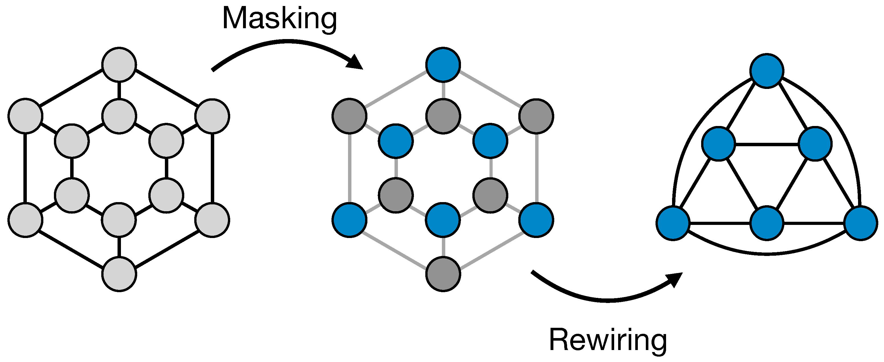
Figure 2. Un-Pooling The un-pool operation consists in embedding the nodes of a pooled graph in their initial position in the bigger original graph structure. All other node’s features are set to 0.

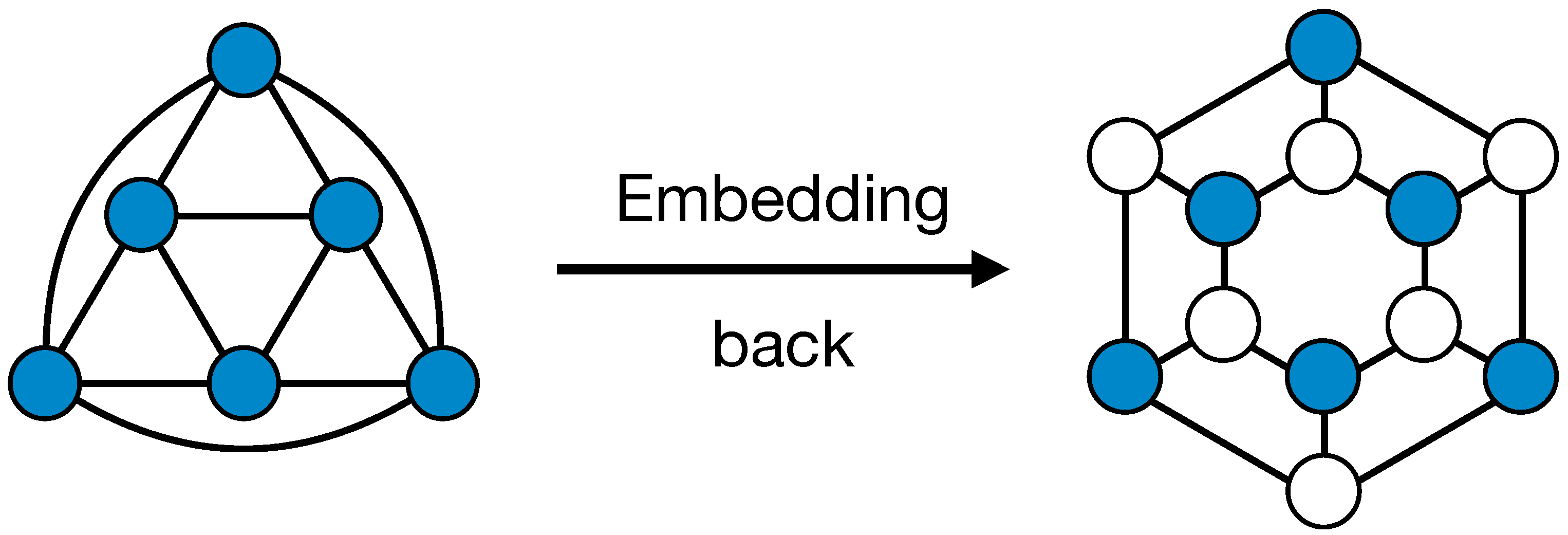
Figure 3. Full scheme Schematic representation of our Re-NN Graph VAE with two encoding blocks and two decoding blocks. Each block is made up by a graph convolution and a pooling (un-pooling) operation. In the lower part of the picture, the reparameterisation trick and the encoding (decoding) linear layers are represented.

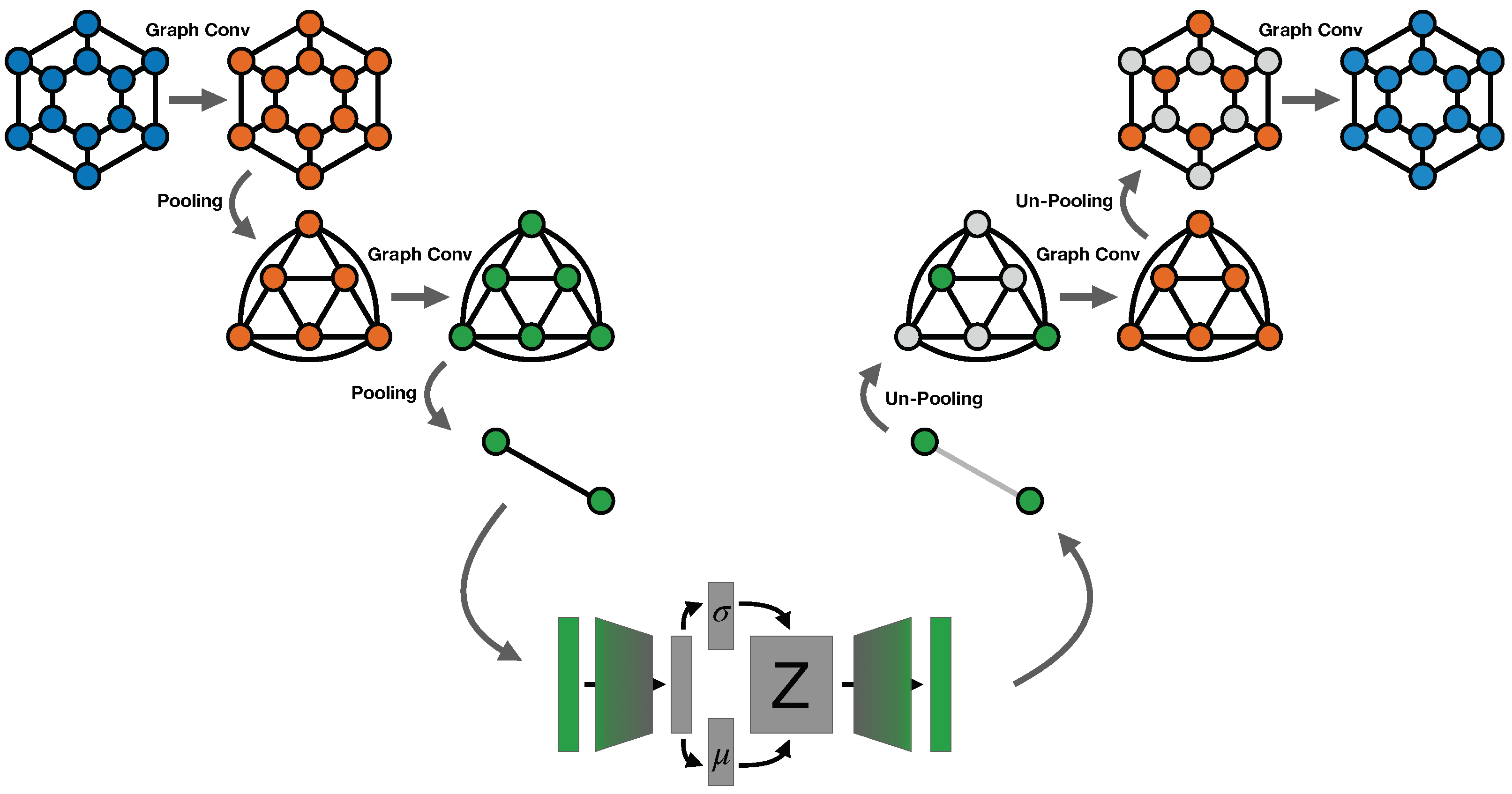
Figure 4. Energy profiles reconstruction. Distribution of energy deposition along z and r axes from the test sets of the Water dataset (a) and the Water + Slice dataset (b). The blue lines correspond to the Monte Carlo simulated data, while the orange lines refer to the reconstructed data from our Network.

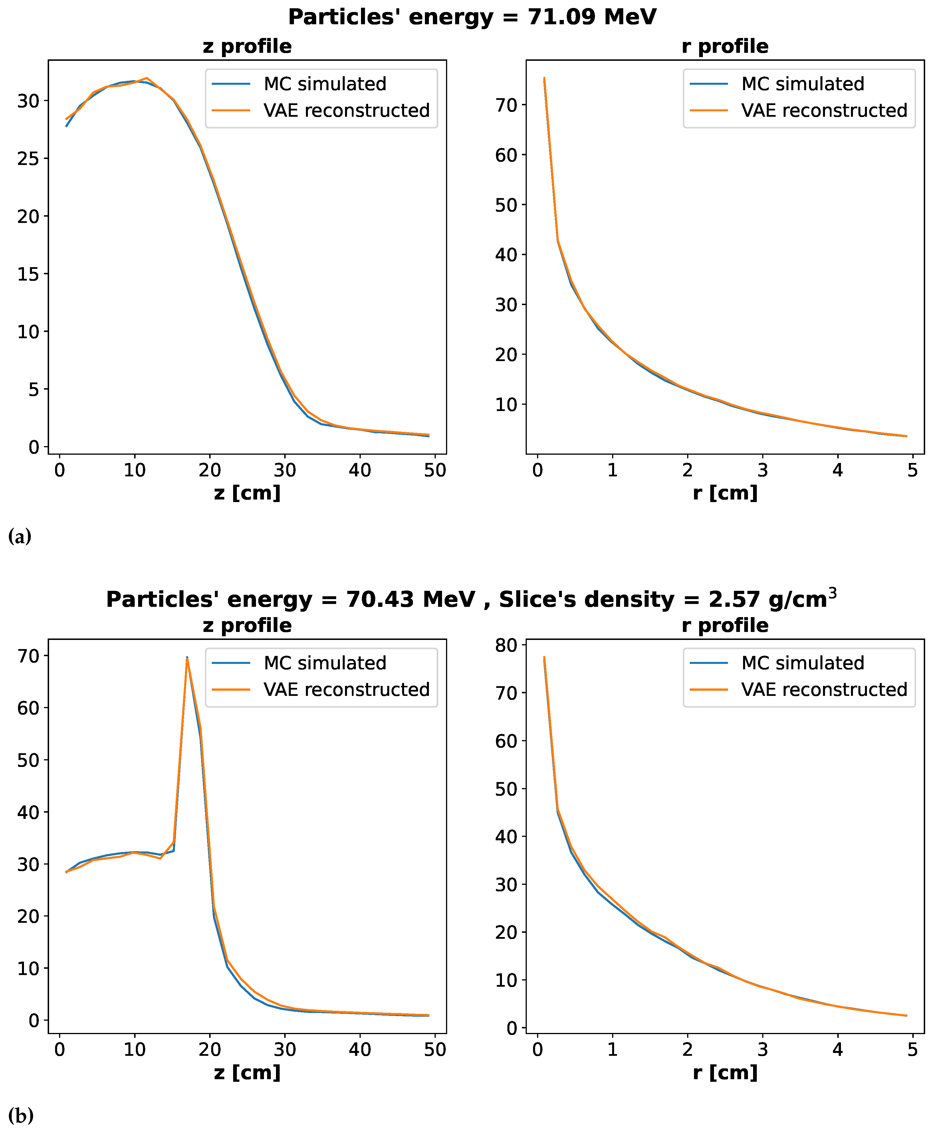
Figure 5. Standard deviations in MC and VAE. Comparison of standard deviation over mean of the energy profile along the Z axis between Monte Carlo simulations and VAE reconstruction in the Water + Slice setting. Values are estimated for 100 MC runs with fixed parameters and 100 VAE execution with the same example as input. Results show how VAE’s largest errors are in regions where energy deposition fluctuation, and so Monte Carlo’s ones, are not negligible.

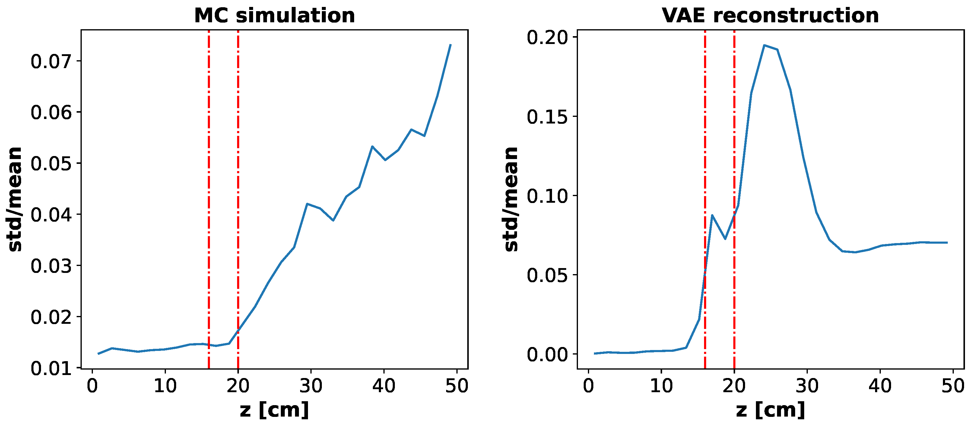
Figure 6. Results on Sprite dataset. (a) Comparison between input sprite images (first row) and reconstructed ones (second row). (b) Images generated fixing all the latent variables’ dimensions but one, which is varied. Generated sprites have fixed attributes but continuously varying hair style.

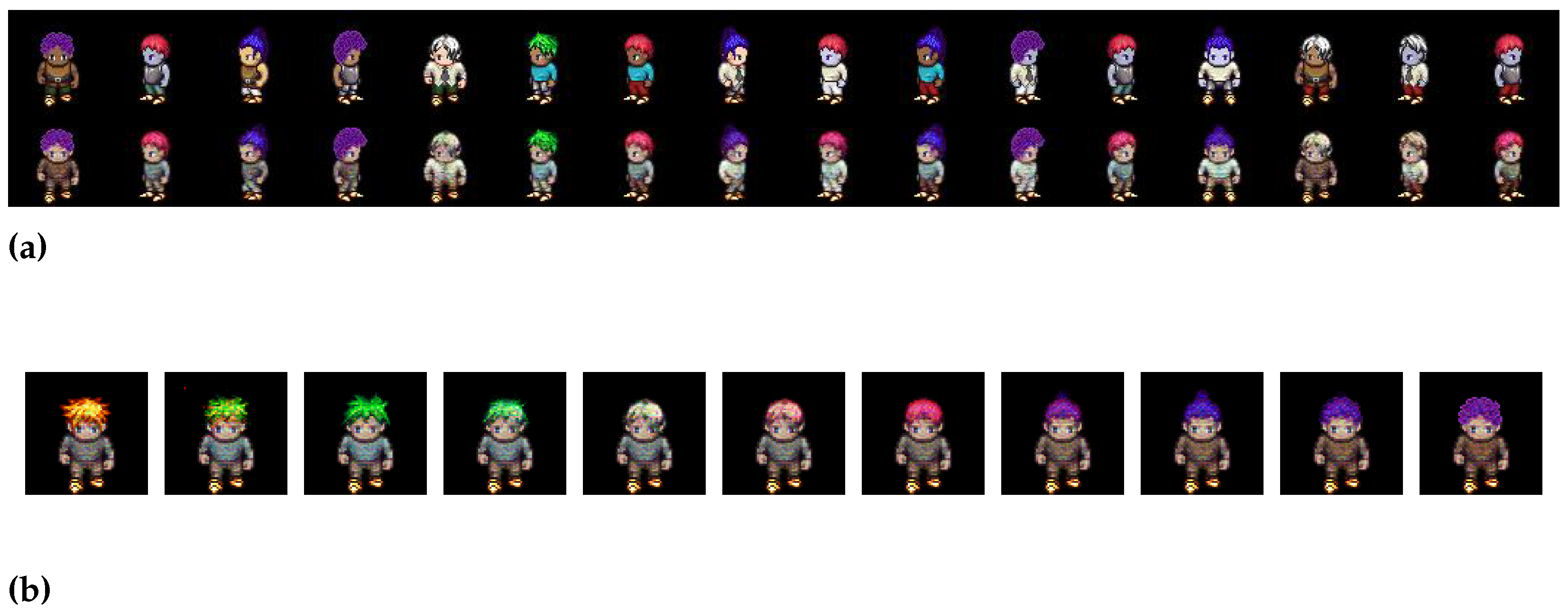
Table 1. Results on energy deposition reconstruction. We report mean relative errors on energy profiles and total energy along with the mean 3%

δ -

index passing rate. Values are computed on test sets

Table 1. Results on energy deposition reconstruction. We report mean relative errors on energy profiles and total energy along with the mean 3%

δ -

index passing rate. Values are computed on test sets

Dataset	Z profile error	R profile error	Total energy error	$δ < 3 %$
Water	5.8 ± 3.4%	2.6 ± 1.6%	2.2 ± 1.6%	99.3 ± 0.1%
Water + Slice	6.9 ± 3.4%	3.0 ± 1.2%	2.2 ± 1.6%	98.6 ± 0.3%

Table 2. Results of ablation study on pooling. We compare results on test set of Water + Slice dataset using different pooling and un-pooling techniques. Mean relative errors on energy profiles and total energy along with the mean 3%

δ -

index passing rate on test sets are reported.

δ -

index passing rate on test sets are reported.

Pooling	Z profile error	R profile error	Total energy error	$δ < 3 %$
ReNN-Pool	6.9 ± 3.4%	3.0 ± 1.2%	2.2 ± 1.6%	98.6 ± 0.3%
Random Pool	172.6 ± 21.7%	52.2 ± 3.7%	2.0 ± 1.5%	92.4 ± 0.4%
Top-k Pool	51.7 ± 3.4%	75.1 ± 9.1%	4.0 ± 2.6%	79.9 ± 1.3%

Disclaimer/Publisher’s Note: The statements, opinions and data contained in all publications are solely those of the individual author(s) and contributor(s) and not of MDPI and/or the editor(s). MDPI and/or the editor(s) disclaim responsibility for any injury to people or property resulting from any ideas, methods, instructions or products referred to in the content.

© 2023 by the authors. Licensee MDPI, Basel, Switzerland. This article is an open access article distributed under the terms and conditions of the Creative Commons Attribution (CC BY) license (http://creativecommons.org/licenses/by/4.0/).

Copyright: This open access article is published under a Creative Commons CC BY 4.0 license, which permit the free download, distribution, and reuse, provided that the author and preprint are cited in any reuse.

Submitted:

30 January 2023

Posted:

02 February 2023

You are already at the latest version

Alerts

Abstract

Keywords:

Subject: Computer Science and Mathematics - Computer Vision and Graphics

1. Introduction

1.1. Related Works

In this section we present relevant works related to Variational Autoencoders, Graph Convolutional layers, pooling and un-pooling operations on graphs.

1.1.1. Variational AutoEncoder

{x}

are the results of a generative process controlled by a variable z that lives in a low dimensional space, called latent space, and their distribution is thus:

p (x) = \int p (x | z) p (z) d z,

where the prior

p (z)

is often considered Gaussian. The model is made up of two networks: the encoder and the decoder. The encoder

q_{ψ} (z | x)

maps the input data to a distribution in the latent space. Thanks to the reparemeterisation trick, a point from such distribution is sampled in a fully differentiable way and processed by the decoder

p_{ψ} (x | z)

to retrieve the original data. The model is trained maximising the evidence lower bound (ELBO) of the data likelihood:

{ψ, ϕ} = a r g m a x_{ψ, ϕ} [E_{x \sim q_{ψ} (\cdot | x)} [l o g p_{ϕ} (x | z) - D_{K L} (q_{ψ} (z | x) | p (z))]]

β > 1

{ψ, ϕ} = a r g m a x_{ψ, ϕ} [E_{x \sim q_{ψ} (\cdot | x)} [l o g p_{ϕ} (x | z) - β D_{K L} (q_{ψ} (z | x) | p (z))]] .

The model with such modification is known as

β -

VAE [16] and is recognised to promote a better disentangling of features’ embedding in the latent space.

1.1.2. Graph generation

In the end, in literature there is no unique and established way to address the problem of graph generation. In this etherogeneous context our main contribution are:

simple, symmetrical and geometry-based pooling and unpooling operations;
a Varational AutoEncoder for regular graph data where both encoding and decoding modules employ graph convolutional layers.

2. Materials and Methods

2.1. Nearest Neighbour Graph VAE

2.1.1. ReNN-Pool and Un-Pool

θ

A^{2}

. We specify that all the adjacency matrices are intended to be binary: element

a_{i j}

is 1 if a link between

i - t h

and

j - t h

node exists and 0 otherwise. So, even after the adjacency augmentation from A to

A^{2}

, the new matrix is binarised. If we call M the vector that contains all the indices of the "surviving" nodes,

X = {x_{i}}_{i = 1}^{N}

and A respectively the nodes’ feature matrix and the adjacency matrix before the pooling, the application of ReNN-Pool gives in output:

\begin{matrix} X^{'} = {x_{i}^{'}}_{i = 1}^{N}, where x_{i}^{'} = \{\begin{matrix} x_{i}, & if i \in M \\ 0, & otherwise \end{matrix} & A^{'} = \{\begin{matrix} A_{i j}^{2}, & if i, j \in M \\ 0, & otherwise \end{matrix} \end{matrix}

The process is illustrated in Figure 1

A^{2}

2.1.2. ReNN Graph VAE architecture

x_{i}^{'} = R e L u (W_{1} x_{i} + W_{2} \frac{1}{| N (i) |} \sum_{j \in N (i)} x_{j}) .

(1)

Eventually, to increase the expressive power of the network, one can also include edge features

e_{i j}

in the computation considering instead:

x_{i}^{'} = R e L u (W_{1} x_{i} + W_{2} \frac{1}{| N (i) |} \sum_{j \in N (i)} e_{i j} x_{j}) .

(2)

In particular, we consider edge features

e_{i j}

to be independent from the nodes’ features and directly learned through a Linear layer.

We chose the output channels of the GraphConv to increase in the three subsequent repetitions, being 16, 32, and 64 channels, as in standard practice.

After the three graph encoding steps, nodes features are put together and flattened. Then, the dimensionality of data is further reduced through a linear layer.

β

-VAE loss function, with binary cross entropy as the reconstruction term.

2.2. Datasets

2.2.1. Energy deposition datasets

The datasets for this task are built simulating an electron beam interacting with a material using Geant4 [30], a toolkit in C++ for Monte Carlo simulations in particle physics.

g / c m^{3}

(for reference, water density is 1

g / c m^{3}

Energy deposition data are collected in a cylindrical scorer, aligned with the electron beam, divided in 28 x 28 x 28 voxels along z,

θ

and r axes. The cylindrical shape is particularly useful in our application because it allows for higher precision near the beamline.

Each example in the dataset is therefore a set of

28^{3}

M e V

. In the Water + Slice Dataset test set, examples have the same range of initial energies and slice’s density values ranging between 2 and 3

g / c m^{3}

. In both cases, the rest of the dataset is used for validation and train with a ratio of

1 / 10

Test sets have been chosen in this way in order to test the network ability to interpolate between samples and generalise to unseen configurations.

For both datasets we imposed a graph structure on data. Each voxels was associated with a node and nodes were linked within each other with a nearest neighbours connectivity.

2.2.2. Sprite dataset

1 / 8

ratio, and 2664 images for test. Each image is

64 x 64

pixels and represents a standing sprite whose attributes are organized in 4 categories (skin color, tops, pants and hairstyle) with 6 variation each, and 3 orientations (left, center and right).

3. Results

3.1. Results on energy deposition datasets

λ = 0.9

. The hyperparameter

β

was set to 1.

δ

index, developed by [32], for its high interpretability. The reconstruction error on each node is thus defined as:

δ = \frac{X_{r e c o} - X_{G T}}{m a x (X_{G T})}

(3)

where

X_{r e c o}

is the node feature predicted by the VAE, while

X_{G T}

is the ground truth node feature in the corresponding example. Then, as reconstruction performance measure we consider the 3% passing rate, which is the percentage of nodes with a

δ

index smaller than 3% . In the Water volume case our Network reaches 99.4% of nodes with 3% passing rate, while in the Water volume + Slice case reaches 98.4% as reported in Table 1.

Total energy: computed summing the features of all nodes.
Z profile: computed integrating, i.e summing, the features of all nodes along the r and $θ$ axes.
R profile: computed integrating, i.e summing, the features of all nodes along the z and $θ$ axes.

3.2. Results on Sprite dataset

λ = 0.95

. In this case the hyperparameter

β

was set to 2.

3.3. Ablation study on pooling

ReNN-Pool: the one proposed in this work,
Random Pool: dropping random nodes in the graph,
Top-k Pool: defined in [23], dropping nodes on the base of features alignment with a learnable vector.

In all cases, for a fair comparison, the number of nodes dropped in each pooling operation is the same. Moreover, after the node dropping, the adjacency matrix is changed from A to

A^{2}

4. Discussion

Author Contributions

Funding

This research received no external funding.

Data Availability Statement

The Sprite dataset is publicly available in https://lpc.opengameart.org/, the Energy deposition datasets and the code used for this study are available on request by contacting the authors.

Conflicts of Interest

Abbreviations

The following abbreviations are used in this manuscript:

CNN	Convolutional Neural Network
GAN	Generative Adversarial Networks
VAE	Variational Auto-Encoder
GNN	Graph Neural Networks
GCN	Graph Convolutional layers
ELBO	Evidence Lower Bound
GAE	Graph Auto-Encoders
VGAE	Variational Graph Auto-Encoders
ReNN-Pool	Recursive Nearest Neighbour Pooling

Appendix A. Full model description

e_{i j}

	Layers	Parameters	N nodes	N edges
Graph Encoder	GraphConv(1, 16, ’mean’)	48	21.952	128.576
	ReNN-Pool	-	10.976	93.960
	GraphConv(16, 32, ’mean’)	1.056	10.976	93.960
	ReNN-Pool	-	1.470	21.952
	GraphConv(32, 64, ’mean’)	4.160	1.470	21.952
	ReNN-Pool	-	236	6.206
	Linear(64 x 236, 64)	966.720	-	-
	Linear(64, 2*)	130	-	-
	Linear(64, 2*)	130	-	-
Graph Decoder	Linear(2*, 64)	192	-	-
	Linear(64, 64 x 236)	981.760	-	-
	ReNN-Unpool	-	1.470	21.952
	GraphConv(64, 32, ’mean’)	4.128	1.470	21.952
	ReNN-Unpool	-	10.976	93.960
	GraphConv(32, 16, ’mean’)	1.040	10.976	93.960
	ReNN-Unpool	-	21.952	128.576
	GraphConv(16, 1, ’mean’)	33	21.952	128.576

Table A2. ReNN Graph VAE for Sprite dataset

	Layers	Parameters	N nodes	N edges
Graph Encoder	GraphConv(3, 16, ’mean’)	112	4.096	16.128
	ReNN-Pool	-	2048	15.874
	Linear(1, 15.874)	31.748	-	-
	GraphConv(16, 32, ’mean’, $e_{i j}$ )	1.056	2048	15.874
	ReNN-Pool	-	528	3.906
	Linear(1, 3.906)	7,812	-	-
	GraphConv(32, 64, ’mean’, $e_{i j}$ )	4.160	528	3.906
	ReNN-Pool	-	136	930
	Linear(64 x 136, 64)	557.120	-	-
	Linear(64, 5)	325	-	-
	Linear(64, 5)	325	-	-
Graph Decoder	Linear(5, 64)	384	-	-
	Linear(64, 64 x 136)	565.760	-	-
	ReNN-Unpool	-	528	3.906
	Linear(1, 3.906)	7,812	-	-
	GraphConv(64, 32, ’mean’, $e_{i j}$ )	4.128	528	3.906
	ReNN-Unpool	-	2.048	15.874
	Linear(1, 15.874)	31.748	-	-
	GraphConv(32, 16, ’mean’, $e_{i j}$ )	1.040	2.048	15.874
	ReNN-Unpool	-	4.096	16.128
	GraphConv(16, 3, ’mean’)	99	4.096	16.128

References

rizhevsky, A.; Sutskever, I.; Hinton, G.E. ImageNet Classification with Deep Convolutional Neural Networks. In Proceedings of the Advances in Neural Information Processing Systems. Curran Associates, Inc., 2012, Vol. 25.
Simonyan, K.; Zisserman, A. Very Deep Convolutional Networks for Large-Scale Image Recognition. Technical report, 2015. arXiv:1409.1556 [cs] type: article. [CrossRef]
He, K.; Zhang, X.; Ren, S.; Sun, J. Deep Residual Learning for Image Recognition. Technical report, 2015. arXiv:1512.03385 [cs] type: article. [CrossRef]
Bond-Taylor, S.; Leach, A.; Long, Y.; Willcocks, C.G. Deep Generative Modelling: A Comparative Review of VAEs, GANs, Normalizing Flows, Energy-Based and Autoregressive Models. IEEE Transactions on Pattern Analysis and Machine Intelligence 2022, 44, 7327–7347. arXiv:2103.04922 [cs, stat]. [CrossRef]
Goodfellow, I.J.; Pouget-Abadie, J.; Mirza, M.; Xu, B.; Warde-Farley, D.; Ozair, S.; Courville, A.; Bengio, Y. Generative Adversarial Networks. Technical report, 2014. arXiv:1406.2661 [cs, stat] type: article. [CrossRef]
Kingma, D.P.; Welling, M. Auto-Encoding Variational Bayes. Technical report, 2014. arXiv:1312.6114 [cs, stat] type: article. [CrossRef]
LeCun, Y.; Chopra, S.; Hadsell, R.; Ranzato, A.; Huang, F. A Tutorial on Energy-Based Learning. 2006.
Rezende, D.; Mohamed, S. Variational Inference with Normalizing Flows. In Proceedings of the Proceedings of the 32nd International Conference on Machine Learning; Bach, F.; Blei, D., Eds.; PMLR: Lille, France, 2015; Vol. 37, Proceedings of Machine Learning Research, pp. 1530–1538.
Sohl-Dickstein, J.; Weiss, E.; Maheswaranathan, N.; Ganguli, S. Deep Unsupervised Learning using Nonequilibrium Thermodynamics. In Proceedings of the Proceedings of the 32nd International Conference on Machine Learning; Bach, F.; Blei, D., Eds.; PMLR: Lille, France, 2015; Vol. 37, Proceedings of Machine Learning Research, pp. 2256–2265.
Morris, C.; Ritzert, M.; Fey, M.; Hamilton, W.L.; Lenssen, J.E.; Rattan, G.; Grohe, M. Weisfeiler and Leman Go Neural: Higher-order Graph Neural Networks. Technical report, 2021. arXiv:1810.02244 [cs, stat] type: article. [CrossRef]
Kipf, T.N.; Welling, M. Semi-Supervised Classification with Graph Convolutional Networks. Technical report, 2017. arXiv:1609.02907 [cs, stat] type: article. [CrossRef]
Defferrard, M.; Bresson, X.; Vandergheynst, P. Convolutional Neural Networks on Graphs with Fast Localized Spectral Filtering. Technical report, 2017. arXiv:1606.09375 [cs, stat] type: article. [CrossRef]
Veličković, P.; Cucurull, G.; Casanova, A.; Romero, A.; Liò, P.; Bengio, Y. Graph Attention Networks. Technical report, 2018. arXiv:1710.10903 [cs, stat] type: article. [CrossRef]
Zhu, Y.; Du, Y.; Wang, Y.; Xu, Y.; Zhang, J.; Liu, Q.; Wu, S. A Survey on Deep Graph Generation: Methods and Applications. Technical report, 2022. arXiv:2203.06714 [cs, q-bio] type: article. [CrossRef]
Wu, Z.; Pan, S.; Chen, F.; Long, G.; Zhang, C.; Yu, P.S. A Comprehensive Survey on Graph Neural Networks. IEEE Transactions on Neural Networks and Learning Systems 2021, 32, 4–24. arXiv:1901.00596 [cs, stat]. [CrossRef]
Higgins, I.; Matthey, L.; Pal, A.; Burgess, C.; Glorot, X.; Botvinick, M.; Mohamed, S.; Lerchner, A. beta-VAE: Learning Basic Visual Concepts with a Constrained Variational Framework. 2022.
Kipf, T.N.; Welling, M. Variational Graph Auto-Encoders. Technical report, 2016. arXiv:1611.07308 [cs, stat] type: article. [CrossRef]
Dhillon, I.S.; Guan, Y.; Kulis, B. Weighted Graph Cuts without Eigenvectors A Multilevel Approach. IEEE Transactions on Pattern Analysis and Machine Intelligence 2007, 29, 1944–1957. [CrossRef]
Zhang, M.; Cui, Z.; Neumann, M.; Chen, Y. An End-to-End Deep Learning Architecture for Graph Classification. Proceedings of the AAAI Conference on Artificial Intelligence 2018, 32. [Google Scholar] [CrossRef]
Bianchi, F.M.; Grattarola, D.; Livi, L.; Alippi, C. Hierarchical Representation Learning in Graph Neural Networks with Node Decimation Pooling. IEEE Transactions on Neural Networks and Learning Systems 2022, 33, 2195–2207, arXiv:1910.11436 [cs, math, stat]. [Google Scholar] [CrossRef] [PubMed]
Bravo-Hermsdorff, G.; Gunderson, L.M. A Unifying Framework for Spectrum-Preserving Graph Sparsification and Coarsening. Technical report, 2020. arXiv:1902.09702 [cs] type: article. [CrossRef]
Ying, R.; You, J.; Morris, C.; Ren, X.; Hamilton, W.L.; Leskovec, J. Hierarchical Graph Representation Learning with Differentiable Pooling. Technical report, 2019. arXiv:1806.08804 [cs, stat] type: article. [CrossRef]
Gao, H.; Ji, S. Graph U-Nets. Technical report, 2019. arXiv:1905.05178 [cs, stat] type: article. [CrossRef]
Guo, Y.; Zou, D.; Lerman, G. An Unpooling Layer for Graph Generation. Technical report, 2022. arXiv:2206.01874 [cs, stat] type: article. [CrossRef]
Liu, Q.; Allamanis, M.; Brockschmidt, M.; Gaunt, A.L. Constrained Graph Variational Autoencoders for Molecule Design. Technical report, 2019. arXiv:1805.09076 [cs, stat] type: article. [CrossRef]
Bresson, X.; Laurent, T. A Two-Step Graph Convolutional Decoder for Molecule Generation. Technical report, 2019. arXiv:1906.03412 [cs, stat] type: article. [CrossRef]
Guo, X.; Zhao, L.; Qin, Z.; Wu, L.; Shehu, A.; Ye, Y. Interpretable Deep Graph Generation with Node-Edge Co-Disentanglement. In Proceedings of the Proceedings of the 26th ACM SIGKDD International Conference on Knowledge Discovery & Data Mining, 2020, pp. 1697–1707. arXiv:2006.05385 [cs, stat]. [CrossRef]
Assouel, R.; Ahmed, M.; Segler, M.H.; Saffari, A.; Bengio, Y. DEFactor: Differentiable Edge Factorization-based Probabilistic Graph Generation. Technical report, 2018. arXiv:1811.09766 [cs] type: article. [CrossRef]
Du, Y.; Guo, X.; Cao, H.; Ye, Y.; Zhao, L. Disentangled Spatiotemporal Graph Generative Models. Proceedings of the AAAI Conference on Artificial Intelligence 2022, 36, 6541–6549. [Google Scholar] [CrossRef]
Agostinelli, S.; Allison, J.; Amako, K.; Apostolakis, J.; Araujo, H.; Arce, P.; Asai, M.; Axen, D.; Banerjee, S.; Barrand, G.; et al. Geant4—a simulation toolkit. Nuclear Instruments and Methods in Physics Research Section A: Accelerators, Spectrometers, Detectors and Associated Equipment 2003, 506, 250–303. [Google Scholar] [CrossRef]
Li, Y.; Mandt, S. Disentangled Sequential Autoencoder. Technical report, 2018. arXiv:1803.02991 [cs] type: article. [CrossRef]
Mentzel, F.; Kröninger, K.; Lerch, M.; Nackenhorst, O.; Paino, J.; Rosenfeld, A.; Saraswati, A.; Tsoi, A.C.; Weingarten, J.; Hagenbuchner, M.; et al. Fast and accurate dose predictions for novel radiotherapy treatments in heterogeneous phantoms using conditional 3D-UNet generative adversarial networks. Medical Physics 2022, 49, 3389–3404. [Google Scholar] [CrossRef] [PubMed]

1	https://lpc.opengameart.org/
2	https://github.com/sanderfrenken/Universal-LPC-Spritesheet-Character-Generator
3	https://github.com/YingzhenLi/Sprites

Table 1. Results on energy deposition reconstruction. We report mean relative errors on energy profiles and total energy along with the mean 3%

δ -

index passing rate. Values are computed on test sets

Table 1. Results on energy deposition reconstruction. We report mean relative errors on energy profiles and total energy along with the mean 3%

δ -

index passing rate. Values are computed on test sets

Dataset	Z profile error	R profile error	Total energy error	$δ < 3 %$
Water	5.8 ± 3.4%	2.6 ± 1.6%	2.2 ± 1.6%	99.3 ± 0.1%
Water + Slice	6.9 ± 3.4%	3.0 ± 1.2%	2.2 ± 1.6%	98.6 ± 0.3%

δ -

index passing rate on test sets are reported.

δ -

index passing rate on test sets are reported.

Pooling	Z profile error	R profile error	Total energy error	$δ < 3 %$
ReNN-Pool	6.9 ± 3.4%	3.0 ± 1.2%	2.2 ± 1.6%	98.6 ± 0.3%
Random Pool	172.6 ± 21.7%	52.2 ± 3.7%	2.0 ± 1.5%	92.4 ± 0.4%
Top-k Pool	51.7 ± 3.4%	75.1 ± 9.1%	4.0 ± 2.6%	79.9 ± 1.3%

MDPI Initiatives

Important Links

Choose an area of interest and we will send you notifications of new preprints at your preferred frequency.

Disclaimer

Nearest Neighbours Graph Variational AutoEncoder

Abstract

1. Introduction

1.1. Related Works

1.1.1. Variational AutoEncoder

1.1.2. Graph generation

2. Materials and Methods

2.1. Nearest Neighbour Graph VAE

2.1.1. ReNN-Pool and Un-Pool

2.1.2. ReNN Graph VAE architecture

2.2. Datasets

2.2.1. Energy deposition datasets

2.2.2. Sprite dataset

3. Results

3.1. Results on energy deposition datasets

3.2. Results on Sprite dataset

3.3. Ablation study on pooling

4. Discussion

Author Contributions

Funding

Data Availability Statement

Conflicts of Interest

Abbreviations

Appendix A. Full model description

References

Abstract

1. Introduction

1.1. Related Works

1.1.1. Variational AutoEncoder

1.1.2. Graph generation

2. Materials and Methods

2.1. Nearest Neighbour Graph VAE

2.1.1. ReNN-Pool and Un-Pool

2.1.2. ReNN Graph VAE architecture

2.2. Datasets

2.2.1. Energy deposition datasets

2.2.2. Sprite dataset

3. Results

3.1. Results on energy deposition datasets

3.2. Results on Sprite dataset

3.3. Ablation study on pooling

4. Discussion

Author Contributions

Funding

Data Availability Statement

Conflicts of Interest

Abbreviations

Appendix A. Full model description

References

MDPI Initiatives

Important Links

Subscribe