Human Movements Are Shaped by Utilizing Sensory Information: A Stochastic Optimum Model

Preprint

Article

Human Movements Are Shaped by Utilizing Sensory Information: A Stochastic Optimum Model

Altmetrics

Downloads

171

Views

Comments

Mehran Emadi Andani^*

This version is not peer-reviewed

This preprints belongs to the Topic

Bio-Inspired Systems and Signal Processing

Submitted:

02 February 2023

Posted:

03 February 2023

You are already at the latest version

Alerts

Abstract

Human motor planning combines such interesting aspects as modular organization in motor primitives and characteristics of stochastic optimality. Motor primitives aided in the description of motor skill learning. In this study, for the first time, an interpretation is proposed to explain how motor primitives are shaped in a stochastic optimality process.To this end, sensory information is assumed to be random variables at each moment. Theoretically, the results confirmed that the variability of a movement increased with passing time. As a result, motor planning should be performed in shorter durations to achieve an accurate movement. It means that a task should be divided into several subtasks at various stages of time. Moreover, theoretically, the results confirmed that motor planning is statistically optimal if the movement is planned in minimum jerk space, which is in accordance with what is reported in the literature. Comparing the proposed mathematical model with the results of experimental data in two different types of motor action (i.e., arm reaching movement and sit-to-stand transfer from a chair) confirmed that the proposed model can be considered a framework to investigate the effect of bottom-up information on human motor planning level. Further experiments need to investigate it more deeply.

Keywords:

Subject: Engineering - Bioengineering

Introduction

There is variability in human movement planning due to the abundance of degree of freedom. It means that there are infinite ways to plan a movement, but humans perform the movements more or less similarly, although there is variability. Researchers demonstrated in various studies that using the minimum jerk policy to plan a movement is one possible policy (Emadi Andani et al., 2012; Friedman et al., 2009).

The movements of limbs and bodies to carry out motor tasks or interact with the environment, which appear to be commonplace behaviors, are incredibly complex. To go to a destination, we must first perceive its location in relation to an outside coordinate system. The next step is to plan a limb trajectory, which is then carried out by giving the muscles the proper sequence of brain signals. These in turn provide the proper forces and torques to the joints, causing the arm to move in the correct direction. Here, we examine some of the early research on human movement control as well as some more contemporary works on the subject, with a particular emphasis on behavioral and modeling studies addressing task space and joint-space movement planning. We provide research on trajectory planning and inverse kinematics issues during point-to-point reaching motions, as well as two- and three-dimensional drawing actions, at the task level. In particular, differential geometrical techniques that address the relationship between path geometry and movement velocity are covered in our discussion of models dealing with the two-thirds power law. We also talk about isochrony and minimum-jerk models for curved and point-to-point motions, among other optimization ideas.

Methods and Materials

Let us assume g(t) is a movement performed by a healthy individual. The movement can be described by joint angles or by end-point positions in cartesian coordinates. Let’s suppose that sensory information provides the kinematic information (position, velocity, and acceleration) of the biomechanical system at the initial moment. Since there is a delay in perceiving sensory information, it would be more accurate if the biomechanical system remained stable in a static position for a while before starting the movement.

Assuming g(t) is a random variable, according to Appendix A, the position (

g (t)

), velocity (

\dot{g} (t)

) and acceleration (

\ddot{g} (t)

) have a Gaussian distribution function as follows:

\ddot{g} (t) : T_{2} (m_{\ddot{g}} (t), σ_{\ddot{g}}^{2} (t))

(1)

\dot{g} (t) : T_{1} (m_{\dot{g}} (t), σ_{\dot{g}}^{2} (t))

(2)

g (t) : T_{0} (m_{g} (t), σ_{g}^{2} (t))

(3)

where,

m_{\ddot{g}} (t)

m_{\dot{g}} (t)

and

m_{g} (t)

are the mean values, and

σ_{\ddot{g}}^{2} (t)

σ_{\dot{g}}^{2} (t))

and

σ_{g}^{2} (t)

are the variances of

\ddot{g} (t)

\dot{g} (t)

and

g (t)

, respectively.

According to (A29) in Appendix A, the following relations can be written.

m_{\dot{g}} (t) = m_{\dot{g}} (0) + \int_{0}^{t} m_{\ddot{g}} (t') d t'

(4)

m_{g} (t) = m_{g} (0) + \int_{0}^{t} m_{\dot{g}} (t') d t'

(5)

σ_{\dot{g}}^{2} (t) = σ_{\dot{g}}^{2} (0) + \int_{t^{'} = 0}^{t} \int_{t^{″} = 0}^{t'} C o v (\ddot{g} (t^{'}), \ddot{g} (t^{″})) d t^{″} d t^{'}

(6)

σ_{g}^{2} (t) = σ_{g}^{2} (0) + \int_{t^{'} = 0}^{t} \int_{t^{''} = 0}^{t'} C o v (\dot{g} (t^{'}), \dot{g} (t^{″})) d t^{″} d t^{'}

(7)

However, there is evidence to show that the central nervous system (CNS) predicts the performed movement (Flanagan & Wing, 1997; Vaziri, Diedrichsen, & Shadmehr, 2006). Assume that y(t) is a prediction or estimate of the performed movement.

Due to the lack of information about the statistical properties of the distribution, an unweighted least-squares estimator is well suited, as described in (8). Based on this criterion, the best estimation is the argument of the following objective function, described as (9).

J = \int_{0}^{t_{f}} {(y (t') - g (t'))}^{2} d t

(8)

y_{o p t i m u m} = A r g (M i n (E [J]))

(9)

As proved in Appendix B, the solution to this optimization is:

y_{o p t i m u m} = E [g (t)]

(10)

y_{o p t i m u m} = m_{g} (t)

(11)

Let us assume another objective function as follows:

J_{1} = \int_{0}^{t_{f}} {(\dot{y} (t') - \dot{g} (t'))}^{2} d t

(12)

The solution to (12) is:

{\dot{y}}_{o p t i m u m} (t) = m_{\dot{g}} (t)

(13)

It means that:

y_{o p t i m u m} (t) = \int_{0}^{t} m_{\dot{g}} (t') d t + k_{1}

(14)

Using (5), one can conclude that (14) and (11) are equivalent if

k_{1} = m_{g} (0)

. It means that the objective functions (8) and (12) are equivalent if

m_{g} (0)

is known. Similarly, if we know the initial position, velocity, …, and the (k-1)^th derivative of the g(t), we can show that the arguments for minimizing J and J_k (defined in (15)) are equivalent.

J_{k} = \int_{0}^{t_{f}} {(\frac{d^{k} y (t)}{{d t}^{k}} - \frac{d^{k} g (t)}{{d t}^{k}})}^{2} d t

(15)

On the other hand, in the human motor system, sensory information provides the information corresponding to position, velocity, and acceleration, i.e.,

m_{g} (0)

m_{\dot{g}} (0)

and

m_{\ddot{g}} (0)

. In this case, it can be said that J and J₃ are equivalent, and minimizing them results in the same solution (

y_{o p t i m u m}

). Based on the computational point of view, searching in

\overset{⃛}{y} (t)

space is easier than searching in

y (t)

space because of the constraints of initial conditions. Therefore, it is reasonable to consider J₃ as having the main objective function for searching in

\overset{⃛}{y} (t)

space.

To calculate movement variability, we suppose that the covariance matrix has a simple exponential form described as (16) (Appendix C).

C o v (\overset{⃛}{g} (t^{'}), \overset{⃛}{g} (t^{″})) = σ_{0}^{2} e^{- \frac{|t^{''} - t^{'}|}{τ_{3}}}

(16)

where,

τ_{3}

is a time constant to scale the time span. If t' and t" are close, or equivalently

τ_{3}

is big, the covariance value is higher, meaning that

\overset{⃛}{g} (t^{'})

and

\overset{⃛}{g} (t^{''})

are more correlated. On the contrary, if t' and t" are far from each other, or equivalently

τ_{3}

is small, the covariance value is less, meaning that

\overset{⃛}{g} (t^{'})

and

\overset{⃛}{g} (t^{''})

are less correlated.

Inspired by (6), we can write (17). Using (16) and (17), we can write (18).

σ_{\ddot{g}}^{2} (t) = σ_{\ddot{g}}^{2} (0) + 2 \int_{t^{'} = 0}^{t} \int_{t^{''} = 0}^{t'} C o v (\overset{⃛}{g} (t'), \overset{⃛}{g} (t^{″})) d t^{″} d t^{'}

(17)

σ_{\ddot{g}}^{2} (t) = {σ_{\ddot{g}}^{2} (0) + 2 σ}_{0}^{2} τ_{3} (t - τ_{3} (1 - e^{- \frac{t}{τ_{3}}}))

(18)

In order to simplify the formula, for

\frac{t}{τ_{3}} ≫ 1

, we can write:

σ_{\ddot{g}}^{2} (t) ≅ {σ_{\ddot{g}}^{2} (0) + 2 σ}_{0}^{2} τ_{3} t

(19)

With a same covariance function, we have:

σ_{\dot{g}}^{2} (t) ≅ σ_{\dot{g}}^{2} (0) + 2 \int_{t^{'} = 0}^{t} \int_{t^{''} = 0}^{t'} {(σ_{\ddot{g}}^{2} (0) + 2 σ}_{0}^{2} τ_{3} t'' {) e}^{(t^{''} - t^{'}) / τ_{2}} d t^{″} d t'

(20)

σ_{\dot{g}}^{2} (t) ≅ σ_{\dot{g}}^{2} (0) + {2 σ}_{\ddot{g}}^{2} (0) τ_{2} t + \int_{t^{'} = 0}^{t} {(4 σ}_{0}^{2} τ_{2} τ_{3} t'') {(1 - e}^{- \frac{t^{''}}{τ_{2}}}) d t'

(21)

σ_{\dot{g}}^{2} (t) ≅ σ_{\dot{g}}^{2} (0) + 2 σ_{\ddot{g}}^{2} (0) τ_{2} t + {4 σ}_{0}^{2} τ_{2} τ_{3} (\frac{1}{2} t^{2} + τ_{2} t e^{- \frac{t}{τ_{2}}} + {τ_{2}}^{2} {(1 - e}^{- \frac{t}{τ_{2}}}))

(22)

Similarly, for

\frac{t}{τ_{2}} ≫ 1

, we can write:

σ_{\dot{g}}^{2} (t) ≅ σ_{\dot{g}}^{2} (0) + 2 σ_{\ddot{g}}^{2} (0) τ_{2} t + 2 σ_{0}^{2} τ_{2} τ_{3} t^{2}

(23)

Again, with a same covariance function for

g

, we have:

σ_{g}^{2} (t) ≅ σ_{g}^{2} (0) + 2 \int_{t^{'} = 0}^{t} \int_{t^{''} = 0}^{t'} {(σ}_{\dot{g}}^{2} (0) + {2 σ}_{\ddot{g}}^{2} (0) τ_{2} t^{″} + 2 σ_{0}^{2} τ_{2} τ_{3} {t^{''}}^{2}) e^{- (t^{''} - t^{'}) / τ_{1}} d t^{″} d t'

(24)

Finally, for

\frac{t}{τ_{1}} ≫ 1

, we can write:

σ_{g}^{2} (t) ≅ σ_{g}^{2} (0) + {2 σ}_{\dot{g}}^{2} (0) τ_{1} t + 2 σ_{\ddot{g}}^{2} (0) τ_{1} τ_{2} t^{2} + \frac{4}{3} σ_{0}^{2} τ_{1} τ_{2} τ_{3} t^{3}

(25)

Chosen tasks. To evaluate the proposed model from a behavioral point of view, we analyzed two types of daily movements studied frequently in the field of motor control: arm reaching movement (Bhushan & Shadmehr, 1999; Darainy, Malfait, Gribble, Towhidkhah, & Ostry, 2004; Haruno,Wolpert, & Kawato, 2003; Haruno, Wolpert, & Kawato, 2001) and sit-to-stand (STS) transfer from a chair (Bahrami, Riener, Jabedar-Maralani, & Schmidt, 2000; Craig, 2005; Emadi Andani, Bahrami, & Maralani, 2007, 2009; Janssen, Bussmann, & Stam, 2002).

Arm reaching movement. Participants were asked to reach a visual target in front of them located 20 cm away from the hand (Darainy et al., 2004). The position of the hand was recorded, and the shoulder and elbow joint angles of one arm in the horizontal plane were calculated from the recorded data (Darainy et al., 2004). Each participant performed the task for 100 trials. Data were aligned based on starting the task.

STS. Participants were asked to perform a sit-to-stand transfer from a chair task. The trajectories of joint angles of one side of the body in the sagittal plane were recorded (Bahrami, Moraes, & Patla, 2003). Each participant performed the task for 20 trials. Data were aligned based on the seat-off moment.

Results

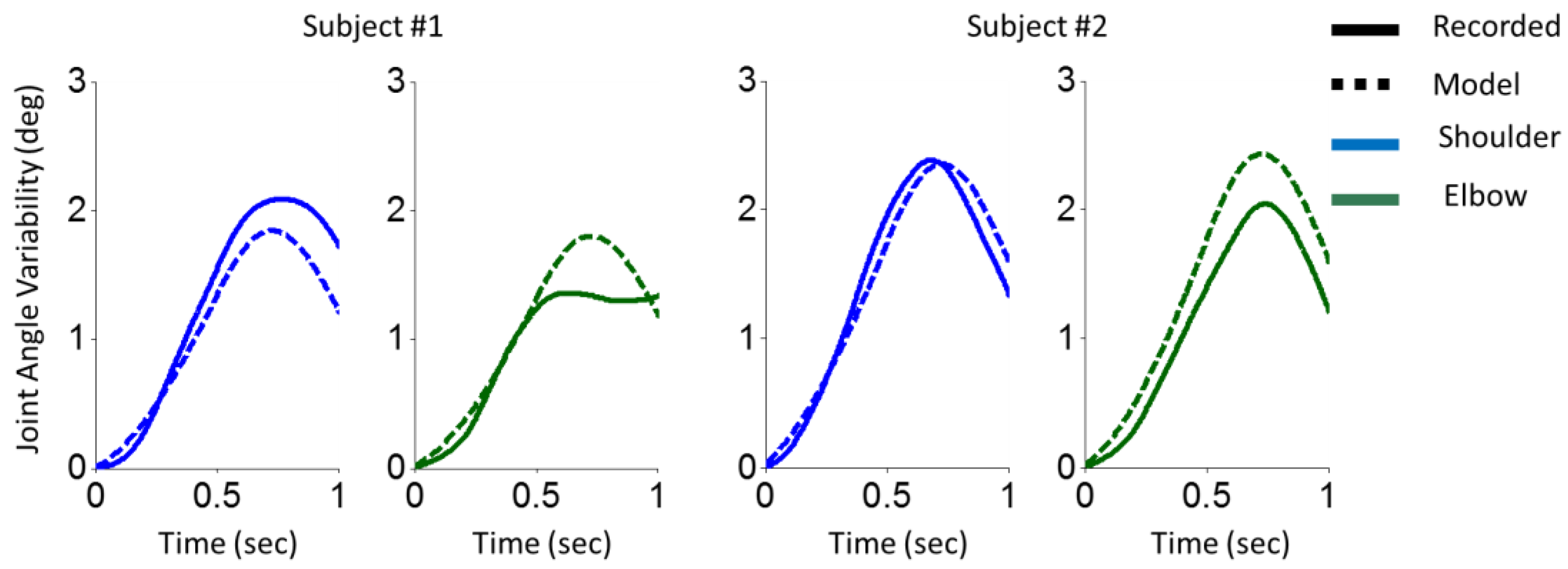
The results of arm reaching movements for two representative subjects are illustrated in Figure 1. The parameters of the model simply were set at

τ_{1} {= τ}_{2} = τ_{3} = 70 m s

. The results of the proposed model predict increasing movement variability a time passes.

In order to decrease the prediction error of the model, the correlation window should be decreased. To this end, τ₁, τ₂ and τ₃ decreased gradually after

t_{0}

= 500 ms of the movement onset described in (26);

τ = τ_{1} {= τ}_{2} = τ_{3}

τ = \{\begin{matrix} τ_{0} & t \leq t_{0} \\ τ_{0} e^{- a {(t - t_{0})}^{2}} & t > t_{0} \end{matrix}

(26)

Applying this modification, the results of arm reaching movements for two representative participants are illustrated in Figure 2. Statistical analysis of Pearson correlation on arm reaching movement data revealed that the model and experimental results were significantly correlated (shoulder: r = 0.99, p < 0.001; r = 0.97, elbow: p < 0.001).

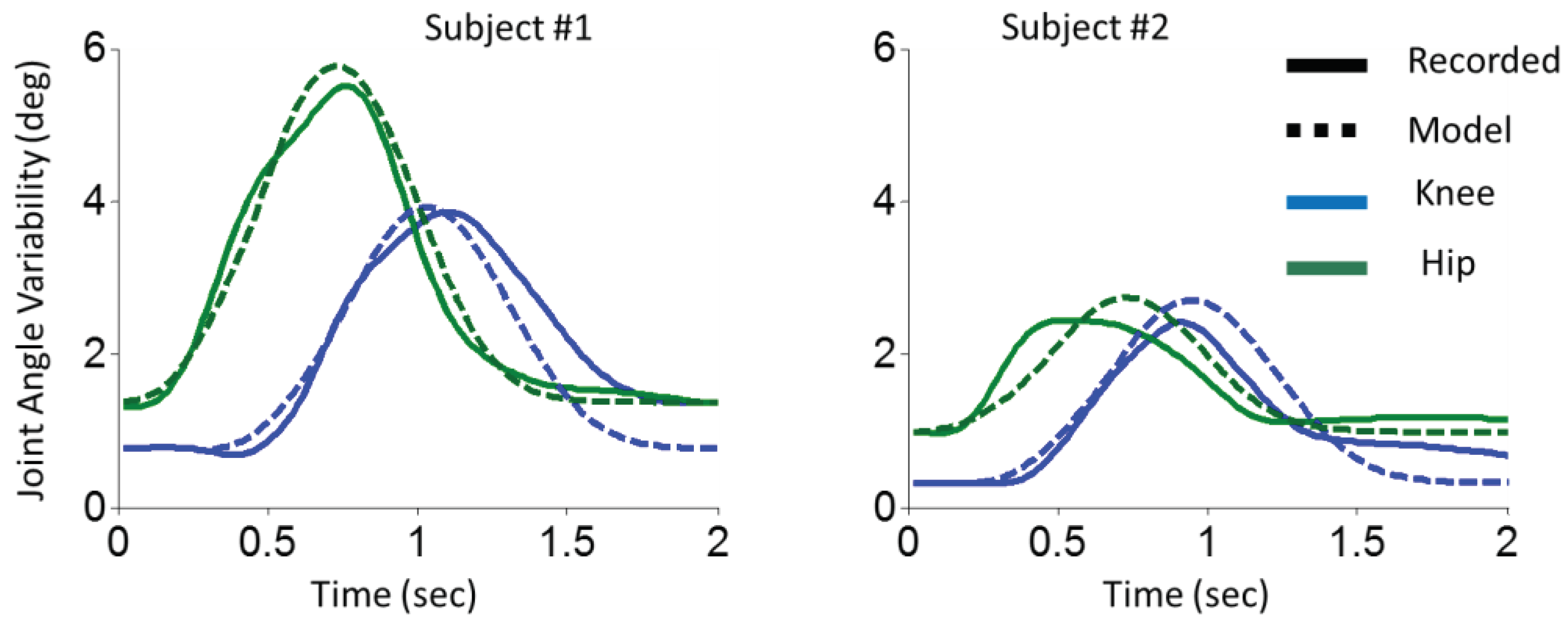
The results of STS transfer are illustrated for two representative participants in Figure 3. The same modification was applied to the model for the STS experiment. Statistical analysis of Pearson correlation on STS data revealed that the model and experimental results were significantly correlated (knee: r = 0.82, p < 0.001; r = 0.80, hip: p < 0.001).

Discussion and conclusion

Faster movement, less movement variability. Theoretical formulation, specifically (24), showed that the variability of a movement increases with passing time. It means that the discrepancy between different performed trials and, also, between performed trials and the planned movement can be significantly different at the end of the movement. The longer the movement duration, the greater the difference at the end of the trials. In another word, in a given path, the variation of the movement is higher for the movements performed slower, which take more time to complete.

Motor decomposition to decrease movement variability. In order to control the variability of the movement, the covariance function can be narrowed by adjusting

τ_{1}, τ_{2}

and

τ_{3}

. If they are zero (i.e.,

g (t)

is i.i.d) the variance of

g (t)

will be at the lowest level and constant (i.e.,

σ_{g}^{2} (0)

). On the other hand, planning a movement with high correlation facilitates more accurate prediction of the movement and it helps compensate for the delay in sensory information. However, the proposed model showed that planning a movement with high correlation increases the movement’s variability over time. Therefore, there is a trade-off between movement variability and accuracy of prediction. For very short movements, a possible way is to start the movement with high correlation (to use the benefit of feedback from sensory information) and then gradually switch to low correlation (performing a feedforward control). Another possible solution for longer tasks is to decompose the movement into several sub-tasks. In this case, in each sub-task, the movement prediction is done accurately, and the time duration is reset for each sub-task in order to bound the variability in a certain range. Based on this point of view and by looking at the results in Figure 1, one can conclude that ARM has two sub-tasks; you can see a decrease in the variability after 0.6 sec (for subject #1) and 0.7 sec (for subject #2). In order to plan a movement, the CNS may consider this possible solution, i.e., motor decomposition.

Minimum-jerk model. As mentioned before,

g (t)

is the performed movement, and

y (t)

is the estimated movement by the CNS. Let us assume that J₃ is defined as:

J_{3} = \int_{0}^{t_{f}} {(\overset{⃛}{y} (t) - \overset{⃛}{g} (t))}^{2} d t

(27)

Then, we have:

J_{3} = \underset{A}{\underset{⏟}{\int_{0}^{t_{f}} {(\overset{⃛}{y} (t))}^{2} d t}} + \underset{B}{\underset{⏟}{\int_{0}^{t_{f}} {(\overset{⃛}{g} (t))}^{2} d t}} - 2 \underset{C}{\underset{⏟}{\int_{0}^{t_{f}} \overset{⃛}{y} (t) \overset{⃛}{g} (t) d t}}

(28)

As the term “B” includes the performed movement and is constant, minimizing J₃ can be achieved by maximizing C and minimizing A. Since

g (t)

is not known, one suboptimal solution for minimizing J₃ is to find the projection of

y

g

(in order to maximize C) in the space that A remains minimum, i.e., the minimum jerk space. In other words, y is a projection of

g

onto the minimum jerk space. This solution can be optimal if

g

is also planned/performed in a minimum jerk space. It means that the desired movement should be planned with minimum jerk space to increase the accuracy of the estimation. Different researchers have reported that one possible model to describe human motor planning is the minimum jerk model (Emadi Andani & Bahrami, 2012; Flash & Hogan, 1985; Friedman & Flash, 2009). Interestingly, six general movement elements (a type of motor primitive) in minimum jerk space have already been introduced by Emadi (Andani and Bahrami 2012). It means that any minimum jerk movement can be generated easily by the linear combination of the six general movement elements.

Motor decomposition and the minimum jerk model. Considering motor decomposition and the minimum jerk model, it is reasonable to conclude that a possible policy to plan a movement by the CNS can be described using motor decomposition and planning in minimum jerk space, as reported in (Emadi Andani & Bahrami, 2012).

Stochastic optimal solution. Stochastic optimal solutions can be obtained by evolutionary methods during human life. Evolution has an important role in using sensory information to plan a movement.

As future work, it could be interesting to study the movement planned with less sensory information. For instance, if the sensors corresponding to acceleration (I mean, GTO sensors) do not work accurately because of a disease, the movement planning space must be changed to a minimum acceleration space, according to our proposed model. In this case, these patients with this disease plan their desired movements in the minimum acceleration space. It can also be studied more deeply in the movements performed by the animals without acceleration and/or velocity sensors.

Although we cannot guarantee that any given movement satisfies the minimum angle jerk condition, we might be able to decompose each task into its subtasks, where each subtask satisfies this constraint. In this case, each subtask, or each phase of the movement, will be defined by a linear combination of the proposed MEs.

Acknowledgments

I would like to thank Dr. Fariba Bahrami and Dr. Renato Moraes for sharing the data of sit-to-stand transfer from a chair. These data were recorded in the Gait and Posture Laboratory (GAPLAB), Department of Applied Health Science, University of Waterloo, Canada. Furthermore, I would like to thank Dr. Mohammad Darainy for sharing the arm reaching movement data. These data were recorded in the Department of Psychology, McGill University, Canada.

Appendix A

Let's assume that

g (t)

is a movement planned by CNS.

g (t) = g (0) + g_{r} (t)

(A1)

where, t is time variable,

g (0)

is initial position, and

g_{r} (t)

is described as the relative position. The initial value of

g_{r} (t)

is equal to zero. Based on the definition of integral, we can write:

g_{r} (t) ≝ \lim_{∆ t \to 0} (∆ t \sum_{i = 1}^{k = t / ∆ t} \dot{g} (i ∆ t))

(A2)

where,

\dot{g} (t)

is the first derivative of

g (t)

Let's assume that

\dot{g} (t)

g_{r} (t)

and

g (t)

have arbitrary statistical distributions

T_{1}

T_{r}

and

T_{0}

, respectively.

\dot{g} (t) : T_{1} (m_{\dot{g}} (t), σ_{\dot{g}}^{2} (t))

(A3)

g_{r} (t) : T_{r} (m_{g_{r}} (t), σ_{g_{r}}^{2} (t))

(A4)

g (t) : T_{0} (m_{g} (t), σ_{g}^{2} (t))

(A5)

where, m is statistical mean value (i.e., expectation value) and σ² is variance. Based on the definition of the mean value, we can write:

m_{g} (t) = E [g (t)] = E [g (0) + \lim_{∆ t \to 0} (∆ t \sum_{i = 1}^{\frac{t}{∆ t}} \dot{g} (i ∆ t))]

(A6)

Since E, lim and Σ are linear operators, (A7) can be written from (A6).

m_{g} (t) = E [g (0)] + \lim_{∆ t \to 0} (∆ t \sum_{i = 1}^{\frac{t}{∆ t}} E [\dot{g} (i ∆ t)])

(A7)

Then,

m_{g} (t) = E [g (0)] + \lim_{∆ t \to 0} (∆ t \sum_{i = 1}^{\frac{t}{∆ t}} m_{\dot{g}} (i ∆ t))

(A8)

According to the definition of integral, we can change (A8) to (A9):

m_{g} (t) = m_{g} (0) + \int_{t^{'} = 0}^{t} m_{\dot{g}} (t') d t'

(A9)

where,

m_{g} (0) = E [g (0)]

(A10)

Similarly, the variance of

g (t)

can be calculated. The definition of variance is:

σ_{g}^{2} (t) = E [{(g (t) - E [g (t)])}^{2}]

(A11)

With (A1) and (A11), (A12) can be written.

σ_{g}^{2} (t) = E [{({g (0) - E [g (0)] + g}_{r} (t) - E [g_{r} (t)])}^{2}]

(A12)

And then:

σ_{g}^{2} (t) = σ_{g}^{2} (0) + σ_{g_{r}}^{2} (t) + 2 A

(A13)

where,

σ_{g}^{2} (0) = E [{((g (0) - E [g (0)])}^{2}]

(A14)

σ_{g_{r}}^{2} (t) = E [{((g_{r} (t) - E [g_{r} (t)])}^{2}]

(A15)

A = E [(g (0) - E [g (0)]) (g_{r} (t) - E [g_{r} (t)])] = C o v (g (0), g_{r} (t))

(A16)

Using (A2) and (A15), (A17) can be written.

σ_{g_{r}}^{2} (t) = E [{(\lim_{∆ t \to 0} (∆ t \sum_{i = 0}^{\frac{t}{∆ t}} (\dot{g} (i ∆ t) - E [\dot{g} (i ∆ t)])))}^{2}]

(A17)

if D is defined as (A18), we can change (A17) to (A19).

D (i ∆ t) ≝ \dot{g} (i ∆ t) - E [\dot{g} (i ∆ t)]

(A18)

σ_{g_{r}}^{2} (t) = E [{(\lim_{∆ t \to 0} (∆ t \sum_{i = 0}^{\frac{t}{∆ t}} D (i ∆ t)))}^{2}]

(A19)

Thus, from (A19) we have:

σ_{g_{r}}^{2} (t) = E [\lim_{∆ t \to 0} ({∆ t}^{2} \sum_{j = 0}^{\frac{t}{∆ t}} \sum_{i = 0}^{\frac{t}{∆ t}} D (i ∆ t) D (j ∆ t))]

(A20)

According to the definition of integral and (A20), we have:

σ_{g_{r}}^{2} (t) = 2 E [\int_{t^{'} = 0}^{t} \int_{t^{''} = 0}^{t'} D (t^{'}) D (t^{″}) d t^{''} d t']

(A21)

Integral and E are linear operators, therefore, we can change the order of them.

σ_{g_{r}}^{2} (t) = 2 \int_{t^{'} = 0}^{t} \int_{t^{''} = 0}^{t'} E [D (t^{'}) D (t^{''})] d t^{''} d t'

(A22)

Now, using (A18) and (A22), (A23) can be written.

σ_{g_{r}}^{2} (t) = 2 \int_{t^{'} = 0}^{t} \int_{t^{''} = 0}^{t'} C o v (\dot{g} (t^{'}), \dot{g} (t'')) d t^{''} d t'

(A23)

On the other hand, using (A16) and (A2), we have:

A = E [(g (0) - E [g (0)]) \lim_{∆ t \to 0} (∆ t \sum_{i = 0}^{\frac{t}{∆ t}} (\dot{g} (i ∆ t) - E [\dot{g} (i ∆ t)]))]

(A24)

A = E [(g (0) - E [g (0)]) \int_{t^{'} = 0}^{t} (\dot{g} (t^{'}) - E [\dot{g} (t^{'})]) d t^{'}]

(A25)

A = \int_{t^{'} = 0}^{t} E [(g (0) - E [g (0)]) (\dot{g} (t^{'}) - E [\dot{g} (t^{'})])] d t'

(A26)

A = \int_{t^{'} = 0}^{t} C o v (g (0), \dot{g} (t^{'})) d t' = C o v (g (0), g_{r} (t))

(A27)

Finally, from (A13), (A23) and (A27), we can write:

σ_{g}^{2} (t) = σ_{g}^{2} (0) + 2 \int_{t^{'} = 0}^{t} \int_{t^{''} = 0}^{t'} C o v (\dot{g} (t^{'}), \dot{g} (t^{''})) d t^{''} d t^{'} + 2 \int_{t^{'} = 0}^{t} C o v (g (0), \dot{g} (t^{'})) d t'

(A28)

where,

σ_{g}^{2} (0)

shows the uncertainty of the position at initial moment.

Finally, to simplify, we suppose that

g (0)

and

\dot{g} (t^{'})

are independent, therefore,

C o v (g (0), \dot{g} (t^{'})) = 0

σ_{g}^{2} (t) = σ_{g}^{2} (0) + 2 \int_{t^{'} = 0}^{t} \int_{t^{''} = 0}^{t'} C o v (\dot{g} (t^{'}), \dot{g} (t^{''})) d t^{''} d t^{'}

(A29)

Appendix B

E [J] = E [\int_{0}^{t_{f}} {(y (t) - g (t))}^{2} d t]

(B1)

E [J] = \int_{0}^{t_{f}} (y^{2} (t) + E [g^{2} (t)] - 2 y (t) E [g (t)]) d t

(B2)

E [J] = \int_{0}^{t_{f}} (y^{2} (t) + E [g^{2} (t)] - 2 y (t) m_{g} (t)]) d t

(B3)

E [J] = \int_{0}^{t_{f}} (y^{2} (t) + E [g^{2} (t)] - 2 m_{g}^{2} (t) + m_{g}^{2} (t) + m_{g}^{2} (t) - 2 y (t) m_{g} (t)]) d t

(B4)

E [J] = \int_{0}^{t_{f}} (y^{2} (t) + E [g^{2} (t)] - 2 m_{g} (t) E [g (t)] + m_{g}^{2} (t) + m_{g}^{2} (t) - 2 y (t) m_{g} (t)]) d t

(B5)

E [J] = \int_{0}^{t_{f}} (y^{2} (t) + E [g^{2} (t) - 2 m_{g} (t) g (t) + m_{g}^{2} (t)] + m_{g}^{2} (t) - 2 y (t) m_{g} (t)]) d t

(B6)

E [J] = \int_{0}^{t_{f}} (y^{2} (t) + E [{(g (t) - m_{g} (t))}^{2}] + m_{g}^{2} (t) - 2 y (t) m_{g} (t)]) d t

(B7)

E [J] = \int_{0}^{t_{f}} (y^{2} (t) + σ_{g}^{2} (t) + m_{g}^{2} (t) - 2 y (t) m_{g} (t)) d t

(B8)

E [J] = \int_{0}^{t_{f}} ({(y (t) - m_{g} (t))}^{2} + σ_{g}^{2} (t)) d t

(B9)

To minimize E[J], in case g(t) is an independent variable, the optimal solution of y(t) can be obtained by (B10).

{y (t)}_{o p t i m u m} = m_{g} (t)

(B10)

Appendix C

Comment 1: 1/f noise in the brain

The brain is one of the biological systems that generates 1/f noise. According to some research, the "channel noise" that is considered to occur when ion channels in the cell membrane randomly open and close in neurons is 1/f. A model of how the vibration of hydrocarbon chains in cell membrane lipids influences the conductance of potassium ions provides one potential reason for this (Lundström and McQueen 1974). Musha (1981) demonstrated that action potentials going down the squid giant axon exhibit a sequence of oscillations in the time density (the inverse of transmission speed) that have a roughly 1/f power spectrum below around 10 Hz (Figure 2D). Using a magnetoencephalogram on unsuspecting human participants, Novikov et al. (1997) discovered that the activity of groups of neurons in the brain has a 1/f power spectrum (Figure 2E). Over the frequency range of 0.4 to 40 Hz, the log-log spectrum in Figure 2E has a slope of -1.03. Recordings of electroencephalograms also show 1/f noise in the brain. Using a human subject sitting in a sound-attenuating chamber, Ward (2002) detailed an unpublished investigation by McDonald and Ward (1998) in which a series of significant event-related potentials were triggered by a 50-ms, 1000-Hz tone burst at 80 dB. Both the power spectrums of the series produced by sampling the EEG record at the peak of the first negative-going event-related potential component and those obtained by sampling the EEG record at a time point during the pre-stimulus phase were around 1/f (Figure 2F).

Like this, Linkenkaer-Hansen et al. (2001) demonstrated that 1/f-like power spectra were seen in the α, μ, and β, and frequency ranges in both MEG and EEG recordings of spontaneous brain activity in humans, however the exponents varied between frequency ranges and tended to be a little less than 1. They hypothesized that the self-organized criticality that took place in the brain's neural networks was what caused the power-law scaling they had witnessed. It's plausible, but there's no guarantee that this conclusion is correct. Recent research (Bedard et al., 2006) shown that the 1/f scaling of brain local field potentials results from the neural signal being filtered by the cortical tissue rather than being connected to crucial stages in the simultaneously recorded neuronal processes.

References

Bahrami, F., Riener, R., Jabedar-Maralani, P., & Schmidt, G. (2000). Biomechanical analysis of sit-to-stand transfer in healthy and paraplegic subjects. Clinical Biomechanics 15: 123–133. [CrossRef]
Bhushan, N., & Shadmehr, R. (1999). Computational nature of human adaptive control during learning of reaching movements in force fields. Biological Cybernetics 81: 39–60. [CrossRef]
Craig, J. J. (2005). Introduction to Robotics: Mechanics and Control. Pearson Education International, Third Edition.
Darainy, M., Malfait, N., Gribble, P. L., Towhidkhah, F., & Ostry, D. J. (2004). Learning to Control Arm Stiffness Under Static Conditions. Journal of Neurophysiology 92: 3344–3350. [CrossRef]
Emadi Andani, M., & Bahrami, F. (2012). COMAP: A new computational interpretation of human movement planning level based on coordinated minimum angle jerk policies and six universal movement elements. Human Movement Science 31: 1037–1055. [CrossRef]
Emadi Andani, M., Bahrami, F., & Maralani, P. J. (2007). A Biologically Inspired Modular Structure to Control the Sit-to-Stand Transfer of a Biped Robot. 2007 29th Annual International Conference of the IEEE Engineering in Medicine and Biology Society. [CrossRef]
Emadi Andani, M., Bahrami, F., & Jabehdar Maralani, P. (2009). AMA-MOSAICI: An automatic module assigning hierarchical structure to control human motion based on movement decomposition. Neurocomputing 72: 2310–2318. [CrossRef]
Flanagan, J. R., & Wing, A. M. (1997). The Role of Internal Models in Motion Planning and Control: Evidence from Grip Force Adjustments during Movements of Hand-Held Loads. The Journal of Neuroscience 17: 1519–1528. [CrossRef]
Flash, T., & Hogan, N. (1985). The coordination of arm movements: an experimentally confirmed mathematical model. The Journal of Neuroscience 5: 1688–1703. [CrossRef]
Friedman, J., & Flash, T. (2009). Trajectory of the index finger during grasping. Experimental Brain Research 196: 497–509. [CrossRef]
Haruno, M., Wolpert, D. M., & Kawato, M. (2003). Hierarchical MOSAIC for movement generation. International Congress Series 1250: 575–590. [CrossRef]
Haruno, M., Wolpert, D. M., & Kawato, M. (2001). MOSAIC Model for Sensorimotor Learning and Control. Neural Computation 13: 2201–2220. [CrossRef]
Janssen, W. G., Bussmann, H. B., & Stam, H. J. (2002). Determinants of the Sit-to-Stand Movement: A Review. Physical Therapy 82: 866–879. [CrossRef]
Szendro, P., Vincze, G., & Szasz, A. (2001). Pink-noise behaviour of biosystems. European Biophysics Journal 30: 227–231. [CrossRef]
Vaziri, S. (2006). Why Does the Brain Predict Sensory Consequences of Oculomotor Commands? Optimal Integration of the Predicted and the Actual Sensory Feedback. Journal of Neuroscience 26: 4188–4197. [CrossRef]

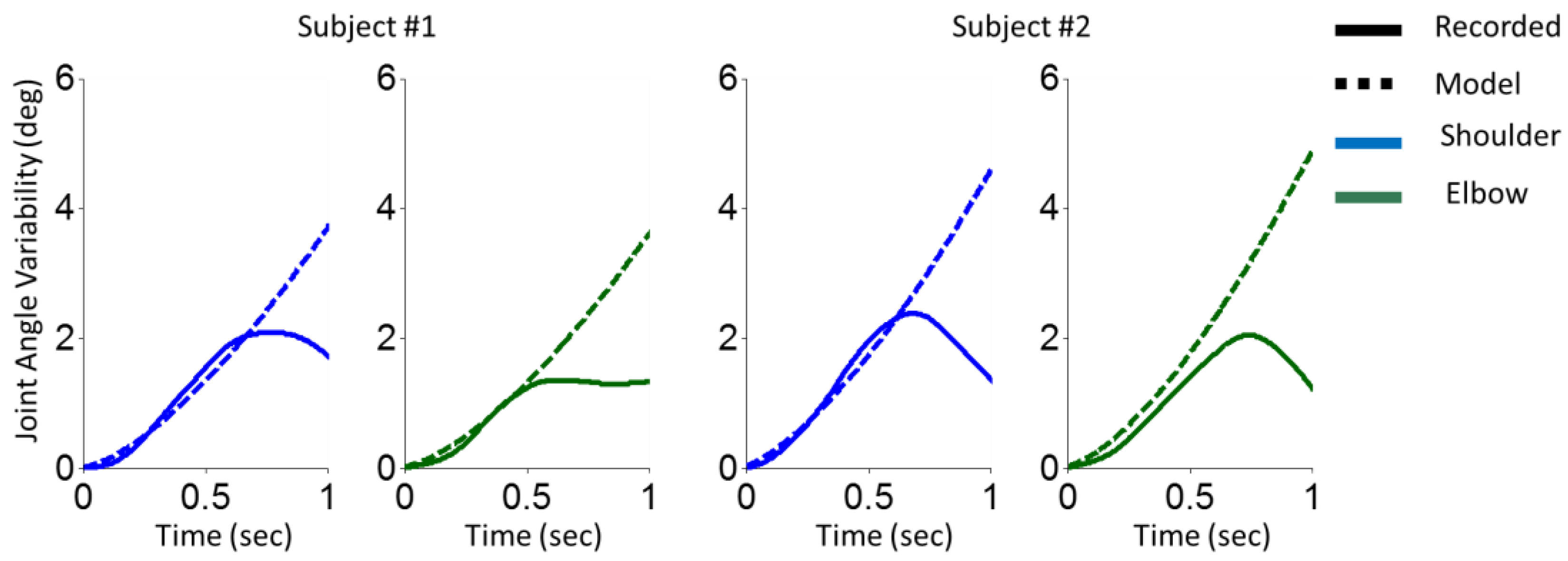
Figure 1. Variability of shoulder and elbow joint angles in an arm reaching movement task. The variability of shoulder (blue) and elbow (green) joint angles of two participants corresponding to recorded data (solid line) and the model (dashed line) are illustrated. Two left columns are for the first participant, and two right columns are for the second participant.

Figure 2. Variability of shoulder and elbow joint angles in an arm reaching movement task. The variability of shoulder (blue) and elbow (green) joint angles of two participants corresponding to recorded data (solid line) and the model (dashed line) are illustrated. Two left columns are for the first participant, and two right columns are for the second participant.

Figure 3. Variability of knee and hip joint angles in STS transfer. The variability of knee (blue) and hip (green) joint angles corresponding to recorded data (solid line) and model (dashed line) are illustrated. The left column is for the first participant, and the right column is for the second participant.

Disclaimer/Publisher’s Note: The statements, opinions and data contained in all publications are solely those of the individual author(s) and contributor(s) and not of MDPI and/or the editor(s). MDPI and/or the editor(s) disclaim responsibility for any injury to people or property resulting from any ideas, methods, instructions or products referred to in the content.

© 2023 by the authors. Licensee MDPI, Basel, Switzerland. This article is an open access article distributed under the terms and conditions of the Creative Commons Attribution (CC BY) license (http://creativecommons.org/licenses/by/4.0/).

Copyright: This open access article is published under a Creative Commons CC BY 4.0 license, which permit the free download, distribution, and reuse, provided that the author and preprint are cited in any reuse.

MDPI Initiatives

Important Links

Choose an area of interest and we will send you notifications of new preprints at your preferred frequency.

Disclaimer

Human Movements Are Shaped by Utilizing Sensory Information: A Stochastic Optimum Model

Abstract

Introduction

Methods and Materials

Results

Discussion and conclusion

Acknowledgments

Appendix A

Appendix B

Appendix C

References

MDPI Initiatives

Important Links

Subscribe