Predictive Models for Dissolved Oxygen in an Urban Lake by Regression Analysis and Artificial Neural Network

The paper portrays predictive models for dissolved oxygen (DO) levels in an urban lake using common water quality parameters like Temperature, pH, Conductivity and ORP at a time. Data were sampled using three real-time, industry-standard sensors, OPTOD, CTZN, and PHEHT, and then interpolated using the ArcGIS kriging technique. Correlation studies were analyzed through the ML algorithm, the correlation study signified a highly positive correlation between DO and other water parameters and the model was corroborated by R-score in order to create the linear regression model. In addition, an artificial neural network- a machine learning method using the Levenberg-Marquardt algorithm was developed to build a model to predict the do as well. Then, the performance of the models was validated and also the R² accuracy was checked of the predicted data against the actual data. Thus, the appropriateness of the ANN model for the forecasting of investigated attributes is indicated by the fact that the discrepancy between the forecasted and real ANN model is significantly lesser than that of the regression model. However, the model can be used to reveal DO data from unknown urban lake water.

Keywords:

Subject: Environmental and Earth Sciences - Environmental Science

1. Introduction

The cleanliness of water is a treasured, beneficial, and influential area of concern in most countries. Additionally, urban reservoirs or freshwater resources are absolutely essential for ecosystem stability, precipitation collection, refilling groundwater, encouraging recreational activities, particularly in lake regions, and supplying water for emergency situations like firefighting and hazard avoidance (Filik Iscen et al., 2008). However, Urban lakes are degraded and rendered less useful for excessive consumption, untreated industrial waste disposal, irrigation, sports, and perhaps other uses due to societal factors and also for some geological processes(Carpenter et al., 1998). Again, unplanned development causes major issues for urban lakes. The consequence of overexploitation upon those waterbodies can indeed be significant because of their magnitude, volume, or stagnancy (Brönmark and Hansson, 2002). Therefore, given the importance of freshwater cleanliness for aquatic ecological integrity and water availability for sentient exposure, it appears to be absolutely necessary to assess surface-water conditions (Ouyang, 2005). The terminology water quality condition relates to the biological, chemical and physical characteristics of water as well as the essential components of a water body that determine how reliable it is for consumption (Dogan et al., 2009a).

Admittedly, owing to the sustainability of aquatic species depends on the water quality characteristic known as dissolved oxygen (DO). To evaluate surface water quality, routine observation of DO is a crucial factor. In reality, a variety of physical as well as chemical processes affect how much DO is present in a stream hidden by the facility with which DO is measured. Aquatic culture may perish due to low DO concentrations in the lowered oxygen plume (Vikal, 2009). Despite having numerous methods, the most accurate approach for quantifying DO in waterbodies is the Winkler mechanism. To reduce latency during sample acquisition and analysis that might result in a difference in the oxygen concentration, this multistep chemical procedure is carried out immediately on-site (Griffiths and Jackman, 1957). Likewise, tangible measurements of DO by an electrochemical reactivity using polarographic Clarke electrodes. Limitations among them are in both methods oxygen is consumed thus resulting in calibration drift, flow dependency as well as electrical interference (Carpenter, 1965; Misra and Fridovich, 1976). There comes the challenging part of monitoring DO in real-time. It has to be accurately calibrated and checked for drift, it has to work under the conditions that came with the instruction. Eventually, sensors sometimes fail to put the correct data instead it puts null data for the system. Consequently, numerous forecasting model has been developed for this reason. In the past decades, scientists and researchers have developed the process of conventional information analysis techniques, however, aren’t adequate to address the issue because a significant variety of factors impacting the aquatic environment and have complex linear-nonlinear relationships with the water quality index (WQI)(Singh et al., 2009).

However, Linear Predictive Models (LPMs) and machine learning techniques have been widely used in environmental monitoring to forecast future trends, identify patterns and correlations, and detect anomalies in environmental variables (Hino et al., 2018). LPMs are mathematical models that use a set of input variables to predict an output variable. It is called linear because they make the assumption that the relationship between the inputs and outputs is linear (Vaseghi, 1996). In environmental monitoring, LPMs can be used to predict the future trends of various environmental variables (Berke, 1999). Machine learning techniques, on the other hand, are a set of algorithms and statistical models that enable computers to derive knowledge from data without explicit programming. It follows that, in environmental water quality monitoring, machine learning can be used for a wide range of tasks, such as classification (identifying the type of an environmental phenomenon, e.g., classifying water quality into different categories based on the concentration of various pollutants.), regression (predicting numerical values, e.g., prediction of the concentration of pollutants in water bodies based on historical data), and clustering (grouping similar instances together, e.g., real-time data from water quality sensors) (Tahmasebi et al., 2020).

Water quality models are very essential strategies that are created by merging data from several origins together into a model. The created model aids and improves awareness of the authorities and conventional water consumers’ concerns regarding the problems as well as the health of the water for consideration. Both affluent and developing nations are being impacted by the rising contamination levels in numerous water bodies. The discovery of untapped environmental resources for the purpose of the socioeconomic expansion is one of the main drivers of such an environmental problem (Gibbs, 1972). On the contrary, several scholars have recently conducted investigations in this regard to comprehend and model the phenomenon(Aziz-ur-Rahman and Muhammad, 2014; Dogan et al., 2009b; Gholizadeh et al., 2016; Wang et al., 2003). And also utilizing principal component analysis plus multiple linear regressions, Adamu and Ado conducted a study to pinpoint the origins of contamination and its associated role in the variance in water conditions (A. Mustapha and A. Abdu, 2012).

The major objective of this research is to construct water condition forecasting models which will be contrasted and investigated. Using common water quality parameters and pinpoint aspects and accuracy specifically related to researching a model to predict DO in Hahitjheel Lake, Gulshan, Bangladesh. However, in order to anticipate the DO, water quality data were examined statistically using multilinear regression critical analysis as well as artificial neural networks. The link between the water quality metrics is best represented by linear regression and ANN modelling has the ability to minimize time complexity, labour, and the chance of inaccurate measurements.

However, the current study has been done with the objectives;

i.: To assess the present pollution level using the fundamental water quality parameters and;
i.: ii. To develop predictive models for DO by regression analysis and artificial neural network.

2. Materials and Methods

2.1. Study Area

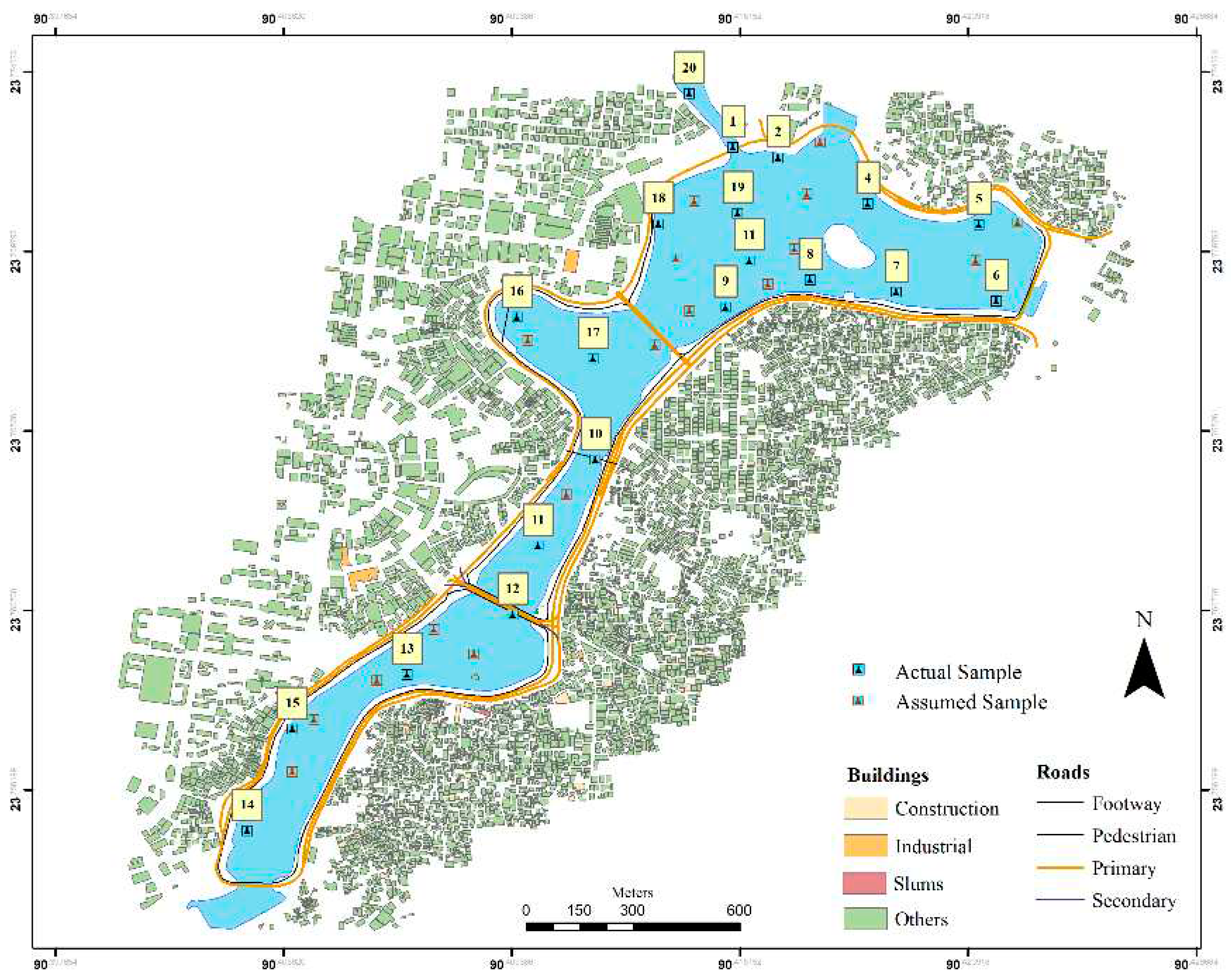
Hatirjheel lies in the center of Dhaka, the national capital city. Hatirjheel has geo-coordination of 23°44′58.47′′N and 90°23′48.35′′E. This region stretches between Pan Pacific Hotels and Resorts on the southern side through Banasree on the northern. The region seems to have a border with Tejgaon industrial region, Gulshan residential region, Rampura, Banasree, Niketon, Badda as well as Maghbazar, making commuting for residents of such sectors convenient (Mokaddes et al., 2013). Hatirjheel has covered a total space of 311.79 acres. Three significant streams border the region of Dhaka. However, throughout the wet seasons, the backwater movement of water from these streams floods the city’s outskirts, congesting the sewage system inside the city’s core. A few of the main sewage canals that convey stormwater runoff across catchments within eastern and central Dhaka towards the Balu River are the Begunbari canal and Banasree canal (Rahaman et al., 2017). Thus, the canal’s crucial hydrological role in emptying and containing rainwater from Dhaka metropolis’s vast expanse is very well acknowledged. The rainwater sewers that discharge into Hatirjheel are intended to convey rainwater but also transport dry weather circulation. Admittedly, among the few surviving large bodies of water inside Dhaka seems to be Gulshan Lake, which is significant both for the sustainability of the local environment and as a potential source of aquifer supply (Afrin et al., 2016).

Figure 1. Map of the study area and sampling points.

2.2. Data Collection and Sampling Procedure

The sample was collected from 20 sites on a random basis method of the ArcGIS software technologies. 16th of march 2022 was the sampling date and the timestamp mark was between 16.00 and 18.30. pH, salinity, temperature, redox and conductivity and DO (dissolve oxygen) parameters of the water quality were logged with the ML-317 ADS data logger and the CTZN: Inductive conductivity sensor for salinity, conductivity and temperature data, the OPTOD: Optical sensor for dissolved oxygen and the PHEH sensor for pH, Oxidation-Reduction Potential (ORP) was used. For every 5 seconds interval, the raw data was logged for each of the parameters for every 20 sites for 3 minutes. Through the process, 30 to 36 raw data were collected for each sampling site and for each of the six parameters.

2.3. Description of the Materials

The sensors used for the study to retrieve the water quality parameters were described in their manners. 1. AQUALABO’s CTZN: the method it uses is an inductive conductivity regulated in temperature and has an accuracy of ± 0.5 °C, 2. The OPTOD: Optical sensor, uses the method of optical measure by luminescence, which has an accuracy of ± 0,1 ppm, 3. The PHEHT: uses the method of the combined electrode (pH/ref), special glass and Ag/AgCI ref. gelled electrolyte (KCI) has the accuracy of ± 0,1 pH, ± 2 mV for ORP, ± 0,5 °C for temperature. However, these sensors’ data were combined and logged through the data logger YDOC’s ML-317 ADS using SDI-12 protocol and a storage device/memory card.

Figure 2. Real-time data collection framework.

2.4. Data Cleaning

Collected data needs cleaning and filtering for precise examination. In the process of data cleaning and filtering null values machine learning algorithm has been used. It was coded that if the null value is true and found algorithm has to put the mean value instead of the null value. Besides the corrupted, incorrect and incorrectly formatted data were removed for the clean analysis.

2.5. Study of Predictive Model

Regression models: As a way of modelling one parameter using multiple parameters regression model is among the best practices. The model uses the dependent and independent variables and then the correlation coefficient is the put-forward analysis to identify the nearness of the two variables. -1 to +1 of the correlation coefficient signifies the linear relationship between X and Y. However, the association is described as compelling throughout +0.8 to 1.0 as well as 0.8 to 1.0, intermediate throughout +0.5 to 0.8 and 0.5 to 0.8, and indecisive throughout +0.0 to 0.5 and 0.0 to 0.5. based on the relationship between the variables the model predicts or forecasts. On the contrary, the study tries to find the relationship between water quality parameters as input, X and model DO as Y by the given formula by Karl Pearson,

Y = β0 + β1X + ε

(1)

Where Y and X are respectively the dependent and the independent variable, β0 is the intercept while β1 is the slope or coefficient of the independent variable, and ε is the error term.

The resulting model makes predictions about the value of the dependent variable for new values of the independent variables. In this study, the change of one water condition indicator, which is the dependent variable, depends on multiple independent variables. The fundamental formula is:

Y = β0 + β1X1 + β2X2 + ... + βpXp + ε

(2)

where Y is the dependent variable, X1, X2, ..., Xp are the independent variables, β0, β1, β2, ..., βp are the coefficients or parameters that describe the relationship between the variables, and ε is the error term that represents the unexplained variation in the dependent variable. The goal is to enhance the association between the forecasted value of our water condition variable and the real value of the measure by selecting ideal independent variables.

Neural Network Models: An artificial neural network (ANN) is a type of machine learning algorithm inspired by the structure and function of the human brain. It is a network of interconnected nodes, called neurons, that work together to perform a specific task. In an ANN, the neurons are organized into layers, with each layer performing a specific function. The input layer receives the data, and the output layer produces the final output. The layers in between are called hidden layers, and they perform intermediate computations to transform the input into the desired output. Each neuron in an ANN is connected to other neurons through weighted connections. The weights represent the strength of the connection between the neurons, and they are adjusted during the training process to improve the accuracy of the model. During training, the ANN is fed with input data and the corresponding desired output, and the weights are adjusted to minimize the difference between the predicted output and the actual output. The total data of 20 samples from different sampling sites of Hatirjheel were used for building the model. Google’s Colaboratory is a product from Google Research that was used as IDE. For this research, the Levenberg Marquardt algorithm has been used and the code has been written in the python programming language.

3. Result and Discussion

3.1. Data Analysis

Collected and cleaned data from the 20 sampling sites were interpolated throughout the lake map using ArcGIS from ESRI for each of the parameters of water quality. These sample data were then verified and correlated among each other on a combination process to see if these data have a correlation with DO. All these processes were done using a machine learning algorithm for automation and for low latency temporal benefits using Python programming language. Now the sampled and interpolated data were generated into 30 more random values. A total of 50 values is now being constructed for further analysis. These 50 data merged into the equation of linear regression. The hypothesis is accumulated through a multiple regression equation that if one has the four of the parameters one might calculate through this machine learning method (sklearn, seaborn & matplotlib) and/or through the developed equation of multiple linear regression one can generate the unknown DO of the water.

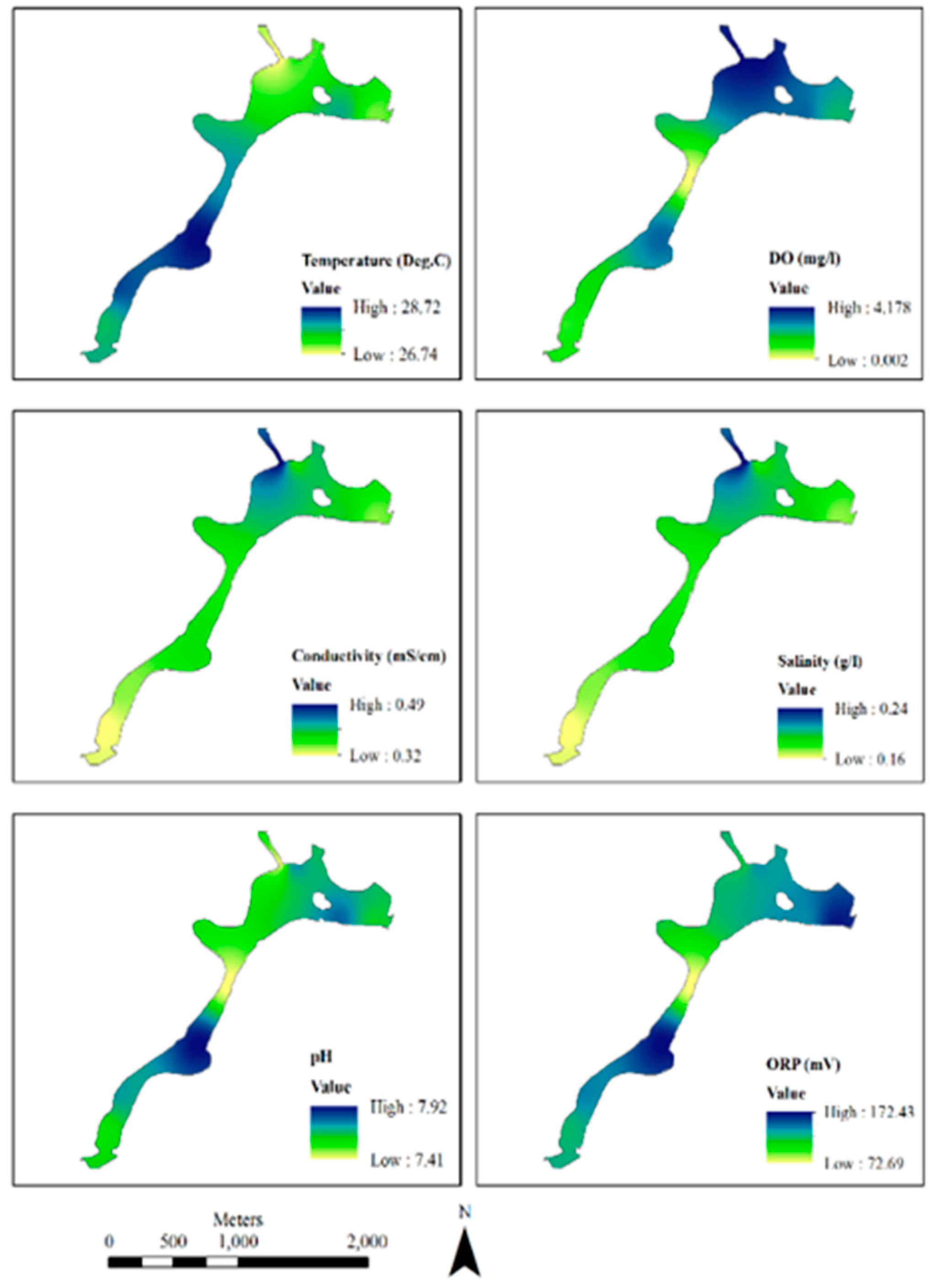
As shown in Figure 3, 20 samples were interpolated here from the original 20 observed values. The map represents the visible indication of an inverse relationship between pH value and DO. Again, among the other basic WQI parameters of the Hatirjheel lake. These maps were produced by ArcGIS from ESRI using the method of Kriging interpolation.

3.2. Mean and Standard Deviation

The below table indicates that the SD of DO and ORP from the dataset is much scattered and has shown significant deviation. The below data is shocking that the DO is very low from the standard level. This DO signify that the nutrients of the water are becoming absent and the water is not qualified for the fish culture. This prominent lake of Dhaka city has negative and almost no good for social benefits but is a mere tourist attraction.

Table 1. Mean and Standard Deviation of WQI data.

Sl.	Temp. (⁰C)		ORP (mV)		Salinity (g/l)		EC (mS/cm)		pH		DO (mg/l)
Sl.	Mean	SD	Mean	SD	Mean	SD	Mean	SD	Mean	SD	Mean	SD
1	28.72	0.14	115.47	1.23	0.24	0.00	0.49	0.00	7.43	0.02	0.00	0.00
2	28.72	0.15	138.71	2.23	0.19	0.02	0.37	0.04	7.75	0.03	1.03	0.40
3	28.37	0.08	138.89	4.72	0.20	0.01	0.39	0.02	7.70	0.02	1.48	0.24
4	28.02	0.07	153.93	3.48	0.19	0.01	0.37	0.03	7.67	0.02	1.34	0.19
5	27.77	0.04	168.56	1.12	0.18	0.03	0.35	0.06	7.62	0.02	0.81	0.08
6	28.28	0.03	141.44	4.96	0.19	0.00	0.39	0.00	7.80	0.01	2.44	0.08
7	28.31	0.08	137.13	5.19	0.20	0.01	0.39	0.02	7.70	0.02	1.67	0.30
8	28.19	0.09	127.39	5.00	0.20	0.01	0.40	0.02	7.63	0.02	1.52	0.60
9	26.74	0.09	72.70	19.20	0.18	0.00	0.36	0.00	7.41	0.01	2.78	1.65
10	28.43	0.09	130.43	4.20	0.20	0.01	0.41	0.02	7.63	0.02	1.15	0.39
11	27.77	0.07	138.08	8.22	0.19	0.01	0.37	0.02	7.74	0.02	3.50	0.72
12	28.28	0.06	172.43	2.48	0.19	0.00	0.38	0.00	7.92	0.02	4.18	0.10
13	27.74	0.06	147.62	4.65	0.18	0.01	0.36	0.03	7.76	0.02	3.44	0.05
14	27.15	0.04	124.26	1.08	0.17	0.03	0.33	0.06	7.57	0.02	2.11	0.16
15	27.42	0.03	143.90	4.97	0.18	0.02	0.35	0.03	7.73	0.03	3.54	0.13
16	27.66	0.09	113.54	6.27	0.19	0.01	0.38	0.02	7.58	0.02	2.25	0.82
17	27.38	0.08	101.01	9.99	0.19	0.01	0.38	0.02	7.53	0.02	2.41	1.10
18	28.43	0.10	124.86	4.04	0.21	0.01	0.43	0.02	7.58	0.02	0.97	0.39
19	28.60	0.10	128.02	3.03	0.21	0.01	0.43	0.02	7.60	0.02	0.75	0.29
20	28.63	0.10	123.35	3.14	0.22	0.01	0.45	0.02	7.54	0.02	0.50	0.15

* SD = Standard Deviation.

Water quality standard: Compared with the above table the data found in the study were nowhere relatable to the standard of WHO & DoE gave. According to World Health Organization (WHO)’s Guidelines for drinking water quality. Vol. 2, Health criteria and other supporting information, 2nd ed, water quality parameters are standardized in 1993 (World Health Organization., 1993). Table 2 for DO, ORP, salinity, pH, and EC are standards according to DoE, Gov. of Bangladesh also (Huq, 2003). The Department of Public Health Engineering, Gov. of Bangladesh also gave standard data (DPHE, n.d.) table on their website which is marginally similar to the data given by DoE.

3.3. Correlation Analysis

In statistics, correlation denotes the relationship of two numerical data. The relationship is linear, meaning that an operator increasing/decreasing in one operator causes a particular number increase/reduction in another.

R = \frac{Σ (x - ẋ) (y - ẏ)}{{\sqrt{[Σ (x - ẋ) (y - ẏ)]}}^{2}}

(3)

Where, r= the linear relationship between the x & y variable, x= values of x variable, ẋ= mean value of x variable, y= value of y variable, ẏ= mean value of y variable.

When checking the correlation among the other parameters it seemed that 25 correlations are found and among them, the top 5 correlated tables are given in Table 2. Table 2 indicates that the correlation with DO against pH, Salinity, Conductivity and temperature is higher in the result than with other parameters included like ORP. Then the score of R came 0.687. Also, the mean discrepancy between variables observed versus obtained variables is measured by RMSE. It gives an estimate of how well the model fits the accuracy. However, the score of RMSE is 0.834 which is quite a good score. Since, a lower value of RMSE indicates a better fit for the model.

On the other hand, correlation heat maps provide graphical representations of such intensity of correlations among quantitative data. Correlation maps are being utilized to determine which of them are related to another and how strong that association is. Figure 3 has given an insight into the relationship between the parameters taken into consideration in this research paper. As the graphical illustration, DO has a moderate correlation with pH and negative relation with temperature, conductivity and salinity.

3.4. Regression Model

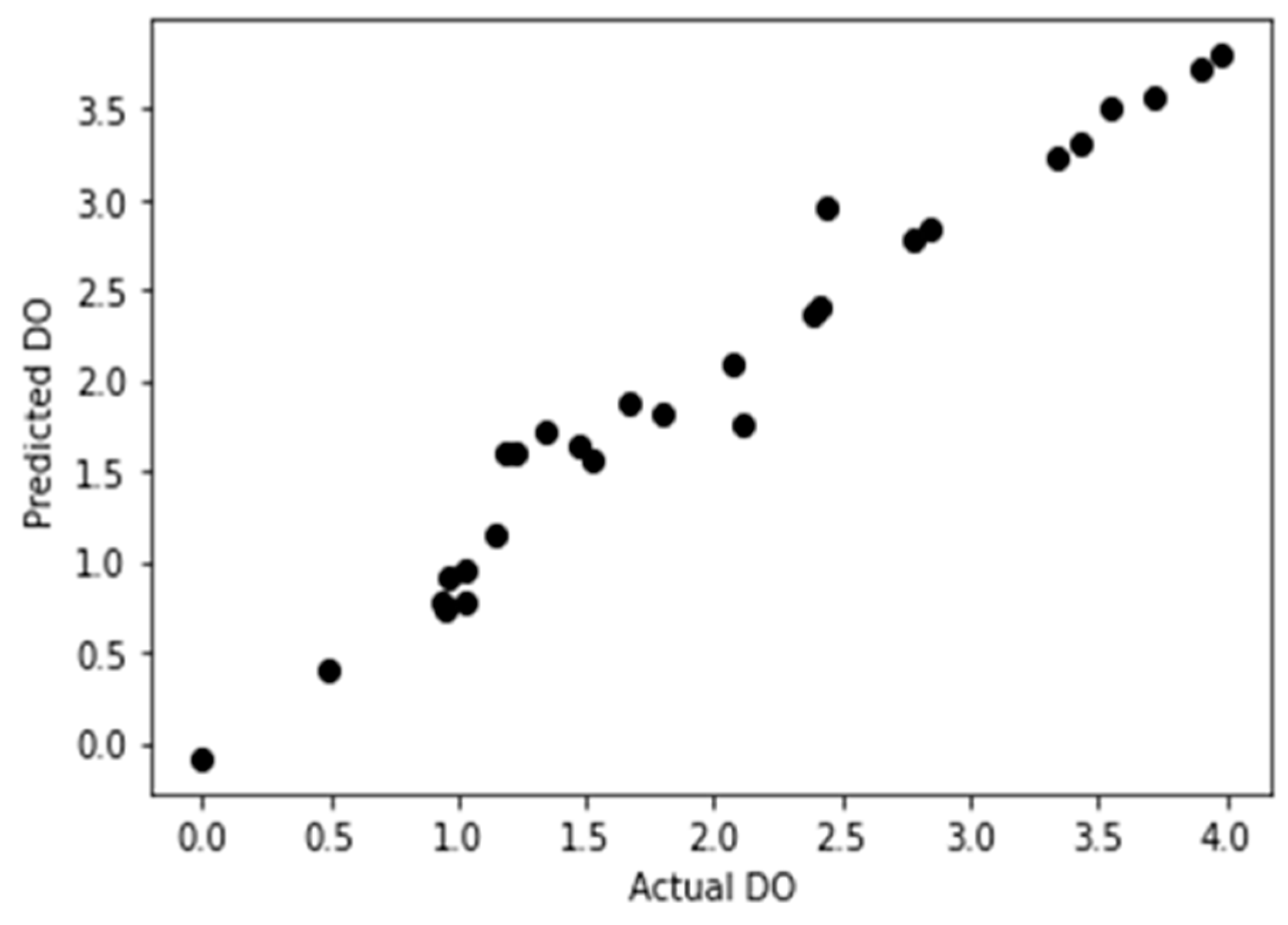
The DO prediction model using the four parameters of water quality developed through the machine learning method was used to produce the statistical results of the regression model. Where 40 total sample data were used. In the dataset 20 was original sampling and 20 was interpolated data. The model was trained in a way that the machine learning model itself used 70% of data as in 28 data for training the model and the rest 12 data kept to check if the model is valid. The accuracy of the model came in 0.96 which is a great fit for the model building and the equations RMSE (root-mean-square-error), MSE (mean squared error), and MAE (mean absolute error) was developed and the c=Intercept value also found.

Table 4. Statistical results of regression model.

Methods	Statistical values
r²	0.9636419890515832
MAE	0.15244809592781455
MSE	0.04297761323587285
RMSE	0.20731042722418197
Intercept	-3.243182537397614
Temperature coef.	-3.50012194
pH coef.	12.43320371
Salinity coef.	-315.35944705
Conductivity coef.	179.27832613

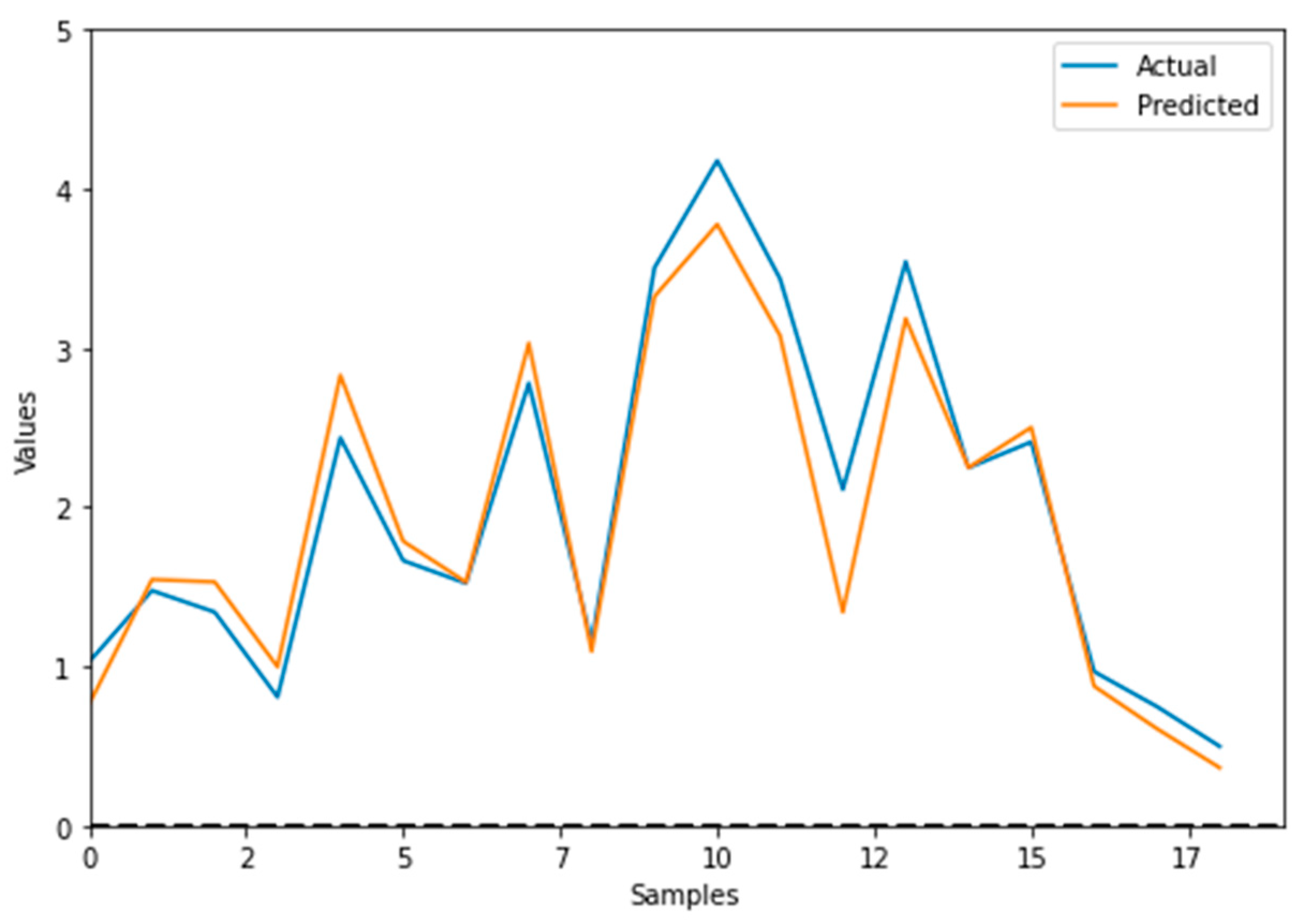
Regression Equation: Therefore, the equation of the regression stands as, Y (Predicted DO) = (-3.50012194 * Temperature) + (12.43320371 * pH) + (-315.35944705 * Salinity) + (179.27832613 * Conductivity)—3.243182537397614

As per the developed equation, the predicted DO and the actual DO stand in a curve like Figure 5.

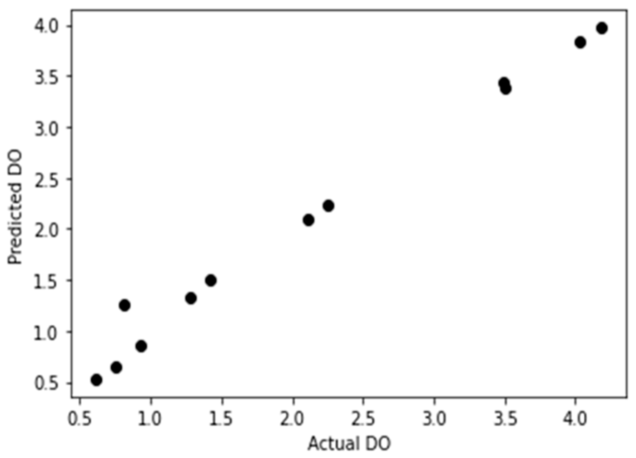
Model Validation: On the contrary, for the validation of the regression model the model was tested against those 12 data means 30% of the dataset and the result is given below,

Table 5. Statistical result of model validation.

Method	Values
r2	0.9830437024851376
MAE	0.12126691975959207
MSE	0.028476917606881477
RMSE	0.16875105216525754

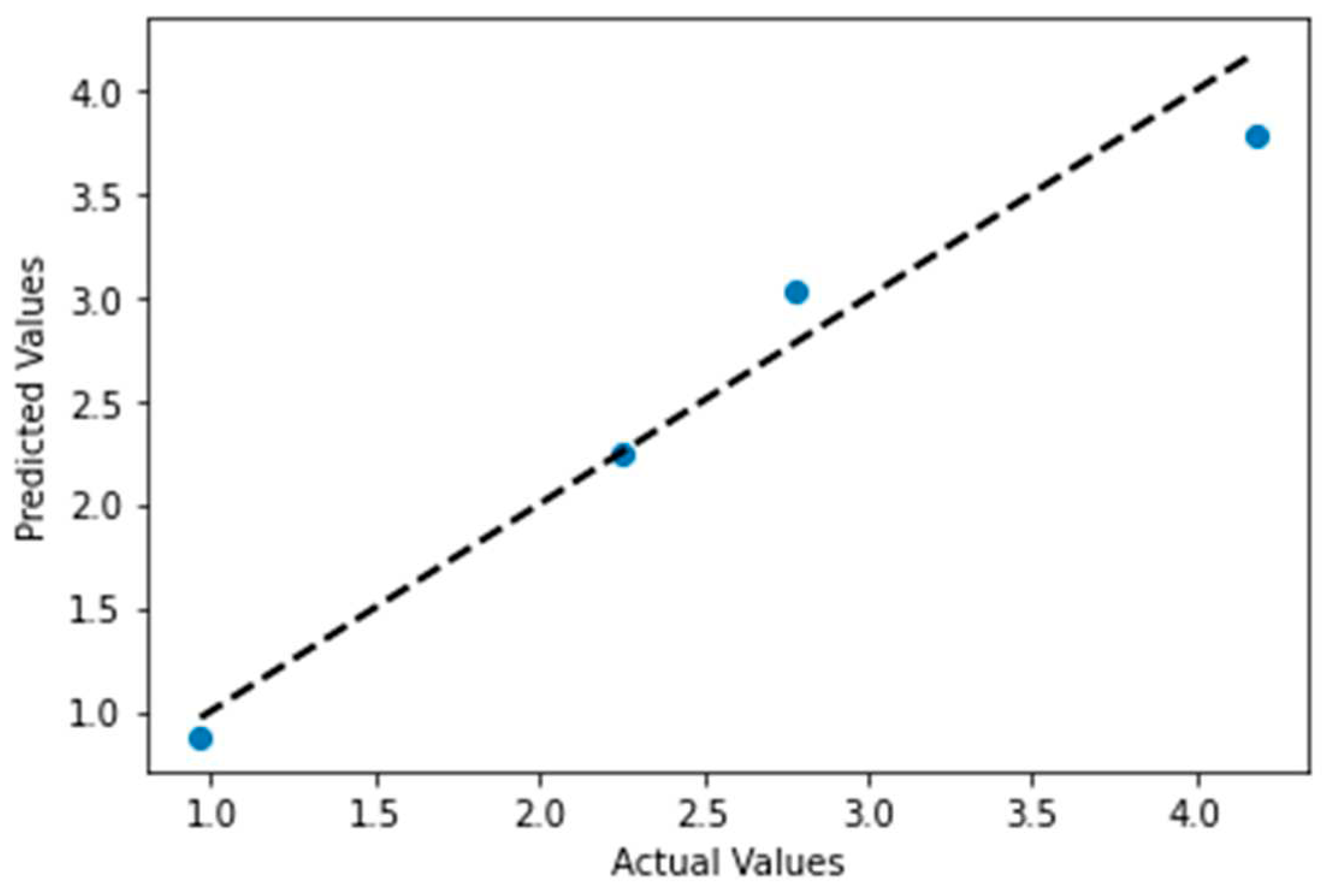
However, the simulation of the dissolved oxygen by linear regression predictive model accuracy curve was shown in Figure 6. Importing the 12-forecast sample data into the prediction model, the prediction result of r² is 0.963. This demonstrated a strong and effective proposed dissolved oxygen forecasting model.

3.5. Neural Network Model

In the current research, the Levenberg-Marquardt algorithm (LMA) was used to build a predictive model for the dataset. The dataset was split into three groups: 14 samples for training (70% of the data), 3 samples for testing (15% of the data), and 3 samples for validation (15% of the data). The model was built using Python programming language and implemented in Google Colab, a cloud-based development environment. We set the number of hidden layers to 10 to ensure sufficient complexity of the model. Our results show that the Levenberg algorithm was successful in predicting the outcome of the dataset, with a high degree of accuracy and reliability. The model was able to generalize well to new, unseen data, indicating its robustness and effectiveness.

However, model validation MSE: 0.05806477927606786, model validation r²: 0.9561864749339852, model testing MSE: 0.186e1912474875776 and model test r²: 0.8092677214484836 was the output of the ANN model and Figure 7 is the plotting of the validation curve.

Consequently, the ANN-developed model was used to predict and plot against the actual DO data the output curve shown in Figure 8. The model’s MSE was 0.0778092174395809 and r² came 0.9313023303847828. Figure 9, shows the infinite curve of the difference between the actual and predicted values generated by ANN. However, these findings suggest that the Levenberg algorithm is a valuable tool for predictive modelling in a variety of applications. Future studies may explore the potential of this algorithm in other domains and with larger datasets.

3.6. Assessment of the ANN Model and The Regression Model

For the purpose of determining whichever model (regression or ANN) represents the actual readings more precisely, the actual and predicted measurements of the DO are compared, and the evaluation table is shown in Table 6. The evaluation is done using actual data that was gathered during sampling using sensors. The predicted measurements using the ANN model plus regression were being contrasted with the actual data. Table 6 additionally displays the computed error for either the model for DO prediction. Table 6 shows that the ANN model better reflects the actual DO readings. From 0.00 to 54.15, the difference in error comparing the actual and calculated ANN models. Regression model error, meanwhile, spans from 0.04 to 56.87.

3.7. Limitations of the Study and Further Scope

The main and foremost limitation of the research is that the DO models are prepared using only a few basic water quality matrices, other parameters such as biological and chemical dissolve oxygen demand were not taken into consideration. Additionally, heavy metals like Cd, Cr, Ni, Arsenic and other significant ones were also not taken into consideration for this scientific study and remain for future scope. However, fish culture damage data due to DO decrease is also not taken under lab experiments and close system scientific simulator exploration. Furthermore, the models are not developed using time-series data and initially, it was decided that it needs to be done in a basic manner without complex data. Keeping in mind, the data as well as the models were kept simple and clean to understand easily. Therefore, as we haven’t, there is a high opportunity for further study in this particular idea module.

4. Conclusion

Correlation analysis and studies indicate a very significant correlation between DO and pH, temperature, salinity and conductivity. R of them found in 0.963 in Hatirjheel.
An abysmal correlation was found when ORP is taken under consideration with DO including other parameters.
Modelling of DO by ANN suggests a quite impressive correlation between the actual and predicted measurements. R² value came to 0.93. However, for model validation R² is 0.80.
ANN model is giving the best prediction values for DO. Although the error between the predicted and actual ranges from 0.00 to 54.15 and the error from the regression model came from 0.04 to 56.87. finally, it can be recapitulated that ANN might be an efficient model for modelling DO with the analyzed parameters.

Author Contributions

A. Selim:Conceptualization, Data collection, Validation, Formal analysis, S. N. A. Shuvo: Writing—original draft, Conceptualization Formal analysis. M. M. Islam: Writing-review & editing, Conceptualization. S. Shah: Software, Formal analysis. M. Ohiduzzaman: Arranging and reviewing the draft. M. Moniruzzaman: Final review and editing for submission.

Acknowledgments

The authors are highly grateful to Eutech Systems Limited, 155/A, Niketon, Gulshan-1, Dhaka, Bangladesh for all kinds of supports to conduct this research including providing the water sensors, data collection facilities, data analysis and associates economic costs.

Conflicts of Interest

The authors declare that they have no known competing financial interests or personal relationships that could have appeared to influence the work reported in this paper.

References

Mustapha, A. Abdu, 2012. Application of Principal Component Analysis & Multiple Regression Models in Surface Water Quality Assessment. Journal of environment and earth science 2.
Afrin, Sadia, Islam, Mohammad Maksimul, Rahman, Md Mujibur, Afrin, S, Islam, M M, Rahman, M M, 2016. 8 th International Perspective on Water Resources and the Environment Sri Lanka.
Aziz-ur-Rahman, Muhammad, O.C., 2014. Reginol interpretation of river Indus water quality data using regression model. Afr J Environ Sci Tech 8. [CrossRef]
Berke, O. , 1999. Estimation and prediction in the spatial linear model. Water Air Soil Pollut 110. [CrossRef]
Brönmark, C. , Hansson, L.A., 2002. Environmental issues in lakes and ponds: Current state and perspectives. Environ Conserv. [CrossRef]
Carpenter, J.H. , 1965. THE ACCURACY OF THE WINKLER METHOD FOR DISSOLVED OXYGEN ANALYSIS. Limnol Oceanogr 10. [CrossRef]
Carpenter, S.R. , Caraco, N.F., Correll, D.L., Howarth, R.W., Sharpley, A.N., Smith, V.H., 1998. Nonpoint pollution of surface waters with phosphorus and nitrogen. Ecological Applications 8. [CrossRef]
Dogan, E. , Sengorur, B., Koklu, R., 2009a. Modeling biological oxygen demand of the Melen River in Turkey using an artificial neural network technique. J Environ Manage 90. [CrossRef]
Dogan, E. , Sengorur, B., Koklu, R., 2009b. Modeling biological oxygen demand of the Melen River in Turkey using an artificial neural network technique. J Environ Manage 90. [CrossRef]
DPHE, n.d. Water Quality Parameters [WWW Document]. Bangladesh National Portal. URL http://dphe.gov.bd/site/page/15fa0d7b-11f1-45c0-a684-10a543376873/Water-Quality-Parameters- (accessed 2.22.23).
Filik Iscen, C. , Emiroglu, Ö., Ilhan, S., Arslan, N., Yilmaz, V., Ahiska, S., 2008. Application of multivariate statistical techniques in the assessment of surface water quality in Uluabat Lake, Turkey. Environ Monit Assess 144. [CrossRef]
Gholizadeh, M.H. , Melesse, A.M., Reddi, L., 2016. A comprehensive review on water quality parameters estimation using remote sensing techniques. Sensors (Switzerland). [CrossRef]
Gibbs, R.J. , 1972. Water chemistry of the Amazon River. Geochim Cosmochim Acta 36. [CrossRef]
Griffiths, V.S. , Jackman, M.I., 1957. The winkler method for dissolved oxygen determination. Anal Chim Acta 17. [CrossRef]
Hino, M. , Benami, E., Brooks, N., 2018. Machine learning for environmental monitoring. Nat Sustain 1. [CrossRef]
Huq, M. , 2003. Water Quality Standard, A Compilation of environmental laws of Bangladesh. Department of Environment (DoE), Govt. of Bangladesh.
Misra, H.P. , Fridovich, I., 1976. A convenient calibration of the Clark oxygen electrode. Anal Biochem 70. [CrossRef]
Mokaddes, M. , Nahar, B., Baten, M., 2013. Status of Heavy Metal Contaminations of Drain Water of Dhaka Metropolitan City. Journal of Environmental Science and Natural Resources 5. [CrossRef]
Ouyang, Y. , 2005. Evaluation of river water quality monitoring stations by principal component analysis. Water Res 39. [CrossRef]
Rahaman, M.M. , Rahman, M.H., Hashem, M.A., Islam, M.R., 2017. Design study of boat for gulshan-banani-hatirjheel lake in the capital city of Bangladesh, in: Procedia Engineering. [CrossRef]
Singh, K.P. , Basant, A., Malik, A., Jain, G., 2009. Artificial neural network modeling of the river water quality-A case study. Ecol Modell 220. [CrossRef]
Tahmasebi, P. , Kamrava, S., Bai, T., Sahimi, M., 2020. Machine learning in geo- and environmental sciences: From small to large scale. Adv Water Resour. [CrossRef]
Vaseghi, S. v. , 1996. Linear Prediction Models, in: Advanced Signal Processing and Digital Noise Reduction. [CrossRef]
Vikal, P. , 2009. Multivariant analysis of drinking water quality parameters of lake Pichhola in Udaipur, India. Biol Forum 1.
Wang, H. , Hondzo, M., Xu, C., Poole, V., Spacie, A., 2003. Dissolved oxygen dynamics of streams draining an urbanized and an agricultural catchment. Ecol Modell 160. [CrossRef]
World Health Organization., 1993. Guidelines for drinking-water quality. World Health Organization.

Figure 3. Interpolation of different WQI parameters.

Figure 4. Correlation Heat map of the parameters.

Figure 5. Predicted DO vs Actual DO by regression model.

Figure 6. Model validation curve (r² = 0.98).

Figure 7. Output of ANN, validation curve.

Figure 8. Output of ANN, Predicted DO vs Actual DO.

Figure 9. Actual value in contrast with the predicted value.

Table 2. Water quality standard according to WHO & DoE.

Parameters	Standard (WHO)	Standard (DoE)
DO	6.5–8 mg/L	6 mg/L
ORP	300–500 mV	-
Salinity	<0.5 ppt	0.6 ppt
pH	7–8	6.5–8.5
EC	500-1400 µ/cm	1200 µ/cm
Temp.	12–25 °C	-

Table 3. Correlation with DO against other parameters.

Variables used	R-score	RMSE
pH, Salinity, Conductivity, Temperature	0.687	0.834
pH, ORP, Salinity, Conductivity, Temperature	0.680	0.843
pH, Conductivity, Temperature	0.591	0.954
pH, Temperature	0.544	1.007
pH, ORP, Salinity, Conductivity	0.4368	1.119

Table 6. Comparison of regression and ANN model with predicted values.

Actual DO	Predicted DO		Error (%)
Actual DO	Regression DO	ANN (DO)	ANN	MLR
0.002543	0.002036667	0.002	21.35273299	19.91083704
1.028873	0.779054303	0.6928057	32.66363293	24.28080983
1.476761	1.635235917	1.59623493	8.0902685	10.73125013
1.341628	1.717853974	1.69042387	25.99795696	28.04249567
0.80749	1.266742013	1.24480746	54.15763167	56.87401857
2.437044	2.949984711	2.91524763	19.62228134	21.04765903
1.665083	1.874985648	1.84167314	10.60548573	12.60613725
1.522556	1.570938816	1.54836212	1.694920909	3.177736403
2.780289	2.781594626	2.80576767	0.916403654	0.046960076
1.150079	1.144736965	1.11426831	3.113759142	0.4644929
3.504549	3.38432269	3.36737612	3.914137882	3.430578643
4.17886	3.970392534	3.93100286	5.931214255	4.988620481
3.435496	3.304870413	3.29252467	4.161592096	3.802233705
2.111274	1.756949546	1.76734976	16.28989132	16.78249501
3.543671	3.501936392	3.50765826	1.016255177	1.177722419
2.248047	2.228162467	2.22346257	1.09359057	0.884524778
2.410704	2.406895922	2.41047993	0.009294795	0.157965387
0.967645	0.91223125	0.89529996	7.47640302	5.726661077
0.748045	0.646836225	0.61761923	17.43555134	13.52977096
0.498015	0.403179732	0.39374483	20.9371545	19.04265287

Disclaimer/Publisher’s Note: The statements, opinions and data contained in all publications are solely those of the individual author(s) and contributor(s) and not of MDPI and/or the editor(s). MDPI and/or the editor(s) disclaim responsibility for any injury to people or property resulting from any ideas, methods, instructions or products referred to in the content.

© 2023 by the authors. Licensee MDPI, Basel, Switzerland. This article is an open access article distributed under the terms and conditions of the Creative Commons Attribution (CC BY) license (http://creativecommons.org/licenses/by/4.0/).

Copyright: This open access article is published under a Creative Commons CC BY 4.0 license, which permit the free download, distribution, and reuse, provided that the author and preprint are cited in any reuse.

MDPI Initiatives

Important Links

Choose an area of interest and we will send you notifications of new preprints at your preferred frequency.

Disclaimer