1. Introduction
According to the World Health Organization (WHO), people born in 2015 will have an average life expectancy of 20 years longer than people born 50 years ago in most of the world. Thus, there is also an expansion in the incidence of pathologies inherent to aging with increased longevity. In this sense, people over 60 are usually affected by neurological diseases that cause tremors – oscillatory involuntary movements in some parts of the body [
1,
2].
Tremors can be classified as tremors in action and tremors at rest [
3]. Essential tremor (ET) is more predominantly action-related and affects the upper limbs, such as the hands and head, with frequency characteristics ranging from 4 Hz to 12 Hz [
4]. This type of tremor can be bilateral or symmetric [
5]. ET figures as one of the most prevalent neurological diseases in the world. Luis and Ferreira [
6] estimated that about 1% of the world’s population and approximately
% of people over 65 years of age suffer from ET. On the other hand, tremors at rest, in most cases, are related to Parkinson’s disease, which is the second principal pathology causing involuntary tremors. It occurs when the patient’s limb is completely relaxed and there is no anti-gravitational effort. In this case, unwanted movements are produced both in the lower limbs and in the upper limbs, in the frequency range between 3 Hz and 6 Hz [
5]. People who suffer from PD and ET have difficulties performing simple everyday tasks such as eating and writing [
5].
Conventional mitigating alternatives for these patients are linked to medication and surgical intervention. For treatment with the medication Levodopa, for example, it was observed that about 50% of patients, after 5 years of treatment, had some side effects such as agitation, hallucination, mood swings, and impulsivity [
7,
8], another form of treatment is surgical intervention.
Several devices have been developed in order to apply active, passive, and semi-active control techniques to help suppress unwanted movements arising from tremors, aiming to improve the life quality of people with PD and ET. Proportional, Integrative, and Derivative (PID) controllers have been used in recent research on vibration suppression, in which the controller act to minimize unwanted signal values in order to ensure that the system gain follows reference values [
9]. In the proposed analysis in [
10], for instance, a model of a human hand with four degrees of freedom was used, together with a piezoelectric actuator, showing the feasibility of using a PID controller to suppress PD vibrations. Such controllers can be fixed or can be updated according to some algorithm, such as adaptive techniques.
Our work brings a new contribution to discuss hand tremors suppression control with a comparison of adaptive techniques, more precisely Filtered-x based, for active vibration control applied to the suppression of movements arising from hand tremors. Among the advantages of the algorithms are faster convergence in ideal conditions and tracking capability. The comparisons account for complexity analysis, convergence time, and Mean Square Error (MSE) in the steady state. As is known, there are many challenges in research of this nature, especially in the difficulty of collecting and evaluating data on the intensity and frequency of tremors without the need to use invasive methods. In our analysis, we have used mathematical and computational models to analyze the attenuation effect. Therefore, tests in humans will not be considered in this study. The results presented in this work enable the performance analysis of the tested statistical learning algorithms involving Monte Carlo simulations.
The rest of this work is organized as follows. In
Section 2 the mathematical models used to represent the hand tremor signal are presented and discussed.
Section 3 presents the structure of the active vibration control and the filters used to compose the solution to the problem.
Section 5 presents the results, as well as a discussion of the findings. In
Section 6 final considerations and new directions for research in the area are presented.
1.1. Related publications
Active Vibration Control (AVC) consists of applying a force of opposite intensity to an external source of vibration. To reduce hand tremors, Turkistani [
11] developed a tremor suppression prototype consisting of a flexible, portable glove. This prototype has a micro-electro-mechanical vibration simulation module based on an accelerometer-gyroscope embedded in the glove that mimics hand vibration. The vibration signal is collected and sent to a microcontroller. So that it can be processed and the vibration motors present in the fingers are activated to reduce the tremor.
Another method to eliminate human arm tremors was developed by Chuanasa and Songscho [
12], who used the self-balancing technique. In this technique, a rotating unbalanced mass actuator was used to reproduce arm tremors with the same frequency range obtained from clinical sources. In addition to the composition of the counterbalance device designed to hold the dummy arm, a proportional derivative integral controller and an algorithm programmed in LabVIEW were used to control the rotary unbalanced mass actuator, anti-shaker, in the order to combat tremor.
The method used by Hosseini et al. [
13] consists of the mathematical modeling of a system with 4 degrees of freedom of a biomechanical system that represents the human hand. Active control is done by combining a proportional and derivative controller and tested, via MATLAB-Simulink, in three different types of actuators: piezoelectric, magnetic, and electric. Finally, the efficiency of each actuator was compared separately, with the piezoelectric actuator demonstrating greater efficiency in suppressing tremors such as those characteristics of Parkinson’s disease.
As can be seen in
Table 1, which presents a comparison of the techniques found in the literature that perform active vibration control, considering the last 7 years, there is no evidence that other publications have used adaptive filters to control vibrations associated to TE and PD. None of the techniques found showed signal acquisition.
2. Mathematical models of tremors in upper limbs
In this work, a mathematical model of hand tremor similar to signal patterns obtained by clinical means and mathematically validated is used. Thus, the need to acquire signals in humans is eliminated. There are also advantages of using mathematical models such as easy identification, good spectral frequency resolution, and convenient use in embedded systems.
2.1. Physiological tremor model by time series
The characterization method used by Jakubowski et al. [
16] in the distinction between essential, physiological, and parkinsonian tremors, consists of using higher-order statistics by Taylor series, in which third and fourth-order cumulants are implemented to describe the behavior of tremors. Furthermore, he claims that second-order Gaussian models are not able to distinguish between the three types of vibration patterns mentioned above.
The model presented by Zhang and Chu [
17] consists of the simulation of physiological tremors in an outstretched hand loaded with a weight of 2.3 to 4.5 kg, for 60 seconds, using an autoregressive model of order
, AR(3).
An autoregressive process of order
p, AR(
p), is given by:
where
are the model coefficients and
is a white noise with Gaussian distribution with zero mean and variance
. According to [
18] the order that will produce the smallest error is
.
2.2. Mathematical model of Parkinsonian tremor
Theoretically, the parkinsonian movement can be reconstituted by Fourier analysis with sinusoidal signals of multiple frequencies, where the amplitude and phase of the signal are determined by the spectrum [
18]. In such wise, a tremor signal
is given by,
in which
.
The collaboration of Reeke [
18], rests on a simple model, however very similar, to the real behavior of a vibration produced by the left wrist of a patient with Parkinson’s. These models are both described by the sum of two sinusoidal and by the multiplication of two sinusoidal frequencies different from those used in the sum.
The comparison in the time domain between the models by summing and sinusoidal multiplication by the real tremor recorded in a patient with resting tremor in the left wrist, in which sensors captured the supinator and patient’s wrist pronator. In the representation of [
18], it is possible to notice the accuracy of the mathematical model used and the representation in the frequency domain of the real tremor.
3. Vibration active control
Firstly, it is necessary to characterize the vibrational properties of the structure, i.e., to know how the parts of the structure vibrate, to understand and control the vibration. Thus, we enable anticipating vibration levels or determining the actions to control vibration. While passive noise control has been the predominant method used in tremor control applications, the search for ultimate vibration control has advanced to the extent that the use of active forces would be preferable to neutralize vibration. In this vibration control technic, called Active Vibration Control (AVC), the controller coefficients are constantly updated by an adaptive algorithm.
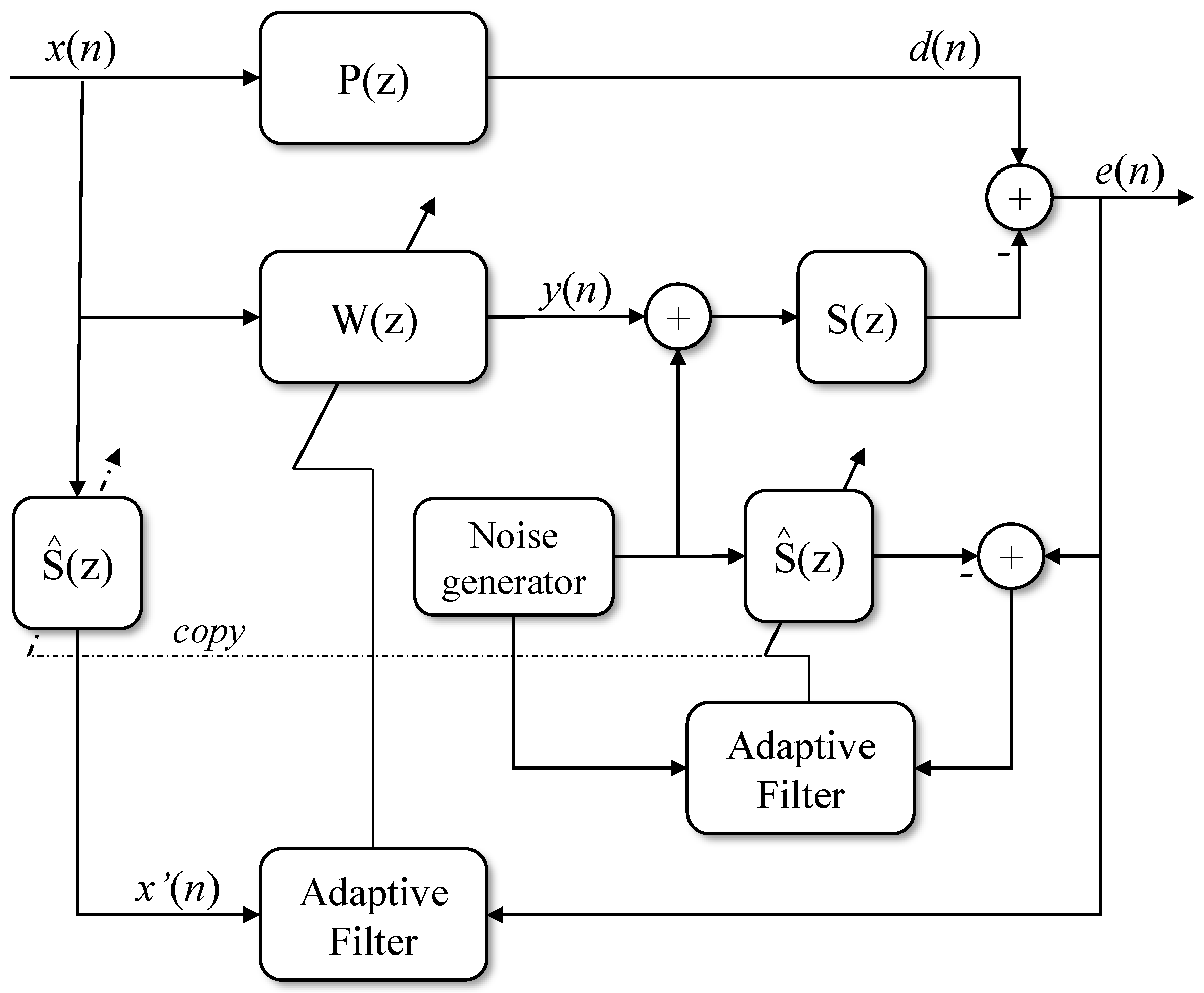
The AVC scheme, as highlighted in
Figure 1, basically consists of the plant system
1, actuators, sensors, and controllers. For the tests carried out, two random white Gaussian signals with zero mean and unit variance, uncorrelated, are generated. In
Figure 1 they are represented by the Noise Generator blocks and
. The signal
is used to recognize the plant coefficients of the main loop (direct path)
, on the other hand, the noise generator is an anti-signal generated in the loop (or secondary path) for recognizing the coefficients of the filter
. The response of the input signal into the second loop in a finite impulse response (FIR) filter is used to filter the
signal, which in turn feeds the adaptive algorithm, which acts to both recognize and estimate the coefficients of the main loop and to control the noise signal through the secondary loop.
Active vibration control based on adaptive finite impulse response (FIR) filters typically introduces a conditional signal dispersion delay [
19]. The reasons for these delays are geometric arrangements and computational time associated with the use of analog-to-digital converters (ADCs) and digital-to-analog converters (DACs). Delays represent a phase shift in periodic signals. These delays prevent instant feedback of signals from the Least-Mean Square (LMS) algorithm, for example. This can lead to instability and even divergence of the algorithms. Studies have presented a modification of the LMS algorithm, adjusting the underlying gradient descent algorithm [
20,
21,
22,
23] to work around this problem. The result is that any delays that occur can be fully compensated.
Different strategies are proposed for the use of the LMS algorithm in controlling noise and vibrations, usually taking into account that the LMS alone is not capable of attenuating unpredictable signals such as physiological tremors, for example. Active vibration control applications usually rely on the action of external elements, especially the analog-to-digital and digital-to-analog conversion processes, called here secondary path. In the presence of that processes, traditional algorithms such as LMS or RLS (Recursive Least Square), should not be applied, being the solution to this problem lying in filtering the input signal, using an estimation of the secondary path. The Filtered-x Least Mean Square (Fx-LMS) and its variations, which serve as the basis for this analysis, was an alternative proposed by Widrow et al. [
24]. The strategy adopted also in [
15] uses the Internal Model Control method (IMC
2), together with the Fx-LMS algorithm to suppress noise and vibrations. Its results show robustness and segment of reference values.
In this work, some adaptive algorithms based on the least mean squares for active control of variable vibration systems will be evaluated. The framework also uses an auxiliary filter to improve the online estimation of the secondary path. The secondary path is represented by the transfer functions of the auxiliary filter and the controller, and its Finite Impulse Response (FIR) model is also estimated with an adaptive strategy.
3.1. Adaptive algorithms
The definition of an adaptive automaton, according to Widrow [
25], consists of a system whose structure is adjustable in such a way that, based on a desirable value, its performance improves according to its contact with the applied environment. Thus, adaptive algorithms are employed where there is a constant change in their environment. They are usually applied in real-time systems, requiring a minimum calculation ratio per sample. These algorithms have a measurement process in order to get closer to the desired value. According to Aslam et al. [
23] and Nascimento and Silva [
26], adaptive filters can be seen as a disaggregating algorithm for mixing two signals and, for that, the reference values of one of the signals are essential.
3.1.1. Least-Mean Square (LMS) Algorithm
The Least Mean Square (LMS) algorithm is one of the most commonly used adaptive filtering algorithms due to its computational simplicity, ease of proving its efficiency in stationary environments, stable behavior when implemented with finite arithmetic precision, and because it does not need to estimate the approximation gradient of values offline [
25,
27]. The use of adaptive learning algorithms with statistical inference allows for estimating the behavior of systems that present characteristics that can change over time, as is the case of signals from hand tremors.
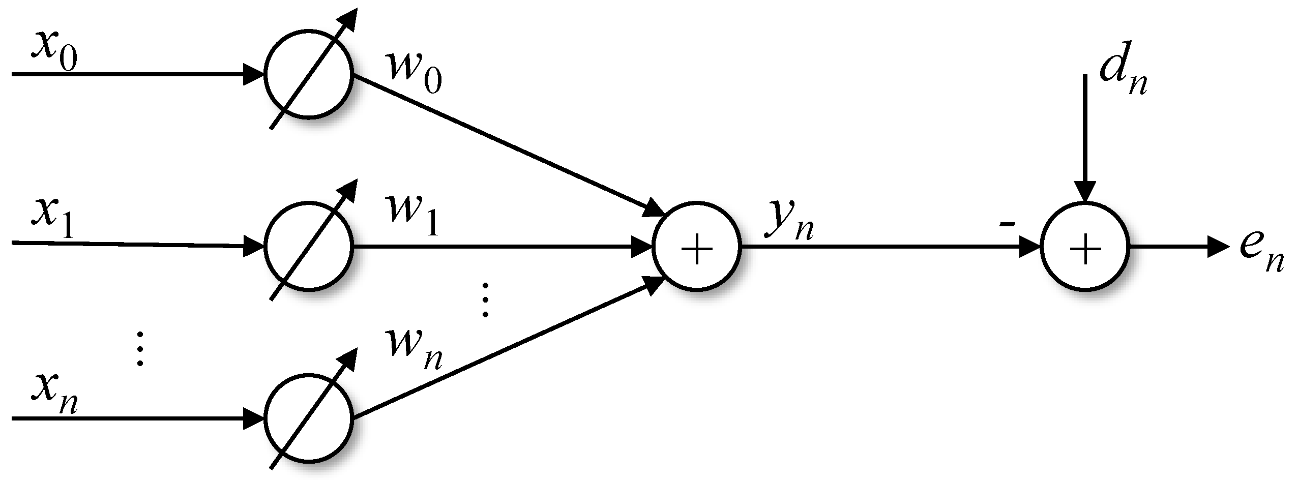
Figure 2, shows a diagram that helps in understanding the LMS. The vector
represents the system input values, the vector
refers to to the weights of the algorithm, which will be updated at each iteration,
represents the output estimated by the weights and the input by:
The signal is the signal to be approximated by the output of the system and represents the value of the error at instant n.
Taking the square value of the error (
5) in order to minimize it, yields:
The Mean Square Error (MSE) is obtained from the calculation of the mean operator,
, in (
6),
or
where
is the cross-correlation vector of input and output signals and
, known as the deterministic autocorrelation matrix of the input signal.
It is observed that from (
8), the MSE is given as a function of the weights, so the weights must be adjusted to reduce the error. This weight adjustment falls on a negative gradient in the decay rate of the root mean square error with respect to the weight adjustment, as shown by applying the derivative to (
7):
and
Substituting Equation (
5) into Equation (
10), we have:
The matrix
is a positive definite matrix and the solution,
, which minimizes the MSE, commonly known as the Wiener solution is given by:
The weight update equation for the LMS algorithm is given by:
where
is the adaptation step of the algorithm. The smaller this adjustment the more precise the adaptation, however a very small value of
can result in a slower response of the adaptation system due to the high number of points.
Substituting the values of (
11) in (
13) yields:
3.1.2. Normalized Least Mean Square (NLMS) Algorithm
The Normalized Least Mean Square (NLMS) Algorithm is a variation of the conventional LMS. In the LMS, the value of the learning step
is a fixed value, while in the NLMS this value is variable over time, in the form
[
28].
Thus, in the case of NLMS, (
14) can be rewritten as:
It is then necessary to define the posterior error since the adaptive step value is variable. Thus
and substituting (
15) into (
16), yields:
The value of
, which approximates the error value to its minimum, is given by:
in which
is the
-norm, i.e.,
Replacing (
18) in (
15), yields
Expression (
19) leads to an important regulation to determine the variation of the instantaneous squared error.
Now, let us introduce a positive real scaling factor
in (
18) in the same way of [
29]. This scaling factor is important to control the change in the tap-weight vector from one interaction to the next without changing the direction of the vector. Hence, the updating weights in the NLMS is given by:
Thus, we have a rate of convergence that is potentially faster than that of the LMS. Let us denote
by
from this moment for simplification.
3.1.3. Filtered-X Least Mean Square (Fx-LMS) Algorithm
For real-time active noise control applications, the LMS algorithm, due to the long delay, is not the most suitable algorithm, as the noise at the system input can generate instability. As an alternative to this problem, Widrow [
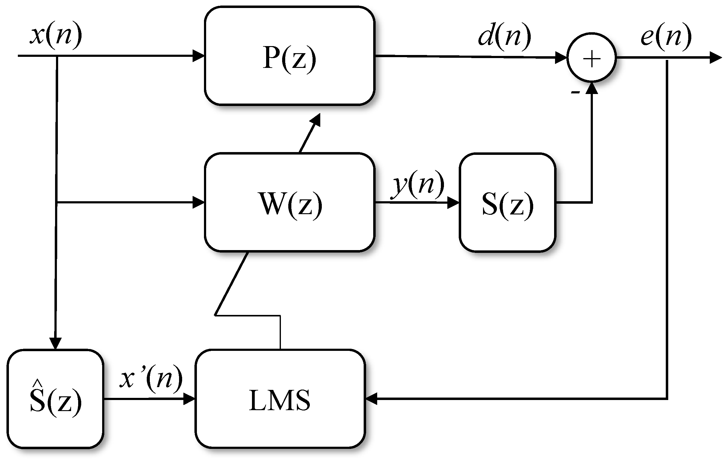
24] presented as a solution an algorithm that has an estimated signal input, in which the reference signal is adaptively filtered and compared with the input signal, obtaining the estimated signal. The Fx-LMS algorithm is normally used to update the adaptive filter, as shown in
Figure 3.
Analysis of the Fx-LMS convergence with stochastic signals on entry is presented in [
30] considering a moving average process. In this case,
is the primary path plan, and
represents the estimated value of
, its secondary path plan. Thus, the estimate of
is given by:
The equation that represents the error of the system, in the time domain, can be described as:
Assuming the output
, as well as in (
5), substituting in (
23), you get an error equation:
Using a methodology analogous to Wiener’s optimal solution, an expression similar to (
12) is obtained, but with filtered values, given by:
where
denotes the optimal vector of weights,
denotes the correlation matrix of filtered entries, and
represents the cross-correlation between the filtered input and the desired signal.
The expression for the input
is obtained by filtering
using
:
The optimal value of the error measured by substituting (
25) and (
26) in (
24), is given by:
From (
27) the weight vector that updates the Fx-LMS algorithm is:
where
, as in the LMS, is the convergence step of the algorithm.
4. Simulation configurations
In this section, simulation configurations are presented for comparison of adaptive algorithms to control tremors in upper limbs. The Fx-LMS and its variations, which serve as the basis for this analysis, was an alternative to solve the problem of traditional algorithms such as LMS and RLS [
24].
Based on the results, it is possible to analyze the behavior of the Fx-LMS and Fx-NLMS algorithms in the control of physiological tremors in a mesh that considers the online adjustment of the secondary path, eliminating the need for a fitting step during the calibration period. In addition, considering the characteristics of these algorithms, the behavior for a hybrid approach is also evaluated, being titled Fx-LMS&NLMS. This is a suggestion of changing the traditional format of the algorithms mentioned above.
In a second approach, control is applied to Parkinson’s tremors. In this case, the behavior of the Fx-LMS algorithm with sinusoidal input was considered, which will be denoted by Fsinx-LMS, an algorithm that is also a suggestion and adaptation of this analysis.
The design parameters (step-sizes) were defined by exhaustive trials, considering a faster fit for the secondary path for both controllers. The following value ranges were analyzed: to in steps of .
4.1. Simulation setup for physiological tremors control
The model used to simulate physiological tremors in this work is based on the study by Zhang and Chu [
17], in which the weight coefficients of the model described by an AR process were obtained through filtering by the Levinson-Durbin algorithm
3, presented in
2.1. The analysis of the algorithm was performed by the minimum MSE, which presented a residual error of
for a model of the third order.
The coefficients used in the AR(3) model to reproduce physiological tremor were
. To control the physiological tremors signal, the
plant must be a model proportional to
, in this work we have used
. A white Gaussian signal, with zero mean and unitary variance, was used to produce the desired signal
shown in
Figure 1.
The convergence step of the analyzed algorithms was maintained for all algorithms, as well as the number of interactions. After exhaustive tests, it was decided to use in the direct path and in the secondary path. In this way, the best results were obtained for both algorithms and scenarios.
4.2. Simulation setup for pathological tremors control
The model defined in
Section 2.2, Eq. (
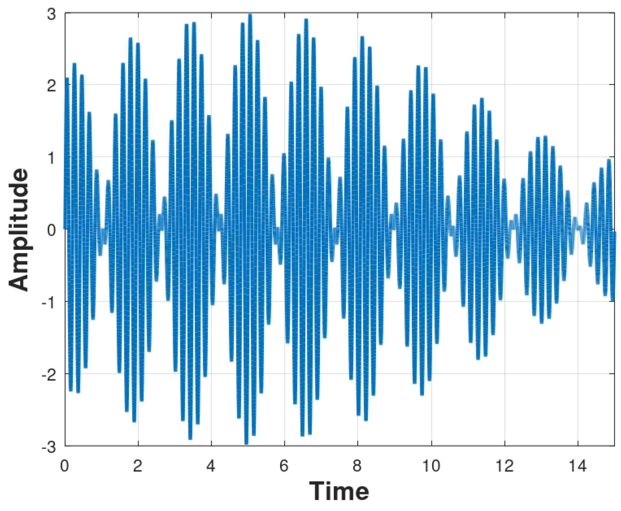
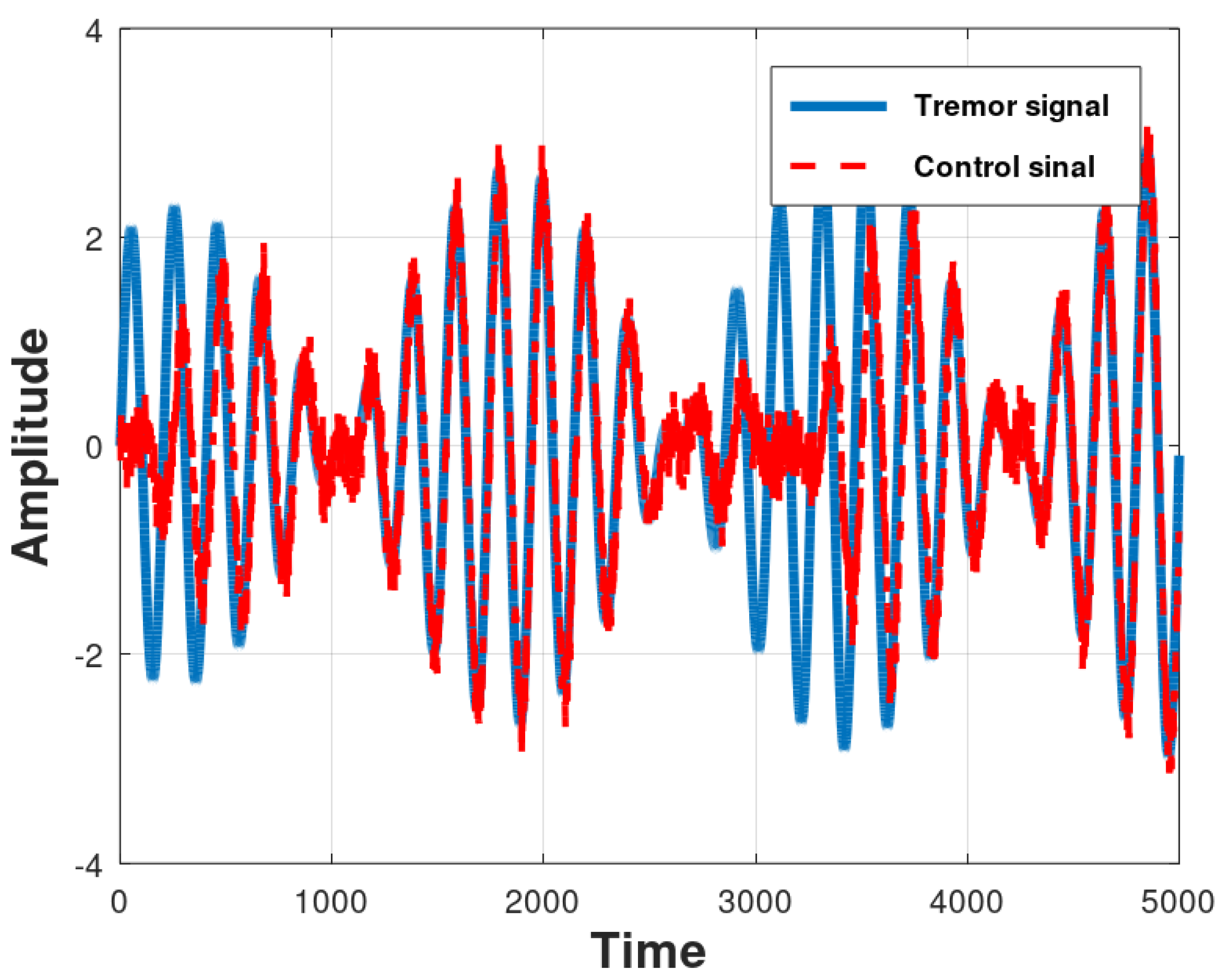
2) – which is a synthetic signal similar to Parkinson’s tremor – was used in order to generate the synthetic signal. This signal simulates the tremor of Parkinson’s disease, as can be seen in
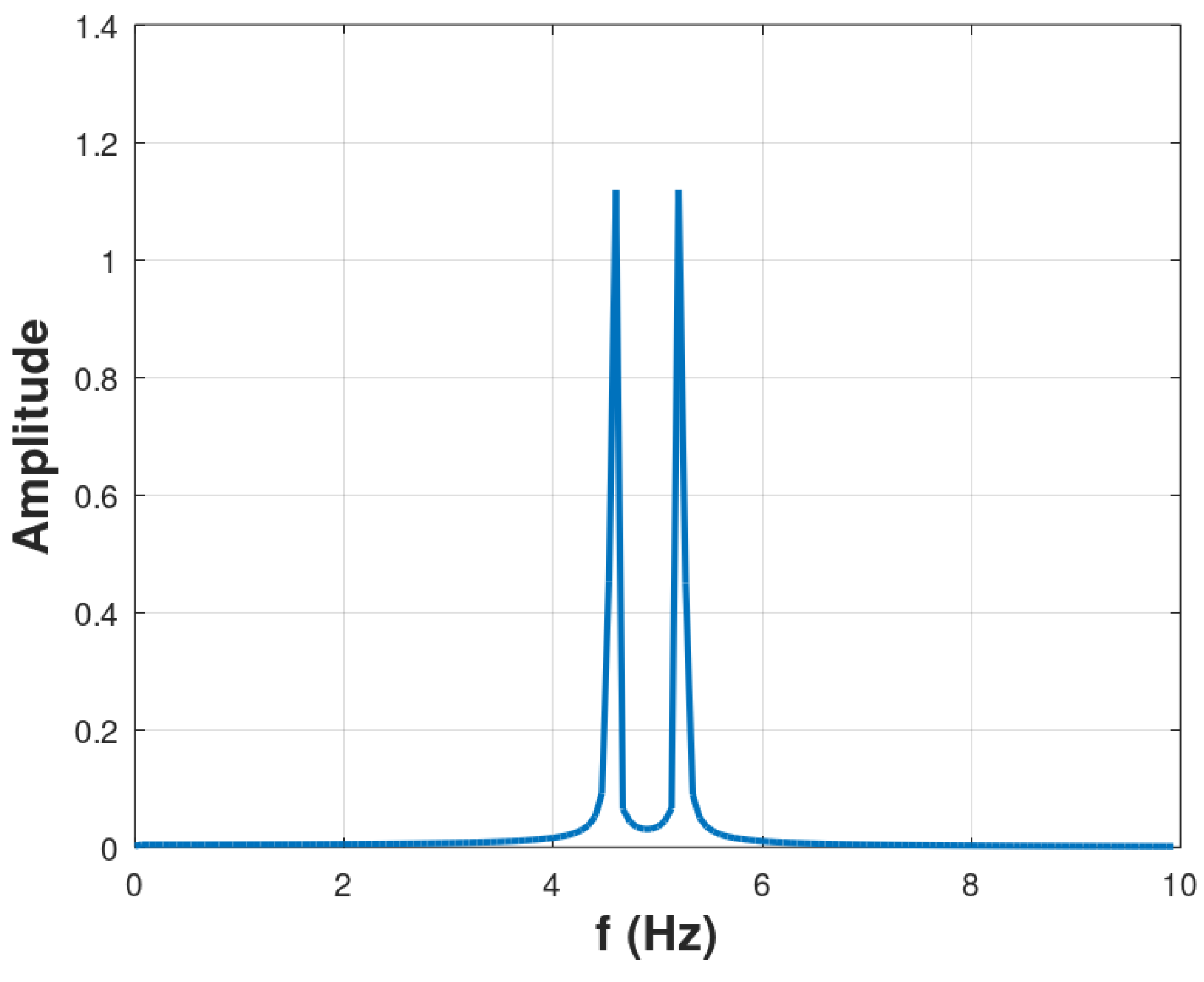
Figure 4. The frequency values used for the sinusoid sum were 5.2 Hz and 4.6 Hz.
Figure 5 represents the Fourier transform of the synthetic Parkinson’s tremor signal shown in
Figure 4. Note the occurrence of the peaks at approximately 4.5 Hz and 5.5 Hz.
Unlike linear systems which can be uniquely identified by their impulse response, nonlinear systems need to additional steps. In this way, we require nonlinear processing. Therefore, we need a transformation in input space to guarantee the modeling of the nonlinear part of the system.
The linear filter is
. The desired signal
was generated according (
2). The input signal
is the white Gaussian noise transformed by sinusoids. We clarify that, in this case, P(z) is not displayed because it is a non-linear system composed of the sum of sinusoids. The need to change the signals of the primary and secondary paths by sinusoids was due to the nonlinear characteristic of the desired signal
. This is an adaptation, called here the FsinX-LMS algorithm, given that the dynamics of the Parkinson’s disease signal are non-linear and deterministic. A Gaussian white noise generator would not be able to generate a control signal for Parkinson’s tremors, given its linear nature. We have used the step-size,
in the primary path and
in the secondary path.
5. Results
This section presents the reporting of the results of the experiments performed. First,
5.1, the performance of the adaptive filter for physiological tremors (essential tremors) using Fx-LMS, Fx-NLMS and a hybrid of Fx-LMS&NLMS are shown. The second experiment comprises the results for the named Fsinx-LMS algorithm applied in the control of pathological tremors (related to Parkinson’s disease),
5.2.
5.1. Simulation result of physiological tremors control
The results of this research will be presented by comparing the algorithms Fx-LMS, Fx-NLMS, and LMS. In the first and second scenarios, the adaptive filters (
Figure 1) were updated using the Fx-LMS and Fx-NLMS algorithms, respectively. In the third scenario, a hybrid condition was considered, in which the adaptive filter corresponding to the direct path is updated by the Fx-LMS algorithm and the filter in the secondary path is updated by the Fx-NLMS algorithm. The basic difference between the three scenarios is in the normalization of the error signal of the main and secondary loops. In Scenario 1, Fx-LMS, there is no normalization of the error signal data of the algorithm loops. In Scenario 2, Fx-NLMS, there is data normalization in both the main and secondary mesh. In Scenario 3, Fx-LMS&NLMS, the normalization is done only in the secondary path.
5.1.1. Scenario 1 (Fx-LMS)
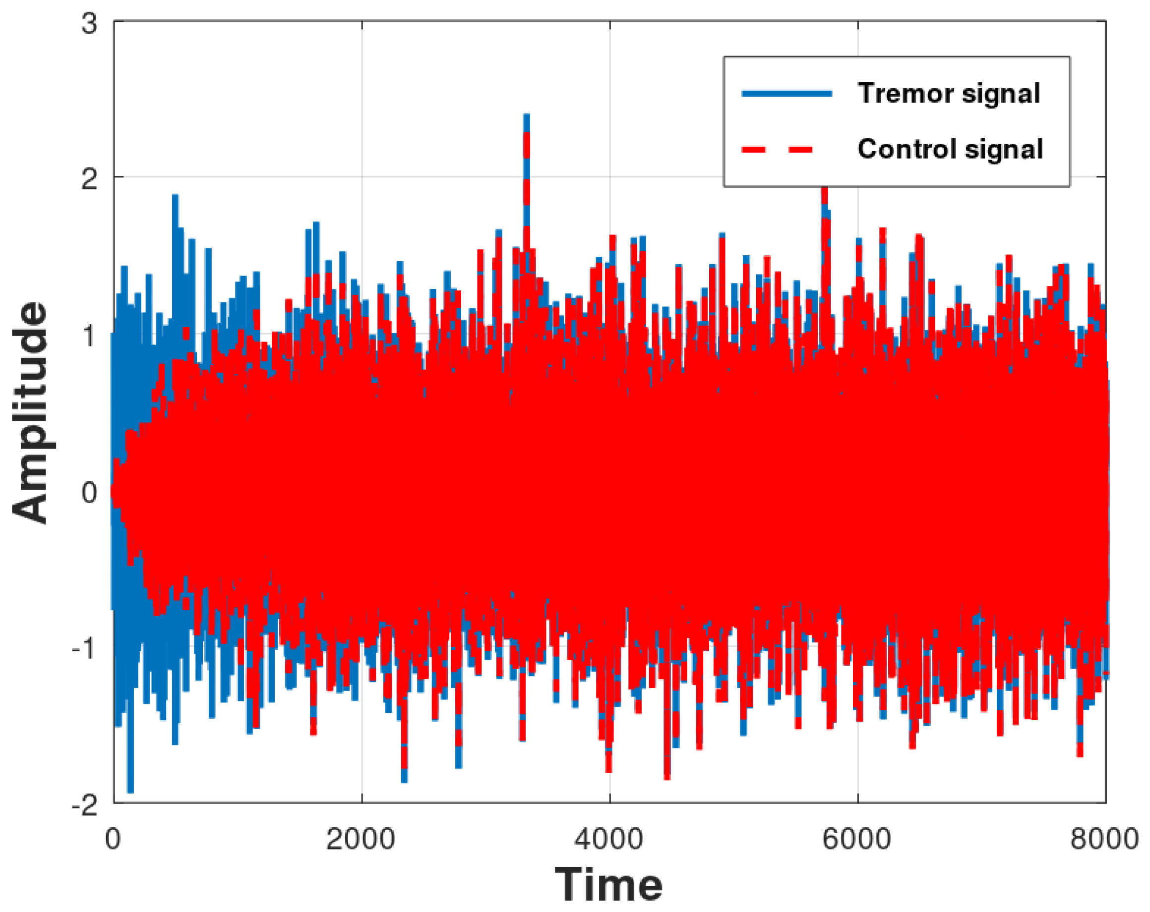
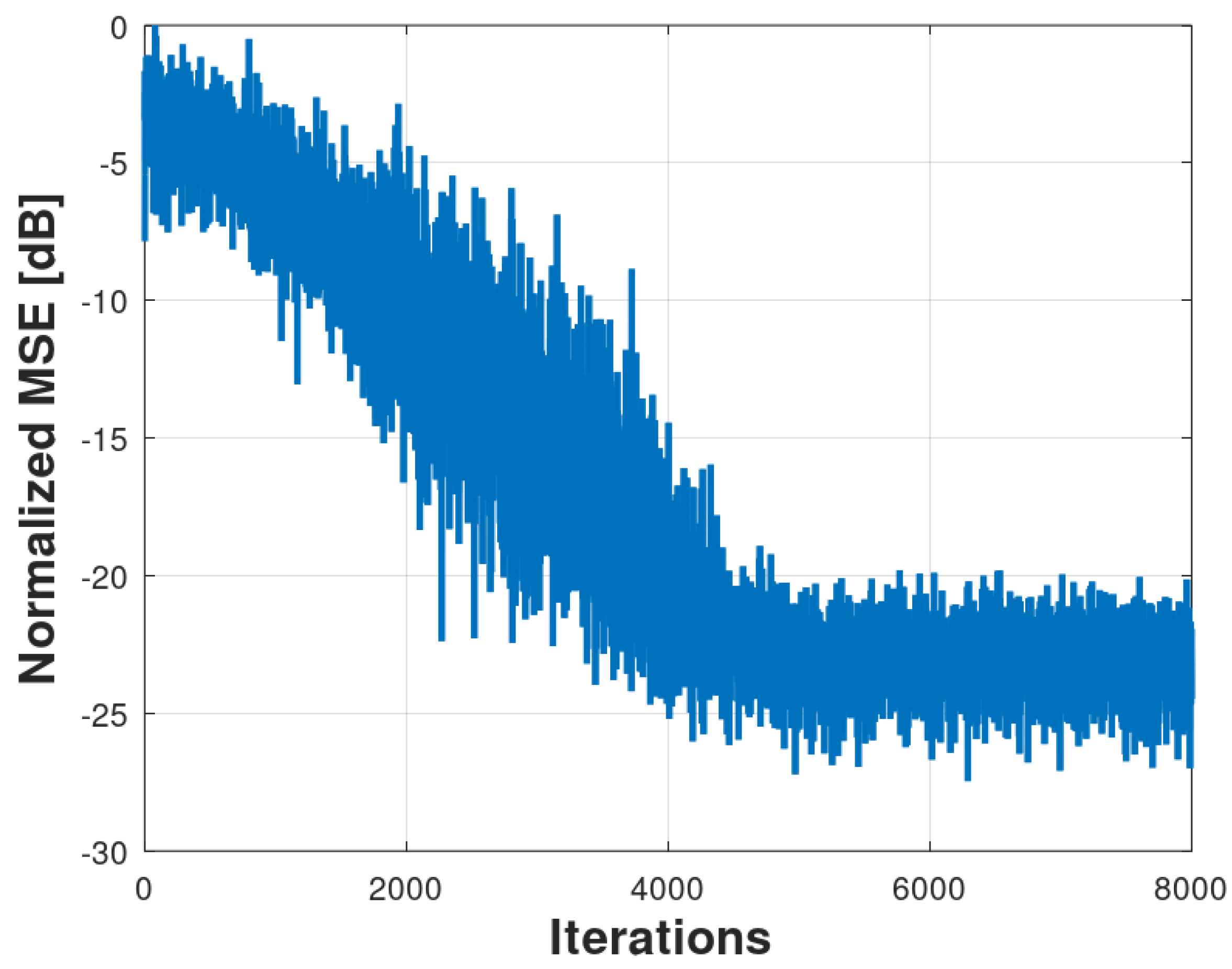
The behavior of the Fx-LMS algorithm (Scenario 1) in the active control of physiological tremor vibration is shown in
Figure 6. The steady state is reached after approximately 4000 samples.
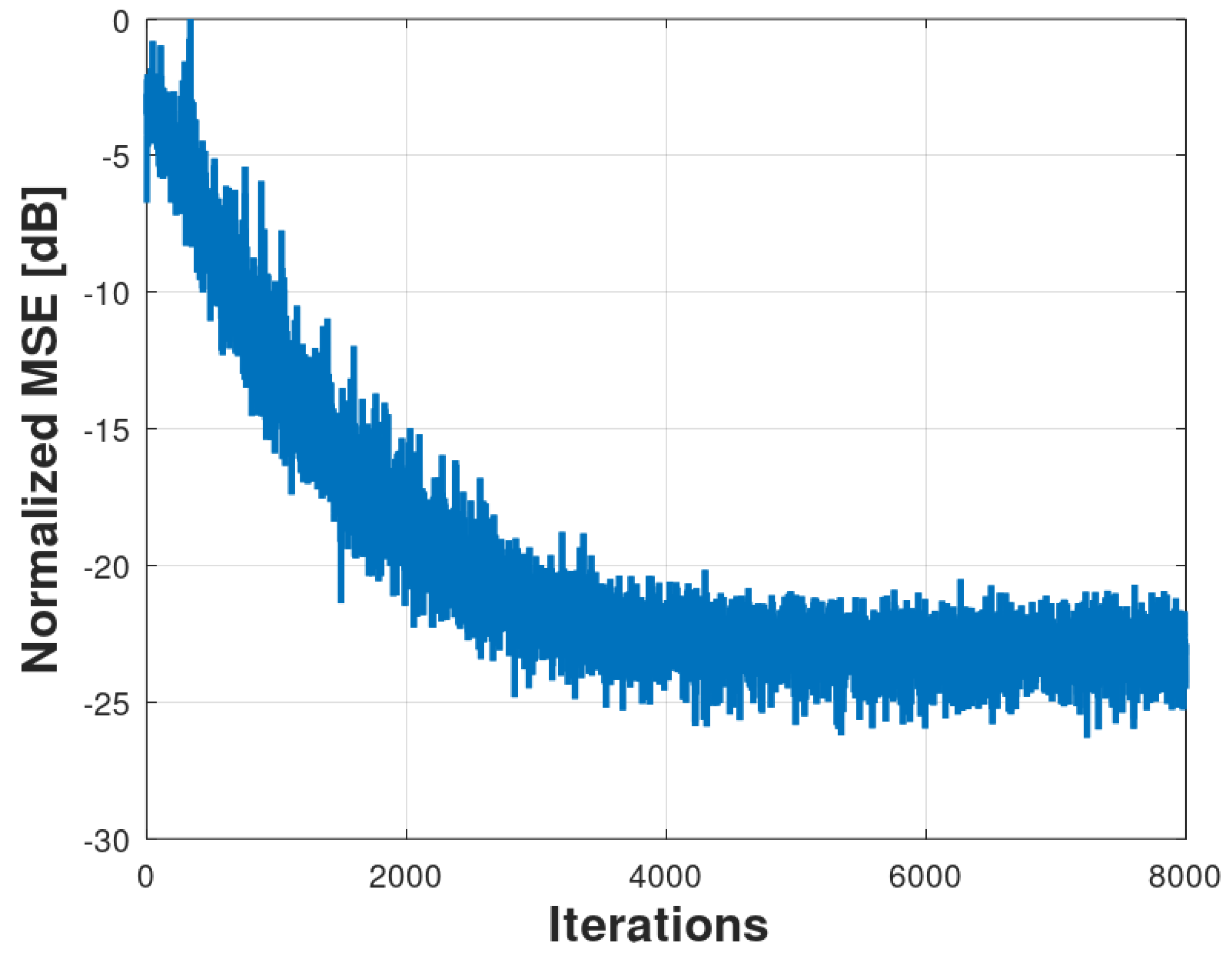
Figure 7 shows the result of the normalized mean square error (MSE) signal intensity, with a final mean value of -22 dB.
5.1.2. Scenario 2 (Fx-NLMS)
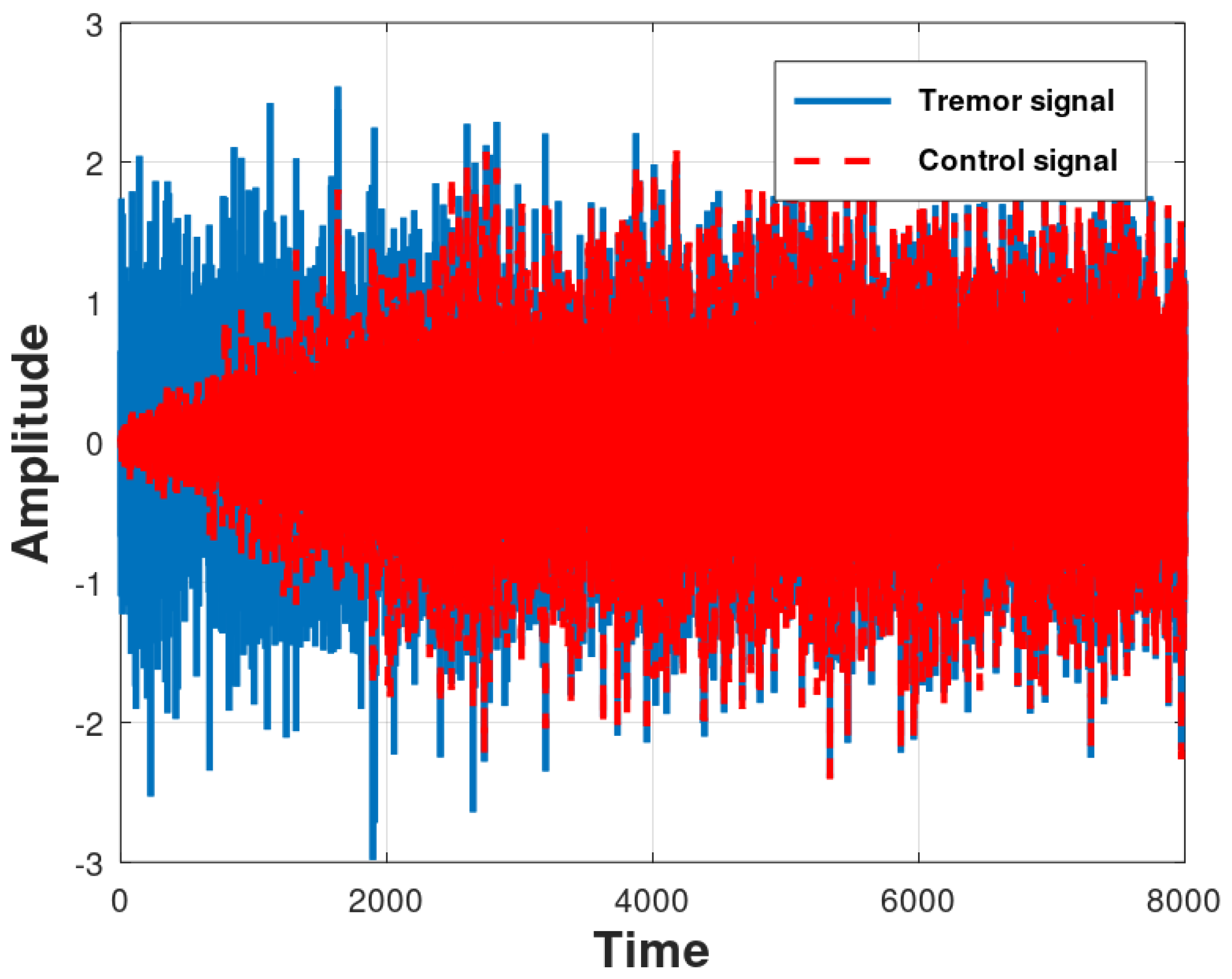
The Fx-NLMS algorithm has normalized data in both the main and secondary loops and its result for controlling the physiological tremor signal is illustrated by
Figure 8. In this case, approximately 4500 samples are needed for the control signal to converge, following the reference values, and it is enough to minimize the tremors.
Figure 9 shows the results for the normalized mean squared error signal data. As in scenario 1, the squared error, after convergence of the coefficients reaches an average value of -22 dB of attenuation.
5.1.3. Scenario 3 (Fx-LMS&NLMS)
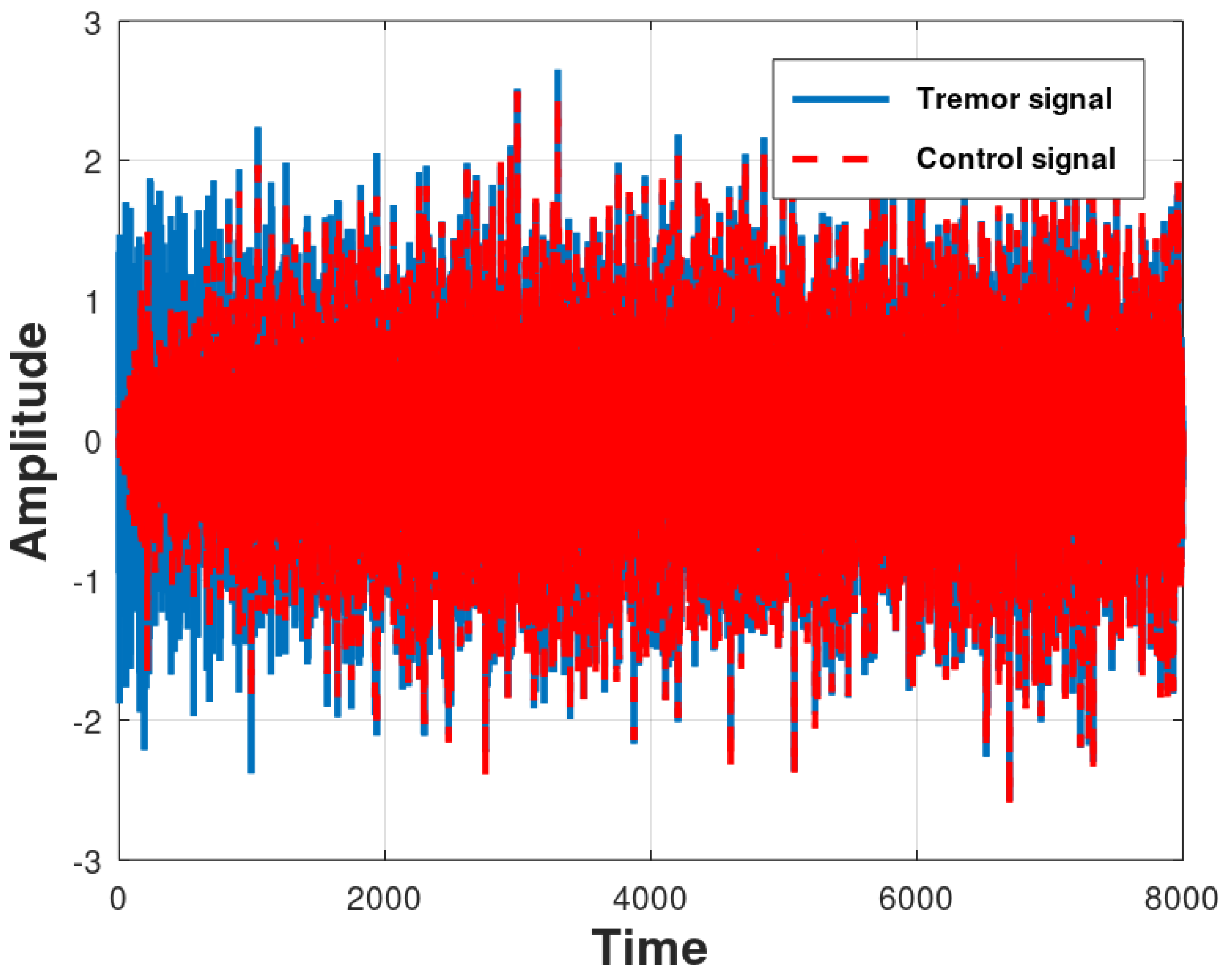
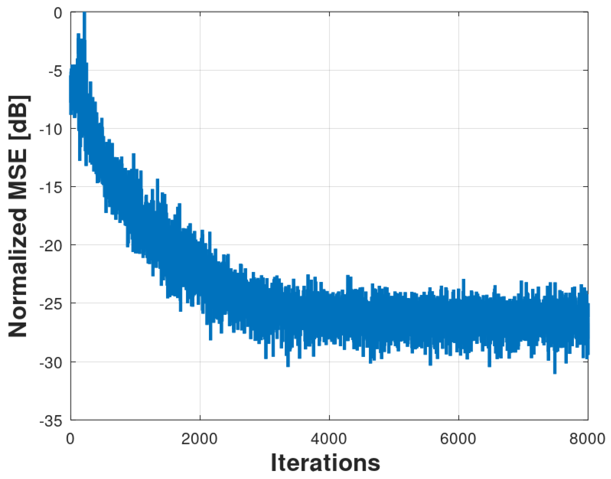
In scenario 3, hybrid, the control structure uses the Fx-LMS&NLMS algorithms, which have normalized data in the secondary loop error. This arrangement of algorithms is a suggestion of this work regarding a change in the normalization of the secondary path only. This combination enabled a gain in performance.
Figure 10 shows the control result of the algorithm, where the steady state is reached with approximately 4000 samples and reaches an average value of -28 dB of attenuation.
5.1.4. General comparison of Fx-LMS, Fx-NLMS, and Fx-NLMS&LMS
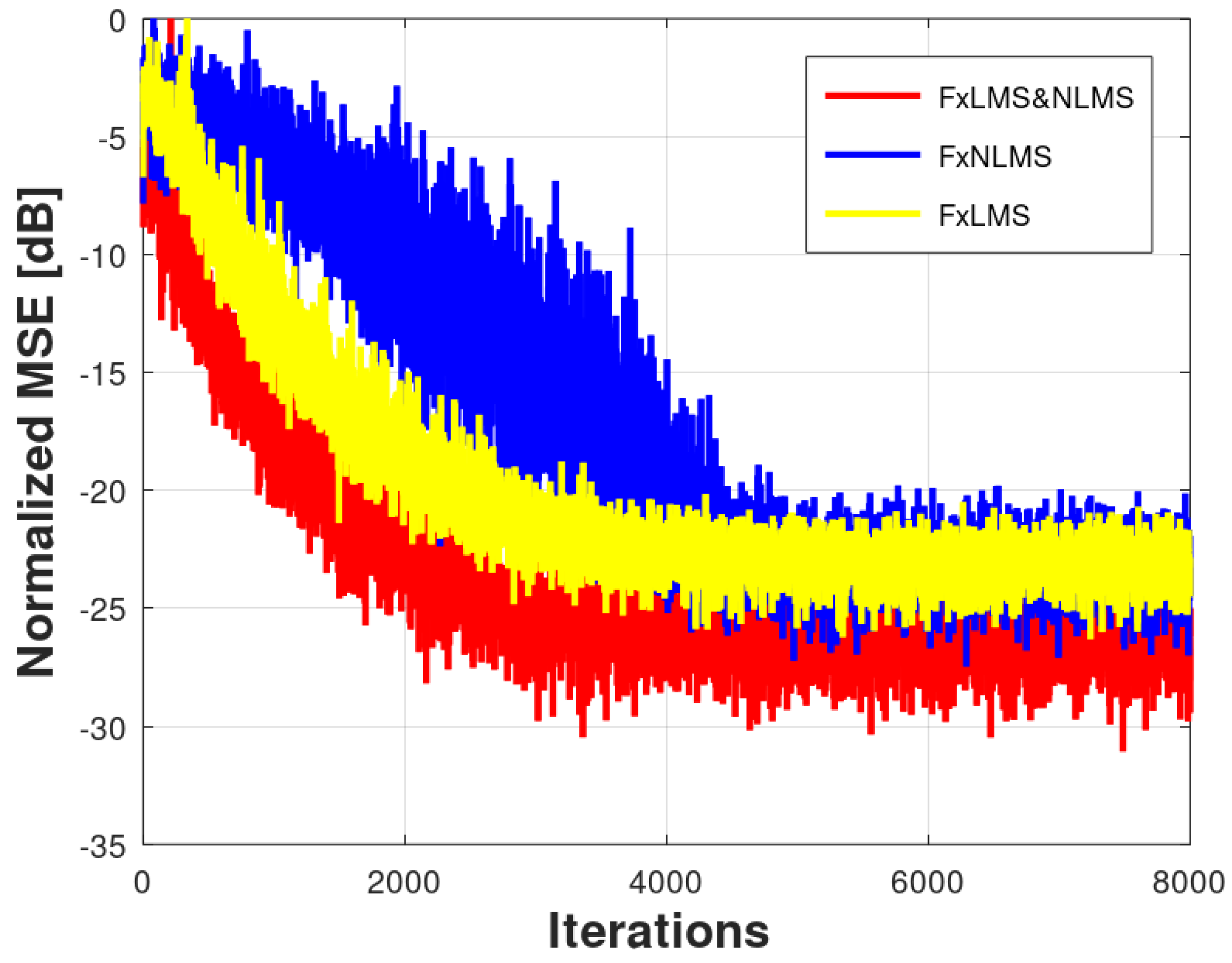
The Fx-LMS and Fx-NLMS algorithms, implemented in scenarios 1 and 2, respectively, presented a similar mean squared error attenuation level. The most relevant difference in behavior occurred in the convergence times of each one of them. The Fx-LMS algorithm reached an error of -22 dB in 4000 samples, 500 less than the time obtained in scenario 2.
The Fx-LMS&NLMS algorithm, implemented in scenario 3, proved to be faster if compared to NLMS algorithm, requiring 4000 samples to carry out the active control, a reduction of 30% compared to scenarios 1 and 2. This result can be attributed to fast response due to normalized filtering in the modeling of the only plant of
. This comparison can be seen in
Figure 12.
It is clear that an analysis in terms of computational complexity is necessary for a cost-benefit assessment. But, in a scenario where there is no complexity restriction, Fx-LMS&NLMS achieved faster convergence.
Table 2 presents more clearly the final comparison of the results in terms of the number of iterations and the amplitude and attenuation of the tremors in terms of square mean errors.
5.2. Simulation result of pathological tremors control
The dynamics of parkinsonian tremor are non-linear, deterministic, and chaotic [
32]. This is a totally different way of controlling what was previously shown with algorithms based on zero-mean and unitary variance Gaussian noise signals.
The control signal generated by the Fsinx-LMS algorithm will always try to follow the non-linearity and non-stationary nature of the tremor signal similar to that produced by the Parkinson tremor signal, as illustrated in
Figure 13. Analogous dynamics can be founded in [
33,
34]. Other solutions involving applied algorithms there are other scenarios with metrics and parameters can be viewed at [
35,
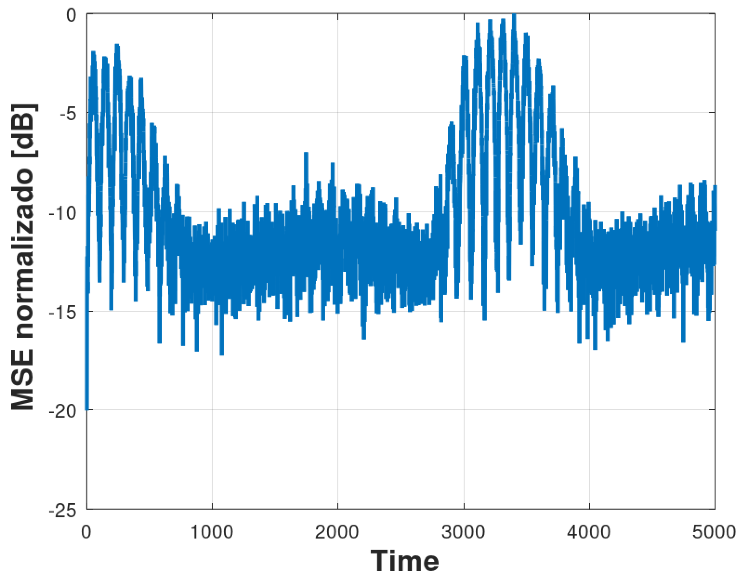
36]. In this way, the algorithm learns the dynamics of the tremor signal until its pattern changes and the algorithm needs to readapt itself, converging for the new coefficients. The MSE shown in
Figure 14 represents the operation of the adaptive algorithm. There is a high MSE initially, due to delay of the control system, until the error decreases drastically when the control signal follows the desired signal and the vibration pattern changes, and so the MSE increases again. This cycle repeats itself indefinitely. Unlike what happened in
Section 5.1, it is not possible to obtain a steady-state error since the MSE is always trying to adapt to the behavior of the system that changes with a periodic characteristic. But, it is possible to notice that the attenuation lies around 14 dB.
6. Conclusions
Adaptive algorithms usually have a complex nature, which demands a need for knowledge of statistics, mathematics, signal processing, and computing tools. This work sought to collaborate by presenting a discussion about these algorithms and a sequence of scientific tests that would allow their application in problems of Mechanical, Electronic, Computing, and Biomedical Engineering.
The bibliographic review allowed the construction and survey of the necessary concepts for the application of adaptive filtering techniques in order to actively control vibration. In addition, information about the problem to be solved and knowledge of the vibratory patterns are mentioned here. This search was based on mathematical models, avoiding the need for invasive data collection on patients.
From the obtained results it was noticed a great sensitivity to the model, the family of algorithms, and the parameters used. Active control of physiological and Parkinsonian tremors was presented using algorithms from the adaptive LMS family. The Fx-LMS&NLMS Algorithm showed the best response among the algorithms used in this research. Its difference from the others, Fx-LMS and Fx-NLMS, is only in the number of iterations. The algorithm that obtained the slowest response was the result of non-normalization in the primary mesh, where the plant of the system is initially recognized. The Fx-LMS algorithm is traditionally used in stroke, and can, in a way, serve as a parameter in relation to its variations, per hour used in the control of physiological tremors.
To provide active control of Parkinsonian tremors, the Fsinx-LMS algorithm was presented. Derived from Fx-LMS, this algorithm has only one additional block for the non-linearization of generated random signals, producing a random phase sinusoid. This was necessary so that the non-linearities of the model could be mapped by the adaptive system. It shows that there is a way to control deterministic and non-linear tremors, such as the tremor of Parkinson’s disease, through LMS-type algorithms, provided that the generated signals are non-linear.
This study can be extended to other types of algorithms, especially for Parkinsonian tremors. In this case, kernelized algorithms can produce better results in systems with non-linear characteristics present in models that replicate this type of pathology. These algorithms have been applied by the scientific community and produced good results. Other approaches for estimating nonlinear systems can yet be considered, such as [
33,
34,
37,
38,
39].
In addition, an implementation in embedded devices, DSP boards (Digital Signal Processor) can improve the understanding of the behavior of these algorithms in a practical scenario, which would later serve as a basis for the development of an electronic prototype with the embedded technology composed of a sensor and actuator to provide active control.
Notes
-
1Coefficients that characterize the behavior of the dynamic system.
-
2The internal model control systems are characterized by a control device composed by the controller and by a simulation of the process, the internal model.
-
3More details on this approach can be found in [17,31]
Author Contributions
Conceptualization, R.S.A., W.D.P., and R.C.B; methodology, R.S.A, and W.D.P.; analysis, R.S.A, J.C.T, W.D.P., and R.C.B; writing—original draft preparation, R.S.A, W.D.P, R.C.B, and J.C.T.; writing—review and editing, R.S.A, V.R.Q.L., W.D.P., J.F.d.P.S, and R.C.B All authors have read and agreed to the published version of the manuscript.
Institutional Review Board Statement
Not applicable.
Informed Consent Statement
Not applicable.
Data Availability Statement
Not applicable.
Acknowledgments
Fundação para a Ciência e a Tecnologia, I.P. (Portuguese Foundation for Science and Technology) by the project UIDB/05064/2020 (VALORIZA–Research Centre for Endogenous Resource 764 Valorization), and Project UIDB/04111/2020, ILIND–Instituto Lusófono de Investigação e Desenvolvimento, under project COFAC/ILIND/ COPELABS/3/2020.
Conflicts of Interest
The authors declare no conflict of interest.
Abbreviations
The following abbreviations are used in this manuscript:
| Active Vibration Control |
AVC |
| Analog-to-digital converters |
ADC |
| Digital Signal Processor |
DSP |
| Digital-to-analog converters |
DAC |
| Essential Tremors |
ET |
| Filtered-x Least Mean Square |
Fx-LMS |
| Filtered-x Normalized Least Mean Square |
Fx-NLMS |
| Finite Impulse Response |
FIR |
| Internal Model Control |
IMC |
| Least Mean Square |
LMS |
| Mean Square Error |
MSE |
| Normalized Least Mean Square |
NLMS |
| Parkinson’s Disease |
PD |
| Proportional, Integrative, and Derivative |
PID |
| Recursive Least Square |
RSL |
| World Health Organization |
WHO |
References
- Findley, L.J. Classification of tremors. Journal of Clinical Neurophysiology 1996, 13, 122–132. [Google Scholar] [CrossRef]
- Aryal, S.; Skinner, T.; Bridges, B.; Weber, J.T. The pathology of Parkinson’s disease and potential benefit of dietary polyphenols. Molecules 2020, 25, 4382. [Google Scholar] [CrossRef]
- Bhatia, K.P.; Bain, P.; Bajaj, N.; Elble, R.J.; Hallett, M.; Louis, E.D.; Raethjen, J.; Stamelou, M.; Testa, C.M.; Deuschl, G.; others. Consensus Statement on the classification of tremors. from the task force on tremor of the International Parkinson and Movement Disorder Society. Movement Disorders 2018, 33, 75–87. [Google Scholar] [CrossRef]
- Louis, E.D.; Ottman, R. Essential tremor. In Genetics of Movement Disorders; Elsevier, 2003; pp. 353–363. [CrossRef]
- Lenka, A.; Jankovic, J. Tremor syndromes: an updated review. Frontiers in Neurology 2021, 12. [Google Scholar] [CrossRef]
- Louis, E.D.; Ferreira, J.J. How common is the most common adult movement disorder? Update on the worldwide prevalence of essential tremor. Movement Disorders 2010, 25, 534–541. [Google Scholar] [CrossRef]
- Voon, V.; Napier, T.C.; Frank, M.J.; Sgambato-Faure, V.; Grace, A.A.; Rodriguez-Oroz, M.; Obeso, J.; Bezard, E.; Fernagut, P.O. Impulse control disorders and levodopa-induced dyskinesias in Parkinson’s disease: an update. The Lancet Neurology 2017, 16, 238–250. [Google Scholar] [CrossRef]
- Sweet, R.D.; McDowell, F. Five years’ treatment of Parkinson’s disease with levodopa: therapeutic results and survival of 100 patients. Annals of internal medicine 1975, 83, 456–463. [Google Scholar] [CrossRef]
- Lekshmi, A.; Ramachandran, K. Parkinson’s tremor suppression using active vibration control method. IOP Conference Series: Materials Science and Engineering. IOP Publishing, 2019, Vol. 577, p. 012056. [CrossRef]
- Kazi, S.; Mailah, M.; Zain, Z.M. Suppression of hand postural tremor via active force control method. Manufacturing Engineering, Automatic Control and Robotics, 2014. [Google Scholar]
- Turkistani, A. Development of an Effective Portable and Flexible Glove for Hand Tremor Suppression 2017. 2017. [Google Scholar]
- Chuanasa, J.; Songschon, S. Essential tremor suppression by a novel self-balancing device. Prosthetics and orthotics international 2015, 39, 219–225. [Google Scholar] [CrossRef]
- Hosseini, S.; Al-Jumaily, A.; Abboud, S.A. Active force control system for hand tremor suppression by different actuators. 2016 5th International Conference on Electronic Devices, Systems and Applications (ICEDSA). IEEE, 2016, pp. 1–4.
- Ibrahim, A.; Zhou, Y.; Jenkins, M.E.; Trejos, A.L.; Naish, M.D. Real-Time Voluntary Motion Prediction and Parkinson’s Tremor Reduction Using Deep Neural Networks. IEEE Transactions on Neural Systems and Rehabilitation Engineering 2021, 29, 1413–1423. [Google Scholar] [CrossRef]
- Kim, B.; Yoon, J.Y. Modified LMS strategies using internal model control for active noise and vibration control systems. Applied Sciences 2018, 8, 1007. [Google Scholar] [CrossRef]
- Jakubowski, J.; Kwiatos, K.; Chwaleba, A.; Osowski, S. Higher order statistics and neural network for tremor recognition. IEEE Transactions on Biomedical Engineering 2002, 49, 152–159. [Google Scholar] [CrossRef]
- Zhang, J.; Chu, F. Real-time modeling and prediction of physiological hand tremor. Proceedings.(ICASSP’05). IEEE International Conference on Acoustics, Speech, and Signal Processing, 2005. IEEE, 2005, Vol. 5, pp. v–645.
- Reeke, G.N.; Poznanski, R.R.; Lindsay, K.A.; Rosenberg, J.R.; Sporns, O. Modeling in the neurosciences: from biological systems to neuromimetic robotics; CRC Press, 2005.
- Dabis, H.; Moir, T. Least mean squares as a control system. International Journal of Control 1991, 54, 321–335. [Google Scholar] [CrossRef]
- Elliott, S.; Stothers, I.; Nelson, P. A multiple error LMS algorithm and its application to the active control of sound and vibration. IEEE Transactions on Acoustics, Speech, and Signal Processing 1987, 35, 1423–1434. [Google Scholar] [CrossRef]
- Song, P.; Zhao, H. Filtered-x least mean square/fourth (FXLMS/F) algorithm for active noise control. Mechanical Systems and Signal Processing 2019, 120, 69–82. [Google Scholar] [CrossRef]
- Martinek, R.; Rzidky, J.; Jaros, R.; Bilik, P.; Ladrova, M. Least mean squares and recursive least squares algorithms for total harmonic distortion reduction using shunt active power filter control. Energies 2019, 12, 1545. [Google Scholar] [CrossRef]
- Aslam, M.S.; Shi, P.; Lim, C.C. Robust Active Noise Control Design by Optimal Weighted Least Squares Approach. IEEE Transactions on Circuits and Systems I: Regular Papers, 2019. [Google Scholar]
- Widrow, B.; Glover, J.R.; McCool, J.M.; Kaunitz, J.; Williams, C.S.; Hearn, R.H.; Zeidler, J.R.; Dong, J.E.; Goodlin, R.C. Adaptive noise cancelling: Principles and applications. Proceedings of the IEEE 1975, 63, 1692–1716. [Google Scholar] [CrossRef]
- Widrow, B.; Stearns, S.D. Adaptive Signal Processing Prentice-Hall. Englewood Cliffs, NJ, 1985. [Google Scholar]
- Nascimento, V.H.; Silva, M.T. Adaptive filters. In Academic Press Library in Signal Processing; Elsevier, 2014; Vol. 1, pp. 619–761.
- Paulo, S.D. Adaptive filtering: algorithms and practical implementation; Springer US, 2013.
- Poularikas, A.D. Adaptive filtering: Fundamentals of least mean squares with MATLAB®; CRC Press, 2017.
- Sayed, A.H. Fundamentals of adaptive filtering; John Wiley & Sons, 2003.
- Ardekani, I.T.; Abdulla, W.H. Theoretical convergence analysis of FxLMS algorithm. Signal Processing 2010, 90, 3046–3055. [Google Scholar] [CrossRef]
- Brockwell, P.; Dahlhaus, R. Generalized Levinson–Durbin and burg algorithms. Journal of Econometrics 2004, 118, 129–149. [Google Scholar] [CrossRef]
- Beuter, A.; Glass, L.; Mackey, M.C.; Titcombe, M.S. Nonlinear dynamics in physiology and medicine; 2003.
- Parreira, W.D.; Costa, M.H.; Bermudez, J.C. Stochastic behavior analysis of the Gaussian KLMS algorithm for a correlated input signal. Signal Processing 2018, 152, 286–291. [Google Scholar] [CrossRef]
- Dos Santos, V.A.; Parreira, W.D.; Fernandes, A.M.D.R.; Ovejero, R.G.; Leithardt, V.R.Q. Improving Speaker Recognition in Environmental Noise with Adaptive Filter. IEEE Access 2022. [Google Scholar] [CrossRef]
- Leite, M.; Parreira, W.D.; Fernandes, A.M.d.R.; Leithardt, V.R.Q. Image Segmentation for Human Skin Detection. Applied Sciences 2022, 12. [Google Scholar] [CrossRef]
- de Freitas, M.P.; Piai, V.A.; Farias, R.H.; Fernandes, A.M.R.; de Moraes Rossetto, A.G.; Leithardt, V.R.Q. Artificial Intelligence of Things Applied to Assistive Technology: A Systematic Literature Review. Sensors 2022, 22. [Google Scholar] [CrossRef] [PubMed]
- Parreira, W.D.; Bermudez, J.C.M.; Richard, C.; Tourneret, J.Y. Stochastic behavior analysis of the Gaussian kernel least-mean-square algorithm. IEEE Transactions on Signal Processing 2012, 60, 2208–2222. [Google Scholar] [CrossRef]
- dos SP Soares, A.; Parreira, W.D.; Souza, E.G.; de Almeida, S.J.; Diniz, C.M.; Nascimento, C.D.; Stigger, M.F. Energy-based voice activity detection algorithm using Gaussian and Cauchy kernels. 2018 IEEE 9th Latin American Symposium on Circuits & Systems (LASCAS). IEEE, 2018, pp. 1–4.
- Soares, A.d.S.P.; Parreira, W.D.; Souza, E.G.; Nascimento, C.d.D.d.; Almeida, S.J.M.d. Voice Activity Detection Using Generalized Exponential Kernels for Time and Frequency Domains. IEEE Transactions on Circuits and Systems I: Regular Papers 2019, 66, 2116–2123. [Google Scholar] [CrossRef]
|
Disclaimer/Publisher’s Note: The statements, opinions and data contained in all publications are solely those of the individual author(s) and contributor(s) and not of MDPI and/or the editor(s). MDPI and/or the editor(s) disclaim responsibility for any injury to people or property resulting from any ideas, methods, instructions or products referred to in the content. |
© 2023 by the authors. Licensee MDPI, Basel, Switzerland. This article is an open access article distributed under the terms and conditions of the Creative Commons Attribution (CC BY) license (http://creativecommons.org/licenses/by/4.0/).
