Necessity to Use the True Gravity in Large Scale Atmospheric Modeling

Preprint

Article

Necessity to Use the True Gravity in Large Scale Atmospheric Modeling

Altmetrics

Downloads

153

Views

Comments

Peter C. Chu^*

This version is not peer-reviewed

Submitted:

04 February 2023

Posted:

07 February 2023

You are already at the latest version

Alerts

Abstract

Newton’s law of universal gravitation applies between two point-masses. True gravitation of solid Earth is volume integration of gravitation of all point-masses inside the solid Earth on a point-mass in atmosphere. However, in meteorology the Earth “shrinks” into a point-mass located at Earth center with entire Earth mass to identify the Earth gravitation (untrue). Combination of untrue gravitational and centrifugal accelerations gives effective gravity (geff). Combination of true gravitational and centrifugal accelerations leads to true gravity (g). The true gravity g minus the effective gravity geff is the gravity disturbance vector, δg = g – geff. With the true gravity g used in the basic equations, seven non-dimensional numbers are proposed to identify the importance of δg versus traditional forcing terms such as horizontal pressure gradient force and Coriolis force. These non-dimensional numbers are calculated from two publicly available datasets with the geoid undulation (N) from the static gravity field model EIGEN-6C4 and long-term mean geopotential height (Z), wind velocity (u, v), and temperature (Ta) at 12 pressure levels in troposphere from the NCEP/NCAR reanalyzed climatology. The results demonstrate δg nonnegligible in hydrostatic equilibrium, geostrophic wind, geostrophic vorticity, Ekman pumping, Q vector, and Omega equation, but negligible in thermal wind relation.

Keywords:

Subject: Environmental and Earth Sciences - Atmospheric Science and Meteorology

1. Introduction

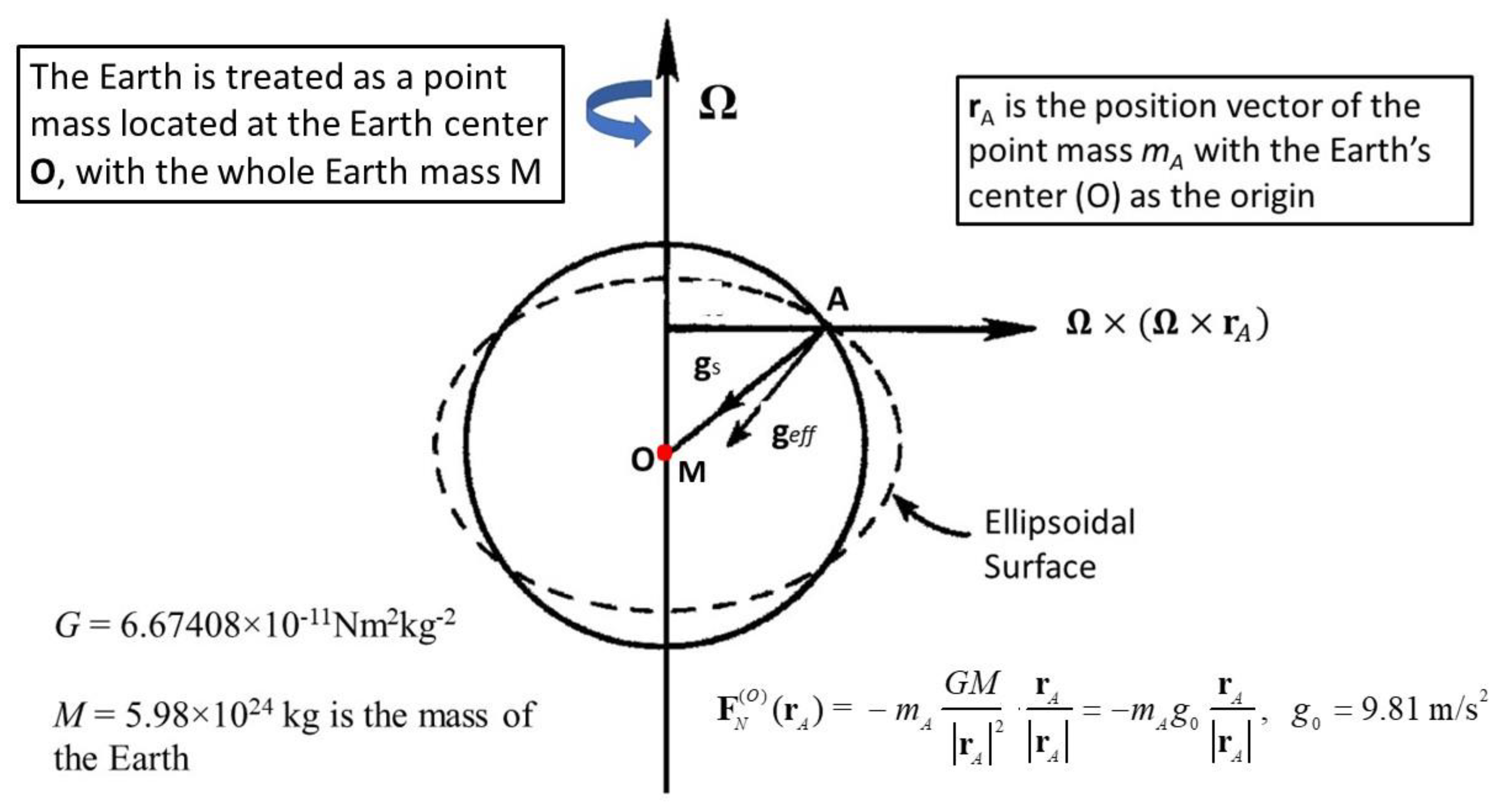
Every meteorologist including the author from very beginning of her/his career learned that the Earth gravity on a point-mass in atmosphere (m_A) at location r_A consists of Earth gravitation and centrifugal force with the Earth center (O) as the origin of the position vector r_A (Figure 1). The solid Earth “shrinks” into a point-mass located at the Earth center with the entire Earth mass to get the Earth gravitation. With such a treatment, the Earth gravitation on m_A, given by F

\binom{(O)}{N}

(r_A), is between the Earth point-mass M_O (at point O) and atmospheric point-mass m_A,

F_{N}^{(O)} (r_{A}) = - m_{A} \frac{G M}{{| r_{A} |}^{2}} \frac{r_{A}}{| r_{A} |} = - m_{A} g_{0} \frac{r_{A}}{| r_{A} |}, g_{0} = 9.81 {m / s}^{2}

(1)

where G = 6.67408×10^-11Nm²kg^-2, is the Newtonian gravitational constant; and M = 5.98×10²⁴ kg is the mass of the Earth. Since F

\binom{(O)}{N}

(r_A) in Eq.(1) is calculated through shrinking the solid Earth into a point-mass M_O. It is not true and therefore should be called the untrue Earth gravitation.

Let Ω be the Earth’s angular velocity with |Ω| = 2π/(86164 s). Combining the untrue gravitation (F

\binom{(O)}{N})

with the centrifugal force (F_C) on the point-mass m_A

F^{(O)} (r_{A}) = F_{N}^{(O)} (r_{A}) + F_{C} (r_{A}) = - m_{A} g_{0} \frac{r_{A}}{| r_{A} |} + m_{A} Ω \times (Ω \times r_{A})

(2)

leads to the effective gravity (g_eff, sometimes called normal gravity, or apparent gravity) [1] (pp 12-14)

g_{e f f} = - g_{0} \frac{r_{A}}{| r_{A} |} + Ω \times (Ω \times r_{A})

(3)

The effective gravity g_eff is non-radial (not in the direction of r_A) but changes little with latitude or height. The rotation causes equatorial bulge and polar flattening, i.e., uniform ellipsoidal Earth. Let k be the unit vector perpendicular to the ellipsoidal Earth surface. The effective gravity g_eff at the Earth surface is given by (https://glossary.ametsoc.org/wiki/Gravity)

g_{e f f} = - g (φ) k, g (φ) = 9 . 806160 (1 - 0.0026373 \cos 2 φ + 0.0000059 \cos^{2} 2 φ)

(4)

where φ is the latitude.

To solve the non-radial nature of g_eff, orthogonal curvilinear coordinate systems, i.e., the geopotential coordinates (more accurately called the effective geopotential coordinates) have been used. Among them, the oblate spheroid coordinate system (λ, φ, z) with (i, j, k) the corresponding unit vectors is optimal since it describes the ellipsoidal shape more accurately. However, the error is less than 0.17% between polar spherical coordinate and oblate spherical coordinate systems [2] (P.92). The geophysically realistic, ellipsoidal, analytically tractable (GREAT) coordinates was presented [3] to make that the horizontal coordinate surfaces coincide with the effective geopotential (Φ_eff) surfaces and to ensure that there is no component of effective gravity (g_eff) in any direction tangential to coordinate surfaces (i.e., no horizontal compoenent in g_eff),

g_{e f f} = - \frac{d Φ_{e f f}}{d z} k

(5a)

where the direction of k is defined as the vertical in meteorology. The effective geopotential Φ_eff is given by [2] (P.46, Equation 3.5.2) [5,6]

g (φ) = \frac{d Φ_{e f f}}{d z} \approx g_{0}, Φ_{e f f} \approx g_{0} z

(5b)

where z is the height of the point mass in atmosphere with z = 0 at the Earth ellipsoidal surface. Vertical integration of (5b) from z = 0 to the height of the point mass in atmosphere (z) leads to

Z = \frac{1}{g_{0}} \int_{0}^{z} \frac{d Φ_{e f f}}{d z} d z'

(6)

where Z is the effective geopotential height of the point mass. The two heights (z and Z) are numerically interchangeable for most meteorological purpose (see website: https://glossary.ametsoc.org/wiki/Geopotential_height). The effective gravity g_eff with no horizontal component has been used in atmospheric dynamics and modeling as if it were the true gravity.

A question arises: Is it reasonable to shrink the solid Earth into a point-mass with the entir Earth mass (M) concentrated at the Earth center (O) in calculating the Earth gravitation? The answer is NO because the solid Earth contains infinite number of point-masses. The Newton’s law of universal gravitation in today’s language states that every point-mass attracts every other point mass by a force acting along the line intersecting the two points. The force is proportional to the product of the two point-masses, and inversely proportional to the square of the distance between them (see website https://en.wikipedia.org/wiki/Newton%27s_law_of_universal_gravitation.)

Let r be the position vector of a point inside the solid Earth, σ(r) be the mass density, and dΠ be the infinitesimally small volume (around r). The point-mass at r is represented by

d m (r) = σ (r) d Π .

The Newton’s gravitation of point-mass dm(r) on a point mass m_A at location r_A in atmosphere is given by

d F_{N} (r_{A}) = G m_{A} d m (r) \frac{(r - r_{A})}{{| r - r_{A} |}^{3}} = G m_{A} σ (r) \frac{(r - r_{A})}{{| r - r_{A} |}^{3}} d Π

(7a)

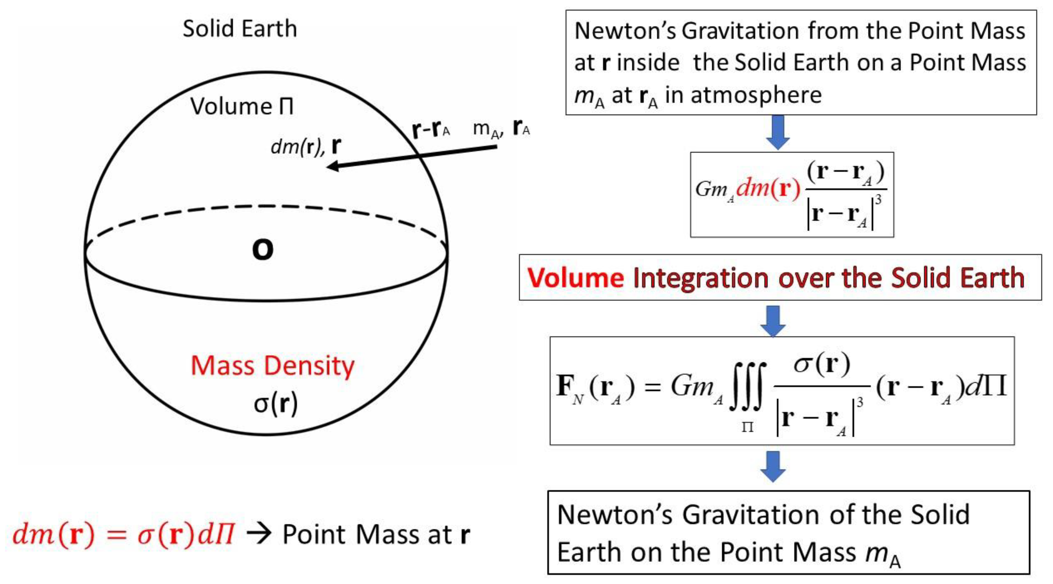
The gravitation of the whole Earth on the point-mass m_A is the volume integration (Figure 2) [4] (P.72, Equation 6.4),

F_{N} (r_{A}) = \underset{Π}{∭} d F_{N} (r_{A}) = G m_{A} \underset{Π}{∭} σ (r) \frac{(r - r_{A})}{{| r - r_{A} |}^{3}} d Π

(7b)

where Π is the Earth volume. Let σ₀ be the averaged mass density of the solid Earth. Then Eq.(7b) becomes

F_{N} (r_{A}) = - m_{A} \frac{G M}{{| r_{A} |}^{3}} r_{A} + G m_{A} \underset{Π}{∭} \frac{[σ (r) - σ_{0}]}{{| r - r_{A} |}^{3}} (r - r_{A}) d Π

(8)

Combine the true gravitational force (F_N) and the centrifugal force (F_C) on the point mass A in atmosphere

F (r_{A}) = F_{N} (r_{A}) + F_{C} (r_{A}) = - m_{A} g_{0} \frac{r_{A}}{| r_{A} |} + m_{A} Ω \times (Ω \times r_{A}) + G m_{A} \underset{Π}{∭} \frac{[σ (r) - σ_{0}]}{{| r - r_{A} |}^{3}} (r - r_{A}) d Π

(9)

Correspondingly the true Earth gravity on the point mass m_A in atmosphere [using Eqs.(2) and (9)] is given by

g = g_{e f f} + δ g, δ g \equiv \frac{1}{m_{A}} [F_{N} (r_{A}) - F_{N}^{(O)} (r_{A})] = G \underset{Π}{∭} \frac{[σ (r) - σ_{0}]}{{| r - r_{A} |}^{3}} (r - r_{A}) d Π

(10)

Here, g is the true gravity; δg, with evident horizontal components, is the true gravitational acceleration minus untrue gravitational acceleration, and called the gravity disturbance vector. δg is a major variable and quantified by gravity field models along with observations in geodesy and solid Earth dynamics, however, it is totally neglected in atmospheric dynamics and modeling.

The gravity disturbance vector δg was recently found important in ocean dynamics especially in Ekman transport [7]. However, importance of δg in large-scale atmospheric dynamics has not been recognized. The objective of this study is to show the importance of δg in atmospheric dynamics.

2. Materials and Methods

2.1. True Geopotential

The gravity disturbance vector δg due to the nonuniform mass density σ(r) inside the Earth [i.e., σ(r) ≠ σ₀, see Eq.(10)] is represented by the disturbing gravity potential T (δg ≡

\nabla

₃T) with

\nabla

₃ the three dimensional vector differential operator. The true geopotential (Φ) is given by [8]

Φ = Φ_{e f f} - T (λ, φ, z)

(11)

Due to independence of δg on the Earth rotation [see Eq.(10)], the disturbing gravity potential T outside the Earth masses can be expanded in the polar spherical coordinates [9]

T (λ, φ, z) = \frac{G M}{(R + z)} {\sum_{l = 2}^{l_{\max}} \sum_{m = 0}^{l} (\frac{R}{R + z})}^{l} [(C_{l, m} - C_{l, m}^{e l}) \cos m λ + S_{l, m} \sin m λ] P_{l, m} (\sin φ)

(12)

where R = 6.3781364×10⁶ m is the Earth radius; (C_l,m,

C \binom{e l}{l, m},

S_l,m) are the harmonic geopotential coefficients with

C \binom{e l}{l, m}

belonging to the reference ellipsoid; P_l,m(sinφ) are the Legendre associated functions with (l, m) the degree and order of the harmonic expansion; and l_max is the order of the gravity field model. The larger the value of l_max, the higher the resolution of the disturbing gravity potential T.

Usually, a static gravity field model in geodetic community provides the data for disturbing gravity potential T at z = 0,

\begin{array}{l} T (λ, φ, 0) = \frac{G M}{R} \sum_{l = 2}^{l_{\max}} \sum_{m = 0}^{l} [(C_{l, m} - C_{l, m}^{e l}) \cos m λ + S_{l, m} \sin m λ] P_{l, m} (\sin φ), \\ T_{z} (λ, φ, 0) = \frac{\partial T (λ, φ, 0)}{\partial z} \end{array}

(13)

where T_z (vertical component of the gravity disturbance vector δg) is called the gravity disturbance in geodesy. According to (12), the ratio between T(λ, φ, z) and T(λ, φ, 0) through the troposphere can be roughly estimated by

| \frac{T (λ, φ, z)}{T (λ, φ, 0)} | \approx \frac{R}{(R + z)}, H \geq z \geq 0

(14)

where H is the height of the troposphere. Because the Earth radius (R) is more than 3 orders of magnitude larger than H, the disturbing gravity potential at the surface (z =0), T(λ, φ, 0), and its z-derivative T_z(λ, φ, 0) are used approximately for the whole troposphere in this study,

T (λ, φ, z) \approx T (λ, φ, 0), T_{z} (λ, φ, z) \approx T_{z} (λ, φ, 0), H \geq z \geq 0

(15)

Besides, the surface disturbing gravity potential T(λ, φ, 0) is related to the geoid height (N) by the Bruns’ formula [10]

T (λ, φ, 0) = g_{0} N (λ, φ)

(16)

where N is the geoid undulation. Substitution of (15) into (11) leads to the true geopotential in the troposphere approximately given by

Φ = Φ_{e f f} - T \approx Φ_{e f f} - g_{0} N (λ, φ)

(17)

2.2. Data Sources

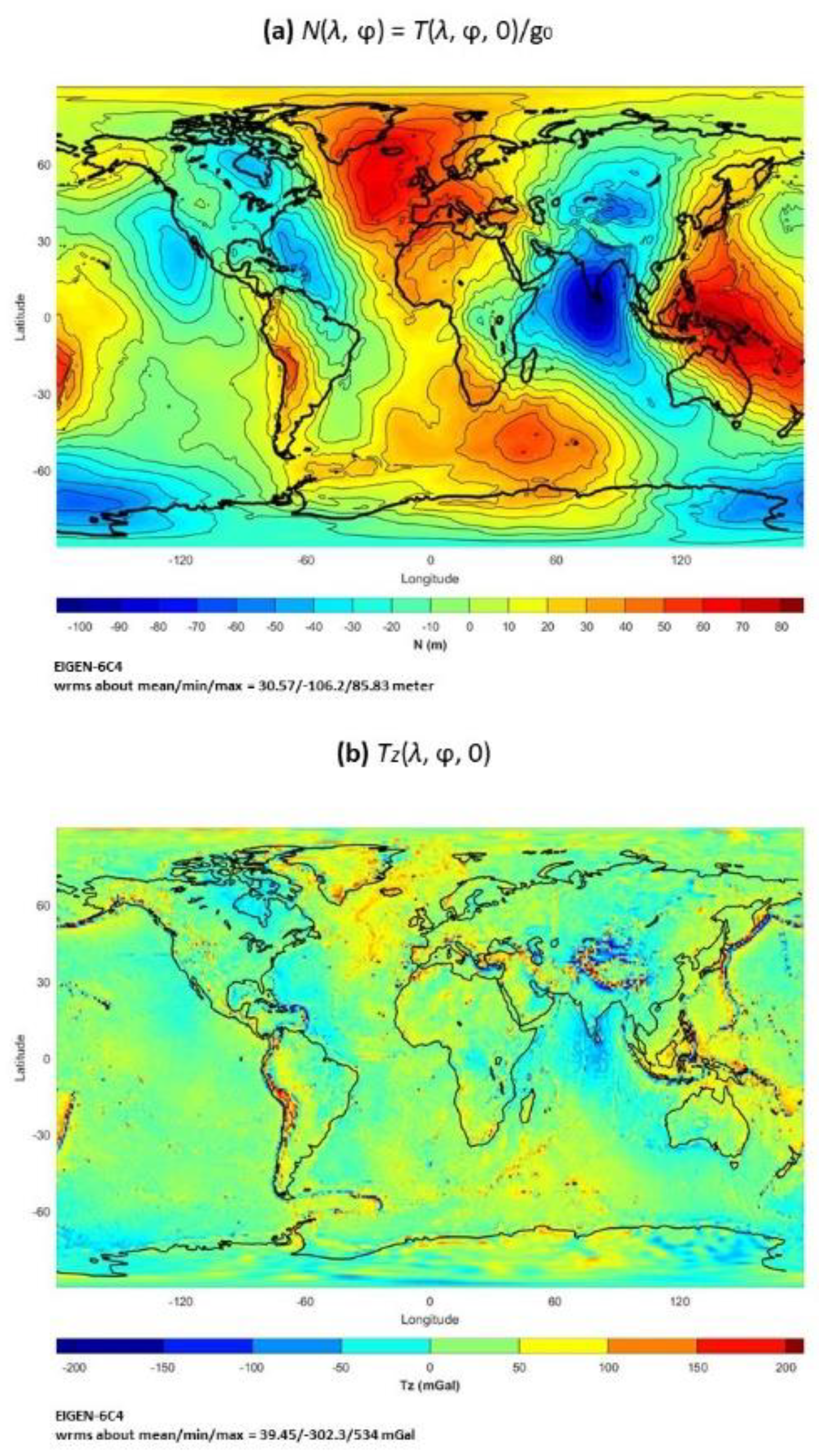
Two independent and publicly available datasets are used in this study: (a) ICGEM global static gravity field model EIGEN-6C4 (http://icgem.gfz-potsdam.de/home) [9] for [N(λ, φ), T_z(λ, φ, 0)], and (b) NCEP/NCAR reanalyzed monthly long-term mean (effective) geopotential height (Z), wind velocity (u, v), and temperature (T_a) at 12 pressure levels 1,000, 925, 850, 700, 600, 500, 400, 300, 250, 200, 150, and 100 hPa (https://psl.noaa.gov/data/gridded/data.ncep.reanalysis.derived.pressue.html), are used to identify the importance of the gravity disturbance vector δg on atmospheric dynamics. The long-term annual mean (Z, u, v, T_a) are calculated from the long-term monthly mean data before the identification. The horizontal variability of N shows a range from a minimum of -106.2 m to a maximum of 85.83 m with a mean of 30.57 m (Figure 3a), which is comparable to the horizontal variability of Z at 1,000 hPa (-140 m to 240 m) (Figure 4a). The horizontal variability of T_z shows a range from a minimum of -302.3 mGal to a maximum of 534 mGal with a mean of 39.45 mGal (1 mGal = 10^-5 m s^-2) (Figure 3b).

Note that the EIGEN-6C4 [N(λ, φ), T_z(λ, φ, 0)] data are represented in the polar spherical coordinate system since the gravity disturbance vector δg is independent on the Earth rotation [see Eq.(10)]. However, the NCEP/NCAR reanalyzed (Z, u, v, T_a) data are represented in the effective geopotential coordinate system (i.e., the oblate spheroidal coordinates) with the pressure as the vertical coordinate. The difference between the polar spherical and oblate spheroidal coordinate systems are estimated less than 0.17% [2] (P92), and likely to be small except perhaps in long-term simulations in which small systematic differences may accumulate [11,12]. In this study, all the computation is in the polar spherical coordinates including the NCEP/NCAR reanalyzed data. The effect of the gravity disturbance vector (δg) on atmospheric dynamics is negligible if the ratio of forcing terms due to the gravity disturbance vector over due to the others (such as the horizontal pressure gradient, and Coriolis force) is comparable to or not substantially larger than the error of using the polar spherical coordinates for the meteorological datasets (i.e., 0.17%) [2] (P92).

2.3. Horizontal Gradients of T in Pressure as Vertical Coordinate

Consider the local effective geopotential coordinate system with z as the vertical coordinate (i.e., the direction of k) and (x, y) the horizontal coordinates. A derivative with respect to x between the z and p as the vertical coordinates is given by

{(\frac{\partial}{\partial x})}_{p} = {(\frac{\partial}{\partial x})}_{z} + {(\frac{\partial z}{\partial x})}_{p} \frac{\partial}{\partial z}

(18)

Using (18) to the derivative of p gives

0 = {(\frac{\partial p}{\partial x})}_{z} + {(\frac{\partial z}{\partial x})}_{p} \frac{\partial p}{\partial z},

(19)

and to the derivative of T gives

{(\frac{\partial T}{\partial x})}_{p} = {(\frac{\partial T}{\partial x})}_{z} + {(\frac{\partial z}{\partial x})}_{p} \frac{\partial T}{\partial z}

(20)

Here, the hydrostatic balance is represented by

\frac{\partial p}{\partial z} = - ρ g_{0}, Φ_{e f f} = g_{0} z

(21)

Elimination of

{(\partial z / \partial x)}_{p}

from (19) and (20) and use of (21) give

{(\frac{\partial T}{\partial x})}_{z} = {(\frac{\partial T}{\partial x})}_{p} - {(\frac{\partial Φ_{e f f}}{\partial x})}_{p} (\frac{1}{g_{0}} \frac{\partial T}{\partial z})

(22)

With the same procedure for the derivative of T with respect to y, we have

\nabla_{z} T = \nabla T - (T_{z} / g_{0}) \nabla Φ_{e f f}

(23)

where

\nabla

(or

\nabla

_z) is the horizontal vector differential operator in p (or z) as the vertical coordinate. Figure 3b shows that T_z varies between -302.3 mGal and 534.0 mGal, which leads to

| T_{z} / g_{0} | < 534 mGal / (9 {. 81 m s}^{- 2}) = 5 . 443 \times 10^{- 4}

(24)

3. Results

3.1. Equation of Motion with the True Geopotential

With the true geopotential (Φ), the horizontal component of the dynamic equation in the pressure as the vertical coordinate is given by

\frac{D U}{D t} + f k \times U = - \nabla Φ + F

(25)

where f is the Coriolis parameter; U = (u, v), is the horizontal velocity vector; F is the frictional force; and

\frac{D}{D t} = \frac{\partial}{\partial t} + U • \nabla + ω \frac{\partial}{\partial p}, ω = \frac{d p}{d t}

(26)

Here, ɷ is the vertical velocity in the pressure as the vertical coordinate. Substitution of (11) into (25) leads to

\frac{D U}{D t} + f k \times U = - \nabla Φ_{e f f} + \nabla T + F, Φ_{e f f} = g_{0} Z

(27)

Substitution of (23) into (27) lead to

\frac{D U}{D t} + f k \times U = - [1 - (T_{z} / g_{0})] \nabla Φ_{e f f} + \nabla_{z} T + F)

which gives

\frac{D U}{D t} + f k \times U = - \nabla Φ_{e f f} + \nabla_{z} T + F

(28)

Here, the inequality (24) is used. Eq.(28) shows that the horizontal gradient

\nabla T

(or

\nabla N)

in p as the vertical coordinate can be replaced by

\nabla

_zT (or

\nabla

_zN) in z as the vertical coordinate,

T = g_{0} N, \nabla T \equiv horizontal component of δ g \approx \nabla_{z} T, \nabla^{2} T \approx \nabla_{z}^{2} T

(29)

Non-dimensional B and C numbers are defined by

B \equiv \frac{O (| \nabla T |)}{O (| \nabla Φ_{e f f} |)} \approx \frac{g_{0} O (| \nabla_{z} N |)}{O (| \nabla Φ_{e f f} |)} = \frac{O (| \nabla_{z} N |)}{O [| \nabla Z |]}, C \equiv \frac{O (| \nabla T |)}{O (| f U |)} \approx \frac{g_{0} O (| \nabla_{z} N |)}{O (| f U |)}

(30)

to identify the importance of the gravity disturbance vector (δg) versus the effective gravity (g_eff) (B number) and the Coriolis force (C number). Here (15), (16), and (29) are used. Hereafter the global mean is taken to represent the order of magnitude. Eq. (30) becomes

B = \frac{mean (| \nabla_{z} N |)}{mean [| \nabla Z |]}, C = g_{0} \frac{mean (| \nabla_{z} N |)}{mean (| f U |)}

(31)

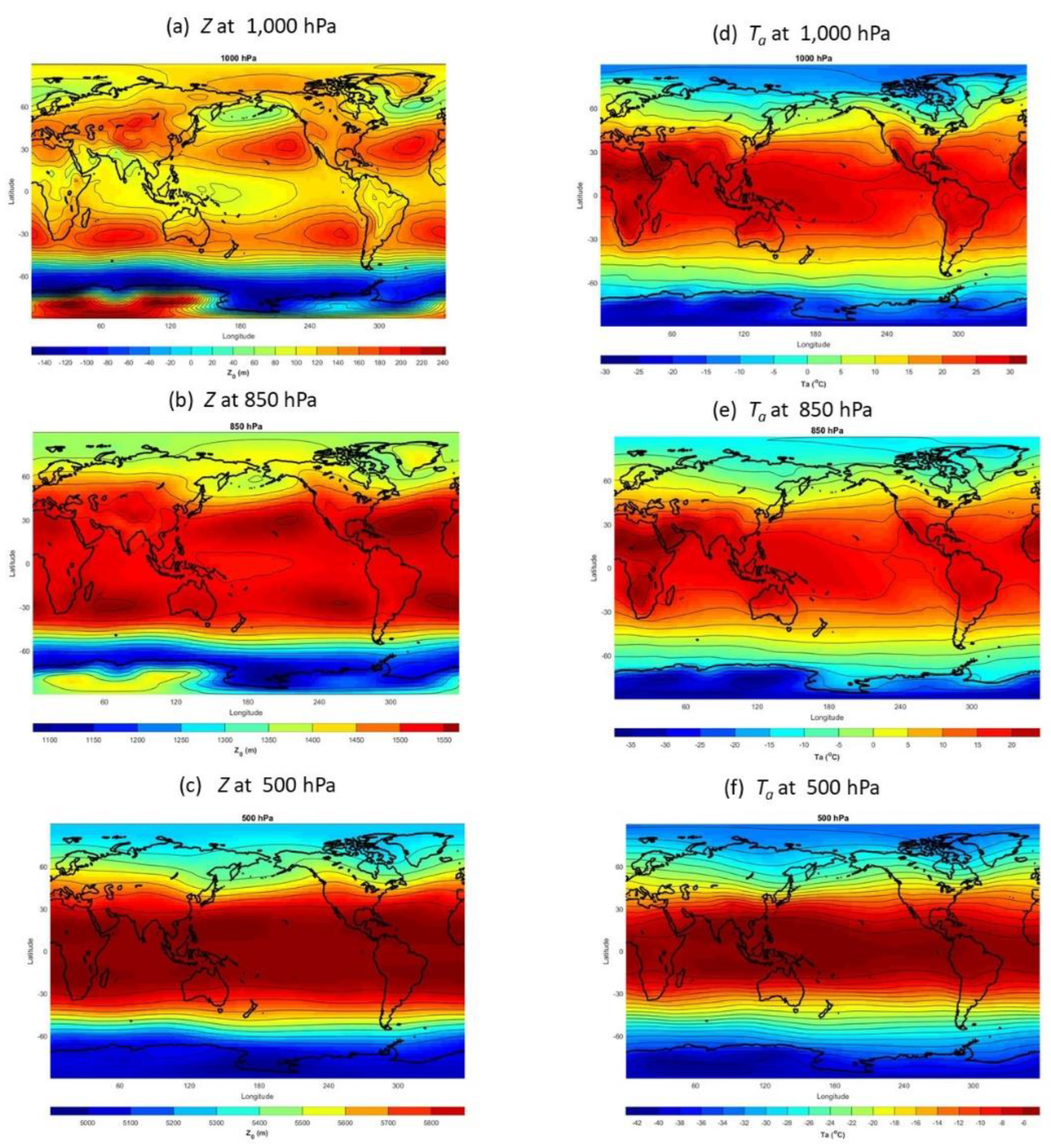
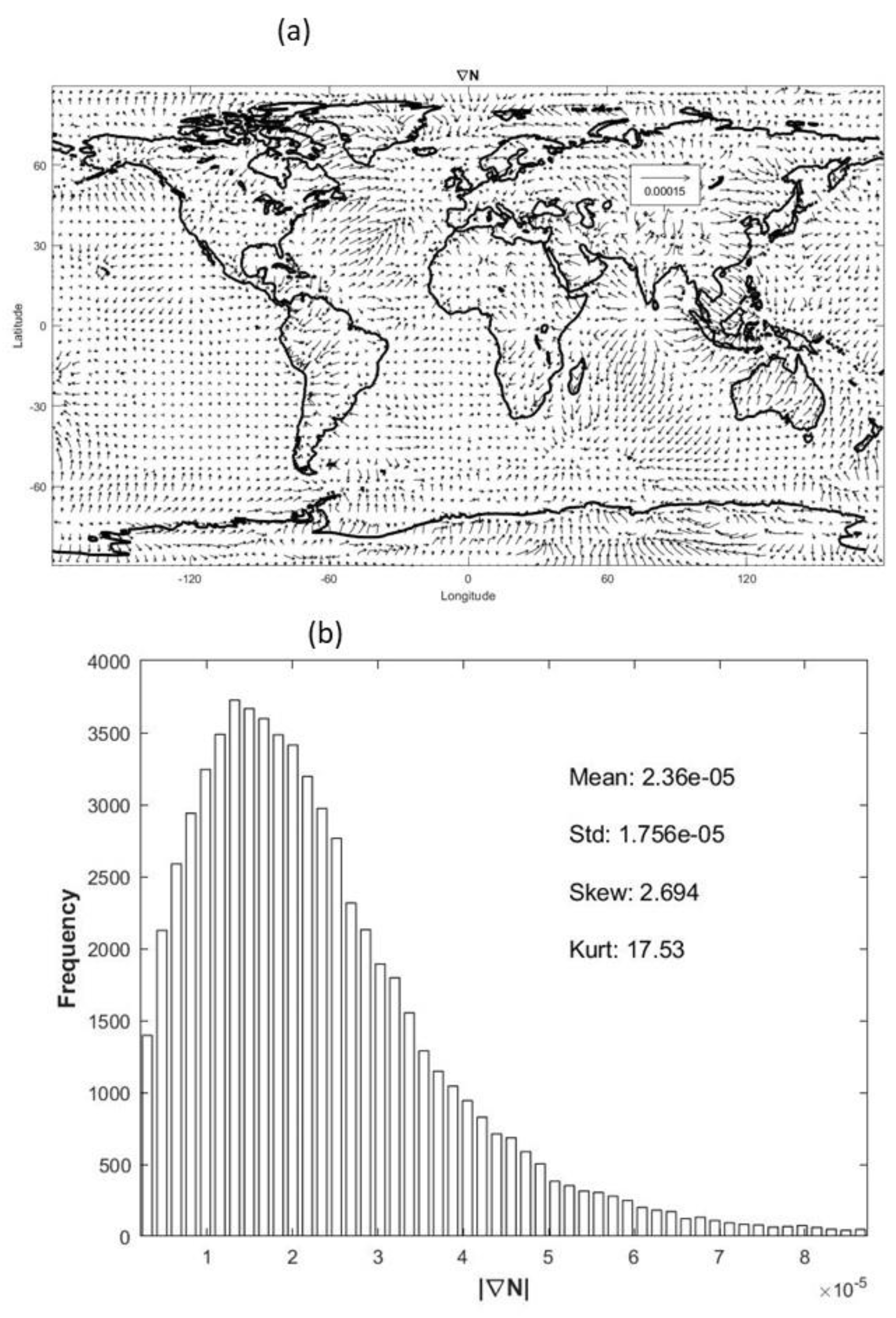
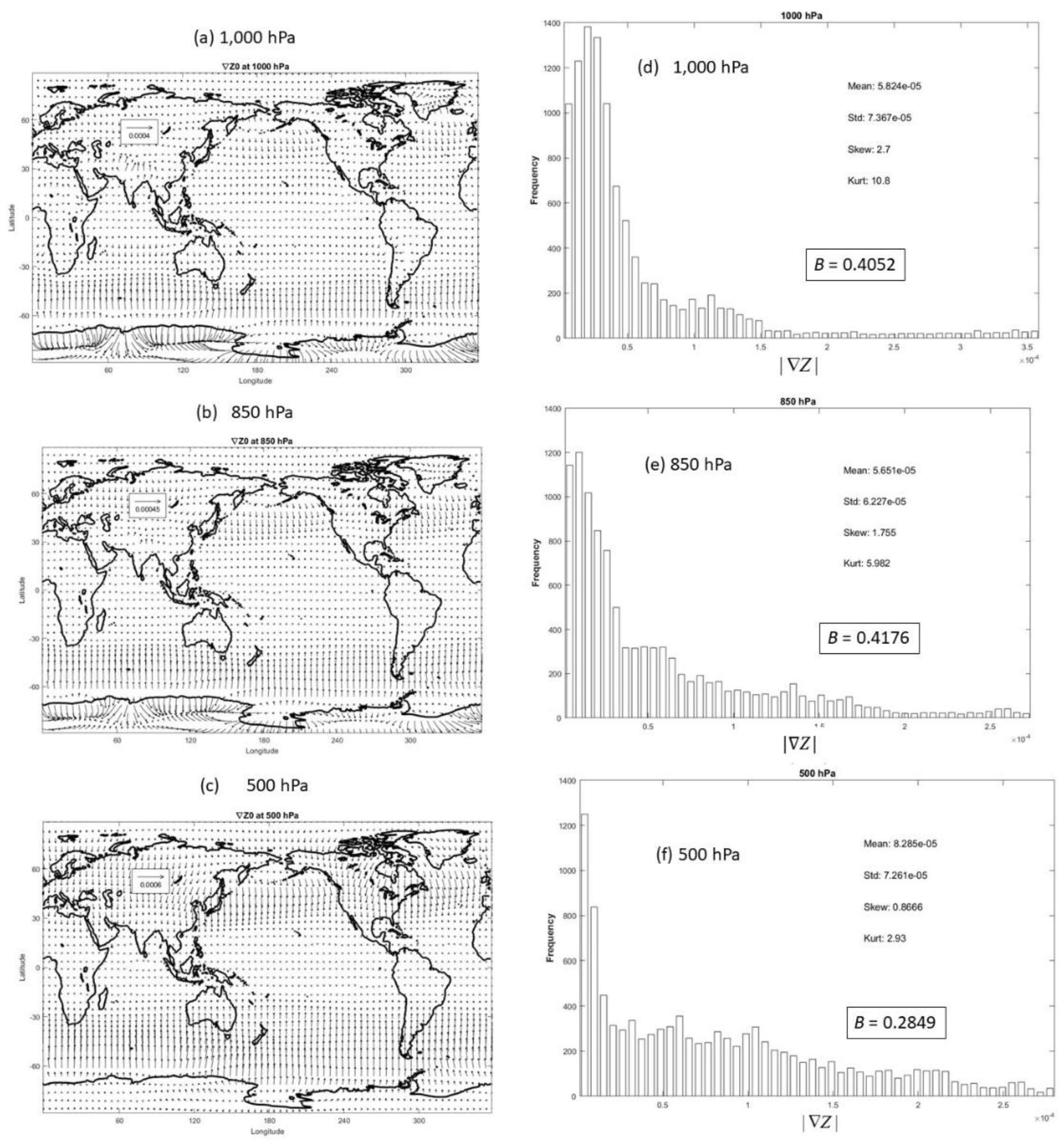
The global long-term annual mean geopotential height Z has comparable horizontal variability at 1,000 hPa (Figure 4a) as the geoid N (Figure 3a), becomes near zonal at 850 hPa (Figure 4b) and 500 hPa (Figure 4c). The vector

\nabla

_zN (Figure 5a) is

\nabla

_zT/g₀ at z = 0. The histogram of |

\nabla

_zN| (Figure 5b) shows a positively skewed distribution with a long tail and mean of 2.360

\times

10^-5. The two vector fields

\nabla

_zN (Figure 5a) and

\nabla Z

(Figures 6a-c) are quite different. The difference becomes larger as p-level decreasing from 1,000 hPa (Figure 6a) to 500 hPa (Figure 6c). The vector

\nabla Z

is near latitudinal at 500 hPa (Figure 6c). The histograms of |

\nabla Z

| show positively skewed distributions with mean of 5.824

\times

10^-5 at 1,000 hPa (Figure 6d), 5.651

\times

10^-5 at 850 hPa (Figure 6e), and 8.285

\times

10^-5 at 500 hPa (Figure 6f).

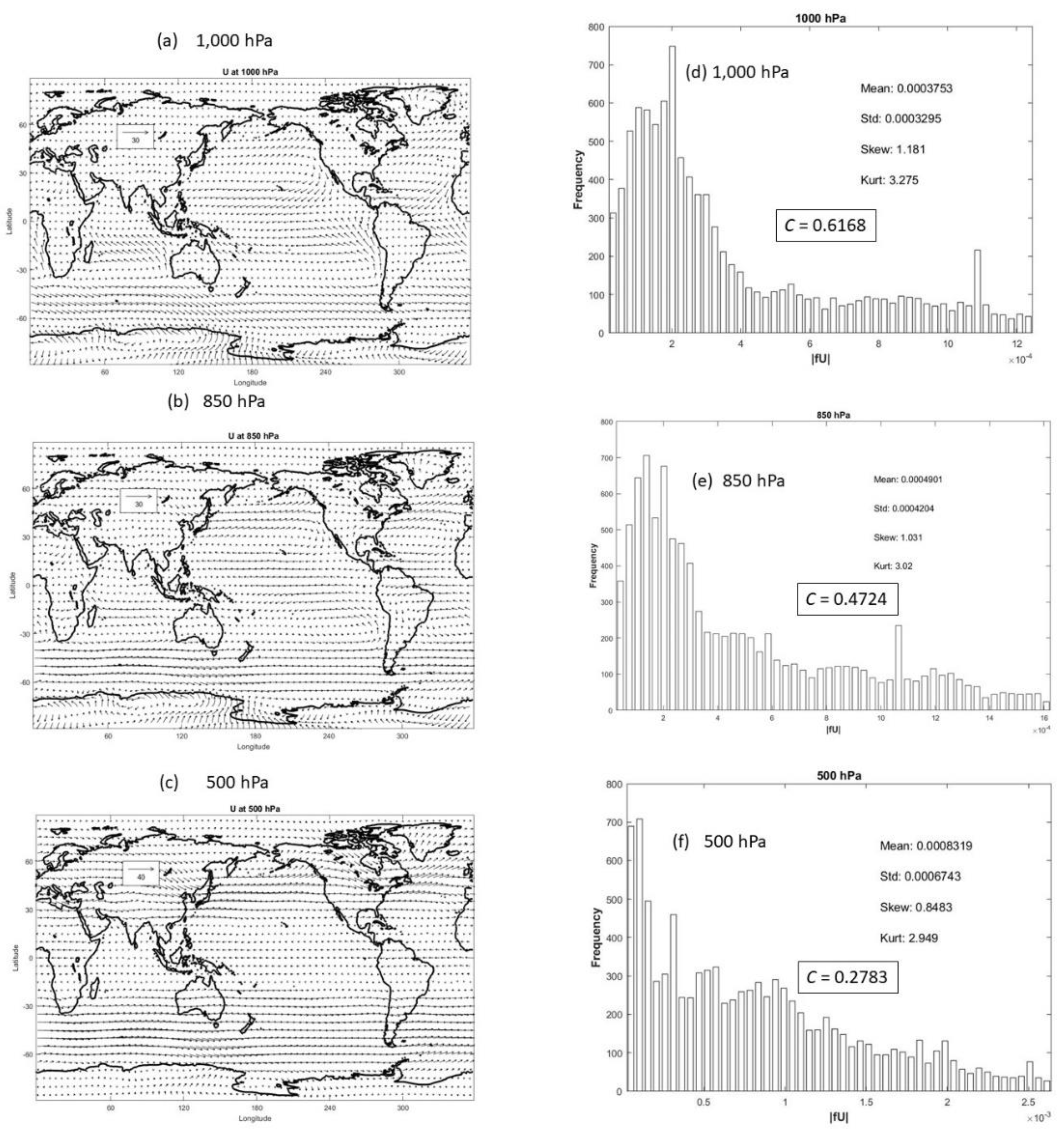
The global long-term annual mean wind vectors (U) show the general circulation at 1,000 hPa (Figure 7a), 500 hPa (Figure 7b), and 100 hPa (Figure 7c). The magnitude of the Coriolis force is represented by |fU|. The histogram of |fU| shows a positively skewed distribution with mean of 37.53 mGal at 1,000 hPa (Figure 7d), 49.01 mGal at 850 hPa (Figure 7e), and 83.19 mGal at 500 hPa (Figure 7f). The global mean of the horizontal gradient of disturbing geopotential (

\nabla

_zT = g₀

\nabla

_zN) is 23.15 mGal.

Both B and C numbers are not small. The B-number has a maximum of 0.4176 at 850 hPa and a minimum of 0.1630 at 200 hPa. It is greater than 0.28 for 1,000-500 hPa (Table 1). The C-number has a maximum of 0.6168 at 1,000 hPa, a minimum of 0.1573 at 200 hPa. It is greater than 0.27 for 1,000-500 hPa (Table 2).

3.2. Hydrostatic Equilibrium

The hydrostatic equilibrium [represented by the superscript (HE)] is defined by the coincidence of the geopotential surface with the isobaric surface. For the effective geopotential Φ_eff, we have

Φ_{e f f}^{(H E)} (or Z^{(H E)}) = const at isobaric surface \Leftrightarrow \nabla Φ_{e f f}^{(H E)} = 0 \Leftrightarrow \nabla Z^{(H E)} = 0

(32a)

For the true geopotential Φ, we get

\begin{array}{l} Φ^{(H E)} [or (Z^{(H E)} - N)] = const at isobaric surface \\ \Leftrightarrow \nabla Φ^{(H E)} = 0 \Leftrightarrow \nabla (Z^{(H E)} - N) = 0 \Leftrightarrow \nabla Z^{(H E)} = \nabla N \end{array}

(32b)

Here, Φ

\binom{(H E)}{e f f}

and Φ^(HE) are the hydrostatic equilibria of the effective and true geopotentials; Z^(HE) is the hydrostatic equilibrium of the geopotential height. Obviously, the hydrostatic equilibrium is different between the effective geopotential (Φ_eff) and the true geopotential (Φ).

3.3. Geostrophic Wind

Steady state flow without friction leads to the geostrophic balance from Eq.(27)

f k \times U_{g} = - \nabla Φ_{e f f} + \nabla T

(33)

which is rewritten by

U_{g} = \frac{k}{f} \times [\nabla Φ_{e f f} - \nabla T]

(34)

The geostrophic wind is decomposed into two parts, U_g = U_g0 + U_gδ, with

U_{g 0} = \frac{k}{f} \times \nabla Φ_{e f f} = \frac{g_{0}}{f} k \times \nabla Z

(35)

which represents the classical geostrophic wind, and

U_{g δ} = - \frac{k}{f} \times \nabla T \approx - \frac{g_{0} k}{f} \times \nabla N

(36)

which denotes the geostrophic wind due to the gravity disturbance vector δg. Obviously, the non-dimensional B number (31) is also the ratio between O(|U_gδ|) and O(|U_g0|),

\begin{array}{l} \frac{O (| U_{g δ} |)}{O [| U_{g 0} |]} = \frac{g_{0} O (| \nabla_{z} N |)}{O (| \nabla Φ_{e f f} |)} = \frac{O (| \nabla_{z} N |)}{O (| \nabla Z |)} = \frac{mean (| \nabla_{z} N |)}{mean (| \nabla Z |)} \\ = B = {\begin{matrix} 0.4176 (\max) at 850 hPa \\ 0.1630 (\min) at 200 hPa \end{matrix} \end{array}

(37)

The B number listed in Table 1 from 1,000 hPa to 100 hPa demonstrates that the gravity disturbance vector (δg) is nonnegligible in the geostrophic wind.

3.4. Thermal Wind

Differentiation of the geostrophic wind equation (34) with respect to p leads to

\frac{\partial U_{g}}{\partial p} = \frac{k}{f} \times [\nabla (\frac{\partial Φ_{e f f}}{\partial p}) - \nabla (\frac{\partial T}{\partial p})]

(38)

Since

\frac{\partial T}{\partial p} = \frac{\partial T / \partial z}{\partial p / \partial z} = - \frac{\partial T / \partial z}{ρ g_{0}}, \frac{\partial Φ_{e f f}}{\partial p} = - \frac{1}{ρ}, ρ = \frac{p}{R_{a} T_{a}}

(39)

substitution of (39) into (38) leads to

\frac{\partial U_{g}}{\partial p} = \frac{k}{f} \times [\nabla (- \frac{R_{a} T_{a}}{p})] (1 - \frac{T_{z}}{g_{0}}) + \frac{R_{a} T_{a}}{p} \frac{k}{f} \times \nabla (\frac{T_{z}}{g_{0}})

(40)

where R_a = 287 JK^-1kg^-1, is the gas constant for dry air. Since |T_z|/g₀ < 5.443×10^-4 [see Eq.(24)] and should be neglected against 1. Eq.(40) becomes

\frac{\partial U_{g}}{\partial \ln p} = = - \frac{R_{a} k}{f} \times \nabla T_{a} + \frac{R_{a} T_{a}}{g_{0}} \frac{k}{f} \times \nabla T_{z}

(41)

The nondimensional A number is defined by

A = \frac{O [| \nabla T_{z} | / g_{0}]}{O [| \nabla T_{a} | / T_{a}]} \approx \frac{O [| \nabla_{z} T_{z} | / g_{0}]}{O [| \nabla T_{a} | / T_{a}]}

(42)

to identify relative importance of the gravity disturbance vector (δg) versus the effective gravity (g_eff) on the thermal wind relation.

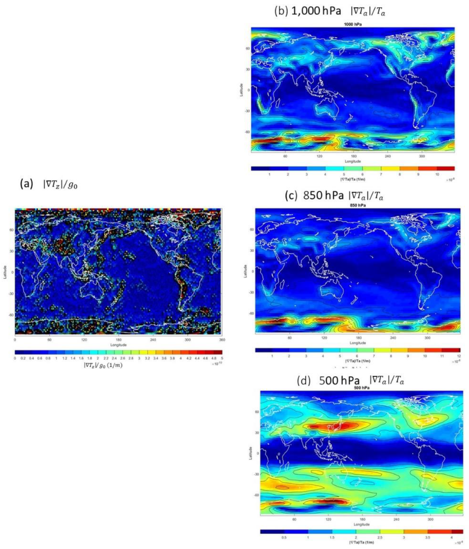
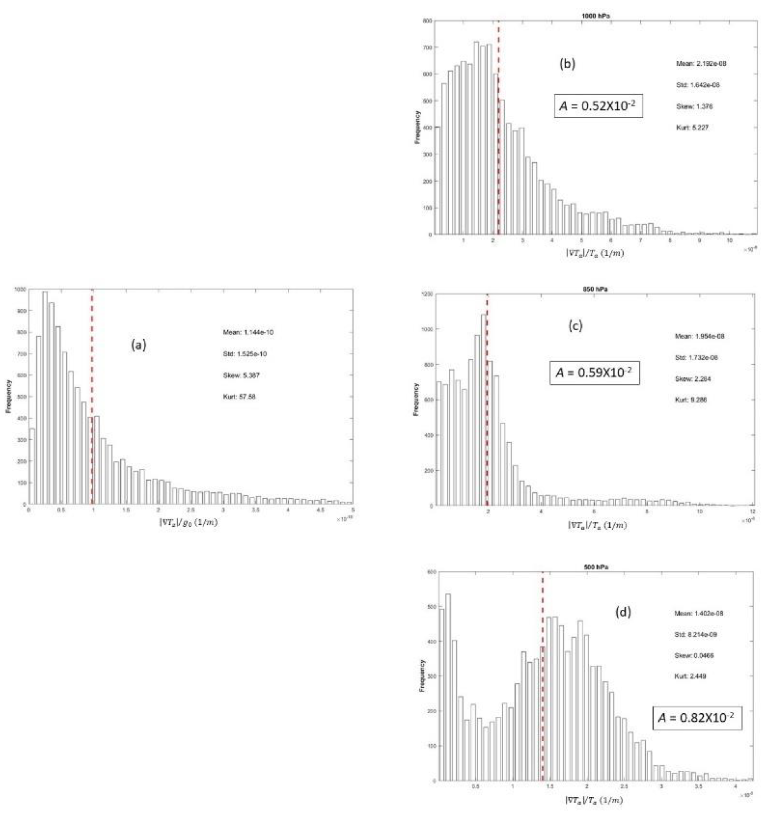
The variable

| \nabla

_zT_z|/g₀ is calculated from the static gravity field model EIGEN-6C4 T_z data (Figure 8a). The variable

| \nabla

T_a|/T_a is computed from the NCEP/NCAR reanalyzed global long-term annual mean air temperature T_a at 12 pressure levels such as at 1,000 hPa (Figure 8b), 850 hPa (Figure 8c), and 500 hPa (Figure 8d). The histogram of

| \nabla

_zT_z|/g₀ shows a positively skewed distribution with the mean of 1.144×10^-10m^-1 (Figure 9a). The histograms of^.

| \nabla

T_a|/T_a also show positively skewed distributions with the mean of 2.192×10^-8m^-1 at 1,000 hPa (Figure 9b), with the mean of 1.954×10^-8m^-1 at 850 hPa (Figure 9c), and a bi-modal distribution with the mean of 1.402×10^-8m^-1 at 500 hPa (Figure 9d). The A number varies from 0.5219×10^-2 (min) at 1,000 hPa to 1.9816×10^-2 (max) at 200 hPa (Table 3). Such small values of the A number demonstrate the second term in the righthand side of (41) negligible,

\frac{\partial U_{g}}{\partial \ln p} = - \frac{R_{a} k}{f} \times \nabla T_{a}

(43)

which leads to

\frac{\partial Φ}{\partial p} = \frac{\partial Φ_{e f f}}{\partial p} = - \frac{R_{a} T_{a}}{p}

(44)

which indicates that the thermal wind relation is kept unchanged from using the effective geopotential Φ_eff to the true geopotential Φ. This is caused by that the disturbing gravity potential at the surface (z =0), T(λ, φ, 0), and its z-derivative T_z(λ, φ, 0) are used approximately for the whole troposphere, see Equation (15).

3.5. Geostrophic Vorticity

In p as the vertical coordinate and the Coriolis parameter taken as a constant, the geostrophic relative vorticity is given by

ζ_{e f f} = \frac{1}{f} \nabla^{2} Φ_{e f f}

(45a)

with the effective gravity (g_eff) and is represented by

ζ = \frac{1}{f} \nabla^{2} Φ = ζ_{e f f} + ζ_{g d}, ζ_{e f f} = \frac{1}{f} \nabla^{2} Φ_{e f f} = \frac{g_{0}}{f} \nabla^{2} Z, ζ_{g d} = - \frac{g_{0}}{f} \nabla^{2} N

(45b)

with the true gravity (g). Here, Eq.(17) is used and ζ_gd represents the geostrophic vorticity due to the gravity disturbance vector (δg).

3.6. Ekman Pumping

The Ekman pumping velocity at the top of the Ekman layer is given by [1] (P132, Equation 5.38)

w (D_{E}) = \frac{ζ}{2 γ} = \frac{1}{2 γ} (ζ_{e f f} + ζ_{g d}), γ \equiv {| \frac{f}{2 K} |}^{1 / 2} (\frac{f}{| f |})

(46)

A nondimensional D number is defined by

D \equiv \frac{O (| ζ_{g d} |)}{O (| ζ_{e f f} |)} = \frac{O [| \nabla^{2} N |]}{O [| \nabla^{2} Z |]} \approx \frac{O [| \nabla_{z}^{2} N |]}{O [| \nabla^{2} Z |]}

(47)

to identify relative importance of δg versus the effective gravity (g_eff) on the geostrophic vorticity and in turn on the Ekman layer dynamics.

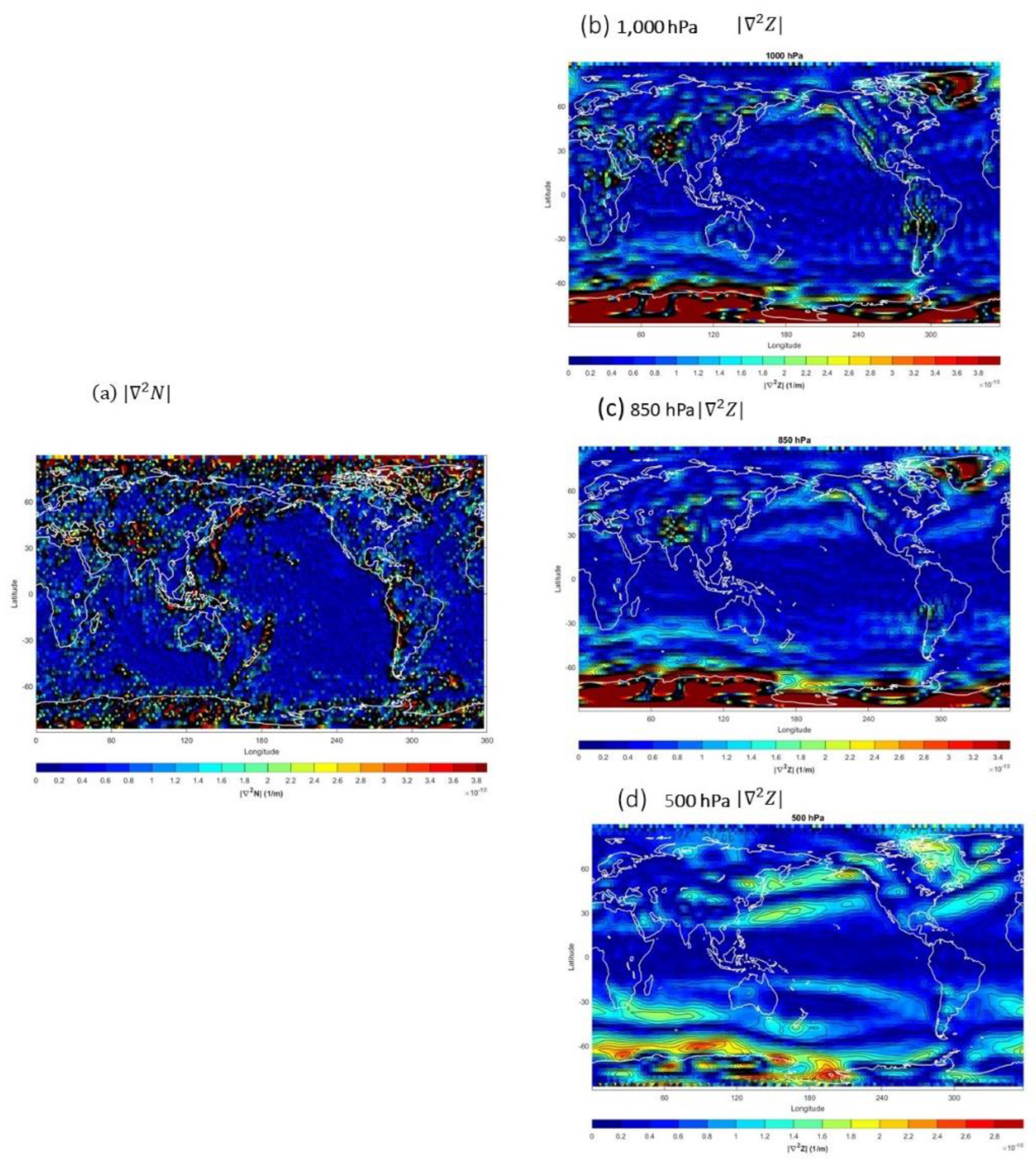
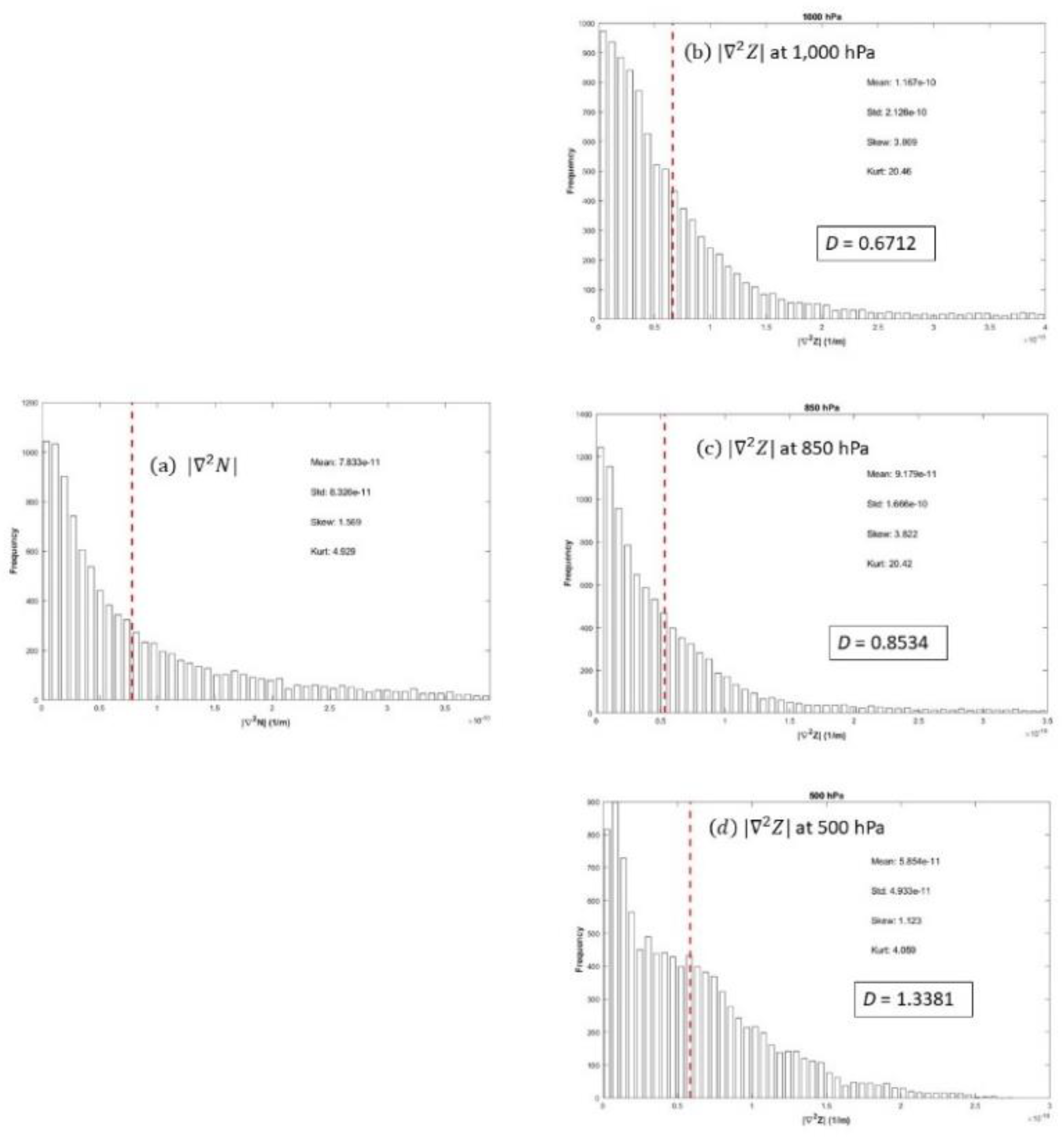
The static gravity field model EIGEN-6C4 N data are used to calculate |

\nabla \binom{2}{z}

N| (Figure 10a). The NCEP/NCAR reanalyzed global long-term annual mean geopotential height Z data are used to compute

| \nabla

²Z| for 12 pressure levels such as 1,000 hPa (Figure 10b), 850 hPa (Figure 10c), and 500 hPa (Figure 10d). The histogram of |

\nabla \binom{2}{z}

N| shows a positively skewed distribution with the mean of 0.7833×10^-10m^-1 (Figure 11a). The histograms of^.

| \nabla

²Z| also show positively skewed distributions with the mean of 1.167×10^-10m^-1 at 1,000 hPa (Figure 11b), with the mean of 0.9179×10^-10m^-1 at 850 hPa (Figure 11c), and with the mean of 0.5854×10^-10m^-1 at 500 hPa (Figure 11d). The D number varies from 0.6712 (min) at 1,000 hPa to 1.3381 (max) at 500 hPa (Table 4). Such values of the D number demonstrate the gravity disturbance vector (δg) is non-negligible in comparison to the effective gravity (g_eff) on the geostrophic vorticity. Besides, if 850 hPa is treated as the top of the Ekman layer, the Ekman pumping velocity (proportional to the geostrophic vorticity) is comparable due to the effective geopotential

\nabla

²Z and due to the gravity disturbance vector

\nabla \binom{2}{z}

N because B = 0.8534 at 850 hPa.

3.7. Q vector

The Q vector defined by [1] (P170, Equation 6.54)

Q \equiv (Q_{1}, Q_{2}) = (- \frac{R_{a}}{p} \frac{\partial U_{g}}{\partial x} • \nabla T_{a}, - \frac{R_{a}}{p} \frac{\partial U_{g}}{\partial y} • \nabla T_{a})

(48)

is used in atmospheric dynamics to identify physical processes such as vertical motion and frontogenesis on the base of the quasi-geostrophic system. Here, (x, y) are local horizontal coordinates. Substitution of (34) into (48) leads to

Q = Q^{e f f} + Q^{g d}, Q^{e f f} = (Q_{1}^{e f f}, Q_{2}^{e f f}), Q^{g d} = (Q_{1}^{g d}, Q_{2}^{g d})

(49)

where Q^eff and Q^gd are the Q vector associated with the effective gravity and gravity disturbance vector, respectively. Their components are given by

\begin{array}{l} Q_{1}^{e f f} = - \frac{R_{a}}{p} \frac{\partial U_{g 0}}{\partial x} • \nabla T_{a} = - \frac{R_{a} g_{0}}{p f} q_{1}^{e f f}, Q_{2}^{e f f} = - \frac{R_{a}}{p} \frac{\partial U_{g 0}}{\partial y} • \nabla T_{a} = - \frac{R_{a} g_{0}}{p f} q_{2}^{e f f} \\ Q_{1}^{g d} = - \frac{R_{a}}{p} \frac{\partial U_{g δ}}{\partial x} • \nabla T_{a} = \frac{R_{a} g_{0}}{p f} q_{1}^{g d}, Q_{2}^{g d} = - \frac{R_{a}}{p} \frac{\partial U_{g δ}}{\partial y} • \nabla T_{a} = \frac{R_{a} g_{0}}{p f} q_{2}^{g d} \end{array}

(50)

where

q_{1}^{e f f} = - J (\frac{\partial Z}{\partial x}, T_{a}), q_{2}^{e f f} = - J (\frac{\partial Z}{\partial y}, T_{a}), q_{1}^{g d} = J (\frac{\partial N}{\partial x}, T_{a}), q_{2}^{g d} = J (\frac{\partial N}{\partial y}, T_{a})

(51)

are the components of two vectors q^eff =

(q \binom{e f f}{1}

q \binom{e f f}{2}),

q^gd =

(q \binom{g d}{1}

q \binom{g d}{2}),

and J(V,W) ≡ (∂V/∂x)(∂W/∂y) - (∂W/∂x)(∂V/∂y) is the Jacobian. Two non-dimensional number (E₁, E₂) are defined by

E_{1} \equiv \frac{O (| q_{1}^{g d} |)}{O (| q_{1}^{e f f} |)} = \frac{O (| J (\frac{\partial N}{\partial x}, T_{a}) |)}{O (| J (\frac{\partial Z}{\partial x}, T_{a}) |)}, E_{2} \equiv \frac{O (| q_{2}^{g d} |)}{O (q_{2}^{e f f})} = \frac{O (| J (\frac{\partial N}{\partial y}, T_{a}) |)}{O (| J (\frac{\partial Z}{\partial y}, T_{a}) |)}

(52)

to identify relative importance of gravity disturbance vector (δg) versus the effective gravity (g_eff) on the two components of the Q vector.

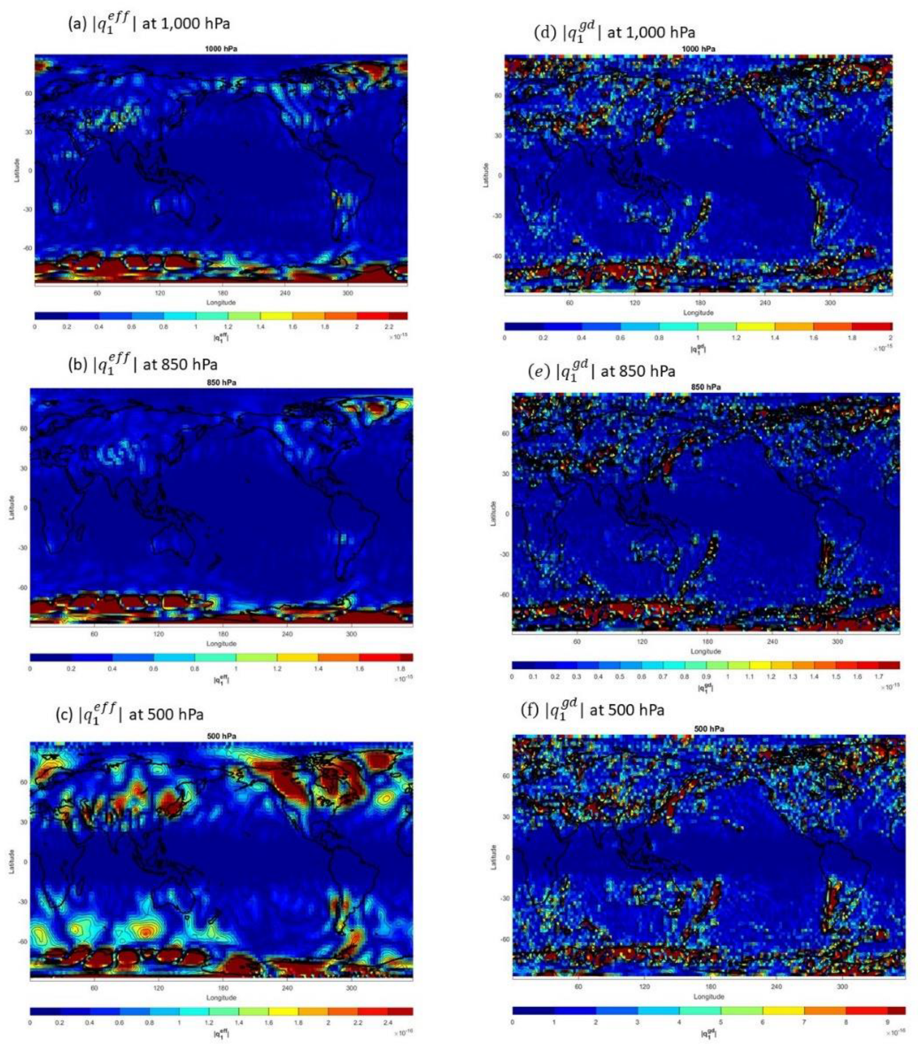
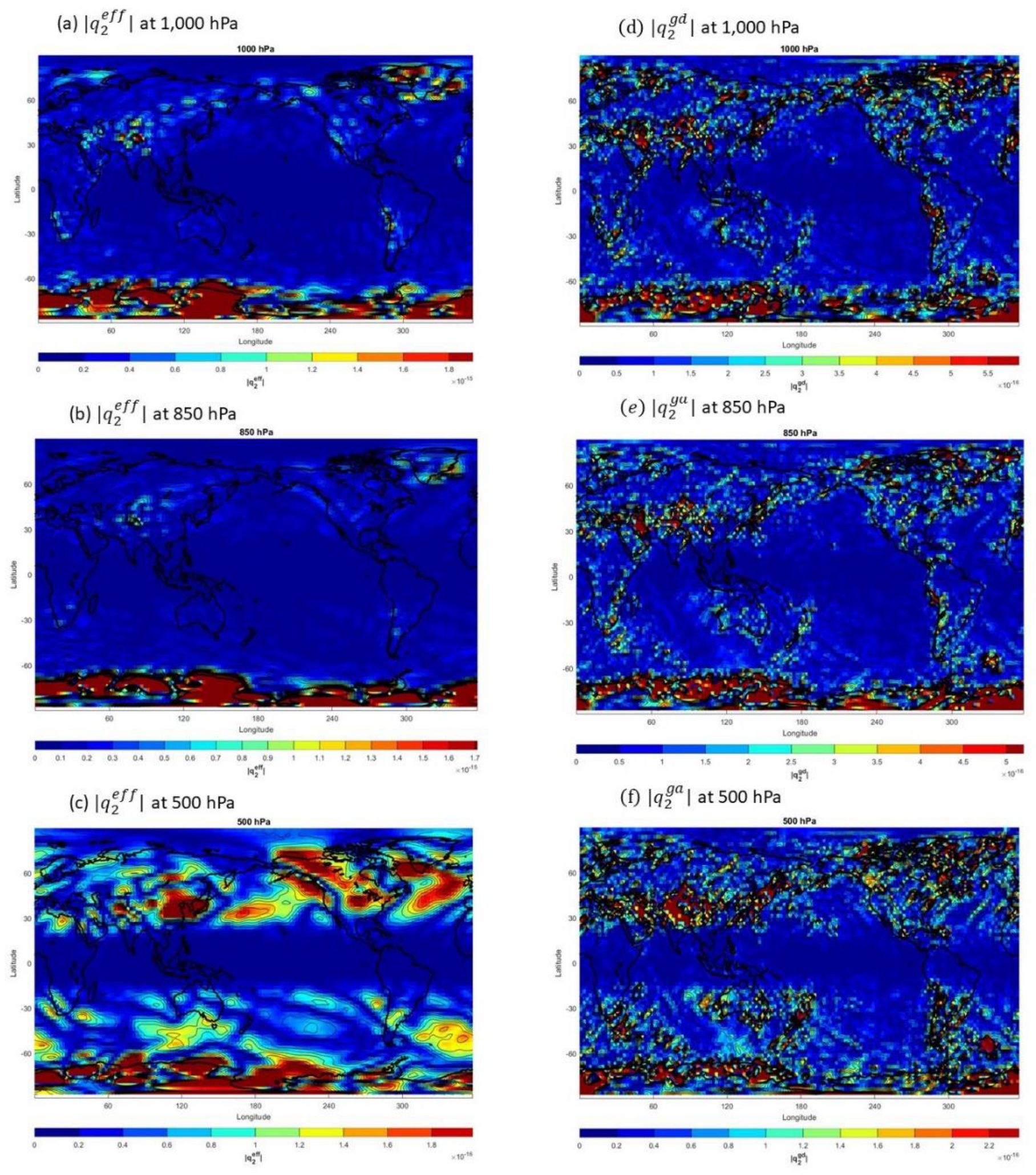
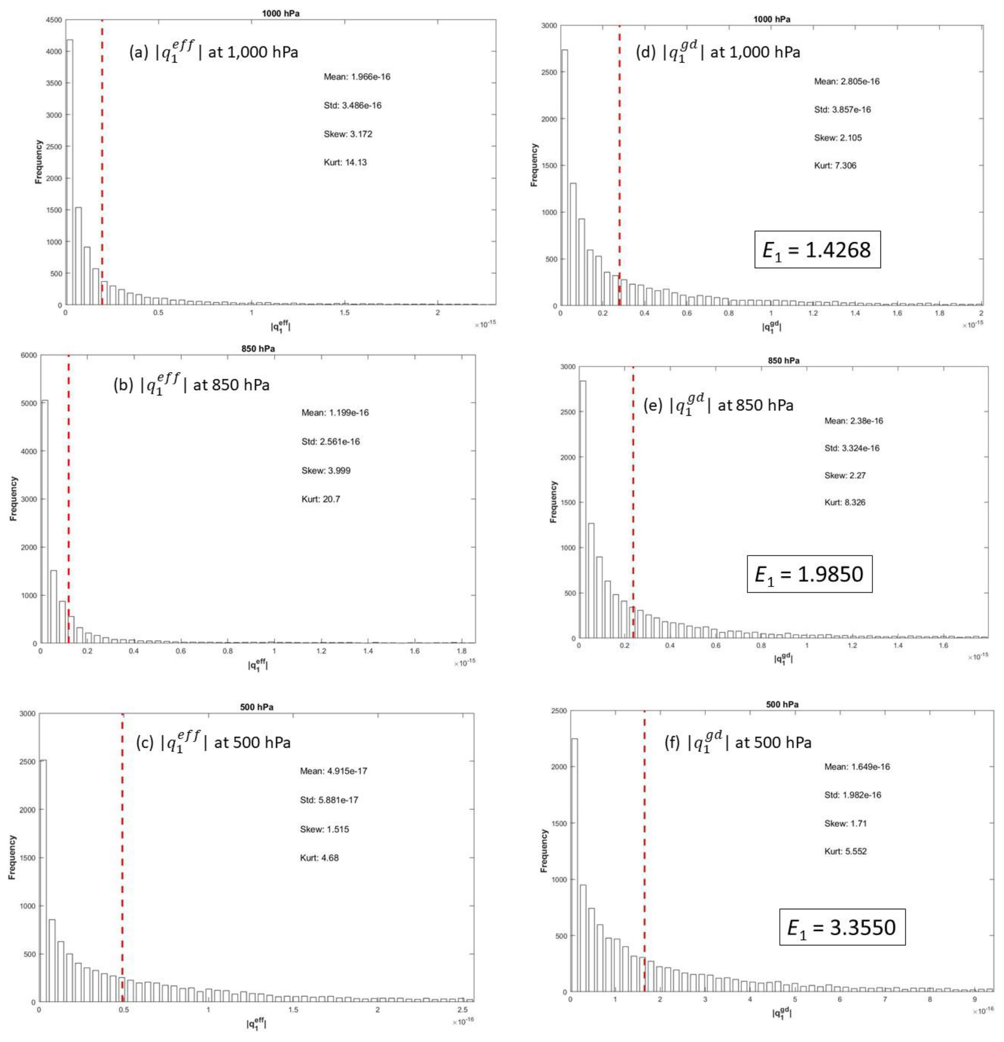
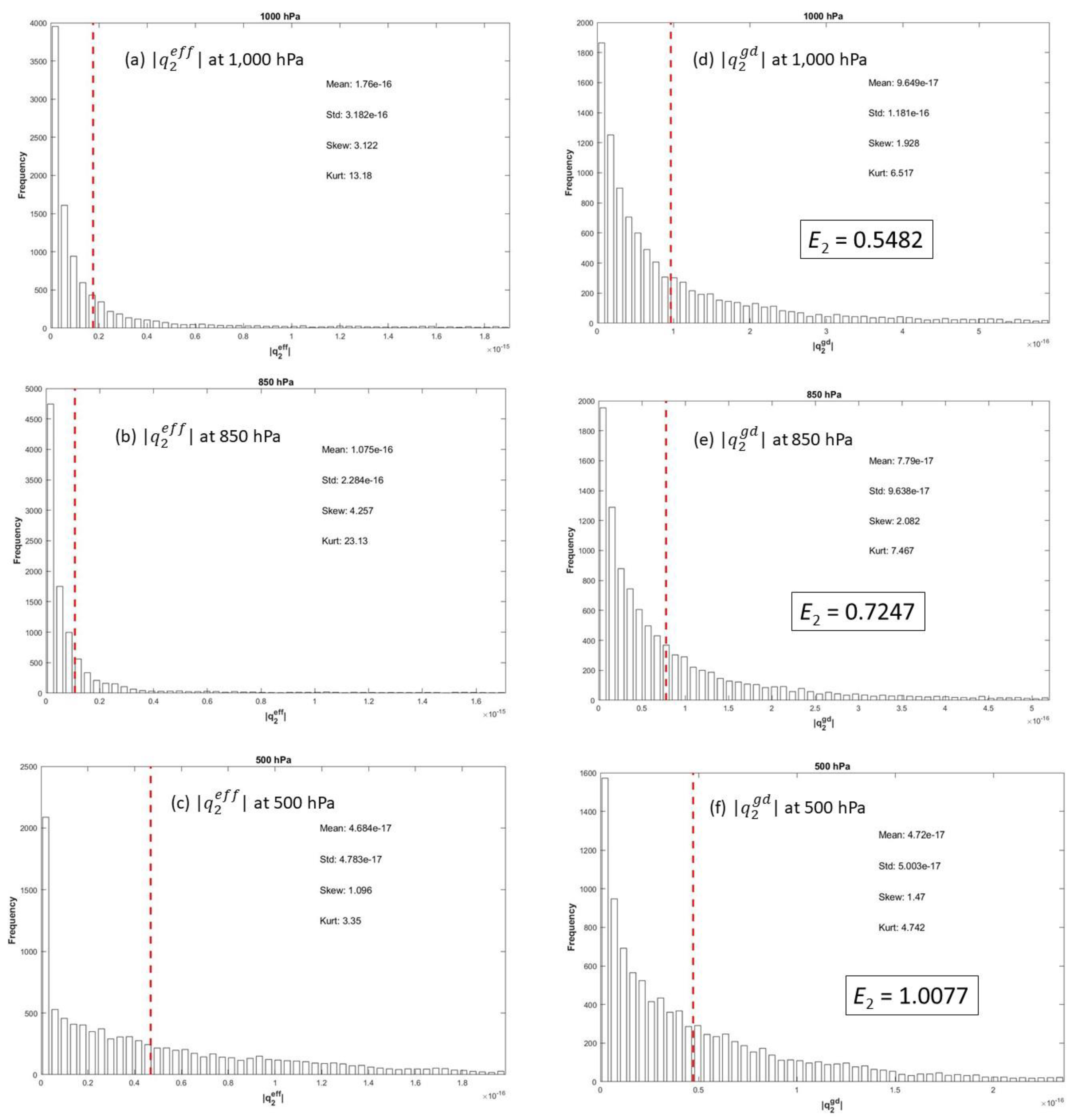
The NCEP/NCAR reanalyzed global long-term annual mean geopotential height (Z) and temperature (T_a) are used to calculate

| q \binom{e f f}{1} |

at 1,000 hPa (Figure 12a), 850 hPa (Figure 12b), and 500 hPa (Figure 12c) and

| q \binom{e f f}{2} |

at 1,000 hPa (Figure 13a), 850 hPa (Figure 13b), and 500 hPa (Figure 13c). The static gravity field model EIGEN-6C4 (for N) and NCEP/NCAR reanalyzed global long-term annual mean temperature (T_a) are used to calculate

| q \binom{g d}{1} |

at 1,000 hPa (Figure 12d), 850 hPa (Figure 12e), and 500 hPa (Figure 12f) and

| q \binom{g d}{2} |

at 1,000 hPa (Figure 13d), 850 hPa (Figure 13e), and 500 hPa (Figure 13f). The histograms of^.

| q \binom{e f f}{1} |

show positively skewed distributions with the mean of 1.966×10^-16m^-1 at 1,000 hPa (Figure 14a), 1.199×10^-16m^-1 at 850 hPa (Figure 14b), and 0.4915×10^-16m^-1 at 500 hPa (Figure 14c). The histograms of^.

| q \binom{g d}{1} |

show positively skewed distributions with the mean of 2.805×10^-16m^-1 at 1,000 hPa (Figure 14d), 2.380×10^-16m^-1 at 850 hPa (Figure 14e), and 1.649×10^-16m^-1 at 500 hPa (Figure 14f). The E₁ number varies from 1.4268 (min) at 1,000 hPa to 4.3834 (max) at 100 hPa (Table 5). Similarly, the histograms of^.

| q \binom{e f f}{2} |

show positively skewed distributions with the mean of 1.760×10^-16m^-1 at 1,000 hPa (Figure 15a), 1.075×10^-16m^-1 at 850 hPa (Figure 15b), and 0.4684×10^-16m^-1 at 500 hPa (Figure 15c). The histograms of^.

| q \binom{g d}{2} |

show positively skewed distributions with the mean of 0.9649×10^-16m^-1 at 1,000 hPa (Figure 15d), 0.7790×10^-16m^-1 at 850 hPa (Figure 15e), and 0.4720×10^-16m^-1 at 500 hPa (Figure 15f). The E₂ number varies from 0.5482 (min) at 1,000 hPa to 1.057 (max) at 600 hPa (Table 6). It clearly demonstrates that the effect of δg is important in the Q vector.

Table 5. Global means of

| q \binom{g d}{1} |

and annual

| q \binom{e f f}{1} |

at 12 pressure levels in the troposphere (treated as the order of magnitude) as well as the non-dimensional E₁-number.

Table 5. Global means of

| q \binom{g d}{1} |

and annual

| q \binom{e f f}{1} |

at 12 pressure levels in the troposphere (treated as the order of magnitude) as well as the non-dimensional E₁-number.

Pressure Level (hPa)	$Mean (\| q \binom{e f f}{1}$ ) (10^-16 m^-1)	$Mean (\| q \binom{g d}{1} \|$ ) (10^-16 m^-1)	E₁-number
1,000	1.966	2.805	1.4268
925	1.516	2.533	1.6708
850	1.199	2.380	1.9850
700	0.7411	2.121	2.8620
600	0.5468	1.814	3.3175
500	0.4915	1.649	3.3550
400	0.4553	1.508	3.3121
300	0.3765	1.130	3.0013
250	0.2813	0.9059	3.2204
200	0.2023	0.6462	3.1943
150	0.2630	0.9091	3.4567
100	0.3203	1.404	4.3834

Table 6. Global means of

| q \binom{g d}{2} |

and annual

| q \binom{e f f}{2} |

at 12 pressure levels in the troposphere (treated as the order of magnitude) as well as the non-dimensional E₂-number.

Table 6. Global means of

| q \binom{g d}{2} |

and annual

| q \binom{e f f}{2} |

at 12 pressure levels in the troposphere (treated as the order of magnitude) as well as the non-dimensional E₂-number.

Pressure Level (hPa)	$Mean (\| q \binom{e f f}{2} \|$ ) (10^-16 m^-1)	$Mean (\| q \binom{g d}{2} \|$ ) (10^-16 m^-1)	E₂-number
1,000	1.760	0.9649	0.5482
925	1.381	0.8569	0.6205
850	1.075	0.7790	0.7247
700	0.6787	0.6174	0.9097
600	0.4948	0.5230	1.0570
500	0.4684	0.4720	1.0077
400	0.4614	0.4335	0.9395
300	0.4359	0.3527	0.8091
250	0.3704	0.2884	0.7786
200	0.3116	0.2128	0.6829
150	0.3628	0.2826	0.7789
100	0.4330	0.4315	0.9965

3.8. Omega Equation

The quasi-geostrophic Omega equation on the f-plane given by [1] (P.170, Equation 6.53)

σ \nabla^{2} ω + f^{2} \frac{\partial^{2} ω}{\partial p^{2}} = - 2 \nabla • Q - \frac{κ}{p} \nabla^{2} J

(53)

is used to diagnose the large-scale atmospheric vertical motion. Here, κ = R/c_p, c_p is the specific heat; and J is the rate of heating per unit mass due to radiation, conduction, and latent heat release. Substitution of (49) into (53) leads to

σ \nabla^{2} ω + f^{2} \frac{\partial^{2} ω}{\partial p^{2}} = - 2 \nabla • Q^{e f f} - 2 \nabla • Q^{g d} - \frac{κ}{p} \nabla^{2} J

(54)

Substitution of (50) into (54) leads to

\nabla • Q^{e f f} = \frac{R_{a} g_{0}}{p f} \nabla • q^{e f f}, \nabla • Q^{g d} = \frac{R_{a} g_{0}}{p f} \nabla • q^{g d}

(55)

Substitution of (51) into (55) gives

\nabla • q^{e f f} = J (\nabla^{2} Z, T_{a}) + J (\partial Z / \partial x, \partial T_{a} / \partial x) + J (\partial Z / \partial y, \partial T_{a} / \partial y)

(56)

\nabla • q^{g d} = J (\nabla^{2} N, T_{a}) + J (\partial N / \partial x, \partial T_{a} / \partial x) + J (\partial N / \partial y, \partial T_{a} / \partial y)

(57)

A non-dimensional E₃ number is defined by

E_{3} \equiv \frac{O (| \nabla • Q^{g d} |)}{O (| \nabla • Q^{e f f} |)} = \frac{O (| \nabla • q^{g d} |)}{O (| \nabla • q^{e f f} |)}

(58)

to identify relative importance of gravity disturbance vector (δg) versus the effective gravity (g_eff) on the Omega equation.

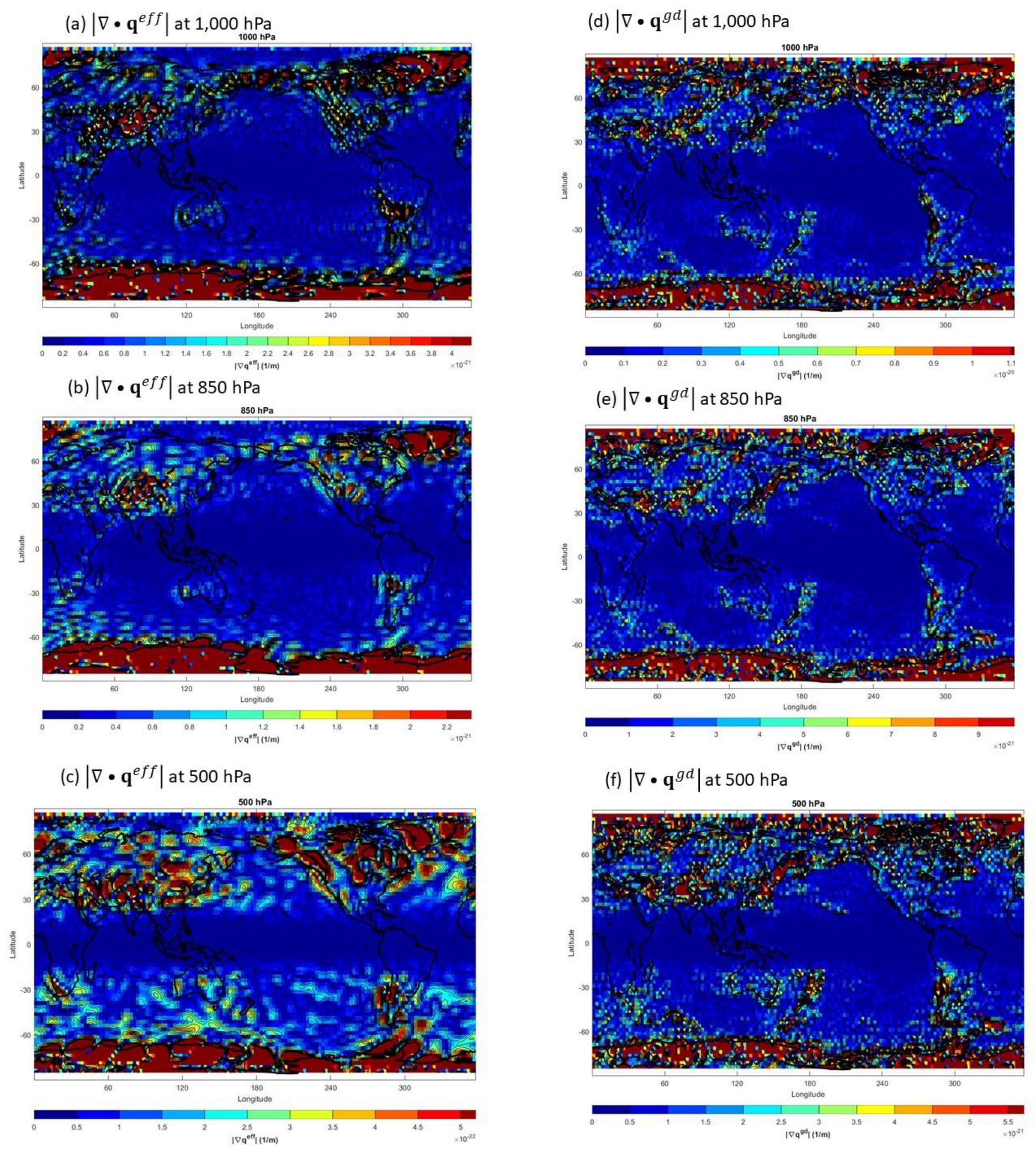
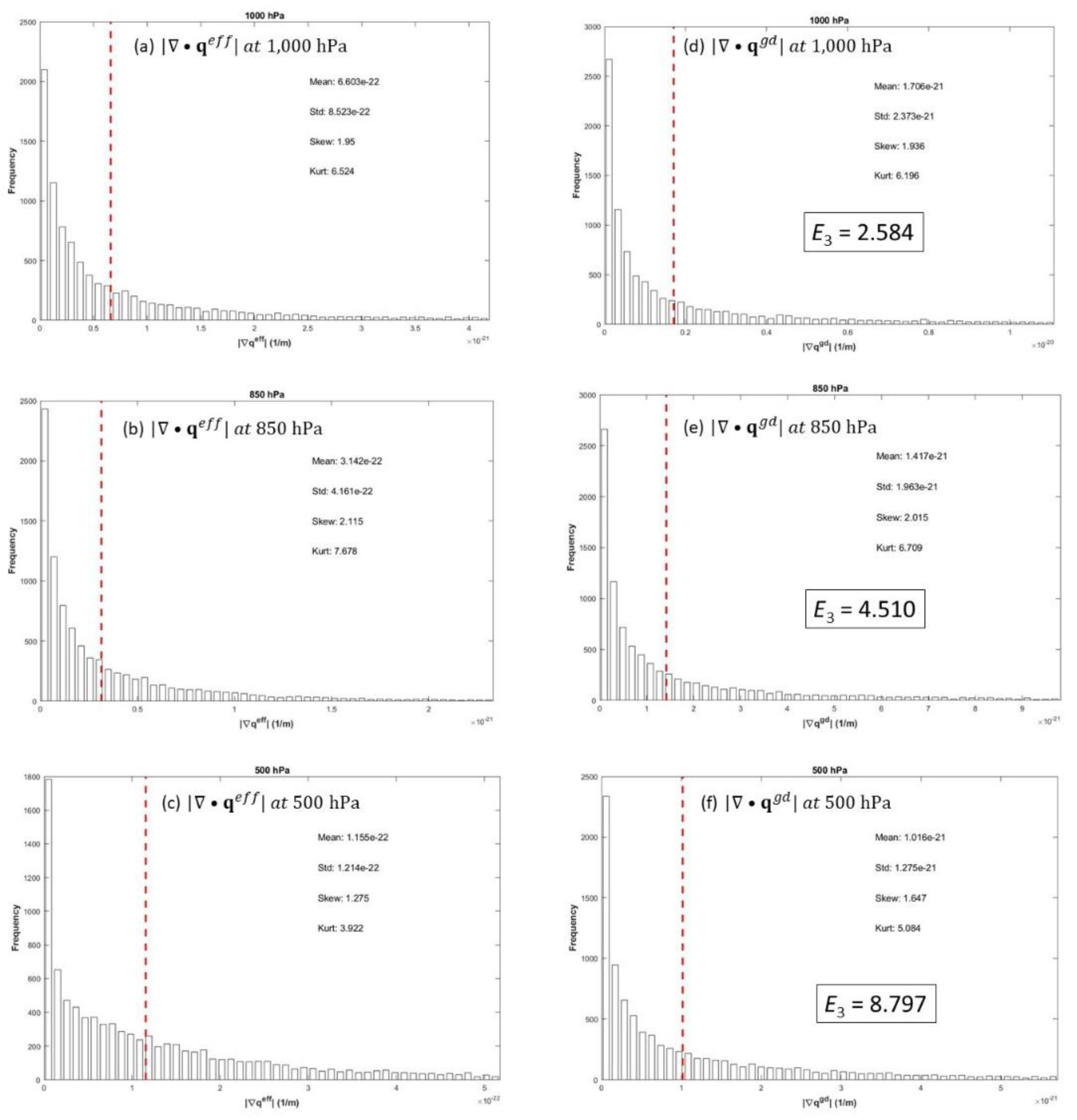
The NCEP/NCAR reanalyzed global long-term annual mean geopotential height (Z) and temperature (T_a) are used to calculate

| \nabla • q

^eff| at 1,000 hPa (Figure 16a), 850 hPa (Figure 16b), and 500 hPa (Figure 16c). The static gravity field model EIGEN-6C4 (for N) and NCEP/NCAR reanalyzed global long-term annual mean temperature (T_a) are used to calculate

| \nabla • q

^gd| at 1,000 hPa (Figure 16d), 850 hPa (Figure 16e), and 500 hPa (Figure 16f). The histograms of^.

| \nabla • q

^eff| show positively skewed distributions with the mean of 6.603×10^-22m^-1 at 1,000 hPa (Figure 17a), 3.142×10^-22m^-1 at 850 hPa (Figure 17b), and 1.156×10^-22m^-1 at 500 hPa (Figure 17c). The histograms of^.

| \nabla • q

^gd| show positively skewed distributions with the mean of 17.06×10^-22m^-1 at 1,000 hPa (Figure 17d), 14.17×10^-22m^-1 at 850 hPa (Figure 17e), and 10.16×10^-22m^-1 at 500 hPa (Figure 17f). The E₃ number varies from 2.584 (min) at 1,000 hPa to 11.713 (max) at 100 hPa (Table 7). It clearly demonstrates that the importance of δg in comparison to the effective gravity (g_eff) in the Omega equation.

4. Discussion

The effective gravity g_eff used in large-scale atmospheric dynamics and modeling is untrue since it is obtained from shrinking the Earth into a point-mass with entire mass concentrated at the Earth center. The true gravity g minus the effective gravity g_eff is the gravity disturbance vector δg (δg = g – g_eff). The effect of δg in atmospheric dynamics is studied through replacing g_eff by g. Seven non-dimensional numbers (A, B, C, D, E₁, E₂, E₃) are defined to identify importance of horizontal component of δg versus the horizontal temperature gradient (A number), the pressure gradient force (B number), the Coriolis force (C number), the traditional geostrophic vorticity (D number), the components of traditional Q vector (E₁, E₂ numbers), and the components of traditional Omega equation (E₃ number).

Two reputable, independent, and openly available datasets (a) ICGEM EIGEN-6C4 and (b) NCEP/NCAR Reanalysis long term mean data are used to compute the seven numbers. Table 8 presents these numbers at 12 pressure levels in troposphere (1,000 – 100 hPa). Among them, only the A number is smaller than 0.0198×10^-2 in the whole troposphere, which means that the effect of δg on the thermal wind relation is negligible. The B number varies from 0.4176 (max) at 850 hPa to 0.1630 (min) at 200 hPa with a mean of 0.2792 and the C number changes from 0.6168 (max) at 1,000 hPa to 0.1573 (min) at 200 hPa with a mean of 0.3052 in the troposphere. Both B and C numbers are greater than 0.27 for 1,000-500 hPa, and show that δg is non-negligible in comparison to g_eff in the geostrophic wind especially in lower troposphere (1,000-500 hPa). The D number varies from 1.3381 (max) at 500 hPa to 0.6712 (min) at 1,000 hPa with a mean of 1.0718, and shows that δg is comparable to g_eff in the geostrophic vorticity. The E₁ number varies from 4.3834 (max) at 100 hPa to 1.4268 (min) at 1,000 hPa with a mean of 2.9313 and the E₂ number changes from 1.0570 (max) at 600 hPa to 0.5482 (min) at 1,000 hPa with a mean of 0.8211. Both E₁ and E₂ numbers show that δg is comparable to g_eff in in the Q vector. The E₃ number varies from 11.713 (max) at 100 hPa to 2.584 (min) at 1,000 hPa with a mean of 7.271, and shows that δg is extremely important in comparison to g_eff in the Omega equation. In summary, the true gravity g should replace the effective gravity g_eff, or the true geopotential (Φ = Φ_eff -T) should replace the effective geopotential (Φ_eff) in large-scale atmospheric dynamics and modeling.

5. Conclusions

The Earth gravitation in atmosphere is currently identified through ‘shrinking’ the solid Earth into a point-mass with the entire Earth mass concentrated at the Earth center, and therefore it is not true and should be called the untrue Earth gravitation. The true Earth gravitation, according to the Newton’s universal law of gravitation, is the volume integration of gravitation of all point-masses inside the Earth on a point-mass in atmosphere. Subtraction of the untrue Earth gravitation from the true Earth gravitation is the gravity disturbance vector δg. With the Earth self-spinning, δg is also the subtraction of the effective gravity (g_eff, currently used in atmospheric dynamics and modeling) from the true gravity (g). This study shows the importance of δg in large-scale atmospheric dynamics such as geostrophic wind, geostrophic vorticity, Ekman pumping, Q-vector, and Omega equation, in comparison to the effective gravity (g_eff), horizontal pressure gradient force, and Coriolis force, and in turn demonstrates the urgency to include δg (or to use the true gravity g) in large-scale atmospheric modeling. Besides, it is easy to include δg in any atmospheric numerical models since δg has been quantitatively provided by geodetic community gravity field models.

Funding

This research received no external funding.

Institutional Review Board Statement

Not applicable.

Informed Consent Statement

Not applicable.

Data Availability Statement

The latest combined global gravity field model EIGEN-6C4 [N(λ, φ), T_z(λ, φ, 0)] data is provided by the International Centre for Global Earth Models (ICGEM), Potsdam, Germany, from its website http://icgem.gfz-potsdam.de/home. The long-term annual mean (Z, u, v, T_a) data at 12 pressure levels 1,000, 925, 850, 700, 600, 500, 400, 300, 250, 200, 150, and 100 hPa is provided by the NOAA Physical Sciences Laboratory, Boulder, Colorado, USA, from its website https://psl.noaa.gov/data/gridded/data.ncep.reanalysis.derived.pressue.html.

Acknowledgments

The author would like to thank Mr. Chenwu Fan for computational assistance, the International Centre for Global Earth Models (ICGEM) for the EIGEN-6C4 [N(λ, φ), T_z(λ, φ, 0)] data, and NCEP and NCAR for the long-term annual mean (Z, u, v, T_a) reanalyzed data at 12 pressure levels.

Conflicts of Interest

The author declares no conflict of interest.

References

Holton, J.R. An Introduction to Dynamic Meteorology, 3rd ed.; Elsevier Academic Press: San Francisco, USA, 2004; pp. 1–535. [Google Scholar]
Gill, A. E. Atmosphere-Ocean Dynamics. Academic Press, 1st ed.; Academic Press: San Diego, USA, 1982; pp. 1–662. [Google Scholar]
Saniforth, A.; White, A. Geophysically realistic, ellipsoidal, analytically tractable (GREAT) coordinates for atmospheric and oceanic modeling. Quart. J. Royal Meteorol. Soc. 2015, 141, 1646–1646. [Google Scholar] [CrossRef]
Vaniček, P., Krakiwsky, E. (1986). Geodesy: the Concepts, 2^nd ed.; North-Holland; Amsterdam, Netherlands, 1986; p.72.
Wu, G.-X. 1984: The nonlinear response of the atmosphere to large-scale mechanical and thermal forcing. J. Atmos. Sci 1984, 41(2456) 2476. [Google Scholar] [CrossRef]
Stathopoulos, C.; Galanis, G.; Kallos, G. A coupled modeling study of mechanical and thermodynamical air-ocean interface processes under sea storm conditions. Dyn. Atmos. Oceans 2020, 91, 101140. [Google Scholar] [CrossRef]
Chu, P.C. True gravity in ocean dynamics Part-1 Ekman transport. Dyn. Atmos. Oceans 2021, 96, 101268. [Google Scholar] [CrossRef]
Shum, C.K., Tapley, B.D., Yuan, D.N., Ries, J.C., Schutz, B.E. An improved model for the Earth’s gravity field. In Gravity, Gradiometry and Gravimetry, 1^st ed.; Rummel, R., Hipkin, R.G., Eds.; Springer, New York, USA, 1990, 97-108.
Kostelecký, J.; Klokočnìk, J.; Bucha, B.; Bezdĕk, A.; Fӧrste, C. Evaluation of the gravity model EIGEN-6C4 in comparison with EGM2008 by means of various functions of the gravity potential and by BNSS/levelling. Geoinformatics FCE CTU 2015, 14. [Google Scholar] [CrossRef]
Sandwell, D.T.; Smith, W.H.F. Marine gravity anomaly from Geosat and ERS 1 satellite altimetry. J. Geophys.Res. – Solid Earth 1997, 102, 10,039–10,054. [Google Scholar] [CrossRef]
Gates, W.L. Derivation of the equations of atmospheric motion in oblate spherical coordinates. J. Atmos. Sci. 2004, 61, 2478–2487. [Google Scholar] [CrossRef]
Beńard, P. An assessment of global forecast errors due to the spherical geopotential approximation in the shallow-water case. Quart. J. Royal Meteorol. Soc. 2015, 141, 195–206. [Google Scholar] [CrossRef]

Figure 1. In dynamic meteorology, the solid Earth shrinks into a point-mass (shown as the red dot) located at the Earth center (O) with the entire Earth mass. The Earth gravitation (untrue) on the point-mass m_A in the atmosphere is between the point-mass M_O and point-mass m_A, and represented by F

\binom{(O)}{N}

. Combination of the untrue Earth gravitational and centrifugal accelerations leads to the effective gravity g_eff, which is used in atmospheric modeling ever since.

\binom{(O)}{N}

. Combination of the untrue Earth gravitational and centrifugal accelerations leads to the effective gravity g_eff, which is used in atmospheric modeling ever since.

Figure 2. Figure 2. The true Earth gravitation on a point mass m_A at r_A [i.e., F_N(r_A)] is the volume integration of Newton’s universal gravitation over all point-masses inside the Earth

Figure 3. (a) Geoid undulation N(λ, φ), and (b) gravity disturbance T_z(λ, φ, 0), obtained online at the website: http://icgem.gfz-potsdam.de/home.

Figure 4. Long-term annual mean data with 2.5^o×2.5^o resolution on the three pressure levels: geopotential height (Z) at (a) 1,000 hPa, (b) 500 hPa, and (c) 100 hPa, and temperature (T_a) at (d) 1,000 hPa, (e) 500 hPa, and (f) 100 hPa. The data were calculated from the long-term monthly mean Z and T_a obtained online at the website: https://psl.noaa.gov/data/gridded/data.ncep.reanalysis.derived.html.

Figure 5. (a) Vector plot of

\nabla

_zN and (b) histogram of |

\nabla

_zN |with four statistical parameters (mean, standard deviation, skewness, kurtosis).

Figure 5. (a) Vector plot of

\nabla

_zN and (b) histogram of |

\nabla

_zN |with four statistical parameters (mean, standard deviation, skewness, kurtosis).

Figure 6. Vector plot of

\nabla Z

on (a) 1,000 hPa, (b) 850 hPa, and (c) 500 hPa, and histograms of |

\nabla Z

| with four statistical parameters (mean, standard deviation, skewness, kurtosis) and B number on (d) 1,000 hPa, (e) 850 hPa, and (f) 500 hPa.

Figure 6. Vector plot of

\nabla Z

on (a) 1,000 hPa, (b) 850 hPa, and (c) 500 hPa, and histograms of |

\nabla Z

| with four statistical parameters (mean, standard deviation, skewness, kurtosis) and B number on (d) 1,000 hPa, (e) 850 hPa, and (f) 500 hPa.

Figure 7. Vector plots of long-term annual mean wind vectors (U) on (a) 1,000 hPa, (b) 850 hPa, and (c) 500 hPa, and histograms of |U| with four statistical parameters (mean, standard deviation, skewness, kurtosis) and C number on (d) 1,000 hPa, (e) 850 hPa, and (f) 500 hPa. The long-term annual mean wind vector U were calculated from the long-term monthly mean wind vector U obtained online at the website: https://psl.noaa.gov/data/gridded/data.ncep.reanalysis.derived.html.

Figure 8. Horizontal distributions of (a)

| \nabla

_zT_z|/g₀ , and

| \nabla

T_a|/T_a on (b) 1,000 hPa, (c) 850 hPa, and (d) 500 hPa.

Figure 8. Horizontal distributions of (a)

| \nabla

_zT_z|/g₀ , and

| \nabla

T_a|/T_a on (b) 1,000 hPa, (c) 850 hPa, and (d) 500 hPa.

Figure 9. Histograms of (a)

| \nabla

_zT_z|/g₀ , and

| \nabla

T_a|/T_a with four statistical parameters (mean, standard deviation, skewness, kurtosis) and A number on (b) 1,000 hPa, (c) 850 hPa, and (d) 500 hPa. The red dashed lines show the mean values from the corresponding histograms.

Figure 9. Histograms of (a)

| \nabla

_zT_z|/g₀ , and

| \nabla

Figure 10. Horizontal distributions of (a)

| \nabla \binom{2}{z}

N| and

| \nabla

²Z| on (b) 1,000 hPa, (c) 850 hPa, and (d) 500 hPa.

Figure 10. Horizontal distributions of (a)

| \nabla \binom{2}{z}

N| and

| \nabla

²Z| on (b) 1,000 hPa, (c) 850 hPa, and (d) 500 hPa.

Figure 11. Histograms of (a)

| \nabla \binom{2}{z}

N|, and

| \nabla

²Z| with four statistical parameters (mean, standard deviation, skewness, kurtosis) and D number on (b) 1,000 hPa, (c) 850 hPa, and (d) 500 hPa. The red dashed lines show the mean values from the corresponding histograms.

Figure 11. Histograms of (a)

| \nabla \binom{2}{z}

N|, and

| \nabla