Preprint
Review

Resilience and Resilient Systems of Artificial Intelligence: Tax-Onomy, Models and Methods

Altmetrics

Downloads

268

Views

123

Comments

0

A peer-reviewed article of this preprint also exists.

Submitted:

12 February 2023

Posted:

13 February 2023

You are already at the latest version

Alerts
Abstract
Artificial intelligence systems are increasingly becoming a component of security-critical applications. The protection of such systems from various types of destructive influences is thus a relevant area of research. The vast majority of previously published works are aimed at reducing vulnerability to certain types of disturbances or implementing certain resilience properties. At the same time, the authors either do not consider the concept of resilience as such, or their understanding varies greatly. This work presents a formalized definition of resilience and its characteristics for artificial intelligence systems from a systemic point of view. It systematizes ideas and approaches to building resilience to various types of disturbances. Taxonomy of resilience of artificial intelligence systems to destructive disturbances is proposed. Approaches and technologies for complex protection of intelligent systems, issues of their resource efficiency and other open research issues are considered. Approaches of resilience assessment for artificial intelligence system are also analyzed and recommendations are provided for their implementation.
Keywords: 
Subject: Computer Science and Mathematics  -   Artificial Intelligence and Machine Learning

1. Introduction

1.1. Motivation

The use of artificial intelligence systems (AIS) is becoming widespread in all areas of human activity, including safety-critical applications. Artificial intelligence (AI) technologies are continuously improving in terms of functionality and tools for managing the lifecycle of intelligent systems. At the same time, the work to identify and investigate vulnerabilities and sources of threats to the AIS continues in parallel. Incidents caused by extraneous disturbances to the AIS, which led to material losses and human casualties, have occurred. Various types of threats inherent in the AIS provide a powerful toolkit which can be used by criminals to perform malicious acts.
Rapid progress in AI-technologies increases uncertainty about the level of AI resilience and its safety with respect to various kinds of disturbances and intrusions. The possibilities of attacks on AIS are expanding due to the growing complexity of these systems, widespread use of open-source components in AIS and the availability of a large number of open publications on the study of vulnerabilities of artificial intelligence technology and attack design. The AIS protection mechanisms deployed in production may not be ready for the impact of all types of disturbances, in particular, for the emergence of new threat implementations. Some vulnerabilities of the AIS are fundamental and irremediable, which necessitates the mechanisms of early detection and handling of destructive influences.
All of the above spurs the development of new approaches to detecting, preventing and mitigating the impact of various kinds of destructive disturbances on the AIS. In addition, it is very important to ensure the stable functioning of the AIS in the face of attacks. For AIS, as well as for other long-lifespan systems and/or relatively new systems which do not have an extensive body of empirical knowledge accumulated through the prolonged usage, it is also important to take into account changes in requirements and adapt to unforeseen changes in the parameters of the physical and information environments – to evolve automatically.
One of the ways to solve these problems is to equip AI with resilience properties. The resilience property of a system is related to its ability to absorb a certain level of disturbances, to optimally handle complex destructive influences, to quickly restore performance and continue to function in the face of attacks, as well as changes in requirements and the environment that directly affects the system. Creating a systematic approach to this is a relevant task, as it facilitates both the development of the theoretical methodology for building the AIS resilience to the complex impact of various types of destructive disturbances and the increase of practical competitiveness of AIS in the long-term perspective.

1.2. Research Gap

Over the past decade, many micro and macro architectures of artificial intelligence models have been proposed to improve the functionality and pefomance of intelligent systems [1,2,3]. Many techniques of neural network regularization and stochastic optimization algorithms have been investigated to improve accuracy on test data and accelerate learning. [4,5,6]. A number of Machine Learning Operations services and techniques have been developed to automate the processes of model development, deployment, training and performance monitoring [7]. Vulnerabilities of the AIS are also actively investigated and various approaches are proposed to protect and mitigate the impact from destructive factors.
Several recent studies do mention the concept of resilience of AIS, but in the vast majority of cases, the term is used with reference to the specific properties of resilience in the context of specific destructive factors [8,9,10]. For example, in [8] resilience is understood as robustness to adversarial attacks, and in [9] resilience is understood as robustness to fault injection. However, the concept of resilience is much deeper. In general, in addition to robustness, the resilient system should be characterized by the ability to detect disturbances, capacity for graceful degradation, the ability to quickly recover its pefomance and ability to improve under the influence of disturbances [11]. The analysis of recent scientific works shows that there are very large differences in the authors' understanding of the concept of resilience in the context of the AIS.
[12,13] propose approaches to estimation of the resilience of the AIS to certain types of, however the ability to absorb perturbations is subject to measurement and the pefomance recovery rate is completely ignored. At the same time, when [14] cover the adaptation to concept drift, to choose the best machine learning algorithm, they compare only the pefomance recovery rates and ignore other resilience indicators. There are many studies where various properties of artificial intelligence algorithms are measured, but very rarely more than one resilience property is considered simultaneously.
Thus, there is still a lack of studies providing a systematic approach to the sources of threats and methods of ensuring the resilience of the AIS to these threats in the full sense of the term. The known studies lack a comprehensive and systematic view of the resilience of artificial intelligence systems. At the same time, despite the existing differences in the formal definition of the resilience of AIS in the studies of different researchers, there are still no studies that would unify the concepts and definitions and extend them to different artificial intelligence technologies and different types of threat sources.

1.3. Objectives and Contributions

The aim of this study is to present the systematic approach to AIS resilience and analysis of scientific publications based on the proposed taxonomy and ontology of resilient AISs, as well as the recognition of the main trends in the theory and practice of resilient AIS development.
The key objectives are as follows:
-
analysis of existing threats and vulnerabilities of the AIS;
-
construction of a taxonomic scheme of AIS resilience;
-
building the AIS resilience ontology;
-
analysis of the existing models and methods of ensuring and assessing the resilience of the AIS;
-
determination of future research directions for the development of the theory and practice of resilient AIS.
Structurally, the work consists of the following sections:
The analysis of vulnerabilities and threats, taxonomic and ontological schemes of resilience of AIS are presented in Section 2. Section 3 presents the analysis of models and methods which ensure the resilience of AIS. Section 4 contains the concluding remarks, presents a description of the constraints and challenges identified in the analysis to ensure the resilience of the AIS, and highlights promising areas for future research.
The main contribution of this review includes taxonomic and ontological schemes of resilience of artificial intelligence systems, as well as proposals for defining the concept of resilience and resilient AI. In addition, the existing and proposed new methods of measuring and certifying the resilience of the artificial intelligence system to the complex impact of destructive factors are considered.

2. Background, Taxonomy and Ontology

2.1. The concept of system resilience

The concept of resilience has become widespread in systems engineering and the respective property is actively studied in technical systems. Resilience in this context expands the concept of dependability of technical systems, emphasizing the need to create systems that are flexible and adaptive [15]. Cybersecurity experts define resilience as the ability to anticipate, withstand, recover from, and adapt to adverse conditions, external influences, attacks, or system disruptions [16].
Since 2005, many definitions of system resilience have been proposed. In [17], the resilience of a system was formulated as its ability to maintain its functions and structure in the face of internal and external changes and to degrade in a controlled manner when necessary. In [18], resilience is defined as the ability of a system to withstand significant disturbances within acceptable degradation parameters and to recover within an acceptable time with balanced costs and risks. In [19], the authors consider the property of system resilience to the disturbing event(s) as the ability of the system to effectively reduce the magnitude and duration of deviations from the target levels of system performance under the influence of this event(s). Other researchers [20] formulate resilience as the ability of a system to maintain functionality and recover from losses caused by extreme events.
In [21], the resilience of a system is understood as the internal ability of the system to adjust its functioning before, during and after changes or disturbances, or during changes or disturbances to maintain the necessary operations in both expected and unexpected conditions. In a more recent work [22], resilience is understood as the ability of a constructed system to autonomously perceive and respond to adverse changes in the functional state, withstand failure events and recover from the consequences of these unpredictable events. Some researchers [23] define resilience in a shorter way: the ability of the system to withstand stressors. In [24], resilience was defined as the ability of a system to adapt to changing conditions, withstand disturbances and recover from them.
Therefore, there is a need to ensure the resilience of AI-algorithms, given their ability to continue to function under varying system requirements, thus changing the parameters of the physical and information environment, as well as the emergence of unspecified failures and malfunctions. The stages of disturbance processing by the resilient system are best described in the report of the US National Academy of Sciences in 2012 on the example of resilience to natural disasters. Four main stages were highlighted (Figure 1) [25]:
-
planning and preparation of the system;
-
absorption of disturbance;
-
system recovery;
-
system adaptation.
At the stage of planning and preparation for destructive disturbances, a resilient system can perform the following actions:
-
risk assessment through system analysis and simulation of destructive disturbances;
-
implementation of methods for detecting destructive disturbances;
-
elimination of known vulnerabilities and implementation of a set of defense methods against destructive disturbances;
-
ensuring appropriate backup and recovery strategies.
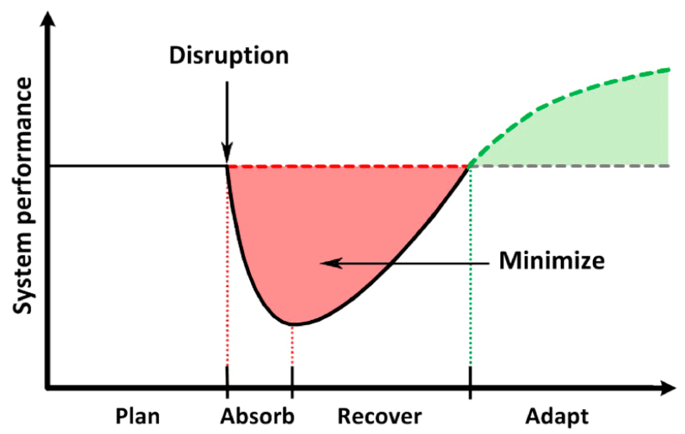
Figure 1. Stages of resilience.
Preprints 68606 g001
The absorption stage is designed to implement unpredictable changes in the basic architecture or behavior of the system, depending on what exactly is subject to destructive influence. Absorption mechanisms can have a multi-layered structure, implementing protection in depth, when the system determines which mechanism should be used if the threat cannot be absorbed at this level. If it is impossible to avoid degradation, then the mechanism of controlled degradation (graceful degradation) is implemented, when the core operations of the system take priority over non-essential services for as long as possible. The system can be pre-configured with an ordered set of less functional states that represent acceptable trade-offs between functionality, performance and cost effectiveness.
The recovery stage includes measures aimed at restoring the lost functionality and performance as quickly and cost efficiently as possible. The adaptation phase focuses on the ability of the system to change to better cope with future threats.
The principles of Affordable Resilience are often used in the design and operation of resilient systems, taking into account resource constraints [26]. Affordable resilience involves achieving an effective balance between the life cycle cost and the technical characteristics of the system’s resilience. When considering the life cycle for Affordable Resilience, it is necessary to take into account not only the risks and challenges associated with known and unknown perturbations in time, but also the opportunities to find gains in known and unknown future environments.
In [26,27] it is proposed to balance cost and the benefits of obtained resilience to achieve Affordable resilience (Figure 2).
After determining the affordable levels of resilience for each key performance indicator, the priorities of these indicators can be determined on the basis of the Multi-attribute Utility Theory [28] or Analytical Hierarchy Process [29]. As a rule, the priorities of performance indicators of the resilient system depend on the applied domain area.
In the papers [30,31], to optimize the parameters and hyperparameters g of the system, taking into account resource constraints, it is proposed to find a trade-off between the performance criterion J under normal conditions and the integral indicator of system resilience R under the influence of disturbances, that is
g * = arg m a x G η J ¯ ( g ) + ( 1 η ) R ( g ) ,
where η is coefficient that regulates the trade-off between the performance criterion and the integral resilience index of the system within the control period.
Researchers and engineers involved in the development of resilient systems have formulated a number of heuristics that should be relied on when designing resilient systems [11,15,18]:
  • functional redundancy or diversity, which consists in the existence of alternative ways to perform a certain function;
  • hardware redundancy, which is the reservation of the hardware to protect against hardware failures;
  • the possibility of self-restructuring in response to external changes;
  • predictability of the automated system behavior to guarantee trust and avoid frequent human intervention;
  • avoiding excessive complexity caused by poor design practices;
  • the ability of the system to function in the most probable and worst-case scenarios of natural and man-made nature;
  • controlled (graceful) degradation, which is the ability of the system to continue to operate under the influence of an unpredictable destructive factor by transitioning to a state of lower functionality or performance;
  • implementation of a mechanism to control and correct the drift of the system to a non-functional state by making appropriate compromises and timely preventive actions;
  • ensuring the transition to a "neutral" state to prevent further damage under the influence of an unknown destructive disturbance until the problem is thoroughly diagnosed;
  • learning and adaptation, i.e. reconfiguration, optimization and development of the system on the basis of new knowledge constantly obtained from the environment;
  • inspectability of the system, which provides for the possibility of necessary human intervention without requiring unreasonable assumptions from it;
  • a human being should be aware of the situation when there is a need for "quick comprehension" of the situation and the formation of creative solutions;
  • implementation of the possibility of replacing or backing up automation by people when there is a change in the context for which automation is not prepared, but there is enough time for human intervention;
  • implementation of the principle of awareness of intentions, when the system and humans should maintain a common model of intentions to support each other when necessary.
Thus, resilience is a system property and is based on certain principles and stages of processing disturbing influences.

2.2. Vulnerabilities and threats of AISs
In general, AIS operate in imperfect conditions and can be exposed to various disturbances. AI-technology has numerous AI-specific vulnerabilities. In addition to AI-specific vulnerabilities, there are physical environment vulnerabilities that can lead to hardware failures in the deployment environment, as well as vulnerabilities related to safety and cybersecurity of information systems.
One of the AI-specific vulnerabilities is the dependence of the efficiency and security of AI on the quantity and quality of training data. An AIS can be highly effective only if the training data is unbiased. However, data collection or model building may be outsourced to an uncontrolled environment for economic reasons or to comply with local data protection laws. Therefore, the obtained result cannot always be trusted. The data collected in another environment (including synthetic data) may not be relevant to the application environment. In addition, AIS can only analyze correlations in data, but cannot distinguish false correlations from true causal relationships. It creates an additional possibility of data poisoning and data quality reduction.
The low interpretability of modern deep neural networks can also be seen as a vulnerability, since attacks on the AIS cannot be detected by analyzing model parameters and program code, but only by incorrect model behavior [32]. Without interpreting the AIS-decisions, it is difficult for even an expert to understand the reason of AIS performance degradation.
Huge Input and State Spaces and Approximate Decision Boundaries can also be considered to be vulnerabilities. It has been shown that due to the high dimensionality of the feature space, it is possible to search in many directions to select imperceptible modifications to the original data samples that mislead the AIS. Also, the high dimensionality of the input feature space facilitates the presence of so-called non-robust features in the data, which improves the transferability of adversarial examples to other AIS [32,33]. In addition, the high dimensionality of State Spaces complicates the process of adapting to rapid changes in the dependencies between inputs and outputs of AIS. It is difficult to simultaneously avoid catastrophic forgetting and ensure high speed of adaptation of a large AIS to changes.
AIS vulnerabilities can be exploited by hackers, terrorists and all kinds of criminals. In addition, employees who face dismissal as a result of their replacement by AIS may try to discredit the effectiveness of AIS. As AIS is increasingly used in military vehicles, these machines can become a target for the opposing side of an armed conflict. In addition, as the AI-technologies evolves, some AISs can be directed to attack other AISs.
AIS have various resource constraints, which can be a source of threats, as sufficient or excessive resources are needed to implement reliable redundancy, self-diagnosis and recovery, as well as optimization (improvement).
The physical environment is also a source of threats. Such influences as EM Interference, Laser Injection, and Heavy-ion radiation can cause damage to the neural network weighs and cause AIS failures [34]. Also, variations in the supply voltage or direct influence on the clock circuit can lead to a glitch in the clock signal. It leads to incorrect results of intermediate and final calculations in the neural network. In addition, the components of the deployment system may be damaged. If software and artificial intelligence algorithms do not take into account the following system faults when designing, this can lead to AIS failures.
The natural environment can also be a source of threats, as it can contain influences that were not taken into account during training and can be perceived as noise or novelty in the data. The high variability of the observed environment and limited resources for training data collection leads to insufficient generalization. In addition, the environment, in general, is not stationary, and the patterns of the observed process can change unpredictably. As a result, at certain times, the model of mapping inputs to outputs may become irrelevant. A compromised network, infected AIS software and remote access to AIS can be a source of threat to AIS in terms of the ability to acquire its data, structure and parameters, which facilitates the formation of attacks.
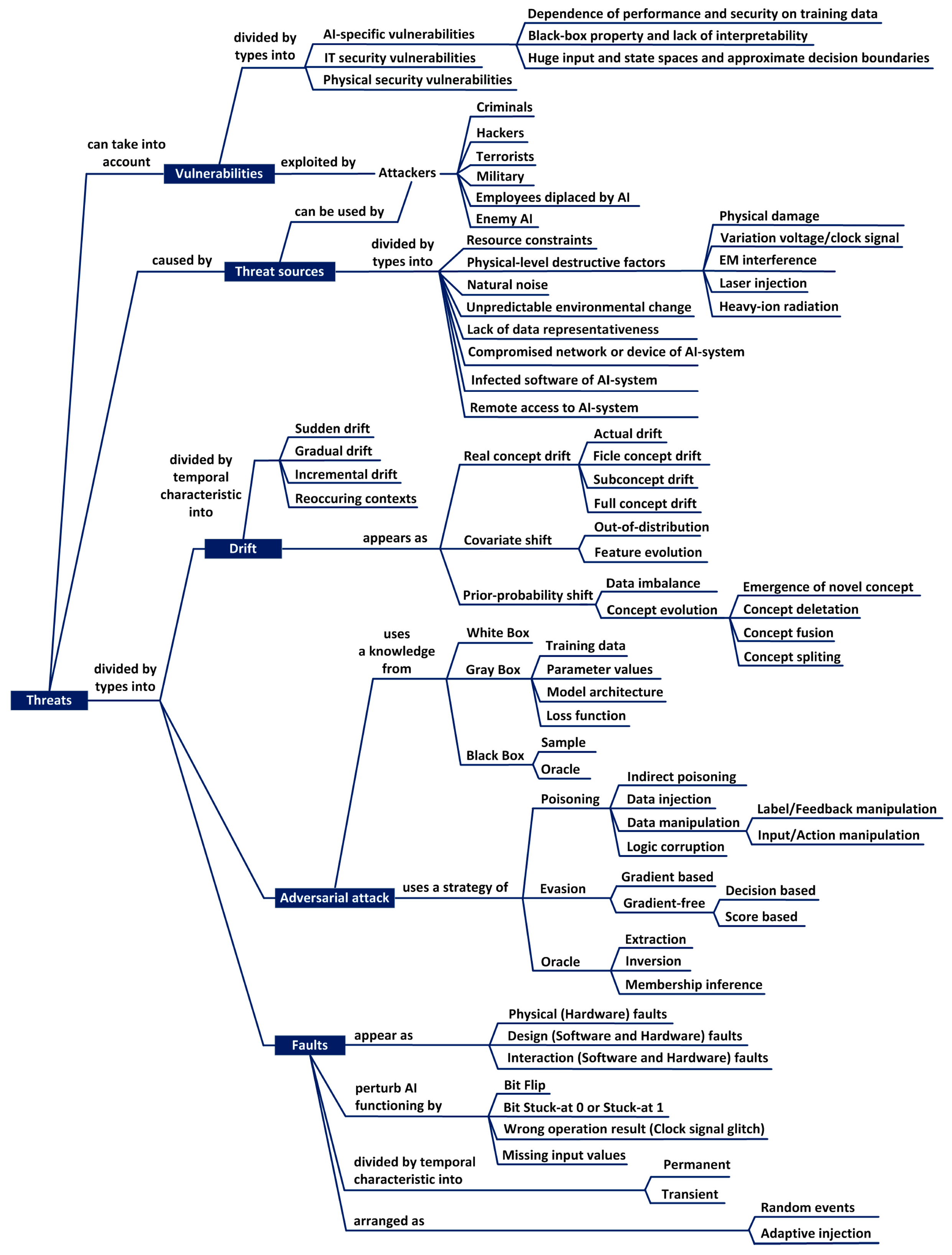
Among AIS threats, there are three main types of disturbances: drift, adversarial attacks, and faults. Each of these types has subtypes depending on their way of formation and specifics of impact.
The drift problem occurs when at a certain time point the test data begins to differ significantly from the training data in certain characteristics, which indicates the need to update the model to avoid performance degradation. Drift in machine learning is divided into real concept drift, covariance shift, and a priori probability shift.
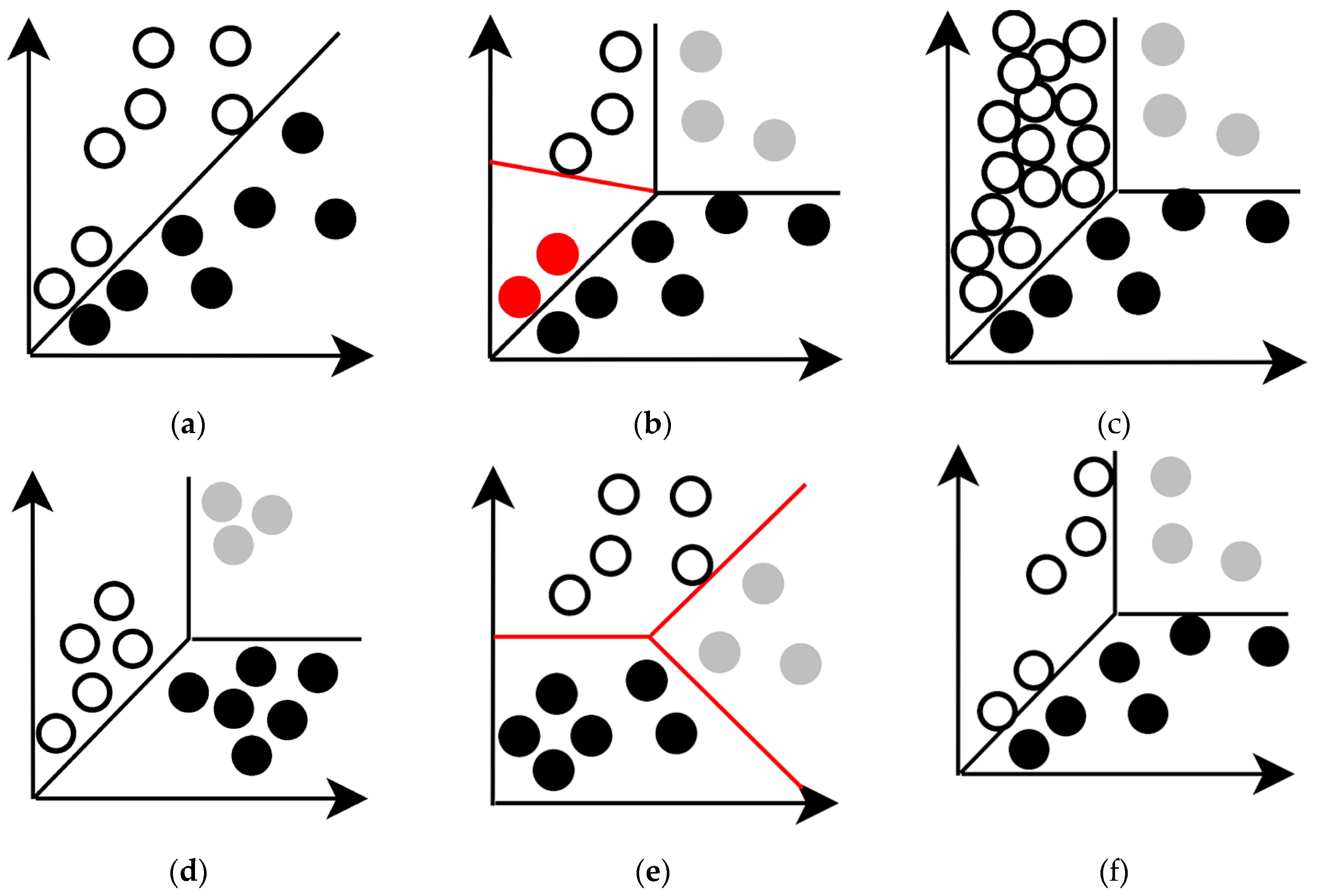
Real concept drift means a change in the distribution of a posteriori probability P t + w ( y | X ) at time t + w compared to the a posteriori probability distribution P t ( y | X ) at time t , which is connected with principal change in the underlying target concept, that is P t ( y | X ) P t + w ( y | X ) , where X is a set of input variables, and y is target variable (Figure 3b). In the case of reinforcement learning, the real drift of concepts occurs as a result of environment context changes (environment shift). In other words, the agent functions under conditions of non-stationary rewards and/or non-stationary transition probabilities between system states [35]. Ficle concept drift, which is a subcategory of real drift and occurs when some data samples belong to two different concepts or contexts at two different times, is considered separately. Subconcept drift or Intersect concept drift is also a subcategory of real drift and occurs when only a subset of the dataset changes its target variable or rewards feedback after drift has occurred. Full concept drift or Severe concept drift is a subcategory of real concept drift, which occurs when target variables of all data points change after the drift occurs. In the case of reinforcement learning, Full concept drift can be associated with changes in action-reward feedback and transition probabilities for all historical state-action pairs.
Covariate shift, or virtual concept drift as it is commonly called in the literature, occurs when input data distribution changes without affecting the target concept (Figure 3c). In mathematical terms, P t y x = P t + w ( y | x ) and P t ( x ) P t + w ( x ) . Although in practice, changes in the data and the posterior probability distributions often happen simultaneously. So, covariate shift can be a component of overall drift or the initial stage of real concept drift. Out-of-distribution data can be considered one of the subcategories of Covariate shift. Out-of-distribution data may have an element of novelty and it do not ensure the reliability of the analysis. This may be related to the lack of training data in appropriate region of space, which increases epistemic uncertainty. Or it may be caused by the fact that the data is completely outside the training distribution and the model could not extrapolate effectively. It is a case of aleatoric uncertainty. Another subcategory Covariate shift is related to dynamically arising new attributes in the input space. This subcategory is also called Feature-evolution. Mathematically, this can be described as X t X t + w and as a result P t ( x ) P t + w ( x ) . This can occur if the AIS is evolving and new data sources are added. When AIS in inference mode encounters data that falls outside the distribution on which it was trained, AIS reaction can be unpredictable and have catastrophic consequences. Prior-probability shift is another type of drift and is associated with the appearance of data imbalance or a change in the set of concepts or contexts. In the case of data classification, prior-probability shift means that there is a change in probabilities P ( y ) due to unbalanced class samples (Figure 3d), emergence of novel classes (Figure 3e), removal of existing classes (Concept deletion), concept fusion (Figure 3f) or splitting certain classes into several subclasses (Concept splitting).
Figure 3. Visual illustration of different types of concept drift for three-class classifier: a—original data distribution and decision boundary of classifier; b—real concept drift; c—virtual concept drift; d—imbalance of classes; e—the emergence of a new class; f—class merging.
Preprints 68606 g003
In terms of the time characteristics of concept drift, they can be classified into abrupt (sudden), gradual, incremental, re-occurring and blip [36]. Abrupt concept drift is the rapid change of an old concept to a new one. In this case, the performance of the model suddenly decreases, and there is a need to quickly train a new concept to restore performance. Gradual drift has an overlapping concept, and after some period of time, the new concept becomes stable. In incremental concept drift, certain concept vanished from the observations at certain time and never occurred again. In a recurring type of drift, a concept reappears after a long period of time. А recurring change of concept occurs in the flow. Such drift can have cyclic and acyclic behavior. Cyclical drift occurs when there are seasonal fluctuations. For example, sales of cold clothes increase during the summer season. An acyclic phenomenon is observed when the price of electricity increases due to an increase in the price of gasoline and normally it returns to the previous price. A blip drift is a very rapid change in a concept or a rare event, so it is considered as an outlier in a stationary distribution. In other words, in general, blip drift is usually not even considered to be concept drift.
Significant destructive effects on AIS can be caused by various faults. Faults in a computer system can cause errors. An error is such manifestations of faults that leads to a deviation of the actual state of a system element from the expected one [34]. If a fault does not cause an error, then such a fault is called a sleeping fault. As a result of errors, failures can occur, meaning that the system is unable to perform its intended functionality or behavior. In general, faults can be divided into four groups:
  • physical faults that lead to persistent failures or short-term failures of AIS hardware;
  • design faults, which are the result of erroneous actions made during the creation of AIS and lead to the appearance of defects in both hardware and software;
  • interaction faults that result from the impact of external factors on AIS hardware and software;
  • software faults caused by the effect of software aging, which lead to persistent failures or short-term failure of AIS software.
Failures of the system and its components can be caused by a single fault, a group of faults, or a sequential manifestation of faults in the form of a "pathological" chain.
Figure 4 illustrates the causal relationship between a hardware fault, error, and failure. A failure causes a violation of the predictable behavior of a neural network that is deployed to perform its task in a computing environment.
Hardware faults can be classified according to their time characteristics (Figure 5) [37]:
  • permanent fault which is continuous and stable over time as result of physical damage;
  • transient fault which can only persist for a short period of time as result of external disturbances.
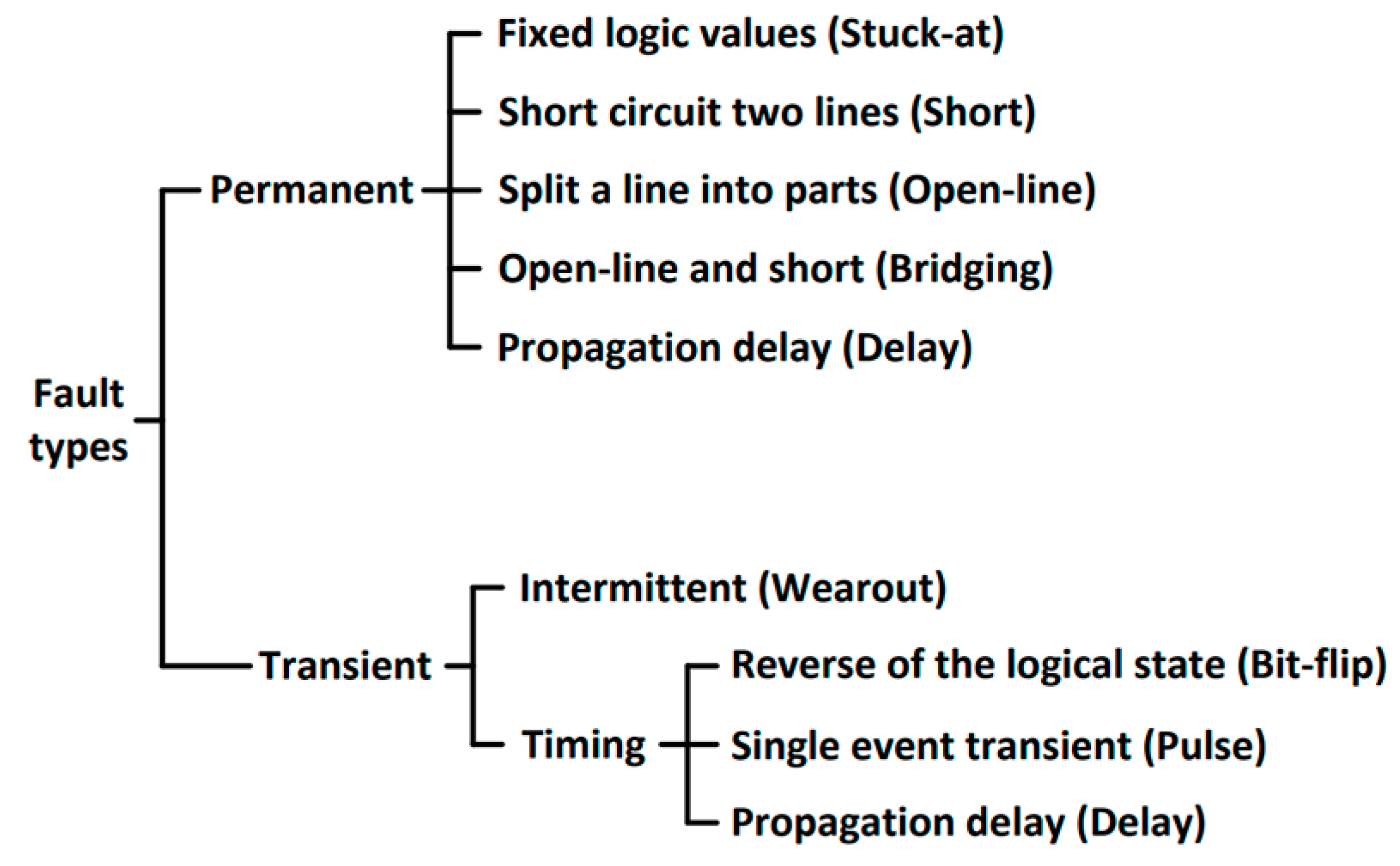
Figure 5. Types of hardware faults in the computing environment.
Preprints 68606 g005
Permanent fault types can simulate many defects in transistors and interconnect structures at the logic level with a fairly high accuracy The most common model of permanent defects is the so-called "stuck-at", which consists in maintaining an exclusively high (stuck-at-1) or low (stuck-at-0) state on data or control lines. Also, to assess fault tolerance in computing systems, researchers necessarily consider faults such as "stuck-open" or "stuck-short" state [34]. Faults of this type allow us to describe cases when a "floating" line has a high capacity and retains its charge for a considerable time in modern semiconductor technologies.
Transient faults cover the vast majority of faults that occur in digital computing systems built on modern semiconductor technology. Future technologies are expected to be even more susceptible to transient faults due to greater sensitivity to environmental influences and high material stresses in highly miniaturized media. Transient faults that recur at a certain frequency are usually caused by extreme or unstable device operation and are more difficult to detect than permanent faults. Transient faults are associated with the impact on the parameters of circuits that determine the time characteristics, rather than on the structure of circuits. Transient faults include an unpredictable delay in signal propagation, random bit switching in memory registers, impulsive changes in logic circuits [37].
There are several physical methods of injecting faults with malicious intent. In practice, fault injection is realized due to a system clock failure, that is, circuit synchronization, power sag to a certain level, electromagnetic effects on semiconductors, irradiation with heavy ions, laser beam effects on memory, and software rowhammer attacks on memory bits [2].
Laser beam can inject an error into static random access memory (SRAM). When a laser beam is applied to silicon, a temporary conductive channel is formed in the dielectric, which causes the transistor to switch states in a precise and controlled manner [38]. By carefully adjusting the parameters of the laser beam, such as its diameter, emitted energy, and impact coordinate, an attacker can accurately change any bit in the SRAM memory. The laser beam has been widely and successfully used in conjunction with differential fault analysis to extract the private key of encryption chips.
Rowhammer-attacks can cause errors in DRAM memory. This type of attack takes advantage of the electrical interaction between neighboring memory cells [39]. By quickly and repeatedly accessing a certain region of physical memory, the bit in the neighboring region can be inverted. By profiling bit inverting patterns in the DRAM module and abusing memory management functions, a row hammer can reliably invert a single bit at any address in the software stack. There are known examples of using the Rowhammer attack to break memory isolation in virtualized systems and to obtain root rights in the Android system.
Laser beam and Rowhammer attacks can inject errors into memory with extremely high accuracy. However, to inject multiple errors, the laser beam must be reconfigured, and a Rowhammer attack requires moving target data into memory. Reconfiguring the laser beam, as well as moving data, requires certain overhead. Therefore, the design of neural network algorithms should provide resistance to a certain level of inverted bits to make these attacks unusable from a practical point of view.
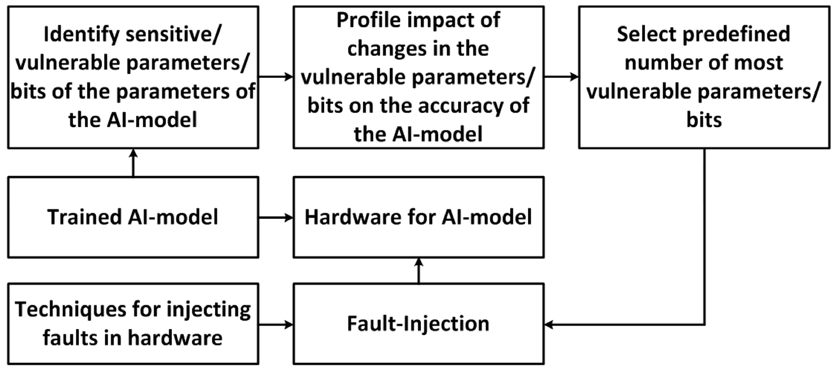
The injection of faults and errors into the digital system for deploying AI can be carried out in an adaptive manner, taking into account feedback (Figure 6). In this case, attack success is monitored at the output of the neural network. At the same time, Single Bias Attack (SBA) or Gradient Descent Attack (GDA) can be used to adaptively influence on the system [2].
The output of neural networks is highly dependent on the biases in the output layer, so SBA is implemented by increasing only one value of the bias of the neuron associated with the target category. SBA is designed for cases where hiddenness of the attack is not required. For cases where hiddenness is important, GDA is used, where gradient descent searches for a set of parameters that need to be changed for the attack success. The authors of [2,38] proposed to apply Alternating Direction Method of Multipliers (ADMM) to optimize the attack while ensuring that the data analysis other than the ones specified is unaffected and the modification in the parameters is minimum.
The importance of protecting against adaptive fault and error injection algorithms is related to the trend of moving real-time intelligent computing to edge devices. These devices are more likely to be physically accessible to an attacker, which increases the possibility of misleading devices. Modern cyber-physical systems and the Internet of Things are typical platforms for deployement of intelligent algorithms that require protection against fault injection.
An equally harmful destructive factor for machine learning systems is data corruption, missing values, and errors in training and test data. Missing values in features lead to loss of information, and errors in target data labels lead to misinformation and reduced learning efficiency. Missing values in data are often caused by software or hardware faults related to data collection, transmission, and storage.
Researchers have found that neural network algorithms are sensitive to so-called adversarial attacks, which involve manipulating data or a model to reduce the effectiveness of AIS [2]. It was noted that adversarial attacks have the following properties:
  • imperceptibility, which consists in the existence of ways of such minimal (not visible to humans) modification of data that leads to inadequate functioning of AI;
  • the possibility of Targeted Manipulation on the output of the neural network to manipulate the system for your own benefit and gain;
  • transferability of adversarial examples obtained for one model in order to apply them to another model if the models perform a common task, which allows attackers to use a surrogate model (oracle) to generate attacks for the target model;
  • the lack of generally accepted theoretical models to explain the effectiveness of adversarial attacks, making any of the developed defense mechanisms not universal.
Machine learning model, deployment environment, and data generation source can be the target of attacks. Attacks can be divided into three main types according to the purpose:
  • availability attacks, which leads to the inability of the end user to use the AIS;
  • integrity attacks, which leads to incorrect AIS decisions;
  • confidentiality attacks, where the attacker's goal is to intercept communication between two parties and obtain private information.
According to strategy, adversarial attacks can be classified into: evasion attacks, poisoning attacks, and oracle attacks [40].
Evasion is an attack on AI under inference by looking for modification of input sample to confuse the machine learning model. The main component of a adversarial attack is a adversarial data sample x ' with a small perturbation (adding a noise component) x ' = x + ε , which leads to a significant change in the output of the network, described by the function f ( x ) , thus f ( x ' ) f ( x ) . The neural network weights θ are treated as fixed and only the input test sample x is subject to optimization in order to generate the adversarial sample x ' = x + ε . This attack involves an optimization process of finding a small perturbation ε that will cause a wrong AIS decision. Evasion attacks are divided into gradient-based evasion and gradient-free evasion. Gradient-based evasion uses one-step or iterative gradient optimization algorithms with imperceptibility constraints to improve the effectiveness of these attacks. The most well-known gradient-based attacks are Fast Gradient Sign Method (FGSM), iterative-FGSM (iFGSM), Jacobian Saliency Map Attack (JSMA), Carlini and Wagner (C&W) attack and training dataset unaware attack (TrISec) [41].
Gradient-free evasion attacks are divided into Score-based Evasion Attacks and Decision-based Evasion Attacks. Score-based Evasion Attacks uses output scores/probabilities to predict the direction and strength of the next manipulation of the input data. Decision-based Evasion Attacks start by generating stronger input noise that causes incorrect model decisions, and then the noise is iteratively reduced until it becomes undetectable. The goal of Decision-based Evasion Attacks is to explore different parts of the decision boundary and find the minimum amount of noise that misleads the model. However, the cost of these attacks in terms of the number of requests is very high. Therefore, FaDec attacks use adaptive step sizes to reduce the computational cost of Decision-based Evasion Attacks to achieve the smallest perturbation with the minimal number of iterations [42].
Poisoning attacks involve corrupting the data or logic of a model to degrade the learning outcome [43]. In this case, poisoning data before it is pre-processed is considered as indirect poisoning. Direct poisoning refers to the data injection or data manipulation, or model modification by means of logical corruption. The injection of adversarial data leads to a change in the distribution and a shift in the decision boundary based on linear programming or gradient ascent methods. Data manipulation can consist of modifying or replacing labels, feedback or input data. Logic Corruption is the intrusion into a machine learning algorithm to change the learning process or model in an adverse way.
An oracle attack involves an attacker using access to the software interface to create a surrogate model that retains a significant portion of the original model's functionality. Surrogate model provide efficient way to find an evasion attack which is transferred to the original model. Oracle attacks are divided into: extraction attacks, inversion attacks, and membership inference [44]. The goal of the extraction attack is to extract the architectural details of the model from the observations of the original predictions and class probabilities. Inversion attacks are an attempt to recover training data. Membership inference attack allows the adversary to identify specific data points from the distribution of the training dataset.
The attacks can be categorized according to our knowledge of the data analysis model on:
  • white-box attacks, which are formed on the basis of full knowledge of the data, model and training algorithm, used by AIS developers to augment data or evaluate model robustness;
  • gray-box attacks based on the use of partial information (Model Architecture, Parameter Values, Loss Function or Training Data), but sufficient to attack on the AIS;
  • black-box attacks that are formed by accessing the interface of a real AI-model or oracle to send data and receive a response.
Various methods of creating a surrogate model, gradient estimation methods, and various heuristic algorithms are used to form adversarial black box attacks. This type of attack poses the greatest threat in practice.
Figure 7 shows the ontological diagram of AIS threats as summarization the above review.
Figure 7. Ontological diagram of AIS threats.
Preprints 68606 g007
Thus, all of the following can be considered AIS disturbances: fault injection, adversarial attacks and concept drift, including novelty (out-of- distribution), missing values, and data errors. There are many types and subtypes of AIS disturbance. The research of each disturbance type is still a relevant area of research, especially where the research of the complex impact of different types of disturbances is concerned.

2.3. Taxonomy and ontology of AIS resilience

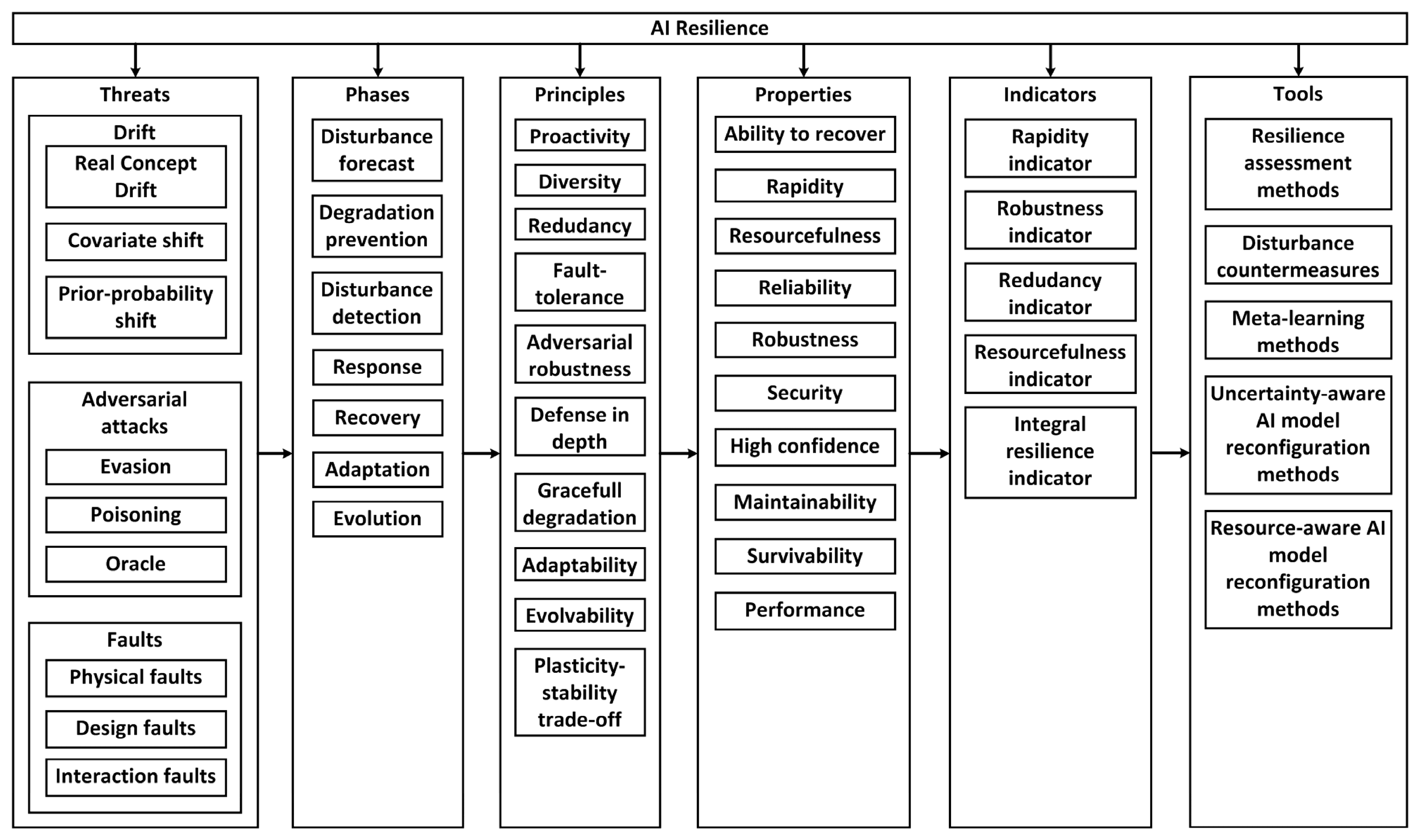
The main elements of the taxonomic diagram of AIS resilience are: threats (drift, faults and adversarial attacks); phases (plan, absorb, recover, adapt) of AIS operational cycle; principles on which the AIS resilience is based; properties that characterize resilient AIS; indicators that can be used to assess AIS resilience; tools for ensuring AIS resilience (Figure 8).
Certain resilience phases (stages) can be split and detailed. Based on the analysis of [11,12], the following phases of the operating cycle of resilient AIS should be implemented: disturbance forecast, degradation prevention, disturbance detection, response, recovery, adаptation and evolution. Disturbance Forecast is a proactive mechanism that provides knowledge about early symptoms of disturbance and readiness to a certain type of known disturbance.
Degradation prevention is the application of available solutions and knowledge about the disturbing factor to absorb the disturbance (ensure robustness) in order to minimize the impact of the disturbance on the AIS performance. Not every disturbance can be completely absorbed, but in order to produce an optimal AIS response, the disturbance should be detected and identified by its type. The purpose of disturbance detection is to optimally reallocate resources or prioritize certain decisions in the face of inevitable performance degradation. Moreover, an important stage of resilient AIS is the restoration of the initial performance and adaptation to the impact of disturbances. The last phase of the operational cycle involves searching for and implementing opportunities for evolutionary changes that ensure the best fit of the system architecture and parameters to new conditions and tasks.
The implementation of resilient AIS is based on the general principles of designing resilient systems with taking into account the specifics of modern neural network technologies. The systematization of papers [11,16] allows formulating the following principles of ensuring the AIS resilience: proactivity, diversity, redudancy, fault-tolerance, adversarial robustness, defense in depth, gracefull degradation, adaptability, plasticity-stability trade-off and evaluability.
The principle of diversity implies the inclusion of randomization and multi-versioning into implementation of system components [15]. Different versions of the components can implement different architectures, subsamples and subspaces of features or data modalities, use different data augmentations, and different initializations of neural network weights. In this case, the use of the voting method for the diverse components of the AIS helps to reduce the variance of the complex AI-model in the inference mode. Diversity causes the redundancy of AIS and additional development overhead, but on the other hand it complicates the attack and mitigates any disturbing influence.
The principles of Fault-tolerance and Adversarial robustness provide for absorption of faults and adversarial attacks on AIS by using special architectural solutions and training methods. The Defense in Depth principle suggests combining several mechanisms of AIS defense, which consistently counteract the destructive impact. If one mechanism fails to provide defense, another is activated to prevent destructive effects.
The principle of gracefull degradation is the pre-configuration of the AIS with a set of progressively less functional states that represent acceptable trade-offs between functionality and safety. The transition to a less functional state can be smooth, providing a gradual decrease in performance without complete breakdown of the AIS. Concepts such as granularity of predictions and model hierarchy, zero-shot learning, and decision rejection are common ways to allow AIS to handle unexpected events while continuing to provide at least a minimum acceptable level of service.
The principles of Adaptability, Evaluability, and Plasticity-stability trade-off are interrelated and specify the ability of AIS to learn and, more specifically, engage in continual learning with regularization to avoid the effect of overfitting and catastrophic forgetting [4,6,14]. The principle of AIS Evaluability implies the possibility of making necessary structural, architectural or other changes to the AIS, which will reduce vulnerability and increase resilience to potential future destructive impacts. These principles also include improving the speed of adaptation to new disturbances through meta-learning techniques.
A resilient AIS can be characterized by a set of properties: ability to recover, rapidity, resourcefulness, reliability, robustness, security, high confidence, maintainability, survivability, performance. These properties should be self explanatory from their names or from description in the previous subsections. A set of indicator (metrics) can be proposed to AIS resilience assess : rapidity indicator, robustness indicator, redundancy indicator, resourcefulness indicator, integral resilience indicator. Integral resilience indicator deserves special attention, as it simultaneously takes into account the degree of robustness and recovery rate. Resourcefulness can be conceptualized as consisting of the ability to apply resources to meet established priorities and achieve goals [11]. An organizational resourcefulness can be measured by ratio of the increase in resilience to the increase in the amount of involved resources [11,45].
A certain set of tools should be used to ensure AIS resilience. The most important tools are resilience assessment methods, which allow to assess, compare and optimize the AIS resilience. To ensure robustness and peformance recovery, it is necessary to use various disturbance countermeasures. Meta-learning tools, methods of reconfiguring the AI model with regard to performance or resources privide certain level of evolvability. The implementation of AIS adaptation and evolution mechanisms requires the inclusion of constraints imposed by the principle of plasticity-stability trade-off [6,14].
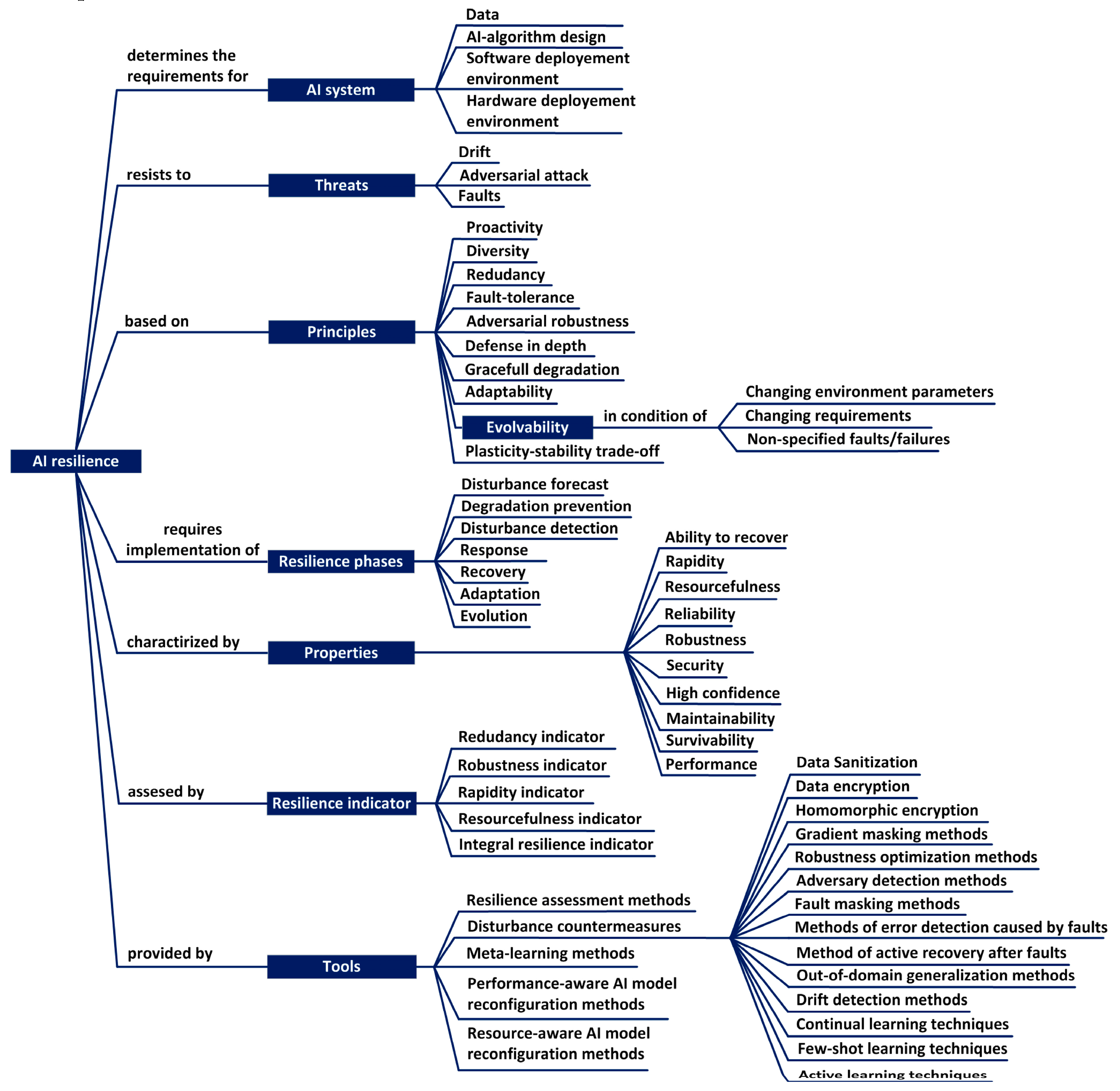
Figure 9 shows an ontological diagram of the AIS resilience. Moreover, the diagram specifies the conditions for the emergence of the AIS evolution. AIS should be improved to quickly eliminate drift caused by these changes through domain adaptation and meta-learning. In addition, there is a need to initiate evolutionary improvement of the AIS as a response to influence of non-specified faults/failures, the effective processing of which was not provided in the current configuration.
In addition, Figure 9 shows a list of the main disturbance countermeasures required for absorbing disturbances, graceful degradation and peformance recovery. This list includes the following countermeasures: data sanitization, data encryption, homomorphic encryption; gradient masking methods; robustness optimization methods, adversary detection methods, fault masking methods, methods of error detection caused by faults, method of active recovery after faults, drift detection methods, continual learning techniques, few-shot learning techniques, active learning techniques [46,47,48].
Data sanitization and data encryption methods prevent data poisoning. Data Sanitization methods are based on the Reject on Negative Impact approach; they remove samples from the dataset which negatively affect the performance of the AIS [33,47]. Homomorphic Encryption methods provide defense against cyber attacks on privacy. Homomorphic Encryption encrypts data in a form that a neural network can process without decrypting the data. An encryption scheme is homomorphic for operation ∗; without the access to the secret key, the following holds [33]:
Enc(x1) * Enc(x2) = Enc(x1 * x2),
where Enc(·) denotes the encryption function.
Gradient masking methods, Robustness optimization methods, and Adversary detection methods are used to defend the AIS against adversarial attacks in the inference mode. Fault masking methods, Methods of error detection caused by faults and Method of active recovery after faults are used to mitigate the effect of faults on AIS performance [34,49]. Drift detection methods, Continuous learning techniques, Few-shot learning techniques, and Active learning techniques are used for the effective functioning of AI under drift conditions [4,5,6].

3. Models and methods to ensure and assess AI resilience

3.1. Proactivity and robustness

The proactivity of the AIS implies preparation for absorbing disturbances of a known type and predicting the beginning of the impact of known and unknown disturbances on the AIS performance. The ability of the AIS to absorb disturbances is related to the robustness of AIS models. The choice of the method for absorbing and recognizing (detecting) a disturbance depends on the type of disturbance.
Table 1 presents the approaches and their corresponding methods and algorithms aimed at resistance to adversarial attacks. The first approach is Gradient masking, the simplest implementations of which are methods of special data preprocessing, such as jpeg compression, random padding and resizing [50,51] defensive distillation [52], randomly choosing a model from a set of models or using dropout [53], the use of generative models [54,55], and discrete atomic compression [56]. The second approach is to optimize the robustness at the preparatory stage of the resilient system's operating cycle. The most general and simplest method of optimizing robustness involves training on generated perturbed training samples combined with certain regularization methods [57,58,59]. These methods minimize the impact of small perturbations on the input data based on Jacobian regularization or L2-distance between feature representations for original and perturbed samples. Sparse coding-based methods of feature representation are also considered to be a method of optimizing robustness due to the low-pass filtering effect [60]. The latest approach is to detect adversarial evasion attacks in the test data and poisoning attacks in the training data [61,62,63]. However, Carlini and Wagner rigorously demonstrate that the properties of adversarial samples are difficult and resource-intensive to detect [64].
The analysis of Table 1 shows that, with enough computing resources, the most promising approach is based on robustness optimization. In addition, this approach is compatible with the use of other approaches, allowing to implement the principle of defense in depth.
Table 2 shows the approaches which are used to ensure robustness to the injection of faults in the computing environment where neural networks are deployed: fault masking [68,69,70], the introduction of explicit redundancy [71,72,73] and error detection [74,75,76]. Faults are understood as accidental or intentional bit flips in memory, which store the weights or the output value of the neuron.
Fault masking can be implemented in the form of architectural solutions that automatically correct or eliminate the impact of a small portion of neural weights’ faults. Optimizing the architecture to increase robustness means minimizing the maximum error at the output of the neural network for a given number of bit-flips in neural weights or results of neural intermediate calculations. However, architecture optimization is traditionally a very resource-intensive process. A similar effect can be achieved by redistributing the knowledge among multiple neurons and weights, reducing the importance of individual neurons. This redistribution can be performed by including a regularization (penalty) term in the loss function to indirectly incorporate faults in conventional algorithms. Redundancy methods have traditionally been used in reliability theory to ensure fault tolerance. Similarly, duplication of critical neurons and synapses and model ensembles are used in neural networks. Error detection is another approach to fault handling which provides Rejection Option in the presence of neural weight errors caused by faults. In [75,77], sum checking and low-collision hash function are proposed in order to detect changes in the neural network weight under the influence of memory faults. In the paper [76], the current value of the contrastive loss function for the diagnostic data is compared with a reference value for fault detection. The reference value is calculated as contrastive loss value on the test diagnostic data samples under normal conditions.
Table 3 shows the approaches used to detect and mitigate [concept] drift. Out-of-domain generalization and Ensemble selection are two main approaches for absorbing small concept drifts. Out-of-domain generalization can be achieved by using domain randomization [78] and adversarial domain augmentation [79], building Domain-invariant representation [80] or Heterogeneous-domain knowledge propagation [81]. In [78,79], domain randomization and adversarial domain augmentation, which increase the robustness of the model under bounded data distribution shifts, are proposed. Domain randomization is the generation of synthetic data with large enough variations so that that real-world data are simply viewed as another domain variation [78]. Adversarial domain augmentation creates multiple augmented domains from the source domain by leveraging adversarial training with relaxed domain discrepancy constraint based on the Wasserstein auto-encoder [79]. Transfer learning and multi-task or multiple-source domain learning also reinforce resistance to out-of-distribution perturbations [80,81]. Ensemble algorithms can also be quite useful for mitigating the effects of drift. For example, Dynamically weighted Ensemble [82] adjusts the weight of individual elements of the ensemble depending on their relevance to the input data. The feature dropping algorithm [83] uses each element of the ensemble to correspond to a separate feature and can be excluded from the voting procedure if drift is observed on this particular element of the ensemble.
In order to handle concept drift in a timely manner, tools to detect it are necessary. Data distribution-based detectors estimate the similarity between the data distributions in two different time-windows [84]. These algorithms consider the distribution of data points, but changes in the data distributions do not always affect the predictor performance. Performance-based approaches trace deviations in the online learner’s output error to detect changes [85]. The main advantage of performance-based approaches is that they only handle the change when the performance is affected. However, the main challenge is that these methods require a quick arrival of feedback on the predictions, which is not always available. Multiple hypothesis-based drift detectors are hybrid approaches that apply several detection methods and aggregate their results in parallel or hierarchically [86]. The first layer is the warning layer to alert the system about a potential occurrence of concept drift. The second layer is the validation layer that confirms or rejects the warning signaled from the first layer. Context-based detectors use context information available from the AIS and data to detect the drift. For example, [87] used model explanation methodologies to interpret, visualize and detect concept drift. In [88], authors designed a concept drift detector using historical drift trends to calculate the probability of expecting a drift using online and predictive approaches.
In practice, AIS is often uncertain due to a lack of knowledge. In order to correctly handle such situations, Out-of-distribution data detection algorithms should be used. Methods for implementing Out-of-distribution data detection can be divided into three groups : methods based on data and training; methods based on AI model; methods based on post-hoc processing.
Methods based on data and training are aimed at obtaining representations which can produce accurate uncertainty evaluation where necessary [89]. In this category of methods the uncertainties are calibrated using additional data. Additional data can be generated by a generative model, or obtained by perturbing the original data with adversarial attacks, or taken from a separate additional dataset.
In model-based methodsthe uncertainty evaluator is built into the architecture of the model. Such approaches can take distributions over the model parameters [90]. The uncertainty between the training and test distribution are considered to arise from uncertainties in the model itself. Model-based methods rely on probablistic forward pass, allowing the weight uncertainties to propagate through the network and giving a probability distribution for the output. These methods can be used with bayesian neural networks and a hypernetwork which generate the weights for a target neural network. The key advantage of hypernetwork is its flexibility and scalability. Some model-based methods might leverage gradients, ensembles, artefacts of dynamic and stochastic training processes, earlier snapshots of the network and other information to evaluate uncertainty.
Post-hoc methods focus on the output of the model and use it to calibrate the predictive uncertainty [91]. Post-hoc methods provide a more accurate reflection of the prediction confidence based on transformation of AIS-output. It can be implemented by a simple temperature scaling or by more complicated means. For example, [92] introduces an auxiliary class which identifies miss-classified samples and explicitly calibrates AI-model on out-of-distribution datasets. Post-hoc methods can be incorporated with any AI architecture and, arguably, any AI model.
The analysis of Table 3 shows that it is possible to increase robustness to covariate shift by Out-of-domain generalization and reduce the impact of a certain level of concept drift in the case of a moderately sized models without high dimensionality of the feature space. Сoncept drift detection is not reliable enough when exposed to noise, adversarial attacks or faults. Whilst there are methods to ensure Out-of-distribution data detection, they are usually computationally expensive.

3.2. Graceful degradation

Adversarial attacks, fault injections, concept drifts, and out-of-distribution examples cannot always be absorbed, so the development of graceful degradation remains relevant [2,6]. Table 4 summarizes the three most well-known approaches to ensuring graceful degradation of AIS : implementing prediction granularity, Zero-Shot Learning and Switching between models or branches.
Prediction granularity consists in the implementation of hierarchical decision-making [93,94]. If the prediction at the lowest hierarchical level is not sufficiently confident, then the AIS should favor a highly confident prediction at a higher hierarchical level. In this case, the response design should be provided for processing high-level coarse-grained prediction. In [93], a hierarchical classification is proposed, where superclasses are predicted on lower layers of the neural network, and fine-grained predictions are on high-level layers of the neural network. In [94], a hierarchical image classification combined with multi-resolution recognition is proposed to simplify the task of recognizing more abstract classes that are recognized on images with lower resolution.
Table 4. Approaches and algorithms to ensure the graceful degradation.
Approach Capability Weakness Methods and Algorithms
Prediction granularity (hierarchical prediction) Using confident coarse-grained prediction instead of low-confident fine-grained prediction Approach efficiency depends on architectural solution, data balanciness for each hierarchical level and response design for coarse-grained prediction. Nested Learning for Multi-Level Classification [93].
Coarse-to-Fine Grained Classification [94].
Generalized
Zero-Shot Learning
Ability to recognize samples whose categories may not have been seen at training Not reliable enough due to hubness in semantic space and projection domain shift problem. Embedding-based methods [95].
Generative-based methods [96].
Switching between models or branches Cost or performance aware
adaptive inference
Complicated training and inference protocols. Switching between simpler and complex model [97].
Adaptive inference with Self-Knowledge Distillation [98].
Adaptive inference with Early-Exit Networks [99].
Zero-shot learning aims to build AI-models which can classify objects of unseen classes (target domain) via transferring knowledge obtained from other seen classes (source domain) with the help of semantic information. Semantic information bridges the gap between the seen and unseen classes by embedding the names of both seen and unseen classes in high-dimensional vectors from a shared embedding space. Pragmatic version of Zero-Shot learning recognizes samples from both seen and unseen classes [95]. This version of Zero-Shot learning is called Generalized Zero-Shot learning. Generalized Zero-Shot learning methods can be broadly categorized into Embedding-based methods and Generative-based methods. Embedding-based methods involve learning an embedding space to associate the low-level features of seen classes with their corresponding semantic vectors [95]. The learned projection function is used to recognize novel classes by measuring the similarity score between the prototype representations and predicted representations of the data samples in the embedding space. Out-of-distribution detector is needed to separate the seen class instances from those of the unseen classes. Generative-based methods involve training a model to generate examples or features for the unseen classes based on the samples of seen classes and semantic representations of both classes. Generated samples for unseen classes can be used by conventional supervised learning to update the AI-model.
In addition, Zero-shot learning has spread beyond classification tasks to regression and reinforcement learning tasks. Unlike current reinforcement learning agents, a zero-shot reinforcement learning agent should solve any reinforcement learning task in a given environment, instantly with no additional planning or learning [100]. This means a shift from the reward-centric reinforcement learning paradigm towards "controllable" agents. Agent can follow arbitrary instructions in an environment. In [101], a Zero-Shot learning method was proposed for the regression problem that learns models from features and aggregates them using side information. Moreover, the aggregation procedure was improved by learning the correspondence between side information and feature-induced models.
Zero-shot learning techniques often lack reliable confidence estimates and as such will not be applicable to AIS where high error rates are not permitted. However, one way to improve the reliability of AIS under epistemic uncertainty is to combine Zero-shot learning with Prediction granularity [102].
Another approach to graceful degradation is adaptive inference, which switches between models or branches with different complexity depending on the confidence of the decisions or the impact of disturbances. For example, in [97] it was proposed switching to the simpler model if sudden concept drifts occurs and switching back to the complex model for typical situations. A simpler model better absorbs sudden conceptual shifts and adapts to them faster, although in general it is less accurate. In [99], Early-Exit Networks were proposed to tailor the computational depth of each input sample at runtime. Proposed approach allows resources (time) to be saved when processing simple samples under normal conditions and increases computational resource allocation to improve the reliability of decisions when exposed to perturbations or hard data examples. In [98], improvements to this approach were proposed by introducing the Self-Knowledge Distillation mechanism and multi-granularity of the prediction.

3.3. Adaptation and evolution

The process of recovery and improvement of AI performance in a changing environment or tasks is associated with the implementation of reactive mechanisms of adaptation and evolution. Three main approaches are used to ensure the recovery and improvement of AIS throughout the life cycle: Active / continual/lifelong learning; Domain Adaptation; Meta-learning (Table 5).
In active learning, the goal of the algorithm is to select the data point that causes uncertainty and will be most appropriate for improving the performance of the AI model. A special aspect of active learning is a limited data annotation budget. The data can come in a stream from which data points need to be selected for labeling [103]. Unlabeled data can be stored in a pool from which samples are iteratively selected for labeling and training until the algorithm's performance stops increasing [104]. If annotation of data is not expensive and obtaining the annotation is not a problem, then a continual learning strategy is more appropriate. The main problem of continual learning is the need to combat catastrophic forgetting based on regularizations which impose constraints on the weight updates [105], memorable examples in the data space [106] and change the architecture of the model to handle new information [107].
In domain adaptation the goal is to create a system trained on one distribution, but operating in the context of another distribution. Domain adaptation methods can be split into Discrepancy-based Domain Adaptation, Adversarial Domain Adaptation, Reconstruction-based Domain Adaptation and Self-supervised Domain Adaptation. In discrepancy-based methods, the domain shift is addressed by fine-tuning the AI-model to minimize the discrepancy [108]. Discrepancy can be evaluated based on class labels, statistical distributions, model architecture, and geometric signatures. Domain discriminators used in adversarial-based approaches encourage domain confusion through an adversarial objective [109]. Reconstruction-based methods use reconstruction as an auxiliary task providing feature invariance [110]. Self-supervised Domain Adaptation methods perform self-supervised learning on both the source and target domain as an auxiliary task [111]. Domain adaptation methods can be intensive during the training phase and will require large amounts of computational resources.
Meta-learning aims to improve the learning algorithm itself, given the experience of multiple learning episodes (tasks and datasets). Current meta-learning landscape includes three research fields: meta-representations, meta-optimisers, and meta-objectives. In the context of ensuring resiliency, meta-representations in a few-shot learning environment are of the greatest interest. This research field can be split into three approaches: Gradient-based, memory-based and combined. Gradient-based meta-learning methods use gradient descent to find an initialization of the AI parameters adapted to a number of tasks [112]. Memory based methods of meta-learning utilise the memory of a recurrent neural network to directly parameterise an update rule of AIS [113]. Since Memory based methods forgo a useful inductive bias and can easily lead to non-converging behaviour and Gradient based methods can not scale beyond few-shot task adaptation, there have been attempts to combine both approaches [114]. The main disadvantage of meta-learning methods is the need for large amounts of resources and data to get a good result.

3.4. Methods to assess AI resilience

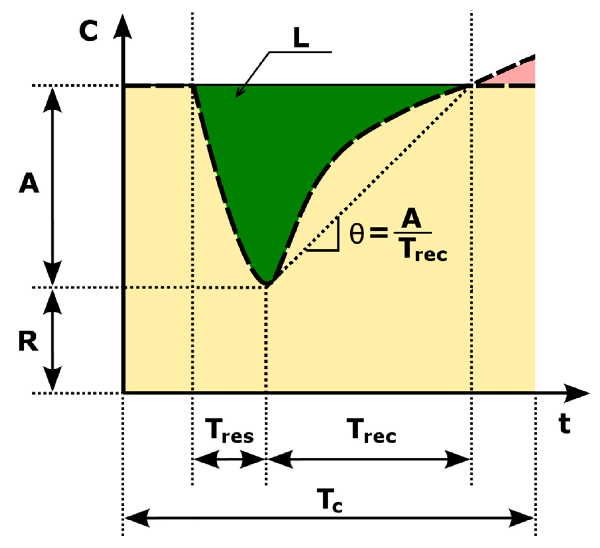
There are various approaches to the formation of system resilience indicators [9,12]. Of those, However, most studies are devoted to the analysis of resilience curves constructed in time coordinates and a system performance indicator, which describe the response of a resilient system to a destructive disturbing influence (Figure 10). The following basic indicators of system resilience were proposed in [9,14,15]:
-
Response Time, Tres;
-
Recovery Time, Trec;
-
Performance Attenuation, A;
-
Performance Loss, L;
-
Robustness, R;
-
Rapidity, θ;
-
Redundancy;
-
Resourcefulness;
-
Іntegrated measure of resilience, Re.
Response Time ( T r e s ) characterizes the timeliness of the response to a destructive disturbance. Systems with short response times are better at mitigating impacts, reducing performance degradation caused by disturbances.
Recovery Time ( T r e c ) is the period required to recover the system functionality to the desired level, at which the system can function in the same way, close to or better than before the disturbance.
Performance Attenuation (A) describes the maximum reduction in system performance as a result of a disturbance, while Loss of Performance (L) characterizes the total loss of performance during the response and recovery phases. The loss of productivity is represented by the area highlighted in darker (green) in Figure 10.
Robustness ( R b ) characterizes the ability of a system to withstand a certain level of stress while maintaining functionality, without significant deterioration or loss of performance. Robustness allows the system to absorb and resist destructive influences. A system with a high degree of robustness will retain most of its functional characteristics under the influence of destructive factors. Robustness can be defined as the residual functionality after exposure to an extreme destructive disturbance and can be calculated using the following formula
R b = 1 A ~ ( m A , σ A ) ,
where A ~ is a random variable expressed as a function of the mean value of m A and the standard deviation σ A for Performance Attenuation indicator.
In [12,13,115], the resilience of AI is defined as robustness, not resilience in the full sense of the word.
Rapidity ( θ ) is the ability to recover functionality in a timely manner, limiting losses and avoiding future failures. Mathematically, the recovery rate is the slope of the performance curve during the recovery period (Figure 10), calculated by the formula
θ = d C ( t ) d t ,
where d/dt is the differentiation operator;
C ( t ) is a function that defines the dependence of performance on time.
The averaged estimate of the Rapidity can be determined by the following formula
θ = A T r e c .
Redundancy characterizes the availability of alternative resources at the recovery stage when primary resources are insufficient. Redundancy is also defined as a measure of the availability of alternative paths in the system structure through which supportive forces can be transferred to ensure stability after the failure of any element [26]. Structural redundancy implies the availability of multiple supporting components that can withstand additional loads in the event of a failure of individual main components. That is, if one or more components fail, the remaining structure is able to redistribute the load and prevent the entire system from failing.
Resourcefulness of the system is the ability to diagnose problems, prioritize and initiate problem solving by identifying and mobilizing material, financial, information, technological and human resources [11]. Resourcefulness and redundancy are closely interrelated, for example, resourcefulness can create redundancies that did not exist before. In addition, resourcefulness and redundancy can affect the speed and time of recovery. Adding resources can reduce the recovery time compared to what would be expected under standard conditions.
Theoretically, if infinite resources were available, the recovery time would asymptotically tend to zero. In practice, even with enormous financial and labor resources, there is a certain minimum recovery time. However, recovery time can be quite long even with a large amount of resources due to inadequate planning, organizational failures, or ineffective policies [16]. Resourcefulness and robustness are also interrelated. It can be argued that investing in limiting initial losses (increasing robustness) may in some cases be the best approach to increasing resilience, as this automatically leads to further reductions in recovery time.
In order to simultaneously take into account time and performance variables when assessing system resilience, various variants of integral indicators have been developed [17,18]. These indicators typically characterize the difference or ratio of nominal performance and performance loss over time due to disturbances. For convenience, the integral resilience indicator can be expressed in a normalized form as:
R 1 E E t = 0 T c C ( t ) d t t = 0 T c C n o min a l ( t ) d t .
C ( t ) is a function of the dependence of the current value of system performance or functionality on time;
C n o min a l ( t ) is the value of the system performance in the normal (nominal) functional state, which is entered into the formula to map the values of the integral resilience indicator to the interval [0,1];
T c is a control period, which is selected based on the results of a preliminary assessment of the average interval between events of disturbance;
E is a set of disturbance events during the control period.
In the case of machine learning, the time axis denotes the amount of training or test data passed through the AIS or the number of iterations, meaning mini-batches of optimal size.
Resilience indicators are evaluated in relation to a certain type of perturbation. In the case of neural networks, typical disturbances are adversarial attacks, faults, and concept drift. At the same time, different weights of neural networks have different importance and impact on AIS performance. In addition, an error in the higher bits of the tensor value leads to a greater distortion of the results than an error in the lower bits. Similarly, the effectiveness of adversarial attacks with the same perturbation level can vary greatly depending on the spatial distribution of the perturbed pixels. Therefore, statistical characteristics should be used to evaluate and compare the resilience of the AIS to corrupted tensors or perturbed data. Such statistical characteristics can beobtained from a large number of experiments. For simplicity, we can consider the median value (MED) and interquartile range (IRQ) of the performance and resilience indicators.
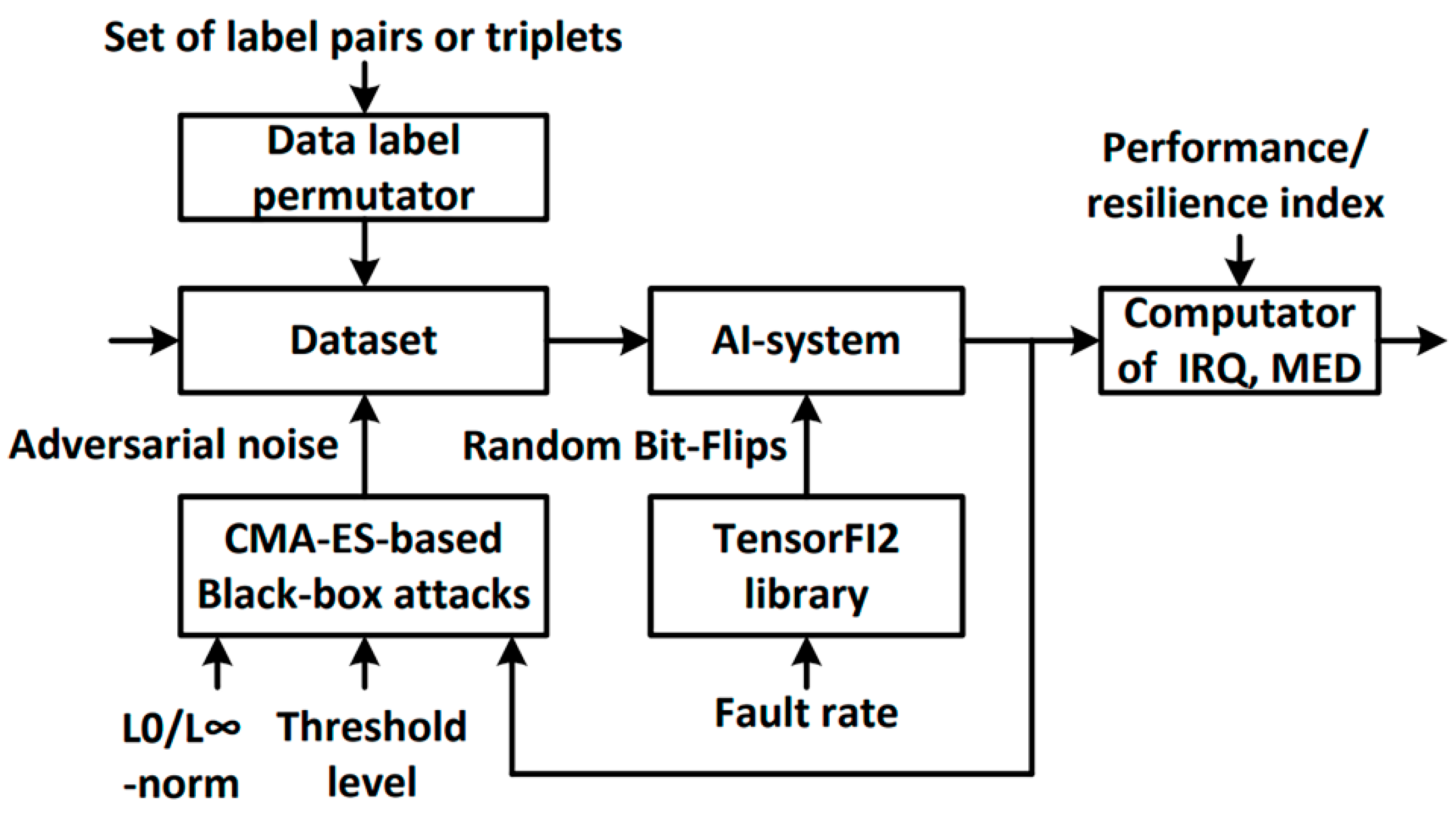
The TensorFI2 library, which is capable of emulating software and hardware failures, has become popular for testing AI for fault tolerance [116]. It has been noted [70] that one of the most difficult types of faults to absorb is the random bit-flip injection into each layer of the model, with a randomly selected fixed fraction of the tensors (failure rate) and one or few randomly selected bit for inversion.
In [30,117], it is proposed not to rely on specific aspects of the model architecture and learning algorithm, such as gradients, to test the model for resistance to noise and adversarial attacks. Instead, testing is based on black box attacks, which expands the family of AIS that can be tested. In this case, there are two types of attacks that give the most diverse results – "strong" attacks on one/few pixels and "weak" attacks on all pixels. The formation of both attacks is realized on the basis of the Covariance matrix adaptation evolution strategy (CMA-ES) [117,118]. For the first type of attacks, the constraint on the perturbation amplitude (th) is given by the L0-norm, and for the second type of attacks, by the L∞-norm.
Testing the model's resilience to drift usually involves the most complex cases of drift, such as the emergence of a new class or real concept drift. The ability to adapt to concept drift can be tested by passing a sample of classes with swapped labels to the model for continual training. Successful adaptation means that performance post-recovery reaches at least 95% of the pre-disturbance performance. The condition for stopping the adaptation process is lack of improving performance within a given number of iterations or reaching the maximum number of steps (mini-batches).
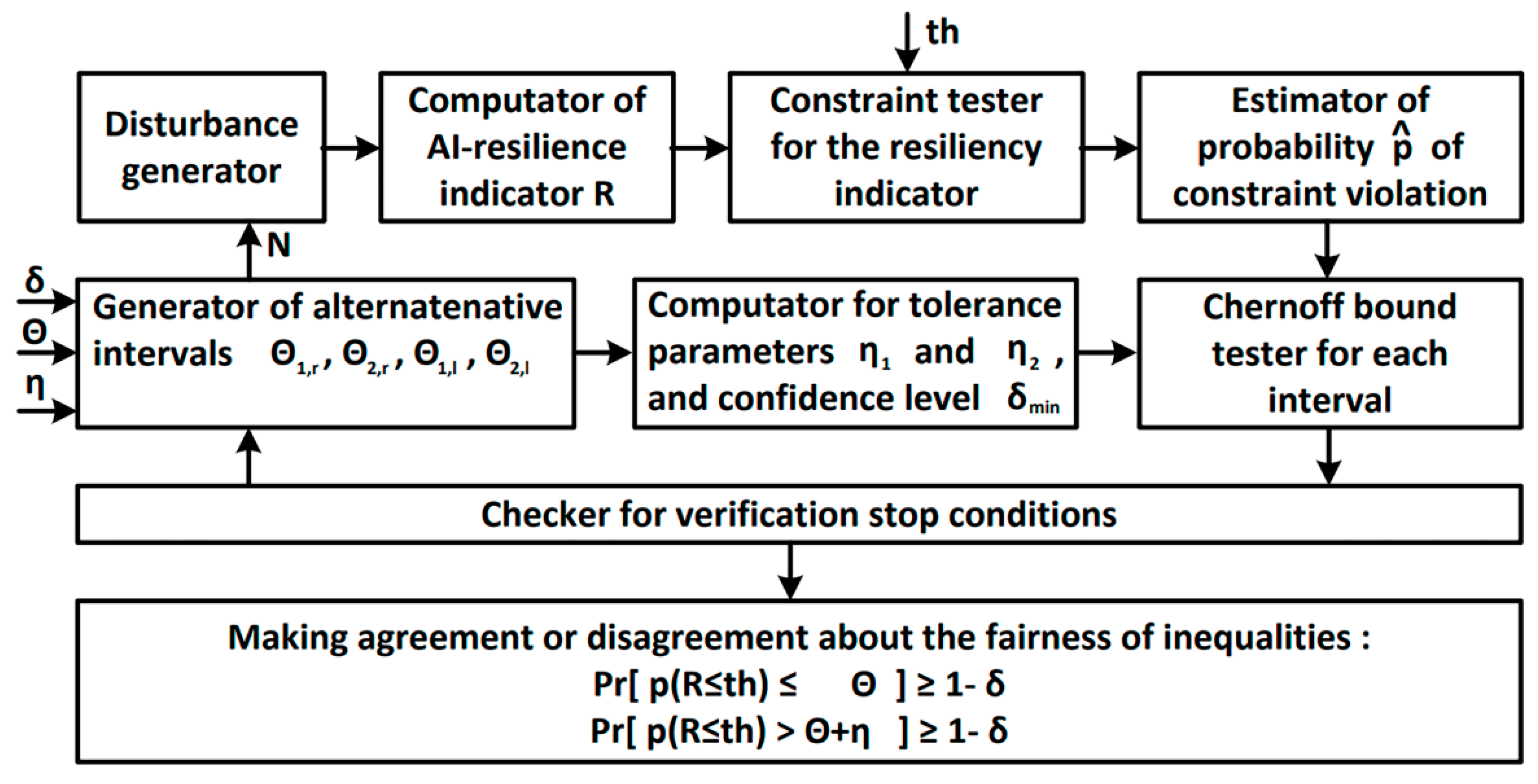
In [30,31,118], the resilience of the image classification system to faults, adversarial attacks, and real concept drift was tested. Figure 11 shows a diagram of the resilience testing method.
In the testing diagram presented in Figure 11 shows, the AIS is considered as a black box. Only information about the AIS inputs and outputs is used, information about gradients AIS is ignored. Testing is performed by generating a disturbance and observing the AIS performance changing during disturbance absorbtion and adaptation. Empirical testing is more suitable for comparative analysis, as an analytical tool in assessing AIS resilience – however, empirical testing does not provide exact guarantees. To increase the effectiveness of empirical testing, it is necessary to improve test coverage. Another disadvantage of empirical testing is the lack of clear quantification of confidence in the truth of the desired property after testing [118,119].
Formal verification methods are used to provide rigorous guarantees of test results. The works related to the formal verification of deep neural networks consider various options for encoding the model in a form convenient for the solver and implemented in accordance with the chosen theory [120,121,122]. The most well-known approaches to formal verification are as follows: constraint solver-based approaches, where the neural network is encoded as a set of constraints [123]; approaches based on the calculation of approximate bounds, where approximation operations are applied to the space of inputs, outputs, or functions of neural layers to simplify the search for guaranteed bounds [124,125]; approaches based on the calculation of converging bounds, where the search and iterative refinement of guaranteed bounds are performed [126,127]. These approaches are designed to provide qualitative verification and rely on deterministic results, but characterized by high computational complexity. However, factors such as the stochastic nature of learning, the appearance of data from an unknown distribution in the inference mode, the development of probabilistic neural networks and randomized model architectures narrow the possibilities and effectiveness of qualitative verification. In response to that, probabilistic (statistical) methods of verification (certification) are being developed; such methods are the most generalised and computationally efficient. An example of such method is the Lipschitz stability estimation method based on the theory of extreme values -but such methods have a reliability problem [128]. In addition, the vast majority of publications only consider verification of AIS robustness to disturbances [130]. Not nearly enough attention is paid to the behavior of the AIS in the performance recovery mode. Recovery speed after a disturbance is still not verified.
The paper [129,130] proposes an approach to black-box probabilistic verification of robustness. An extended version of this approach for the case of the AIS resilience verification problem with reduced requirements for the number of tests is shown in Figure 12. In this case, the resilience to each sample of disturbance is assessed on the basis of a resilience curve, which is plotted over a predetermined interval T, and calculated by the formula (6). Also, before starting the test, the size of the mini-batch needs to be set.
Figure 12. Functional diagram of AIS resilience verification.
Preprints 68606 g012
Verification is carried out for four selected parameters th, θ , η and δ , where th is specified threshold value for the minimum permissible value of the resilience indicator, θ is a specified threshold value for the probability of insufficient resilience, η is the specified tolerance value on probability estimation, δ is a statistical significance, which is usually selected from a set {0,1; 0,05, 0,01; 0,001}.
The agreement of the verification algorithm consists of checking the validity of the following two inequalities:
P r [ p ( R t h ) θ ] 1 δ ;
Pr p R t h > θ + η 1 δ ,
where Pr is the confidence level of assessing the probability of success and non-success in testing the algorithm for insufficient resilience to destructive disturbance;
R is integral indicator of the AIS resilience;
p R t h is an assessed probability of insufficient resilience.
The resilience verification algorithm is based on the Chernoff bounds lemma [130,131]. According to this lemma, to verify the validity of inequalities (7) and (8), it is necessary to perform N tests, where
N = 12 η 2 l n 1 δ .
In [130], in order to reduce the number of tests of the Chernoff boundary in the case of a significant difference between the real probability p(R <= th) and the threshold value θ, a series of alternative hypotheses are considered. Instead of checking inequalities (7) and (8), it is proposed to check a series of alternative inequalities, the verification of which requires fewer tests for early decision-making
P r [ p ( R t h ) θ 1 ] 1 δ m i n ;
Pr p R t h > θ 2 1 δ m i n ,
where θ 1 and θ 2 are boundaries of an alternative interval instead of an interval [ θ , θ + η ];
δ m i n is the statistical significance for one of the n alternative intervals, which can be calculated using the following formula
δ m i n = δ n .
The total number of alternative intervals includes the maximum number of intervals to the left n l from θ , and the maximum number of intervals to the right n r from θ + η . If no decision is made on the alternative intervals, testing is additionally performed for the interval [ θ , θ + η ]:
n l 1 + l o g θ η ,
n r 1 + l o g 1 θ η η ,
n = 3 + max 0 , l o g 2 θ η + max 0 , l o g 2 1 θ η η .
The intervals chosen to the left from θ , can be called confirmatory, since the confirmation of inequalities (10) and (12) at any of these intervals terminates the algorithm with a positive result. The intervals to the right from θ + η can be called refuting, since a negative result of checking inequalities (10) and (11) at any of these intervals terminates the algorithm with a negative result. In order to speed up the algorithm, it is proposed to form the intervals in a reverse size order, from their maximum size to the minimum, where each subsequent interval is formed by dividing the width of the previous interval in half (Figure 13).
Each alternative interval requires N tests to be tested
N = 3 θ 1 + 2 θ 2 2 θ 2 θ 2 2 l n 1 δ m i n ,
where η 1 , η 2 are the permissible tolerances of probability estimation p R t h on a sample of tests of limited size N on the left and right, calculated by the formulas
η 1 = θ 2 θ 1 1 + 2 3 θ 2 θ 1 1 ,
η 2 = θ 2 θ 1 η 1 .
The test on an alternative interval is considered successful if the estimation p ^ of probability p R t h is less than or equal to θ 1 + η 1 . A test on an alternative interval is considered unsuccessful if the estimation p ^ of probability p R t h is greater than θ 2 η 2 . If none of these conditions is met, this indicates the need to continue generating new intervals and continue the testing process. However, the process can also stop if the time or the resource allocated for testing are expired.
Partial or integral AIS resilience indicators depend on the AIS performance indicators. These indicators may be considered as an evaluation metrics of AIS. The evaluation metrics can be optimized in the space of AIS hyperparameters quite simply, but computationally costly [132]. However, the optimization of evaluation metrics in the space of AIS parameter performs indirectly by minimizing the loss function using gradient-based algorithms. Optimization with loss-only supervision may travel through several “bumps” in the metric space, and tends to converge to a suboptimal solution in terms of evaluation metric. However, many evaluation metrics are non-continuous, non-differentiable, or non-decomposable, which poses challenges for direct metric optimization due to the difficulty of obtaining an informative gradients. State-of-the-art approaches addressed to loss-metric mismatch issue are represented in Table 6.
There are many methods of solving the loss-metric mismatch issue from better metric-aligned surrogate losses to Black-box evaluation metrics optimization. The most universal method to optimize black-box evaluation metrics is based on the meta-learned value function. However, this approach has a more complicated protocol for AIS-training. At first, conditional (adapter) parameters are added to the main model to modulate the feature sets of the main model. The main model should be pre-trained using a user-specified surrogate loss and then fine-tuned. At the stage of AIS fine-tuning, calculated values of surrogate loss function and black-box metric are collected. Sparse metric observations are interpolated to match the values of the conditional parameters. Fine-tuning can be performed on a set of optimization problems. Based on the collected data, the function of mapping the conditional parameters to the value of the black-box metric is constructed. After meta-training of value function, the main model can be fine-tuned using the estimates of the black box metric. Hence, the value function is differentiable and provide useful supervision or gradients for black-box metric.

4. Open Challenges and Conclusions

Throughout this survey various publications related to AI resilience have been discussed. Concepts of AI and resilience are very known and dynamically developing during the 21 centure in terms of methodlogy, models, and technologies. However, until the last decade, these concepts inverstigated independently and almost did not overlap. This state of affairs was somewhat unnatural, since in their essence these concepts are quite close. AISs have to be resilient by definition, because they as “traditional” (non-AI) systems should take into account the changes of the information and physical environment parameters, the evolutional changes of requirements, and the occurrence of unspecified failures caused by hardware and software faults and cyber attacks.
However, compared to traditional systems, where resilience is primarily related to proactive failure and intrusion tolerance, AISs can more “naturally” change their properties and algorithms of functioning in unusual conditions. For that they must be developed, trained, and applied accordingly. In this article, we tried to systematize just such specific mechanisms for ensuring the resilience of AI and AISs.
The ontological and taxonomic diagrams of AIS vulnerabilities and resilience were constructed to systematize knowledge about this topic. The approaches and methods of ensuring specific stages of resilience to handling faults, drift and adversarial attacks have been analyzed. The basic ideas and principles of measuring, certifying and optimizing AIS resilience are considered. It had been shown that particular resilience properties can be built into cutting edge AIS, by implementing some of the techniques discussed.
The vast majority of scientific research is aimed at analyzing a specific type of disturbance and the defense mechanism against it. There are virtually no studies considering the combination of two or more types or subtypes of AIS disturbances. However, not all methods of ensuring fault tolerance are compatible with methods of ensuring resilience to adversarial attacks. For example, [144] shows that adversarial training increases robustness to noisy data, but simultaneously reduces the fault tolerance obtained by fault-tolerant training. Also, not all methods of ensuring resilience to concept drift are compatible with methods of ensuring resilience to adversarial attacks. For example, [145] shows that the use of unsupervised domain adaptation reduces the resilience of AIS to evasive adversarial attacks, which necessitates special solutions to simultaneously ensure adversarial robustness. Moreover, methods that implement different stages of resilience to the same type of disturbance may interfere with each other, i.e., may not be completely compatible. For example, disturbance absorption methods based on the diversity property of an ensemble or a family of models are logically incompatible with methods of graceful degradation and adaptation based on increasing the representation power of a neural network. In addition to the problem of compatibility, there may be a problem of resource inefficiency from combining separate methods. For example, if regularization-based continual learning based on center-loss or contrastive center loss is used to adapt AIS to changing environments [59,146], then the implementation of the disturbance absorption stage should also be carried out using similar regularizations, rather than using defensive distillation [52,59], since distillation will add computational costs without additional benefits. All these aspects need to be studied in more detail to implement all stages of affordable resilience to the complex impact of disturbances of various types and subtypes.
A number of criteria for measuring the qualitative characteristics of AIS, including the components of resilience had been developed [147]. However, many of these criteria depend on either the type of AIS task or the type of AI model. The more high-level the criterion is, the fewer methods there are for its direct optimization during machine learning. The majority of methods for addressing the loss-metric mismatch require the development of surrogate loss functions, meta-learning, and changes or add-ons to the main AI model [142,143]. It is known that ensuring robustness, adaptation rate, and performance is somewhat contradictory [148]. There is a need for a tradeoff approach when optimizing AIS. The problem of optimizing the integral resilience criterion of AIS, which takes into account not only the robustness of the system but also the ability to quickly recover and adapt, is still not fully resolved and remains relevant [31,118]. In practice, it is necessary to be able not only to measure the resilience of AIS to a specific disturbance event, but also to provide certain guarantees to ensure resilience not lower than a certain level to a whole class of disturbances of a certain intensity. Existing approaches are characterized by high computational costs, and the issue of reducing the cost of such guarantee is relevant [129,130].
The vast majority of methods for ensuring certain resilience characteristics involve significant changes to the architecture or training algorithm of AIS. On one hand, this stimulates the progress of AI-technology and the development of best practices for AIS design, but on the other hand, it complicates the unification of technologies to ensure AIS resilience [6,150]. From the business point of view, the idea of creating AIS resiliency services independent of the task and model is attractive [149,150]. The ability to provide resilience as a service for AIS could become an integral part of MLOps platforms' tools, which would reduce the operational costs of AI-based services.
Future research should focus on the development of criteria, models, and methods for model-agnostic and task-agnostic measurement, optimization and verification of AIS resilience. Special attention should also be paid to the question of providing resilience as service for AIS of various types and complexity. Another important direction of research should be the investigation and creation of explainable and trustworthy AI components for more complex self-organizing systems of knowledge representation and development [151]. In such systems, models of the interaction of various AI components and subsystems must be developed for the general purpose of resilient functioning and self-organization.

Author Contributions

V.M.: writing – original draft preparation; A.M., B.K.: writing – review and editing; V.K.: supervision and revision. All authors have read and agreed to the published version of the manuscript.

Funding

This research received no external funding.

Institutional Review Board Statement

Not applicable.

Informed Consent Statement

Informed consent was obtained from all subjects involved in the study.

Data Availability Statement

Not applicable.

Acknowledgments

The authors appreciate the scientific society of the consortium and, in particular, the staff of the Department of Computer Systems, Networks and Cybersecurity (DCSNCS) at the National Aerospace University “KhAI” and the Laboratory of Intellectual Systems (LIS) of the Computer Science Department at the Sumy State University for invaluable inspiration, hard work, and creative analysis during the preparation of this paper. In addition, the authors thanks Ministry of Education and Science of Ukraine for the support to the LIS in the framework of research project No 0122U000782 “Information technology for providing resilience of artificial intelligence systems to protect cyber-physical systems” (2022-2024) and the support of project No 0122U001065 ‘Dependability assurance methods and technologies for intellectual industrial IoT systems” (2022-2023) implemented by the DCSNCS.

Conflicts of Interest

The authors declare no conflict of interest.

References

  1. Xu, J.; Kovatsch, M.; Mattern, D.; Mazza, F.; Harasic, M.; Paschke, A.; Lucia, S. A Review on AI for Smart Manufacturing: Deep Learning Challenges and Solutions. Appl. Sci. 2022, 12(16), 8239. [CrossRef]
  2. Khalid, F.; Hanif, M. A.; Shafique, M. Exploiting Vulnerabilities in Deep Neural Networks: Adversarial and Fault-Injection Attacks. CoRR. 2021. abs/2105.03251. [CrossRef]
  3. Gongye, C.; Li, H.; Zhang, X.; Sabbagh, M.; Yuan, G.; Lin, X.; Wahl, T.; Fei, Y. New passive and active attacks on deep neural networks in medical applications. In ICCAD '20: IEEE/ACM International Conference on Computer-Aided Design, Virtual Event USA; ACM: New York, NY, USA, 2020. [CrossRef]
  4. Caccia, M.; Rodríguez, P.; Ostapenko, O.; Normandin, F.; Lin, M.; Caccia, L.; Laradji, I.; Rish, I.; Lacoste, A.; Vazquez, D.; et al. Online fast adaptation and knowledge accumulation (OSAKA): A new approach to continual learning. In Proceedings of the 34th International Conference on Neural Information Processing Systems, Vancouver, BC, Canada, 6–12 Dec 2020; pp. 16532–16545.
  5. Margatina, K.; Vernikos, G.; Barrault, L.; Aletras, N. Active learning by acquiring contrastive examples. https://arxiv.org/abs/2109.03764 (accessed Feb 9, 2023).
  6. Parisi, G. I.; Kemker, R.; Part, J. L.; Kanan, C.; Wermter, S. Continual Lifelong Learning with Neural Networks: A Review. Neural Networks 2019, 113, 54–71. [CrossRef]
  7. Ruf, P.; Madan, M.; Reich, C.; Ould-Abdeslam, D. Demystifying Mlops and Presenting a Recipe for the Selection of Open-Source Tools. Applied Sciences 2021, 11 (19), 8861. [CrossRef]
  8. Ghavami, B.; Sadati, M.; Fang, Z.; Shannon, L. FitAct: Error Resilient Deep Neural Networks via Fine-Grained Post-Trainable Activation Functions. 2022 Design, Automation & Test in Europe Conference & Exhibition (DATE) 2022. [CrossRef]
  9. Yin, Y.; Zheng, X.; Du, P.; Liu, L.; Ma, H. Scaling Resilient Adversarial Patch. 2021 IEEE 18th International Conference on Mobile Ad Hoc and Smart Systems (MASS) 2021. pp. 189-197 . [CrossRef]
  10. Guo, H.; Zhang, S.; Wang, W. Selective Ensemble-Based Online Adaptive Deep Neural Networks for Streaming Data with Concept Drift. Neural Networks 2021, 142, 437–456. [CrossRef]
  11. Fraccascia, L.; Giannoccaro, I.; Albino, V. Resilience of Complex Systems: State of the Art and Directions for Future Research. Complexity. 2018, 2018, 3421529. [CrossRef]
  12. Ruospo, A.; Sanchez, E.; Luza, L. M.; Dilillo, L.; et al. A Survey on Deep Learning Resilience Assessment Methodologies. Computer. 2022. 1-11.
  13. He, Y.; Balaprakash, P.; Li, Y. FIdelity: Efficient Resilience Analysis Framework for Deep Learning Accelerators. У 2020 53rd Annual IEEE/ACM International Symposium on Microarchitecture (MICRO), Athens, Greece, 17–21 Oct 2020; IEEE, 2020. [CrossRef]
  14. Santos, S. G. T. d. C.; Gonçalves Júnior, P. M.; Silva, G. D. d. S.; de Barros, R. S. M. Speeding Up Recovery from Concept Drifts. У Machine Learning and Knowledge Discovery in Databases; Springer Berlin Heidelberg: Berlin, Heidelberg, 2014;p. 179–194. [CrossRef]
  15. Lusenko, S.; Kharchenko, V.; Bobrovnikova, K.; Shchuka, R. Computer systems resilience in the presence of cyber threats: taxonomy and ontology. Radioelectronic and computer systems. 2020, 1, 17–28. [CrossRef]
  16. Drozd, O.; Kharchenko, V.; Rucinski, A.; Kochanski, T.; Garbos, R.; Maevsky, D. Development of Models in Resilient Computing. In 2019 10th International Conference on Dependable Systems, Services and Technologies (DESSERT), Leeds, United Kingdom, 5–7 Jun 2019; IEEE, 2019. [CrossRef]
  17. Allenby, B.; Fink, J. Toward Inherently Secure and Resilient Societies. Science 2005, 309 (5737), 1034–1036. [CrossRef]
  18. Haimes, Y. Y. On the Definition of Resilience in Systems. Risk Analysis 2009, 29 (4), 498–501. [CrossRef]
  19. Vugrin, E. D.; Warren, D. E.; Ehlen, M. A.; Camphouse, R. C. A Framework for Assessing the Resilience of Infrastructure and Economic Systems. Sustainable and Resilient Critical Infrastructure Systems 2010, 77–116. [CrossRef]
  20. Cimellaro, G. P.; Reinhorn, A. M.; Bruneau, M. Framework for Analytical Quantification of Disaster Resilience. Engineering Structures 2010, 32 (11), 3639–3649. [CrossRef]
  21. Fairbanks, R. J.; Wears, R. L.; Woods, D. D.; Hollnagel, E.; Plsek, P.; Cook, R. I. Resilience and Resilience Engineering in Health Care. The Joint Commission Journal on Quality and Patient Safety 2014, 40 (8), 376–383. [CrossRef]
  22. Yodo, N.; Wang, P. Engineering Resilience Quantification and System Design Implications: A Literature Survey. Journal of Mechanical Design 2016, 138 (11). [CrossRef]
  23. Brtis, J. S.; McEvilley, M. A.; Pennock, M. J. Resilience Requirements Patterns. INCOSE International Symposium 2021, 31 (1), 570–584. [CrossRef]
  24. Barker, K.; Lambert, J. H.; Zobel, C. W.; Tapia, A. H.; Ramirez-Marquez, J. E.; Albert, L.; Nicholson, C. D.; Caragea, C. Defining resilience analytics for interdependent cyber-physical-social networks. Sustainable and Resilient Infrastructure 2017, 2 (2), 59–67. [CrossRef]
  25. Cutter, S. L.; Ahearn, J. A.; Amadei, B.; Crawford, P.; Eide, E. A.; Galloway, G. E.; Goodchild, M. F.; Kunreuther, H. C.; Li-Vollmer, M.; Schoch-Spana, M. Disaster Resilience: A National Imperative. Environment: Science and Policy for Sustainable Development 2013, 55 (2), 25–29. [CrossRef]
  26. Madni, A. M. Affordable Resilience. In Transdisciplinary Systems Engineering; Springer International Publishing: Cham, 2017; p. 133–159. [CrossRef]
  27. Crespi, B. J. Cognitive trade-offs and the costs of resilience. Behavioral and Brain Sciences 2015, 38. [CrossRef]
  28. Dyer, J. S. Multiattribute Utility Theory (MAUT). У Multiple Criteria Decision Analysis; Springer New York: New York, NY, 2016; p. 285–314. [CrossRef]
  29. Kulakowski, K. Understanding Analytic Hierarchy Process; Taylor & Francis Group, 2020. [CrossRef]
  30. Moskalenko, V. V.; Moskalenko, A. S.; Korobov, A. G.; Zaretsky, M. O. Image Classifier Resilient To Adversarial Attacks, Fault Injections And Concept Drift – Model Architecture And Training Algorithm. Radio Electronics, Computer Science, Control 2022, (3), 86. [CrossRef]
  31. Moskalenko, V.; Moskalenko, A. Neural network based image classifier resilient to destructive perturbation influences – architecture and training method. Radioelectronic and computer systems 2022, (3), 95–109. [CrossRef]
  32. Eggers, S.; Sample, C. Vulnerabilities in Artificial Intelligence and Machine Learning Applications and Data; Office of Scientific and Technical Information (OSTI), Dec 2020. [CrossRef]
  33. Tabassi, E. A Taxonomy and Terminology of Adversarial Machine Learning; National Institute of Standards and Technology: Gaithersburg, MD, 2023. [CrossRef]
  34. Torres-Huitzil, C.; Girau, B. Fault and Error Tolerance in Neural Networks: A Review. IEEE Access 2017, 5, 17322–17341. [CrossRef]
  35. Agrahari, S.; Singh, A. K. Concept Drift Detection in Data Stream Mining : A literature review. Journal of King Saud University – Computer and Information Sciences 2021. [CrossRef]
  36. Museba, T.; Nelwamondo, F.; Ouahada, K. ADES: A New Ensemble Diversity-Based Approach for Handling Concept Drift. Mobile Information Systems 2021, 2021, 1–17. [CrossRef]
  37. Malekzadeh, E.; Rohbani, N.; Lu, Z.; Ebrahimi, M. The Impact of Faults on DNNs: A Case Study. У 2021 IEEE International Symposium on Defect and Fault Tolerance in VLSI and Nanotechnology Systems (DFT), Athens, Greece, 6–8 Oct 2021; IEEE, 2021. [CrossRef]
  38. Benevenuti, F.; Libano, F.; Pouget, V.; Kastensmidt, F. L.; Rech, P. Comparative Analysis of Inference Errors in a Neural Network Implemented in SRAM-Based FPGA Induced by Neutron Irradiation and Fault Injection Methods. У 2018 31st Symposium on Integrated Circuits and Systems Design (SBCCI), Bento Goncalves, 27–31 Aug 2018; IEEE, 2018. [CrossRef]
  39. Li, J.; Rakin, A. S.; Xiong, Y.; Chang, L.; He, Z.; Fan, D.; Chakrabarti, C. Defending Bit-Flip Attack through DNN Weight Reconstruction. In 2020 57th ACM/IEEE Design Automation Conference (DAC), San Francisco, CA, USA, 20–24 Jul 2020; IEEE, 2020. [CrossRef]
  40. Akhtar, N.; Mian, A. Threat of Adversarial Attacks on Deep Learning in Computer Vision: A Survey. IEEE Access 2018, 6, 14410–14430. [CrossRef]
  41. Zhou, S.; Liu, C.; Ye, D.; Zhu, T.; Zhou, W.; Yu, P. S. Adversarial Attacks and Defenses in Deep Learning: from a Perspective of Cybersecurity. ACM Computing Surveys 2022. [CrossRef]
  42. Khalid, F.; Ali, H.; Abdullah Hanif, M.; Rehman, S.; Ahmed, R.; Shafique, M. FaDec: A Fast Decision-based Attack for Adversarial Machine Learning. In 2020 International Joint Conference on Neural Networks (IJCNN), Glasgow, United Kingdom, 19–24 Jul 2020; IEEE, 2020. [CrossRef]
  43. Altoub, M.; AlQurashi, F.; Yigitcanlar, T.; Corchado, J. M.; Mehmood, R. An Ontological Knowledge Base of Poisoning Attacks on Deep Neural Networks. Applied Sciences 2022, 12 (21), 11053. [CrossRef]
  44. Chakraborty, A.; Alam, M.; Dey, V.; Chattopadhyay, A.; Mukhopadhyay, D. A survey on adversarial attacks and defences. CAAI Transactions on Intelligence Technology 2021, 6 (1), 25–45. [CrossRef]
  45. Zona, A.; Kammouh, O.; Cimellaro, G. P. Resourcefulness quantification approach for resilient communities and countries. International Journal of Disaster Risk Reduction 2020, 46, 101509. [CrossRef]
  46. Eigner, O.; Eresheim, S.; Kieseberg, P.; Klausner, L. D.; Pirker, M.; Priebe, T.; Tjoa, S.; Marulli, F.; Mercaldo, F. Towards Resilient Artificial Intelligence: Survey and Research Issues. У 2021 IEEE International Conference on Cyber Security and Resilience (CSR), Rhodes, Greece, 26–28 Jul 2021; IEEE, 2021. [CrossRef]
  47. Olowononi, F. O.; Rawat, D. B.; Liu, C. Resilient Machine Learning for Networked Cyber Physical Systems: A Survey for Machine Learning Security to Securing Machine Learning for CPS. IEEE Communications Surveys & Tutorials 2020, 1. [CrossRef]
  48. Graceful degradation and related fields - ePrints Soton. Welcome to ePrints Soton - ePrints Soton. https://eprints.soton.ac.uk/455349/ (accessed on 11.02.2023).
  49. Hoang, L.-H.; Hanif, M. A.; Shafique, M. TRe-Map: Towards Reducing the Overheads of Fault-Aware Retraining of Deep Neural Networks by Merging Fault Maps. In 2021 24th Euromicro Conference on Digital System Design (DSD), Palermo, Italy, 1–3 Sept 2021; IEEE, 2021. [CrossRef]
  50. Xie, C.; Wang, J.; Zhang, Z.; Ren, Z.; Yuille, A. Mitigating Adversarial Effects Through Randomization. In Proceedings of the International Conference on Learning Representations, Toulon, France, 24–26 April 2017; pp. 1–16. https://arxiv.org/abs/1711.01991.
  51. Athalye, A.; Carlini, N.; Wagner, D. Obfuscated Gradients Give a False Sense of Security: Circumventing Defenses to Adversarial Examples. CoRR 2018, abs/1802.00420. [CrossRef]
  52. Papernot, N.; McDaniel, P.; Wu, X.; Jha, S.; Swami, A. Distillation as a Defense to Adversarial Perturbations Against Deep Neural Networks. In 2016 IEEE Symposium on Security and Privacy (SP), San Jose, CA, 22–26 May 2016; IEEE, 2016. [CrossRef]
  53. Srisakaokul, S.; Zhong, Z.; Zhang, Y.; Ti, B.; Xie, T.; Yang, W. Multi-Model-Based Defense Against Adversarial Examples for Neural Networks. CoRR 2018, abs/1809.00065. [CrossRef]
  54. Song, Y.; Kim, T.; Nowozin, S.; Ermon, S.; Kushman, N. PixelDefend: Leveraging Generative Models to Understand and Defend against Advers arial Examples. In Proceedings of the International Conference on Learning Representations, Vancouver, QC, Canada, 30 April–3 May 2018; pp. 1–20. https://arxiv.org/abs/1710.10766.
  55. Samangouei, P.; Kabkab, M.; Chellappa, R. Protecting Classifiers Against Adversarial Attacks Using Generative Models. CoRR 2018, abs/1805.06605. [CrossRef]
  56. Makarichev, V.; Lukin, V.; Illiashenko, O.; Kharchenko, V. Digital Image Representation by Atomic Functions: The Compression and Protection of Data for Edge Computing in IoT Systems. Sensors 2022, 22 (10), 3751. [CrossRef]
  57. Laermann, J.; Samek, W.; Strodthoff, N. Achieving Generalizable Robustness of Deep Neural Networks by Stability Training. In Lecture Notes in Computer Science; Springer International Publishing: Cham, 2019; pp. 360–373. [CrossRef]
  58. Jakubovitz, D.; Giryes, R. Improving DNN Robustness to Adversarial Attacks using Jacobian Regularization. In Proceedings of the European Conference on Computer Vision, Munich, Germany, 8–14 Sept 2018; pp. 1–16. https://arxiv.org/abs/1803.08680.
  59. Leslie, N.S. A useful taxonomy for adversarial robustness of Neural Networks. Trends Comput. Sci. Inf. Technol. 2020, 5, 37–41. [CrossRef]
  60. Shu, X.; Tang, J.; Qi, G.-J.; Li, Z.; Jiang, Y.-G.; Yan, S. Image Classification with Tailored Fine-Grained Dictionaries. IEEE Trans. Circuits Syst. Video Technol. 2018, 28, 454–467. [CrossRef]
  61. Deng, Z.; Yang, X.; Xu, S.; Su, H.; Zhu, J. LiBRe: A Practical Bayesian Approach to Adversarial Detection. In Proceedings of the IEEE/CVF Conference on Computer Vision and Pattern Recognition (CVPR), Nashville, TN, USA, 20–25 June 2021; pp. 972–982. [CrossRef]
  62. Abusnaina, A.; Wu, Y.; Arora, S.; Wang, Y.; Wang, F.; Yang, H.; Mohaisen, D. Adversarial Example Detection Using Latent Neighborhood Graph. In Proceedings of the IEEE/CVF International Conference on Computer Vision (ICCV), Montreal, QC, Canada, 10–17 October 2021. [CrossRef]
  63. Venkatesan, S.; Sikka, H.; Izmailov, R.; Chadha, R.; Oprea, A.; de Lucia, M. J. Poisoning Attacks and Data Sanitization Mitigations for Machine Learning Models in Network Intrusion Detection Systems. У MILCOM 2021 - 2021 IEEE Military Communications Conference (MILCOM), San Diego, CA, USA, 29 листoпада–2 грудня 2021; IEEE, 2021. [CrossRef]
  64. Carlini, N.; Wagner, D. Adversarial Examples Are Not Easily Detected. In Proceedings of the 10th ACM Workshop on Artificial Intelligence and Security, Dallas, TX, USA, 3 November 2017; pp. 3–14. [CrossRef]
  65. Zhao, W.; Alwidian, S.; Mahmoud, Q. H. Adversarial Training Methods for Deep Learning: A Systematic Review. Algorithms 2022, 15 (8), 283. [CrossRef]
  66. Xu, J.; Li, Z.; Du, B.; Zhang, M.; Liu, J. Reluplex made more practical: Leaky ReLU. In Proceedings of the IEEE Symposium on Computers and Communications (ISCC), Rennes, France, 7–10 July 2020; pp. 1–6. [CrossRef]
  67. Carrara, F.; Becarelli, R.; Caldelli, R.; Falchi, F.; Amato, G. Adversarial Examples Detection in Features Distance Spaces. In Physics of Solid Surfaces; Springer: Berlin/Heidelberg, Germany, 2019; pp. 313–327. [CrossRef]
  68. Jang, M.; Hong, J. MATE: Memory- and Retraining- Free Error Correction for Convolutional Neural Network Weights. J. Lnf. Commun. Converg. Eng. 2021, 19, 22–28. [CrossRef]
  69. Li, W.; Ning, X.; Ge, G.; Chen, X.; Wang, Y.; Yang, H. FTT-NAS: Discovering Fault-Tolerant Neural Architecture. In Proceedings of the 25th Asia and South Pacific Design Automation Conference (ASP-DAC), Beijing, China, 13–16 January 2020; pp. 211–216. [CrossRef]
  70. Hoang, L.-H.; Hanif, M.A.; Shafique, M. TRe-Map: Towards Reducing the Overheads of Fault-Aware Retraining of Deep Neural Networks by Merging Fault Maps. In Proceedings of the 24th Euromicro Conference on Digital System Design (DSD), Palermo, Italy, 1–3 Sept 2021; pp. 434–441. [CrossRef]
  71. Baek, I.; Chen, W.; Zhu, Z.; Samii, S.; Rajkumar, R. R. FT-DeepNets: Fault-Tolerant Convolutional Neural Networks with Kernel-based Duplication. In 2022 IEEE/CVF Winter Conference on Applications of Computer Vision (WACV), Waikoloa, HI, USA, 3–8 Jan 2022; IEEE, 2022. [CrossRef]
  72. Xu, H.; Chen, Z.; Wu, W.; Jin, Z.; Kuo, S.-y.; Lyu, M. NV-DNN: Towards Fault-Tolerant DNN Systems with N-Version Programming. У 2019 49th Annual IEEE/IFIP International Conference on Dependable Systems and Networks Workshops (DSN-W), Portland, OR, USA, 24–27 Jun 2019; IEEE, 2019. [CrossRef]
  73. Liu, T.; Wen, W.; Jiang, L.; Wang, Y.; Yang, C.; Quan, G. A Fault-Tolerant Neural Network Architecture. In DAC '19: The 56th Annual Design Automation Conference 2019, Las Vegas NV USA; ACM: New York, NY, USA, 2019. [CrossRef]
  74. Huang, K.; Siegel, P. H.; Jiang, A. Functional Error Correction for Robust Neural Networks. IEEE Journal on Selected Areas in Information Theory 2020, 1 (1), 267–276. [CrossRef]
  75. Li, J.; Rakin, A.S.; He, Z.; Fan, D.; Chakrabarti, C. RADAR: Run-time Adversarial Weight Attack Detection and Accuracy Recovery. In Proceedings of the Design, Automation & Test in Europe Conference & Exhibition (DATE), Grenoble, France, 1–5 February 2021; pp. 790–795. [CrossRef]
  76. Wang, C.; Zhao, P.; Wang, S.; Lin, X. Detection and recovery against deep neural network fault injection attacks based on contrastive learning. In Proceedings of the 3rd Workshop on Adversarial Learning Methods for Machine Learning and Data Mining at KDD, Singapore, 14 August 2021; pp. 1–5.
  77. Javaheripi, M.; Koushanfar, F. HASHTAG: Hash Signatures for Online Detection of Fault-Injection Attacks on Deep Neural Networks. In Proceedings of the IEEE/ACM International Conference on Computer Aided Design (ICCAD), Munich, Germany, 1–4 November 2021; pp. 1–9. [CrossRef]
  78. Valtchev, S.Z.; Wu, J. Domain randomization for neural network classification. J. Big Data 2021, 8, 1–12. [CrossRef]
  79. Volpi, R.; Namkoong, H.; Sener, O.; Duchi, J.; Murino, V.; Savarese, S. Generalizing to unseen domains via adversarial data augmentation. In Proceedings of the 32nd International Conference on Neural Information Processing Systems, Montréal, QC, Canada, 2–8 December 2018; pp. 1–11. [CrossRef]
  80. Xu, Q.; Yao, L.; Jiang, Z.; Jiang, G.; Chu, W.; Han, W.; Zhang, W.; Wang, C.; Tai, Y. DIRL: Domain-Invariant Representation Learning for Generalizable Semantic Segmentation. In Proceedings of the AAAI Conference on Artificial Intelligence, Palo Alto, CA, USA, 22 February–3 March 2022; pp. 2884–2892. [CrossRef]
  81. Tang, J.; Shu, X.; Li, Z.; Qi, G.-J.; Wang, J. Generalized Deep Transfer Networks for Knowledge Propagation in Heterogeneous Domains. ACM Trans. Multimedia Comput. Commun. Appl. 2016, 12, 1–22. [CrossRef]
  82. Jiao, B.; Guo, Y.; Gong, D.; Chen, Q. Dynamic Ensemble Selection for Imbalanced Data Streams With Concept Drift. IEEE Transactions on Neural Networks and Learning Systems 2022, 1–14. [CrossRef]
  83. Barddal, J. P.; Gomes, H. M.; Enembreck, F.; Pfahringer, B. A survey on feature drift adaptation: Definition, benchmark, challenges and future directions. Journal of Systems and Software 2017, 127, 278–294. [CrossRef]
  84. Goldenberg, I.; Webb, G. I. Survey of distance measures for quantifying concept drift and shift in numeric data. Knowledge and Information Systems 2018, 60 (2), 591–615. [CrossRef]
  85. Wang, P.; Woo, W.; Jin, N.; Davies, D. Concept Drift Detection by Tracking Weighted Prediction Confidence of Incremental Learning. In IVSP 2022: 2022 4th International Conference on Image, Video and Signal Processing, Singapore Singapore; ACM: New York, NY, USA, 2022. [CrossRef]
  86. Lu, J.; Liu, A.; Dong, F.; Gu, F.; Gama, J.; Zhang, G. Learning under Concept Drift: A Review. IEEE Transactions on Knowledge and Data Engineering 2018, 1. [CrossRef]
  87. Demšar, J.; Bosnić, Z. Detecting concept drift in data streams using model explanation. Expert Systems with Applications 2018, 92, 546–559. [CrossRef]
  88. Huang, D. T. J.; Koh, Y. S.; Dobbie, G.; Bifet, A. Drift Detection Using Stream Volatility. In Machine Learning and Knowledge Discovery in Databases; Springer International Publishing: Cham, 2015; p 417–432. [CrossRef]
  89. Wu, J.; Zhang, T.; Zha, Z.-J.; Luo, J.; Zhang, Y.; Wu, F. Self-Supervised Domain-Aware Generative Network for Generalized Zero-Shot Learning. In 2020 IEEE/CVF Conference on Computer Vision and Pattern Recognition (CVPR), Seattle, WA, USA, 13–19 Jun 2020; IEEE, 2020. [CrossRef]
  90. Abdar, M.; Pourpanah, F.; Hussain, S.; Rezazadegan, D.; Liu, L.; Ghavamzadeh, M.; Fieguth, P.; Cao, X.; Khosravi, A.; Acharya, U. R.; et al. A review of uncertainty quantification in deep learning: Techniques, applications and challenges. Information Fusion 2021, 76, 243–297. [CrossRef]
  91. Karimi, D.; Gholipour, A. Improving Calibration and Out-of-Distribution Detection in Deep Models for Medical Image Segmentation. IEEE Transactions on Artificial Intelligence 2022, 1. [CrossRef]
  92. Shao, Z.; Yang, J.; Ren, S. Calibrating Deep Neural Network Classifiers on Out-of-Distribution Datasets. CoRR 2020, abs/2006.08914. [CrossRef]
  93. Achddou, R.; Di Martino, J. M.; Sapiro, G. Nested Learning for Multi-Level Classification. У ICASSP 2021 - 2021 IEEE International Conference on Acoustics, Speech and Signal Processing (ICASSP), Toronto, ON, Canada, 6–11 Jun 2021; IEEE, 2021. [CrossRef]
  94. Huo, Y.; Lu, Y.; Niu, Y.; Lu, Z.; Wen, J.-R. Coarse-to-Fine Grained Classification. У SIGIR '19: The 42nd International ACM SIGIR Conference on Research and Development in Information Retrieval, Paris France; ACM: New York, NY, USA, 2019. [CrossRef]
  95. Pourpanah, F.; Abdar, M.; Luo, Y.; Zhou, X.; Wang, R.; Lim, C. P.; Wang, X.-Z.; Wu, Q. M. J. A Review of Generalized Zero-Shot Learning Methods. IEEE Transactions on Pattern Analysis and Machine Intelligence 2022, 1–20. [CrossRef]
  96. Chen, K.-Y.; Yeh, M.-C. Generative and Adaptive Multi-Label Generalized Zero-Shot Learning. In 2022 IEEE International Conference on Multimedia and Expo (ICME), Taipei, Taiwan, 18–22 Jul 2022; IEEE, 2022. [CrossRef]
  97. Baier, L.; Kühl, N.; Satzger, G.; Hofmann, M.; Mohr, M. Handling Concept Drifts in Regression Problems – the Error Intersection Approach. In WI2020 Zentrale Tracks; GITO Verlag, 2020; pp 210–224. [CrossRef]
  98. Zhang, L.; Bao, C.; Ma, K. Self-Distillation: Towards Efficient and Compact Neural Networks. IEEE Transactions on Pattern Analysis and Machine Intelligence 2021, 1. [CrossRef]
  99. Laskaridis, S.; Kouris, A.; Lane, N. D. Adaptive Inference through Early-Exit Networks. In MobiSys '21: The 19th Annual International Conference on Mobile Systems, Applications, and Services, Virtual WI USA; ACM: New York, NY, USA, 2021. [CrossRef]
  100. Kirk, R.; Zhang, A.; Grefenstette, E.; Rocktäschel, T. A Survey of Zero-shot Generalisation in Deep Reinforcement Learning. Journal of Artificial Intelligence Research 2023, 76, 201–264. [CrossRef]
  101. Fdez-Díaz, M.; Quevedo, J. R.; Montañés, E. Target inductive methods for zero-shot regression. Information Sciences 2022, 599, 44–63. [CrossRef]
  102. Liu, S.; Chen, J.; Pan, L.; Ngo, C.-W.; Chua, T.-S.; Jiang, Y.-G. Hyperbolic Visual Embedding Learning for Zero-Shot Recognition. In 2020 IEEE/CVF Conference on Computer Vision and Pattern Recognition (CVPR), Seattle, WA, USA, 13–19 Jun 2020; IEEE, 2020. [CrossRef]
  103. Shah, K.; Manwani, N. Online Active Learning of Reject Option Classifiers. Proceedings of the AAAI Conference on Artificial Intelligence 2020, 34 (04), 5652–5659. [CrossRef]
  104. Yang, Y.; Loog, M. A variance maximization criterion for active learning. Pattern Recognition 2018, 78, 358–370. [CrossRef]
  105. Maschler, B.; Huong Pham, T. T.; Weyrich, M. Regularization-based Continual Learning for Anomaly Detection in Discrete Manufacturing. Procedia CIRP 2021, 104, 452–457. [CrossRef]
  106. Cossu, A.; Carta, A.; Bacciu, D. Continual Learning with Gated Incremental Memories for sequential data processing. In 2020 International Joint Conference on Neural Networks (IJCNN), Glasgow, United Kingdom, 19–24 Jul 2020; IEEE, 2020. [CrossRef]
  107. Sokar, G.; Mocanu, D. C.; Pechenizkiy, M. SpaceNet: Make Free Space for Continual Learning. Neurocomputing 2021, 439, 1–11. [CrossRef]
  108. Li, X.; Hu, Y.; Zheng, J.; Li, M.; Ma, W. Central moment discrepancy based domain adaptation for intelligent bearing fault diagnosis. Neurocomputing 2021, 429, 12–24. [CrossRef]
  109. Li, S.; Liu, C. H.; Xie., B.; Su, L.; Ding, Z.; Huang, G. Joint Adversarial Domain Adaptation. У MM '19: The 27th ACM International Conference on Multimedia, Nice France; ACM: New York, NY, USA, 2019. [CrossRef]
  110. Yang, J.; An, W.; Wang, S.; Zhu, X.; Yan, C.; Huang, J. Label-Driven Reconstruction for Domain Adaptation in Semantic Segmentation. In Computer Vision – ECCV 2020; Springer International Publishing: Cham, 2020; p 480–498. [CrossRef]
  111. Xu, J.; Xiao, L.; Lopez, A. M. Self-Supervised Domain Adaptation for Computer Vision Tasks. IEEE Access 2019, 7, 156694–156706. [CrossRef]
  112. Li, T.; Su, X.; Liu, W.; Liang, W.; Hsieh, M.-Y.; Chen, Z.; Liu, X.; Zhang, H. Memory-augmented meta-learning on meta-path for fast adaptation cold-start recommendation. Connection Science 2021, 34 (1), 301–318. [CrossRef]
  113. Xu, Z.; Cao, L.; Chen, X. Meta-Learning via Weighted Gradient Update. IEEE Access 2019, 7, 110846–110855. [CrossRef]
  114. TPAMI Publication Information. IEEE Transactions on Pattern Analysis and Machine Intelligence 2016, 38 (7), C2. [CrossRef]
  115. Reagen, B.; Gupta, U.; Pentecost, L.; Whatmough, P.; Lee, S. K.; Mulholland, N.; Brooks, D.; Wei, G.-Y. Ares. У DAC '18: The 55th Annual Design Automation Conference 2018, San Francisco California; ACM: New York, NY, USA, 2018. [CrossRef]
  116. Li, G.; Pattabiraman, K.; DeBardeleben, N. TensorFI: A Configurable Fault Injector for TensorFlow Applications. In Proceedings of the IEEE International Symposium on Software Reliability Engineering Workshops (ISSREW), Charlotte, NC, USA, 15–18 Oct 2018; p. 1–8.
  117. Kotyan, S.; Vargas, D. Adversarial robustness assessment: Why in evaluation both L0 and L∞ attacks are necessary. PLoS ONE 2022, 17, e0265723.
  118. Moskalenko, V.; Kharchenko, V.; Moskalenko, A.; Petrov, S. Model and Training Method of the Resilient Image Classifier Considering Faults, Concept Drift, and Adversarial Attacks. Algorithms 2022, 15 (10), 384. [CrossRef]
  119. Xie, X.; Ma, L.; Juefei-Xu, F.; Xue, M.; Chen, H.; Liu, Y.; Zhao, J.; Li, B.; Yin, J.; See, S. DeepHunter: a coverage-guided fuzz testing framework for deep neural networks. У ISSTA '19: 28th ACM SIGSOFT International Symposium on Software Testing and Analysis, Beijing China; ACM: New York, NY, USA, 2019. [CrossRef]
  120. Ehlers, R. Formal Verification of Piece-Wise Linear Feed-Forward Neural Networks. У Automated Technology for Verification and Analysis; Springer International Publishing: Cham, 2017; с 269–286. [CrossRef]
  121. Katz, G.; Barrett, C.; Dill, D. L.; Julian, K.; Kochenderfer, M. J. Reluplex: An Efficient SMT Solver for Verifying Deep Neural Networks. In Computer Aided Verification; Springer International Publishing: Cham, 2017; p. 97–117. [CrossRef]
  122. Narodytska, N. Formal Verification of Deep Neural Networks. У 2018 Formal Methods in Computer Aided Design (FMCAD), Austin, TX, 30 Oct–2 Nov 2018; IEEE, 2018. [CrossRef]
  123. Narodytska, N. Formal Analysis of Deep Binarized Neural Networks. In Twenty-Seventh International Joint Conference on Artificial Intelligence {IJCAI-18}, Stockholm, Sweden, 13–19 Jul 2018; International Joint Conferences on Artificial Intelligence Organization: California, 2018. [CrossRef]
  124. Xiang, W.; Tran, H.-D.; Johnson, T. T. Output Reachable Set Estimation and Verification for Multilayer Neural Networks. IEEE Transactions on Neural Networks and Learning Systems 2018, 29 (11), 5777–5783. [CrossRef]
  125. Gehr, T.; Mirman, M.; Drachsler-Cohen, D.; Tsankov, P.; Chaudhuri, S.; Vechev, M. AI2: Safety and Robustness Certification of Neural Networks with Abstract Interpretation. In 2018 IEEE Symposium on Security and Privacy (SP), San Francisco, CA, 20–24 May 2018; IEEE, 2018. [CrossRef]
  126. Wu, M.; Wicker, M.; Ruan, W.; Huang, X.; Kwiatkowska, M. A Game-Based Approximate Verification of Deep Neural Networks With Provable Guarantees. Theoretical Computer Science 2020, 807, 298–329. [CrossRef]
  127. Wicker, M.; Huang, X.; Kwiatkowska, M. Feature-Guided Black-Box Safety Testing of Deep Neural Networks. In Tools and Algorithms for the Construction and Analysis of Systems; Springer International Publishing: Cham, 2018; p. 408–426. [CrossRef]
  128. Weng, T.-W.; Zhang, H.; Chen, P.-Y.; Yi, J.; Daniel, L.; Hsieh, C.-J.; Gao, Y.; Su, D. Evaluating the Robustness of Neural Networks: An Extreme Value Theory Approach. CoRR 2018. [CrossRef]
  129. Huang, X.; Kroening, D.; Ruan, W.; Sharp, J.; Sun, Y.; Thamo, E.; Wu, M.; Yi, X. A survey of safety and trustworthiness of deep neural networks: Verification, testing, adversarial attack and defence, and interpretability. Computer Science Review 2020, 37, 100270. [CrossRef]
  130. Baluta, T.; Chua, Z. L.; Meel, K. S.; Saxena, P. Scalable Quantitative Verification For Deep Neural Networks. In 2021 IEEE/ACM 43rd International Conference on Software Engineering (ICSE), Madrid, Spain, 22–30 May 2021; IEEE, 2021. [CrossRef]
  131. Pautov, M.; Tursynbek, N.; Munkhoeva, M.; Muravev, N.; Petiushko, A.; Oseledets, I. CC-CERT: A Probabilistic Approach to Certify General Robustness of Neural Networks. Proceedings of the AAAI Conference on Artificial Intelligence 2022, 36 (7), 7975–7983. [CrossRef]
  132. Feurer, M.; Hutter, F. Hyperparameter Optimization. In Automated Machine Learning; Springer International Publishing: Cham, 2019; p. 3–33. [CrossRef]
  133. Huang, Y.; Tang, Z.; Chen, D.; Su, K.; Chen, C. Batching Soft IoU for Training Semantic Segmentation Networks. IEEE Signal Processing Letters 2020, 27, 66–70. [CrossRef]
  134. Steck, H. Hinge Rank Loss and the Area Under the ROC Curve. У Machine Learning: ECML 2007; Springer Berlin Heidelberg: Berlin, Heidelberg; p. 347–358. [CrossRef]
  135. Berman, M.; Triki, A. R.; Blaschko, M. B. The Lovasz-Softmax Loss: A Tractable Surrogate for the Optimization of the Intersection-Over-Union Measure in Neural Networks. In 2018 IEEE/CVF Conference on Computer Vision and Pattern Recognition (CVPR), Salt Lake City, UT, 18–23 Jun 2018; IEEE, 2018. [CrossRef]
  136. Kotłowski, W.; Dembczyński, K. Surrogate Regret Bounds for Generalized Classification Performance Metrics. Machine Learning 2016, 106 (4), 549–572. [CrossRef]
  137. Liu, Q.; Lai, J. Stochastic Loss Function. In Proceedings of the AAAI Conference on Artificial Intelligence 2020, 34 (04), 4884–4891. [CrossRef]
  138. Li, Z.; Ji, J.; Ge, Y.; Zhang, Y. AutoLossGen: Automatic Loss Function Generation for Recommender Systems. In SIGIR '22: The 45th International ACM SIGIR Conference on Research and Development in Information Retrieval, Madrid Spain; ACM: New York, NY, USA, 2022. [CrossRef]
  139. Sanyal, A.; Kumar, P.; Kar, P.; Chawla, S.; Sebastiani, F. Optimizing non-decomposable measures with deep networks. Machine Learning 2018, 107 (8-10), 1597–1620. [CrossRef]
  140. Wang, X.; Li, L.; Yan, B.; Koyejo, O. M. Consistent Classification with Generalized Metrics. CoRR 2019. [CrossRef]
  141. Jiang, Q.; Adigun, O.; Narasimhan, H.; Fard, M. M.; Gupta, M. Optimizing Black-Box Metrics with Adaptive Surrogates. CoRR 2020, abs/2002.08605. [CrossRef]
  142. Liu, L.; Wang, M.; Deng, J. A Unified Framework of Surrogate Loss by Refactoring and Interpolation. In Computer Vision – ECCV 2020; Springer International Publishing: Cham, 2020; p. 278–293. [CrossRef]
  143. Huang, C.; Zhai, S.; Guo, P.; Susskind, J. MetricOpt: Learning to Optimize Black-Box Evaluation Metrics. CoRR 2021, abs/2104.10631. [CrossRef]
  144. Duddu, V.; Rajesh Pillai, N.; Rao, D. V.; Balas, V. E. Fault tolerance of neural networks in adversarial settings. Journal of Intelligent & Fuzzy Systems 2020, 38 (5), 5897–5907. [CrossRef]
  145. Zhang, L.; Zhou, Y.; Zhang, L. On the Robustness of Domain Adaption to Adversarial Attacks . CoRR 2021. [CrossRef]
  146. Olpadkar, K.; Gavas, E. Center Loss Regularization for Continual Learning. CoRR 2021.. [CrossRef]
  147. Kharchenko, V.; Fesenko, H.; Illiashenko, O. Quality Models for Artificial Intelligence Systems: Characteristic-Based Approach, Development and Application. Sensors 2022, 22 (13), 4865. [CrossRef]
  148. Inouye, B. D.; Brosi, B. J.; Le Sage, E. H.; Lerdau, M. T. Trade-offs Among Resilience, Robustness, Stability, and Performance and How We Might Study Them. Integrative and Comparative Biology 2021. [CrossRef]
  149. Perepelitsyn, A.; Kulanov, V.; Zarizenko, I. Method of QoS evaluation of FPGA as a service. Radioelectronic and Computer Systems 2022, (4), 153–160. [CrossRef]
  150. Imanbayev, A.; Tynymbayev, S.; Odarchenko, R.; Gnatyuk, S.; Berdibayev, R.; Baikenov, A.; Kaniyeva, N. Research of Machine Learning Algorithms for the Development of Intrusion Detection Systems in 5G Mobile Networks and Beyond. Sensors 2022, 22 (24), 9957. [CrossRef]
  151. Dotsenko, S.; Kharchenko, V.; Morozova, O.; Rucinski, A.; Dotsenko, S. Heuristic Self-Organization of Knowledge Representation and Development: Analysis in the Context of Explainable Artificial Intelligence. Radioelectronic and Computer Systems 2022, (1), 50–66. [CrossRef]
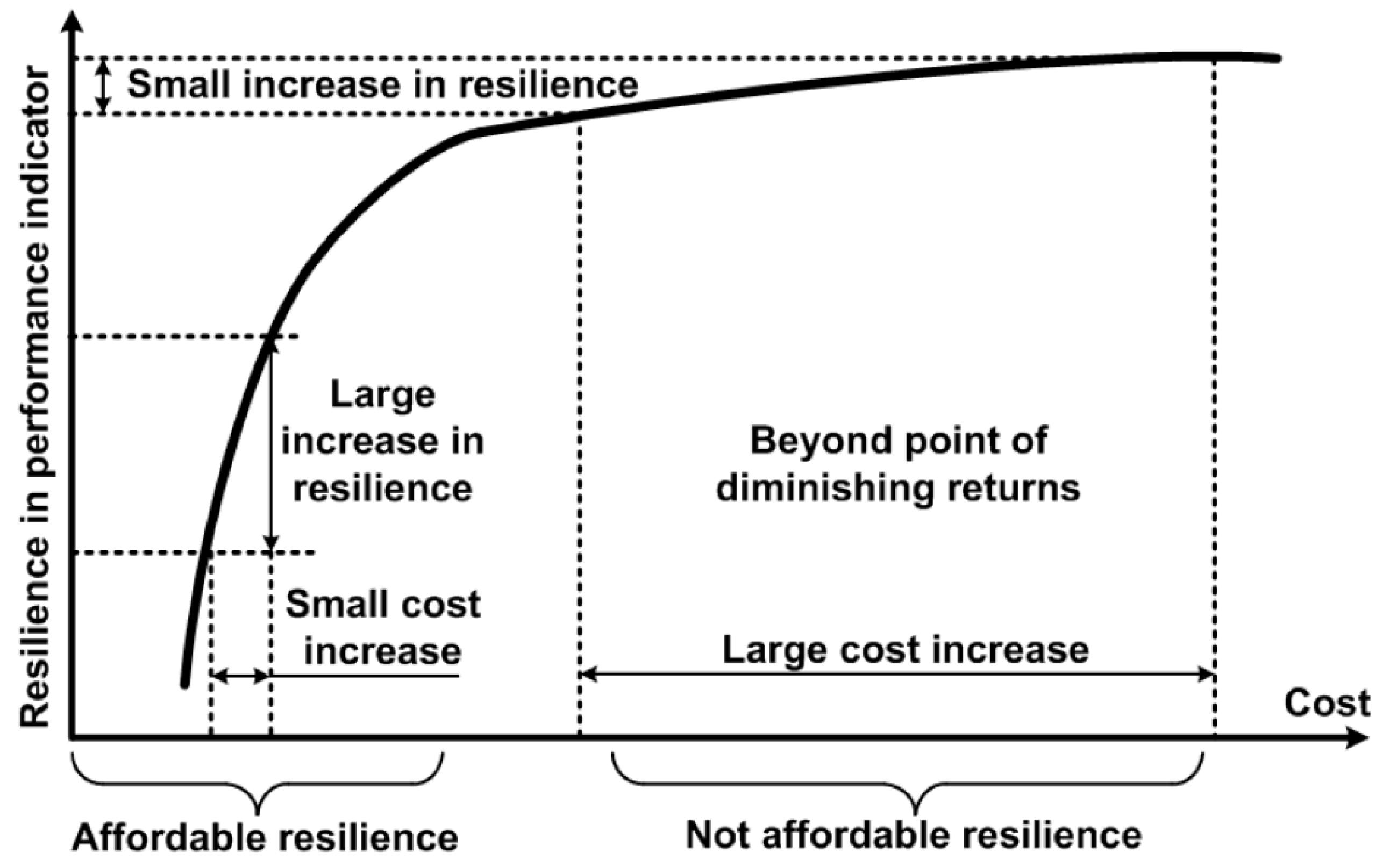
Figure 2. Cost curve for ensuring system resilience.
Preprints 68606 g002
Figure 4. Propagation of hardware failure from the physical layer of the computing environment to the behavioral layer of the neural network application.
Preprints 68606 g004
Figure 6. Diagram of the methodology for adaptive fault and error injection into a digital device on which a AI-model is deployed.
Preprints 68606 g006
Figure 8. Taxonomy of AIS resilience.
Preprints 68606 g008
Figure 9. The ontological diagram of AIS resilience.
Preprints 68606 g009
Figure 10. Illustration of the resilience curve and its key indicators.
Preprints 68606 g010
Figure 11. Functional diagram of AIS resilience testing.
Preprints 68606 g011
Figure 13. Illustration of alternative intervals for testing the Chernoff bounds.
Preprints 68606 g013
Table 1. Approaches and algorithms to ensure the recognition and absorption of adversarial attacks.
Approach Capability Weakness Methods and Algorithms
Gradient masking Perturbation absorption Vulnerability to attacks based on gradient approximation or black-box optimization with evolution strategies Non-differentiable input transformation [50,51]
Defensive distillation [52]
Models selection from a family of models [53]
Generative model PixelDefend or Defense-GAN [54,55]
Robustness optimization Perturbation absorption and performance recovery Significant computational resource consumption to obtain a good result Adversarial retraining [65]
Stability training [57]
Jacobian regularization [58]
Sparse coding-based representation [60]
Intra-concentration and inter-separability regularization [30,31,59]
Provable defenses with the Reluplex algorithm [65]
Detecting adversarial examples Rejection Option in the presence of adversarial inputs with the subsequent AI-decision explanation and passing the control to a human Not reliable enough Light-weight Bayesian refinement [61]
Adversarial example detection using latent neighborhood graph [62]
Feature distance space analysis [67]
Training Data Sanitization algorithms based on Reject on Negative Impact approach [63]
Table 2. Approaches and algorithms of faults detection and absorption.
Approach Capability Weakness Methods and Algorithms
Fault masking Perturbation absorption Computational intensive model synthesis Weights representation with error-correcting codes [68]
Neural architecture search [69]
Fault-tolerant training based on fault injection to weight or adding noise to gradients during training [70]
Explicit redundancy Perturbation detection and absorption Computationally intensive model synthesis and inference redundancy overhead Duplication of critical neurons and synapses [71]
Multi-versioning framework for constructing ensembles [72]
Error correcting output coding framework for constructing ensembles [73]
Error detection Rejection Option in the presence of neural weight errors with the subsequent recovery by downloading a clean copy of weights The model does not improve itself and information from vulnerable weights is not spread among other neurons Encoding the most vulnerable model weights using a low-collision hash-function [74]
Checksum-based algorithm that computes low-dimensional binary signature for each weight group [75]
Сomparision contrastive loss function value for diagnostic data with the reference value [76]
Table 3. Approaches and algorithms of drift detection and mitigating.
Approach Capability Weakness Methods and Algorithms
Out-of-domain generalization Absorption
of disturbance
Less useful for real concept drift Domain randomization [78]
Adversarial data augmentation [79]
Domain-invariant representation [80]
Heterogeneous-domain knowledge propagation [81]
Ensemble selection Absorption
of disturbance
Not suitable for large deep neural networks and high-dimensional data Dynamically weighted Ensemble [82]
Feature dropping [83]
Concept Drift detection Rejection Option in the presence of Concept drift with the subsequent adaptation Not reliable when exposed to noise, adversarial attacks or faults Data distribution-based detection [84]
Performance-based detection [85]
Multiple hypothesis-based detection [86]
Contextual-based detection [87,88]
Out-of-distribution detection Rejection Option in the presence of out-of-distribution data with the subsequent passing the control to a human and
active learning
Expensive calibration process to obtain a good result Data and training based epistemic uncertainties estimation [89]
Model-based epistemic uncertainties estimation [90]
Post-hoc epistemic uncertainties estimation [91]
Table 5. Approaches and algorithms to ensure the adaptation and evolution.
Approach Capability Weakness Methods and Algorithms
Active learning, continual learning
and lifelong learning
Might update the AIS knowledge about data distribution (active learning case), or begin to give the AIS knowledge about new task (continual / lifelong learning case). Low-confidence samples should be continuously labelled by the oracle (operator) manual intervention typically is expensive.
It is necessary to adjust settings to combat catastrophic forgetting problems.
Active learning with Stream-based sampling [103]
Active learning with Pool-based sampling [104]
Regularization-based continual learning [105]
Memory-based continual learning [106]
Model-based continual learning [107]
Domain Adaptation Effective in overcoming the difficulty of passing between domains when the target domain lacks labelled data.
Can be used in heterogenous setting, where the task is changing as opposed to the domain.
Such methods can be intensive during the training phase and will require large amounts of computational resources.
Quick adaptation might not be achievable in this paradigm.
Discrepancy-based Domain Adaptation [108]
Adversarial Domain Adaptation [109]
Reconstruction-based Domain Adaptation [110]
Self-supervised Domain Adaptation [111]
Meta-learning These methods are effective in creating effective and adaptive models.
Stand out applications
include fast, continual, active, and few-shot learning, domain generalisation, and adversarial defence.
Meta-learning models can be very resource-intensive to instantiate, due to the necessity to train on large amounts of data.
Memory-based methods [112]
Gradient-based methods [113]
Unified (combined) methods [114]
Table 6. Approaches and algorithms addressed to loss-metric mismatch issue.
Approach Capability Weakness Examples of method or algorithm
Surrogate losses Obtained loss function is better aligned to metric These hand-designed losses not only require tedious manual effort and white-box metric formulation, but also tend to be specific to a given metric. Batching Soft IoU for Semantic Segmentation [133]
Hinge-rank-loss as approximation of Area under the ROC Curve [134]
Сonvex Lovasz extension of sub-modular losses [135]
Strongly proper composite losses [136]
Trainable surrogate losses Removed the manual effort to design metric-approximating losses. Loss learning based on metric relaxation schemes instead of a direct metric optimization. Stochastic Loss Function [137]
Loss combination techniques [138]
Direct metric optimization
with true metric embedding
Providing of correction term for metric optimization. Their common limitation is that they require the evaluation metric to be available in closed-form. Plug-in classifiers for non-decomposable performance measures [139]
Consistent binary classification with generalized performance metrics [140]
Optimizing black-box metrics with adaptive surrogates [141]
A unified framework of surrogate loss by refactoring and interpolation [142]
Black-box evaluation metrics optimization using a differentiable value function Directly modeling of black-box metrics which can in turn adapt the optimization process. There is a need to change the AI-model by introducing conditional parameters.
The learning algorithm is complicated by metric meta-learning and meta-testing
Learning to Optimize Black-Box Evaluation Metrics [143]
Disclaimer/Publisher’s Note: The statements, opinions and data contained in all publications are solely those of the individual author(s) and contributor(s) and not of MDPI and/or the editor(s). MDPI and/or the editor(s) disclaim responsibility for any injury to people or property resulting from any ideas, methods, instructions or products referred to in the content.
Copyright: This open access article is published under a Creative Commons CC BY 4.0 license, which permit the free download, distribution, and reuse, provided that the author and preprint are cited in any reuse.
Prerpints.org logo

Preprints.org is a free preprint server supported by MDPI in Basel, Switzerland.

Subscribe

© 2024 MDPI (Basel, Switzerland) unless otherwise stated