1. Introduction
Face stability is critical in shallow tunnels to avoid collapse. In mechanised tunnels, the face support is provided by the tunnel boring machine (TBM), e.g. slurry (SPB) or earth pressure balance (EPB) shields. An estimate of the support pressure is required for safe and efficient construction.
The problem of face stability can be solved with analytical, numerical and experimental approaches. The analytical methods are mainly based on the limit state analysis [
1,
2,
3,
4,
5,
6,
7,
8,
9]. Face stability can also be investigated by numerical analysis [
10,
11,
12,
13,
14,
15,
16,
17]. Alternatively, the problem can be studied experimentally at 1g [
13,
14,
18,
19,
20,
21] or with centrifuge model tests [
22,
23,
24].
Recently, machine learning has emerged as a promising technique for predictive assessment in geotechnical engineering, in general [
25,
26,
27,
28,
29,
30,
31], and in tunnelling, in particular [
32,
33,
34,
35,
36,
37,
38]. Some promising research domains for machine learning in tunnelling are the geological prognosis ahead of the face, the interpretation of monitoring results, automation and maintenance [
32]. At present, however, research appears to be focussed on the following topics: prediction of TBM operational parameters [
34,
39,
40,
41,
42,
43,
44,
45,
46], penetration rate [
47,
48,
49,
50,
51,
52,
53,
54,
55,
56,
57,
58,
59,
60,
61,
62,
63], pore-water pressure [
64], ground settlement [
65,
66,
67], disc cutter replacement [
68,
69,
70], jamming risk [
71,
72] and geological classification [
73,
74,
75,
76]). Few authors estimated the face support pressure of TBMs with machine learning [
35,
52].
The previous studies developed models that are trained after tunnel construction and thus pertain to the domain of supervised learning, the machine learning paradigm where the predictions are based on labelled datasets [
77]. This study proposes a method to determine the face support pressure of TBMs with reinforcement learning. Within the realm of artificial intelligence, reinforcement learning is a generic framework for representing and solving control tasks in which the actions performed by the algorithm at one time are influenced by past decisions. Reinforcement learning algorithms are trained by incentivising them to accomplish a goal. Although reinforcement learning research is still in its infancy, there have been recently some exciting developments, most notably those showcased by the Google’s DeepMind research group [
78,
79,
80,
81,
82], which demonstrated the ability to master Atari video games and popular board games such as chess and go. The transition of reinforcement learning from academia to industry is gaining momentum. Noteworthy examples are dynamic job shop scheduling [
83], memory control optimisation [
84,
85], personalised web services [
86,
87], self-driving cars [
88], algorithmic trading [
89], natural language summaries [
90] and healthcare applications such as dynamic treatment regimes and automated medical diagnosis [
91]. Reinforcement learning industrial products include Google Translate, Apple’s Siri and Bing Voice Search [
92].
Unfortunately, only few such studies are found in geotechnical engineering, especially in tunnelling. In particular, Erharter and Marcher presented a framework for the application of reinforcement learning to NATM tunnelling in rock [
93] and to the TBM disc cutter replacement [
68]. Zhang et al. [
94] employed reinforcement learning to predict tunneling-induced ground response in real time.
In this study, the capability of the reinforcement learning algorithm to choose the best sequence of face support pressures is investigated by adapting the algorithm used by the DeepMind research group [
80] and testing it on random geologies. The novelty of our method resides in the reinforcement learning approach, where the machine has no previous knowledge of the environment which it explores and is educated through the rewards defined by the user, as well as in the simulation of the environment with the finite difference method (FDM). This study shows that our model is capable of optimising the face support pressure, provided that a sufficient number of episodes are played.
In the following, the proposed method is presented (
Section 2). The method is tested in environments of growing complexity, from analytical calculations to numerical analysis (
Section 3). Its performance, limitations and possible improvements are discussed in
Section 4. Finally,
Section 5 concludes the paper.
2. Methods
In this section, the reinforcement learning algorithm is described. It is implemented with the interpreted high-level general-purpose programming language Python [
95]. The algorithm is tested against analytical calculations (
Section 2.1) and numerical analysis (
Section 3.4).
One of three basic machine learning paradigms alongside supervised and unsupervised learning, reinforcement learning involves learning optimal actions that maximize a numerical reward [
96]. In other words, reinforcement learning deals with the way (the policy) an intelligent agent (an algorithm) takes the actions that maximise a user-defined reward in a particular setting (the state of the environment).
The policy defines how the algorithm behaves in a certain situation. More precisely, it connects the states of the environment to the actions to be taken. As such, the policy is the core of a reinforcement learning agent, given that it determines its behaviour [
96]. The well-established “epsilon greedy strategy”, one of the oldest policies [
96], is selected in this study. An action is considered “greedy” if it is expected to return the maximum reward for a given state. However, since the environment is unknown
a priori, an initial exploration of the environment is necessary to determine these actions. This exploration begins with the first TBM excavation where the face support pressure is randomly chosen at every round. The randomness decreases after every episode as the environment knowledge is exploited.
At each excavation round
i, the agent chooses a random action
with probability
and the action associated with the highest expected reward
with probability
.
is initialised at 1, which corresponds to a completely random selection, and decremented by
after each episode, where
N is the total number of excavations (the episodes). For
N episodes,
decreases by
per episode until it reaches 0. In mathematical terms, let
be a random number and
at episode
j, the agent takes the action
at the state
i according to equation (
1), where
is a random integer.
Hence, the random choice of the face support pressure is initially the dominant pattern that is slowly, but steadily, abandoned over time as the agent gains some experience of the environment in which it operates. In other words, the face support pressure becomes more of a “conscious” choice based on the rewards collected and represented by the value function , which returns the reward expected for the action a in the state s.
The rewards are user-defined and determined by the support pressure, the excavation rounds and the surface settlement. They reflect the definition of efficient construction: a safe process (consisting in the minimisation of surface settlement) executed with the least possible effort (determined by the lowest possible support pressure). The actual reward values are irrelevant, as long as the algorithm can maximise the expected reward, given the input data. The relative weight of the rewards, however, has an impact on the results [
97].
A
reward is collected at each excavation round. The lower the face support pressure applied by the TBM, the lower the building effort. Hence, a reward corresponding to
is assigned to every action. The surface settlement at every round causes a
reward for each mm of additional settlement. A
reward is assigned if the surface settlement is larger than 10 cm (in the analytical environment) or if the calculations diverges (in the finite difference environment). These outcomes terminate the episode (game over). A
reward is assigned at excavation completion. Each completed or terminated tunnel excavation defines an episode. The rewards are listed in
Table 1.
The “playground” of the agent is named environment [
98]. The actions are chosen and the rewards are received by the agent in the environment. In the present case, two classes of environments are created. First, an environment consisting of simple analytical calculations of the required face support pressure and expected settlements is considered (
Section 2.1). The second environment is simulated numerically via the FDM as described in
Section 3.4.
2.1. Analytical training environment
In the following, the initial training environment of the algorithm is described. For a tunnel with diameter
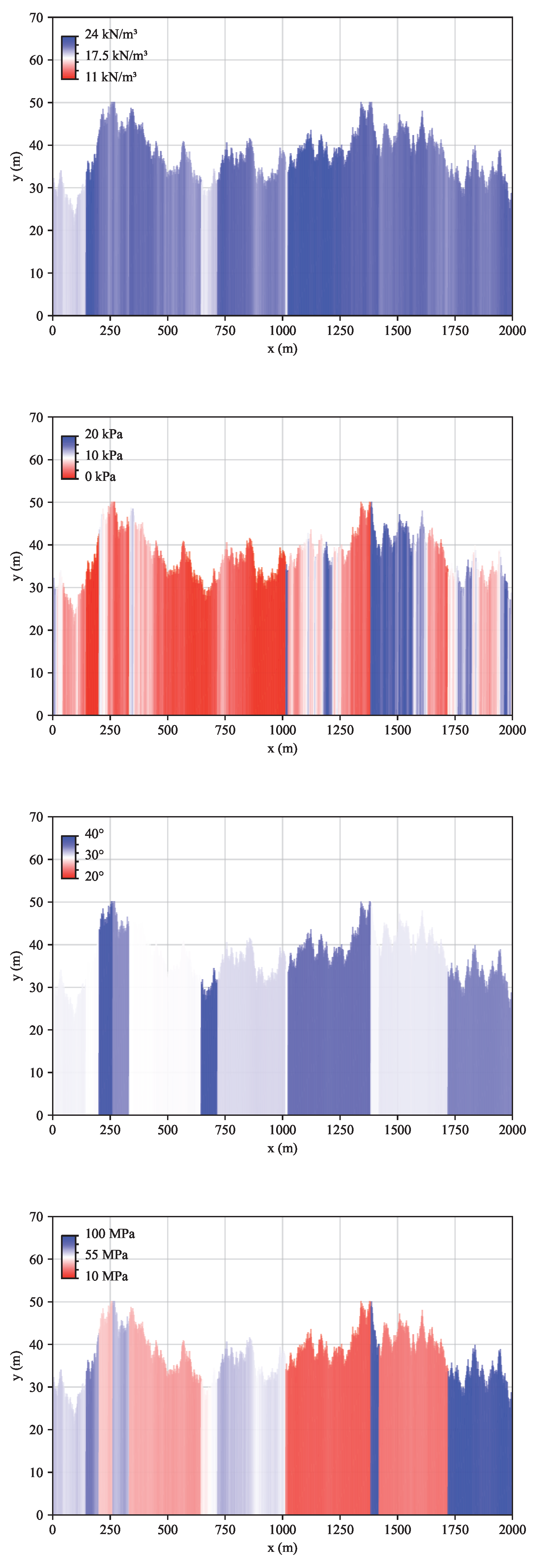
m, a random 2000 m long geological profile is generated (
Figure 1). The pseudorandom number generator is initialised with a constant seed so that the results can be replicated. The 2000 m length corresponds to the break-even point for the choice of mechanised over NATM tunnelling [
99]. At first, this geology is kept constant and is thus the same for all the 100 training episodes. In the second instance, different random geological profiles are created at each episode (
Section 3.2). The soil cover
C is randomly initialised in the interval
. The soil cover to diameter ratio is capped at
. At every 2 m (the excavation step or round length), a random slope is selected from the interval
, corresponding to the interval of slope angles
. The soil unit weight
, friction angle
, cohesion
c and Young’s modulus
E are randomly initialised in the intervals shown in
Table 2. The soil property values slightly change from their initial values at every excavation step (
Table 1). The soil properties are re-initialised with a
probability at every 2 m to simulate soil stratification.
By moving across states of these environments, the agent collects the rewards and stores them in the so-called value function . The state representation is described in the next section.
2.2. State representation
The state is a representation of the information necessary and relevant to take an action. It is not the physical state of the environment, but rather a representation of the information for the algorithmic decision-making [
100].
Since there are no rules to determine the state variables, domain knowledge, i.e. “the knowledge about the environment in which the data is processed” [
101], must be used. According to the literature [
4,
7,
12,
16,
22], face stability primarily depends on the soil unit weight, cohesion, friction angle and the depth of the overburden. Furthermore, soil settlement depends on the soil Young’s modulus
E and the stress release [
102]. Hence, the soil properties
,
c,
,
E directly ahead of the tunnel face and the overburden
C are normalised by dividing them by their maxima
,
,
,
,
(
Table 2) and selected as the state variables. The stress release is determined by the choice of the support pressure.
Generally, TBMs cannot estimate the soil properties ahead of the tunnel face [
103]. However, boreholes are retrieved prior to soil excavation and analysed in the laboratory to obtain the material properties for the engineering design. Unfortunately, due to the soil heterogeneity, the property values cannot perfectly match reality, but are rather mean values that can be nonetheless used as a first approximation.
2.3. Face support pressure and settlement
TBMs provide face support pressures up to approximately 200 to 300 kPa in soft soils [
104]. At every excavation step, the proposed model searches the optimal support pressure within the interval
kPa. According to the guidelines [
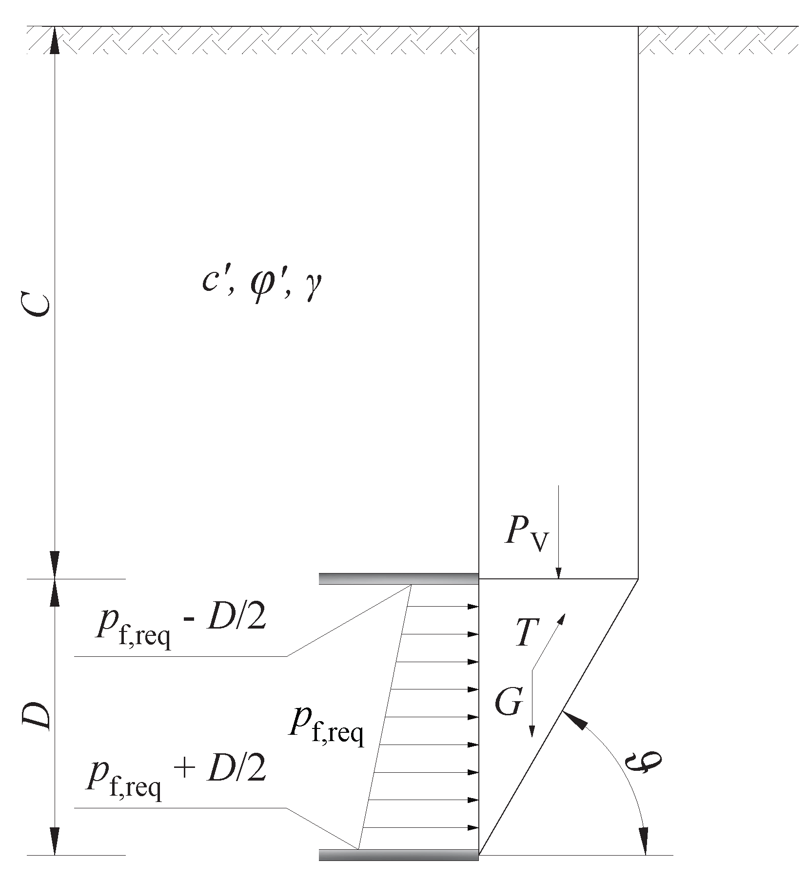
4], based on a limit equilibrium approach for drained conditions, the required support pressure is calculated with
where
is the cross-sectional area of the tunnel,
G is the self weight of the sliding wedge,
is the vertical load from the soil prism, and
T is the shear force on the vertical slip surface (
Figure 2). The critical value of the sliding angle
that maximises
is searched iteratively with the Python package
scipy [
105]. Note that the guidelines differentiate between
and
above the tunnel tunnel and
and
at the level of the tunnel. In this simulation, however,
and
.
The proposed model estimates the support pressure
at every step to maximise the expected outcome according to the following criteria and compares it with the required pressure
. In this simplified environment, the surface settlement occurs if
and the stress release
is calculated as the ratio of the provided to the required tunnel face support pressure, so that
. The corresponding soil settlement is then calculated as follows [
102].
In reality, the settlement occurs not only due to the stress release at the tunnel face, but also due to other factors, such as the overcutting and ring gap [
102]. Furthermore, an experience factor
depending on ground stress and conditions, and tunnel geometry is generally considered in equation
3.
Since the model has no prior information about the required support pressure , the support pressure is chosen randomly during the first episode. Then, the model learns the optimal support pressure based on the rewards collected, as explained in the next section.
2.4. Deep Q-Network
In this section, the algorithm to maximise the rewards collected during the TBM excavation is elucidated. Since the material properties have continuous values, the number of possible states as described in
Section 2.2 is infinite. Hence, the model cannot have a complete knowledge of the expected reward associated with the actions at each state and the knowledge of the value function
is thus incomplete. This is where the Deep Q-Network (DQN) comes into play.
The DQN uses deep neural networks to approximate the value function
[
106]. This algorithm was developed by DeepMind, the Google research group, and was able to play six Atari games at record levels [
78,
80,
81,
82,
107]. DQN is a particular approach to Q-learning, a method of learning optimal action values, whose main idea is to predict the value of a state-action pair, compare this prediction to the observed rewards and update the parameters of the algorithm to improve future predictions. Q-learning algorithms are formally described by equation (
4).
In the present example, the DQN is trained to choose the best tunnel face support pressure based on the state variables. The DQN receives the state vector as the input and delivers the vector of the expected rewards associated with every action as the output. After the action is taken and the agent moves to the new state , the reward is observed. The algorithm is run again with as the input and returns the action with the highest value . Finally, the learning algorithm is updated to reflect the actual reward, using the mean squared error as loss function and minimising the difference between the predicted and target prediction of .
In equation (
4),
and
are the hyperparameters that influence the algorithm learning process.
is the learning rate. The algorithm makes only small updates at each step with a low value of
and large ones with a high value. The hyperparameter
is the discount factor and controls how much our agent discounts future rewards when making a decision. Given that the discount factor is less than 1 (
Table 3), future rewards are discounted more than immediate rewards.
The deep neural network is implemented using the
PyTorch library [
108] of the Facebook AI Research lab and its higher-level interface
nn, as explained in [
109].
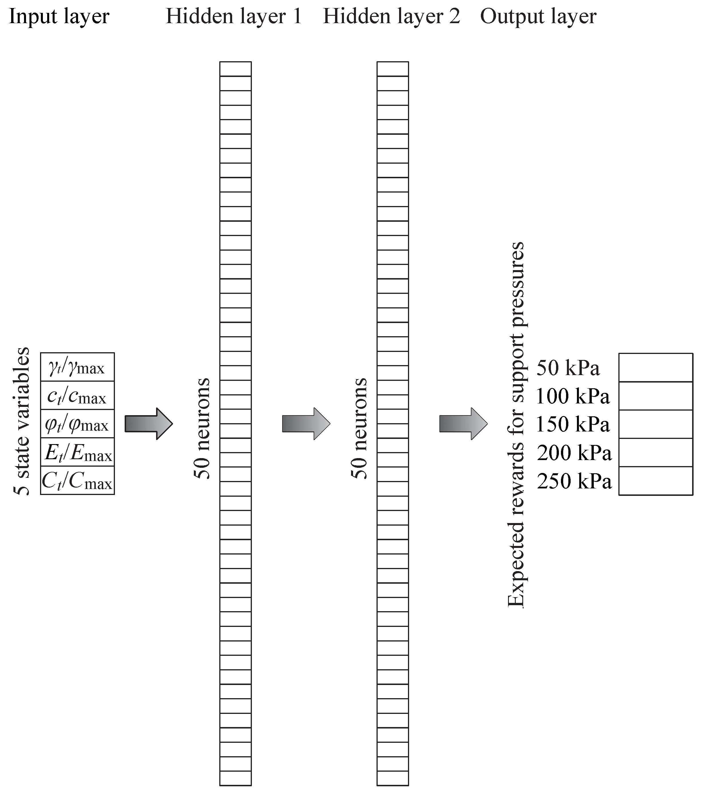
Figure 3 shows the architecture of the neural network. The input layer is the state vector whose elements are
,
,
,
and
. The support pressure
is comprised in the discrete interval of natural integers
kPa and is assigned in 50 kPa steps. Hence, the output layer is a vector with five elements, one for each possible support pressure (50, 100, 150, 200 and 250 kPa). The first and second hidden layers have each 50 neurons. This architecture has been previously applied to slope stability and tunnelling [
36,
110] and is the result of a trade-off between learning capabilities and computational effort.
However, DQNs are generally prone to training instability [
78]. Hence, the following sections describe two common techniques used to stabilise the DQN, namely experience replay [
111] and target memory [
78].
2.4.1. Experience replay
Since the soil properties are variable in nature, the algorithm cannot simply memorize a sequence of support pressures . It must find the maximum support pressure that cause little to no surface settlement regardless of the geological setting.
However, reinforcement learning is essentially a trial-and-error process, which could lead to unstable solutions. This instability is particularly evident if learning is slow, which occurs when the rewards are sparse. This problem is deemed “catastrophic forgetting” [
112] and is a common issue of gradient descent-based training methods in online training, i.e. when backpropagation is performed after each state. The essence of catastrophic forgetting is the push-pull between very similar state-action pairs that results in the inability to train the algorithm.
To this end, experience replay can be used to accelerate the learning process [
111] by adding batch updating to the online learning scheme, as follows:
In state i, the algorithm takes action a, and observes the new state and reward ,
it stores this as a tuple in a list and
continues to store each experience until the list is filled to a specific length, called “memory size” ().
Once the experience replay memory is filled, a subset with a predefined batch size () is randomly selected.
The algorithm iterates through this subset and calculates the value updates for each subset; it stores these in the target array Y and the state s of each memory in X.
Finally, it uses X and Y as a mini-batch for training and overwrites the old values in the experience replay memory when the array is full.
Thus, in addition to learning the value of the actions, a random sample of past experiences is also used for training. A further refinement is represented by the target memory.
2.4.2. Target memory
In DQNs, instabilities can arise by updating the parameters after each action. This instability is caused,
inter alia, by the correlation between subsequent observations and can be overcome by updating the value function
only after a prescribed number of episodes [
78].
In the present problem, the rewards are “sparse”, i.e. they are significantly higher at the end of each episode than after every action. To solve this problem, the Q-network is duplicated. The parameters of this copy, i.e. the target
-network, are not up-to-date and lag behind the regular Q-network [
78]. The
-network is implemented as follows:
The Q-network is initialised with parameters and
the -network is a copy of the Q-network with distinct parameters . At first, .
The epsilon-greedy strategy is used with the Q-values of the Q-network to select the action a.
The reward and new state and are observed.
The -values of the -network are set to at the end of the episode or to otherwise.
The -value is backpropagated through the Q-network (not the -network).
After a certain number of iterations, called synchronisation frequency (f), is again set equal to .
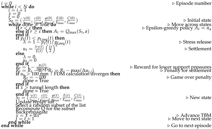
Up to this point, all the features of the algorithm 1 have been presented. In the next section, the results of the analytical environment are presented. The values of the hyperparameters
,
,
f,
and
are chosen based on the sensitivity analysis of
Section 3.1.
|
Algorithm 1:Workflow of the Reinforcement Learning algorithm |
 |
3. Results of the analytical environment
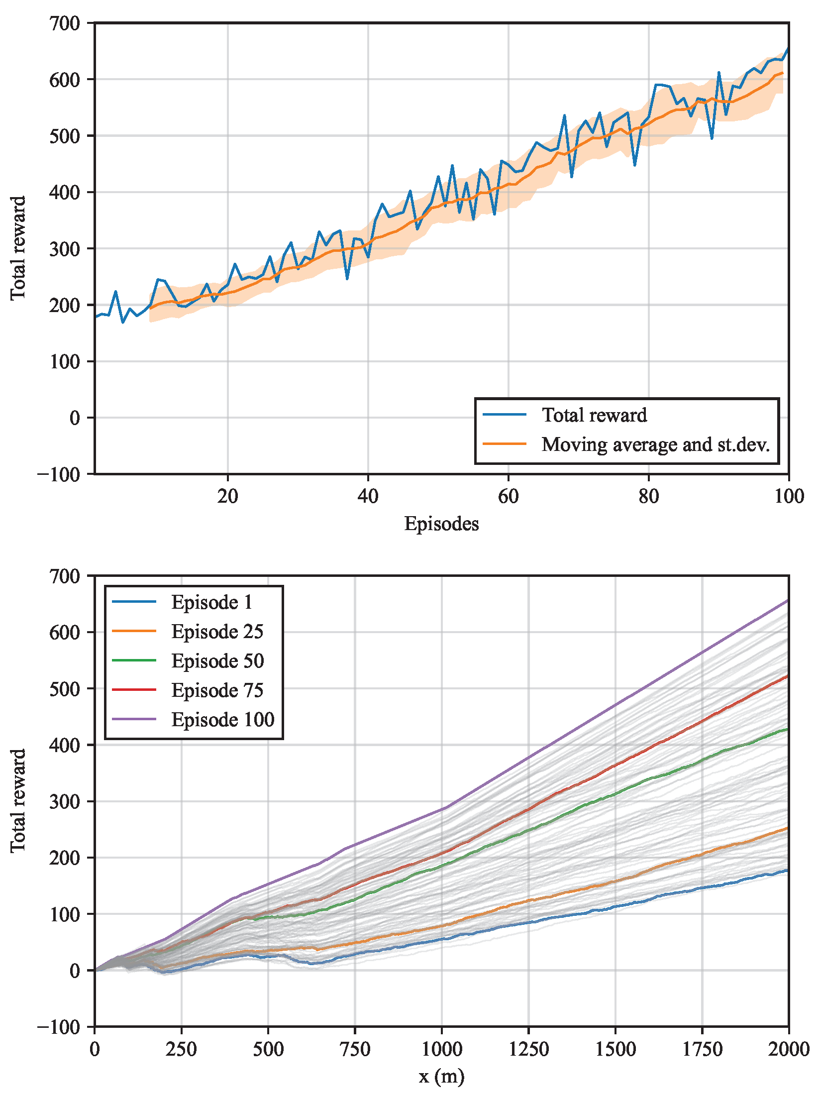
In this section, the results of the analytical environment are presented. The cumulative reward collected at every episode is shown in
Figure 4a. The orange line represents the moving average of 10 episodes and the orange band is the range of
standard deviations. Since the algorithm is trained on the geology of
Figure 1 only, the reward increases steadily, barely oscillating around the moving average. In
Figure 4b, the cumulative rewards obtained from the
,
,
and
episodes are highlighted. As expected, the reward increases more rapidly for the last episodes. Also, approximately at the “chainages”
and 700 m, slight drops in the cumulative reward occur due to the abrupt changes in geology (
Figure 1).
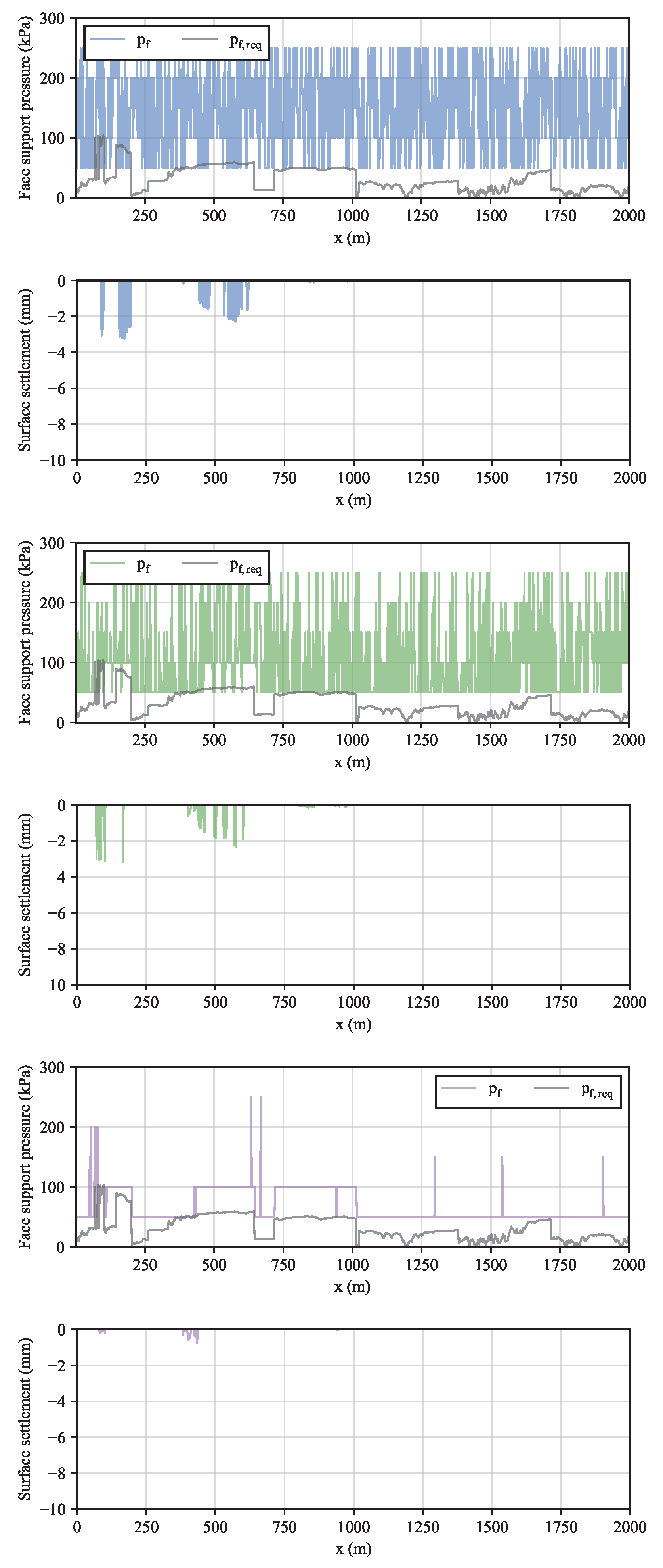
The support pressures and the resulting settlement at the episodes 1, 50 and 100 are shown at the left side and right sides of
Figure 5, respectively. As the support pressure is randomly chosen at the first episode,
Figure 5a exhibits a chaotic behaviour. As the agent learns the optimal support pressures, this behaviour is mitigated and the support pressure becomes more stable (
Figure 5c).
Figure 5c also proves that the algorithm is able to choose the support pressure in such a way that it almost encases the required pressure. Furthermore, even when
, the resulting settlement is negligible (
Figure 5f). The model sensitivity to changes in the values of the hyparameters is studied in the next section.
3.1. Sensitivity analysis
Contrary to the parameters of the deep neural networks depicted in
Figure 3 that are learnt by the algorithm, hyperparameters are set by the user. In
Section 2, a number of hyperparameters have been introduced, such as the discount factor
, learning rate
, synchronisation frequency
f, the memory
and batch
sizes.
The model sensitivity to these hyparameters is summarised in
Table 3. Obviously, the results are not very sensitive to the discount factor and
returns the highest cumulative reward. A low value of
implies that the action taken at one state has little impact on the actions taken in the following states. This seems plausible for tunnelling where the settlement caused by an excessively low support pressure cannot be possibly offset by a later support pressure increase. The optimal learning rate is a matter of numerical stability. In this study,
appears to be the optimal value and, if the learning rate is set at
, the cumulative reward cannot be properly maximised. The cumulative reward is not very sensitive to the synchronisation frequency where the optimal value is 5 episodes. The memory size has a more pronounced effect and the optimal value is 10. Finally, the batch size of 2 episodes provides the best results.
In summary, the proposed model is not very sensitive to the discount factor and the synchronisation frequency, it is starkly affected by the learning rate and the memory size in this particular problem. After the hyperparameters are optimised, the algorithm is tested against random geologies in the next section.
3.2. Random geologies
Prompted by the initial success in optimising the cumulative reward with constant geology, the algorithm is further tested against random geologies. Hence, the depth of the overburden and the material properties are no longer fixed as depicted in
Figure 1, but change at every episode.
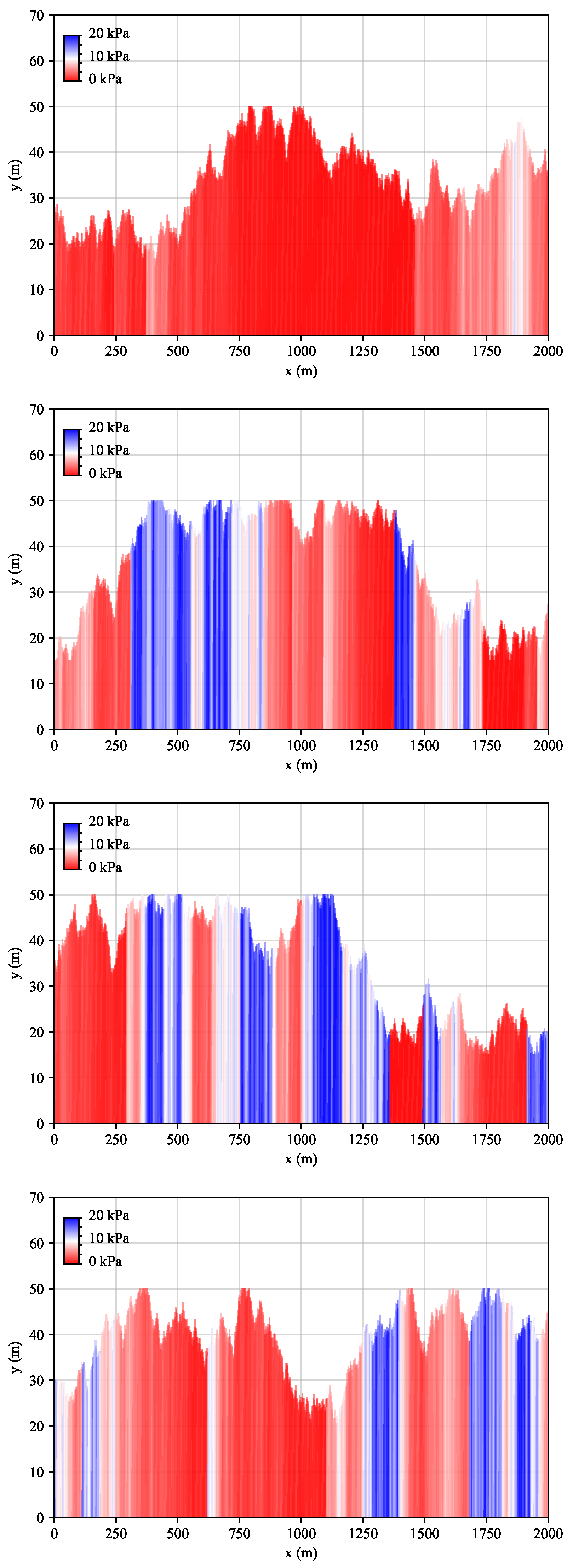
Figure 6 exemplarily shows the profiles of the cohesion values at the episodes 2, 3, 4 and 5.
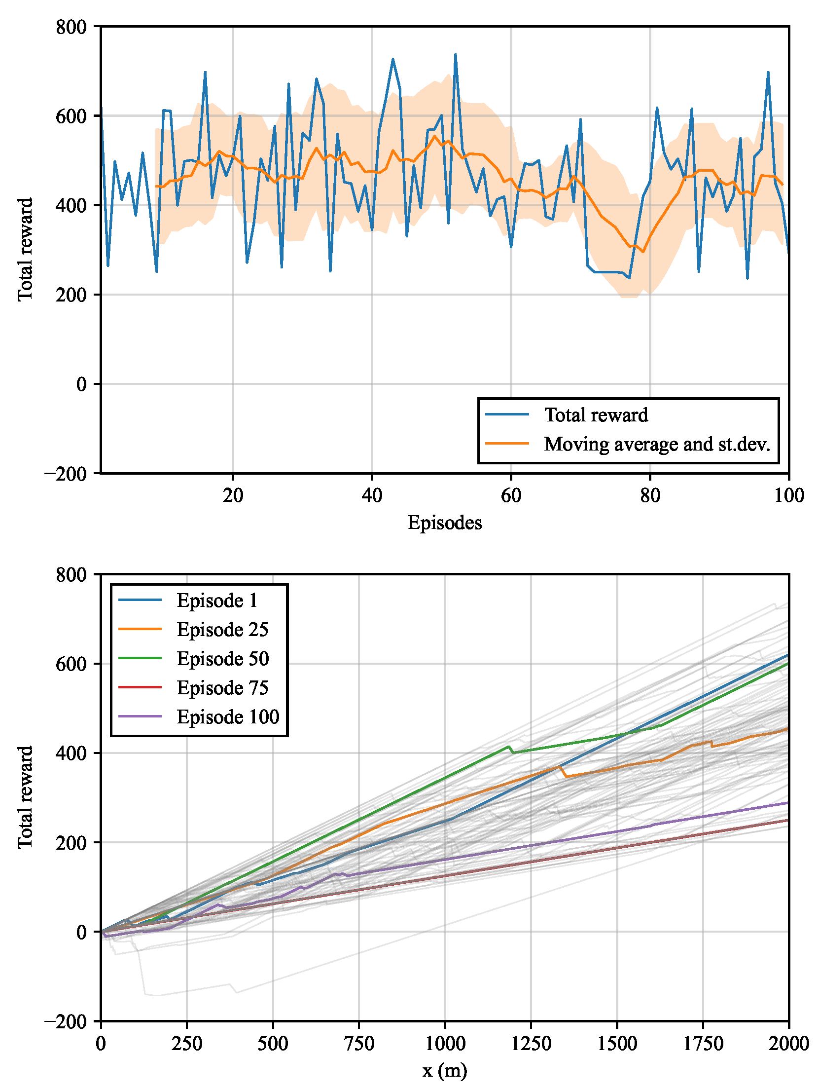
Clearly, since the environment changes at every episode, the cumulative reward shown in
Figure 7a does not increase steadily as in
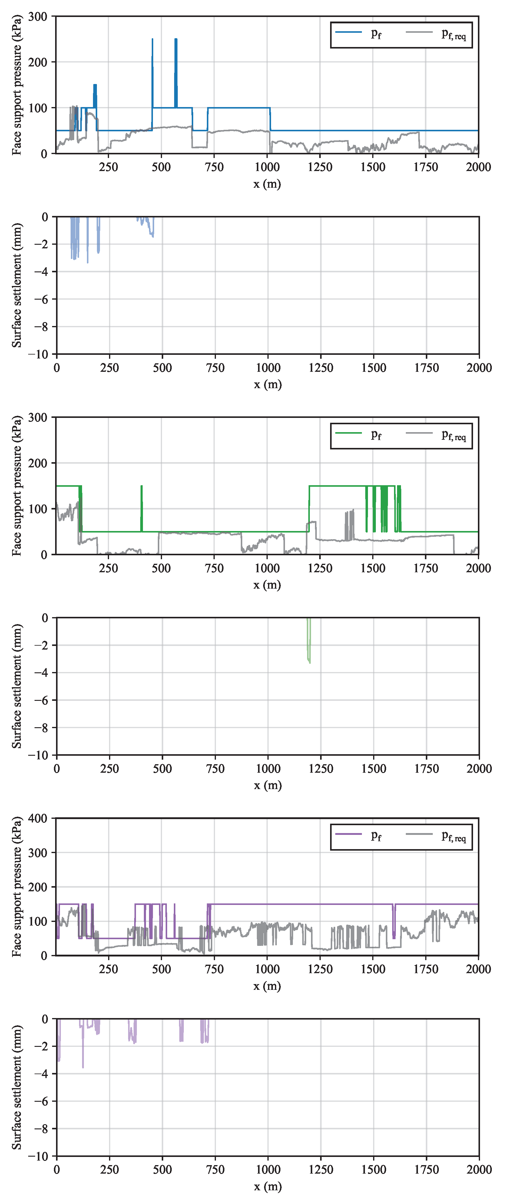
Figure 4a, but swings markedly. The model is able to forecast the support pressure increases to accommodate for larger
in different settings (
Figure 8). Furthermore, even when the support pressure provided fall below the required one, the resulting settlement is lower than about 4 mm.
The previous results are obtained with no additional model training. This means that the initial value of
is set to zero. By starting from different values of
, it is shown in the following that no additional exploration is needed. Note that, strictly speaking, even if
the Q-value is slightly updated as rewards are collected along the way. The agent, however, would perform the same action, given a certain state, until its expected rewards falls below that of other actions. The results of this analysis are shown in
Table 4 where the mean cumulative reward and standard deviation are listed for different
. The highest mean cumulative reward and the lowest standard deviation are achieved for
. Therefore
is selected as the optimum value, meaning that no additional exploration is required to optimise the algorithm performance in the random analytical environment. The numerical environment is described in the next section.
3.3. Effect of the Number of Episodes
When more episodes are played, the environment is explored more thoroughly. Hence, it is expected that the maximum cumulative reward increases with the number of episodes.
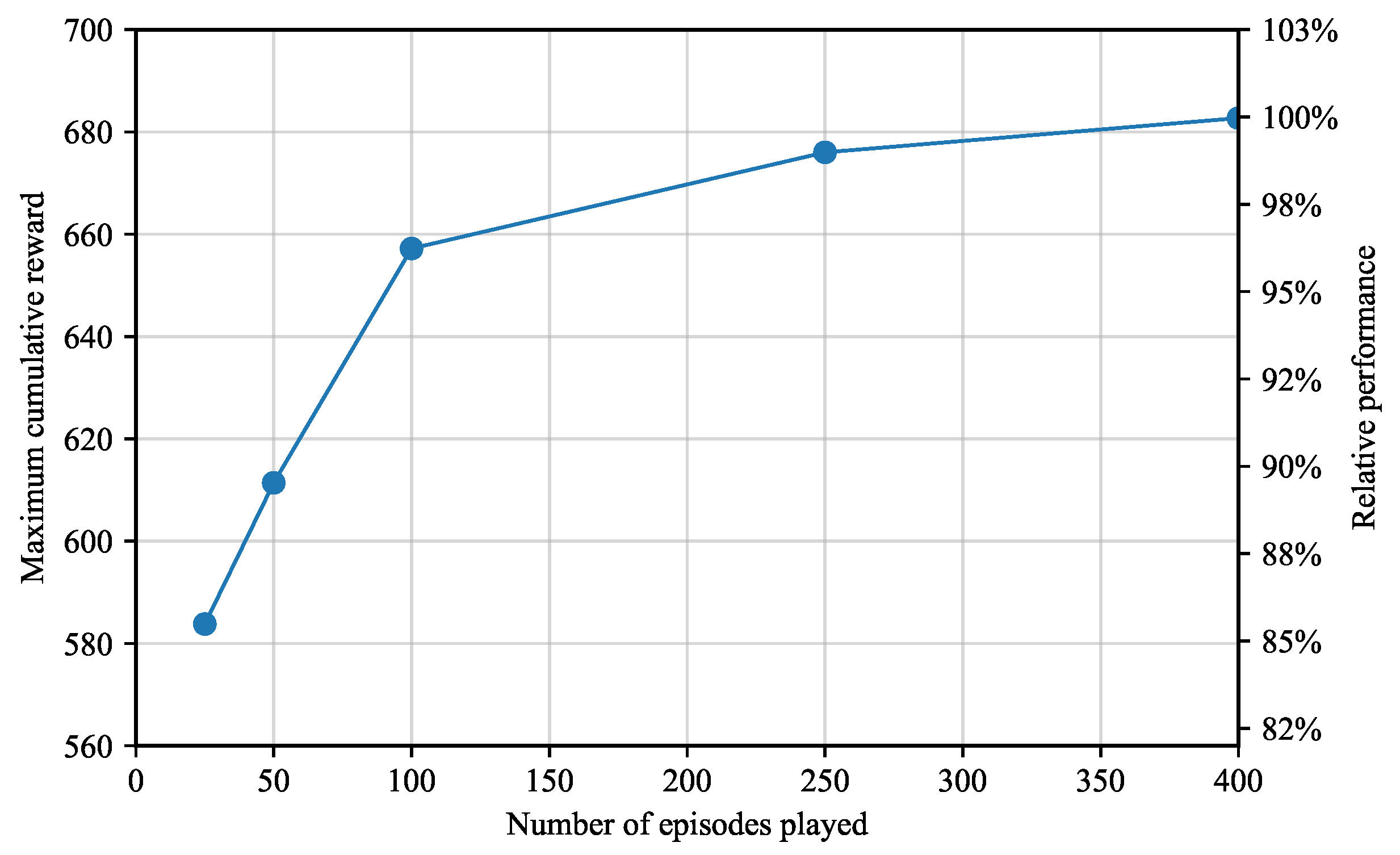
Figure 9 shows that the maximum cumulative reward grows asymptotically up to approximately 683 after 400 episodes. It also shows that, the maximum cumulative reward obtained after 50 episodes already represents approximately 90% of the maximum reward achieved after 400 episodes.
3.4. Finite Difference Environment
Due to the simplified analytical formulations, the previous environment is not very realistic. It is, however, useful to demonstrate the capability of the model and to optimise its hyperparameters. Tunnels are often simulated with numerical analysis [
113,
114,
115,
116]. Hence, a more realistic finite difference environment is outlined in the following based on the finite-difference program FLAC
3D [
117].
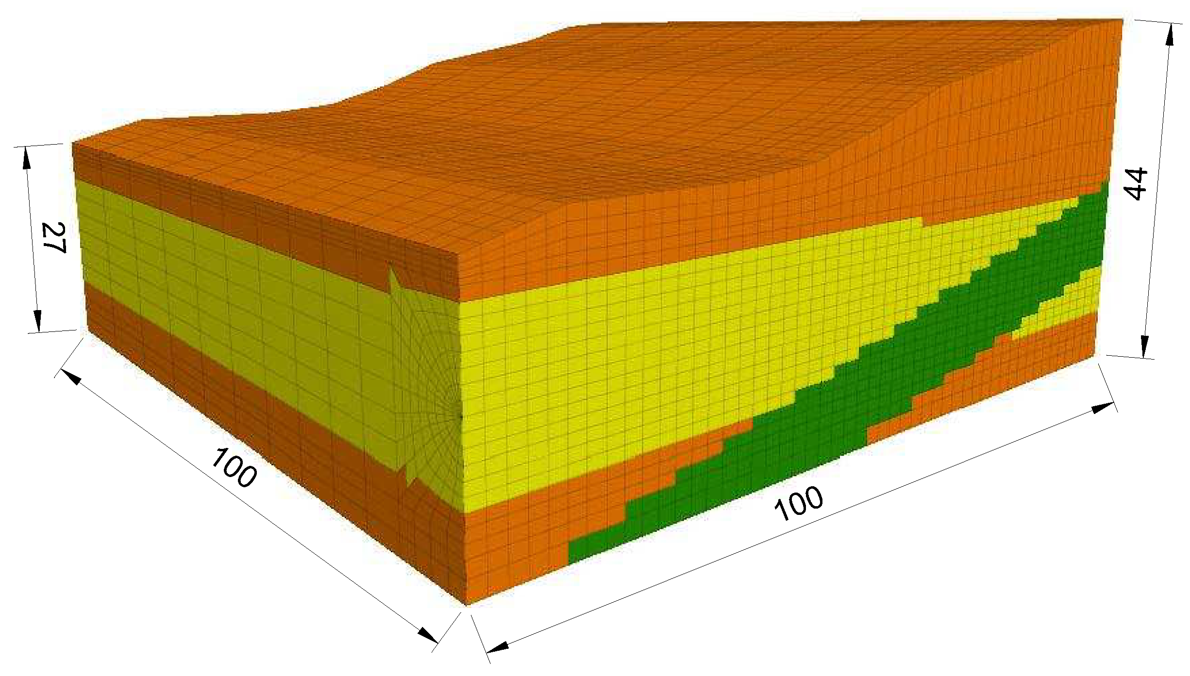
The mesh grid is 100 m wide, between 27 and 44 m high, and 100 m long. The tunnel diameter is 10 m and the distance between the tunnel axis and the bottom is 15 m. The soil surface slope changes at every 10 m of projected distance. The grid consists of 16,932 gridpoints and 15,300 elements with target dimensions of
m (
Figure 10). The linear elastic material law with Mohr-Coulomb failure criterion is considered. The soil properties are assigned within the intervals of
Table 2 to randomly inclined layers. The property values are listed in
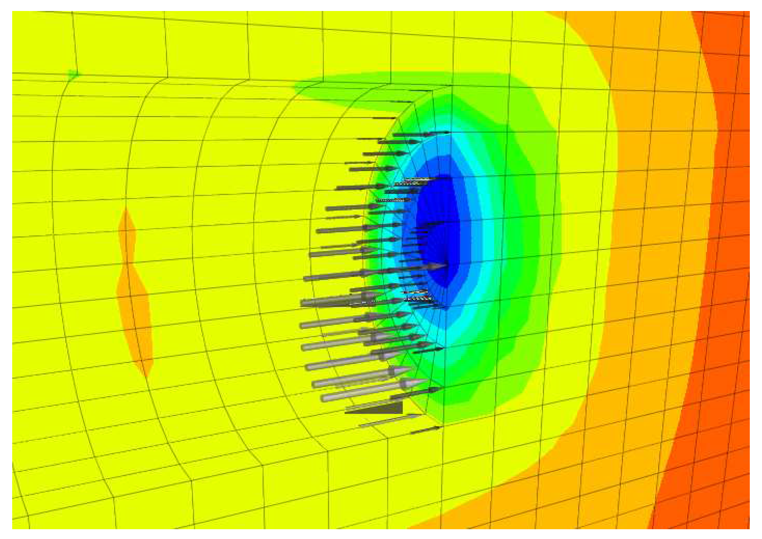
Table 5. The displacements are fixed in the horizontal direction at the vertical boundaries and in the vertical direction at the bottom. The excavation is performed by removing the elements corresponding to the excavated soil. The support provided by the tunnel lining is simulated by fixing the displacement at the excavation boundaries. The support pressure is provided by applying a linearly increasing external pressure onto the tunnel face (
Figure 11). This pressure is equal to 50, 100, 150, 200 or 250 kPa at the tunnel axis and increases linearly with depth according to the unit weight of the support medium
kN/m³. The support medium consists of excavated soil and additives for EPB machines or slurry suspension for SPB and mixshield machines [
118]. The surface settlement is measured at the gridpoints situated on the surface every 10 m.
In the analytical environment, the surface settlement is calculated at every excavation round. In reality, the cumulative surface settlement depends on the previous excavation steps. Hence, the settlement increase is considered in the finite difference environment to account for the effect of the tunnel face support pressure at each step. The settlement reward for state t is thus expressed as the maximum settlement difference between the excavation steps of all the j-th measuring point along the soil surface.
Finally, the game over condition is not triggered by excessively large settlements, such as in the analytical environment, but by the divergence of the numerical solution.
Within the framework of transfer learning, the application of a machine learning model to a similar but unrelated problem [
119], it is worth studying if and to what extent the algorithm used for the analytical environment can be deployed on the finite difference environment. The cumulative reward of
is obtained in this environment if the support pressure is predicted with the algorithm trained in the analytical environment. This result is compared by retraining the model with
in the finite difference environment. As it takes approximately 30 minutes to complete one episode, this training is computationally costly. Therefore, the model is trained only for 50 episodes or about 90% of the expected peak cumulative reward according to
Figure 9.
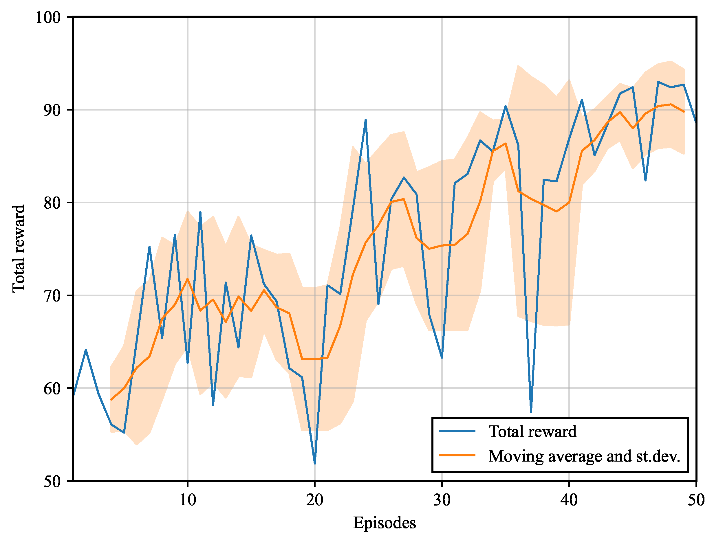
The cumulative reward obtained at each episode is shown in
Figure 12. For the first 20 episodes, the cumulative reward oscillates across approximately 65, corresponding to the reward obtained by using the model trained in the analytical environment. The cumulative reward oscillates across 75 between episodes 20 and 37 and stabilises at about 90 from episode 40.
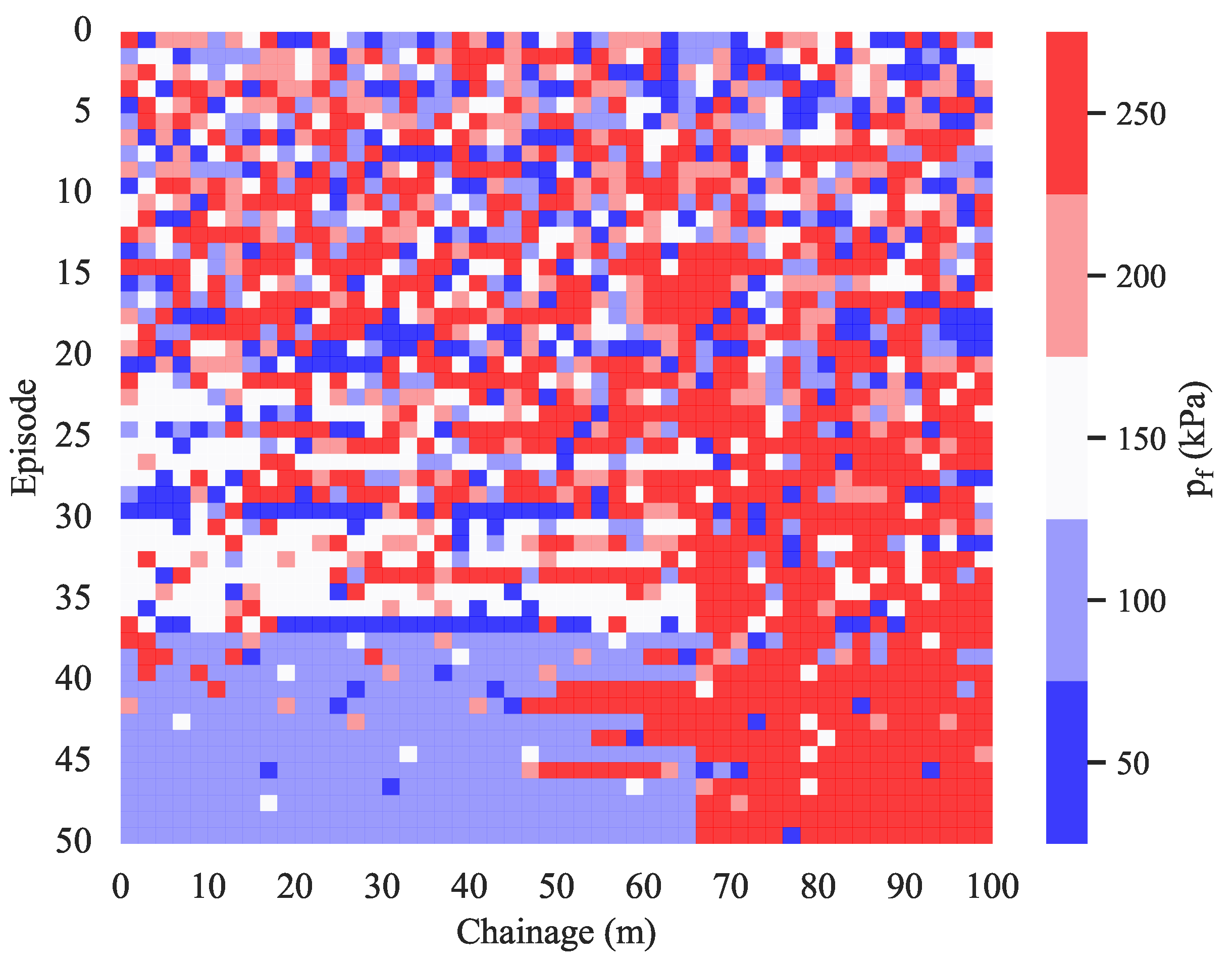
Figure 13 shows the support pressures chosen along the chainage at each episode. This visualisation shows how the initial randomness begins to vanish at episode 20 where the first patterns start to emerge. In particular, the agent learns that the optimal support pressure between chainage 65 and 100 m is 250 kPa. It is also interesting to notice, that, between episodes 20 and 37, the agent preferably chooses a support pressure of 150 kPa between chainage 0 and 65 m. Starting from episode 37, it is evident that the optimal support pressure for the first 65 m is 100 kPa. This is consistent with
Figure 12, where the cumulative reward starts increasing after episode 20 and increases again after episode 37.
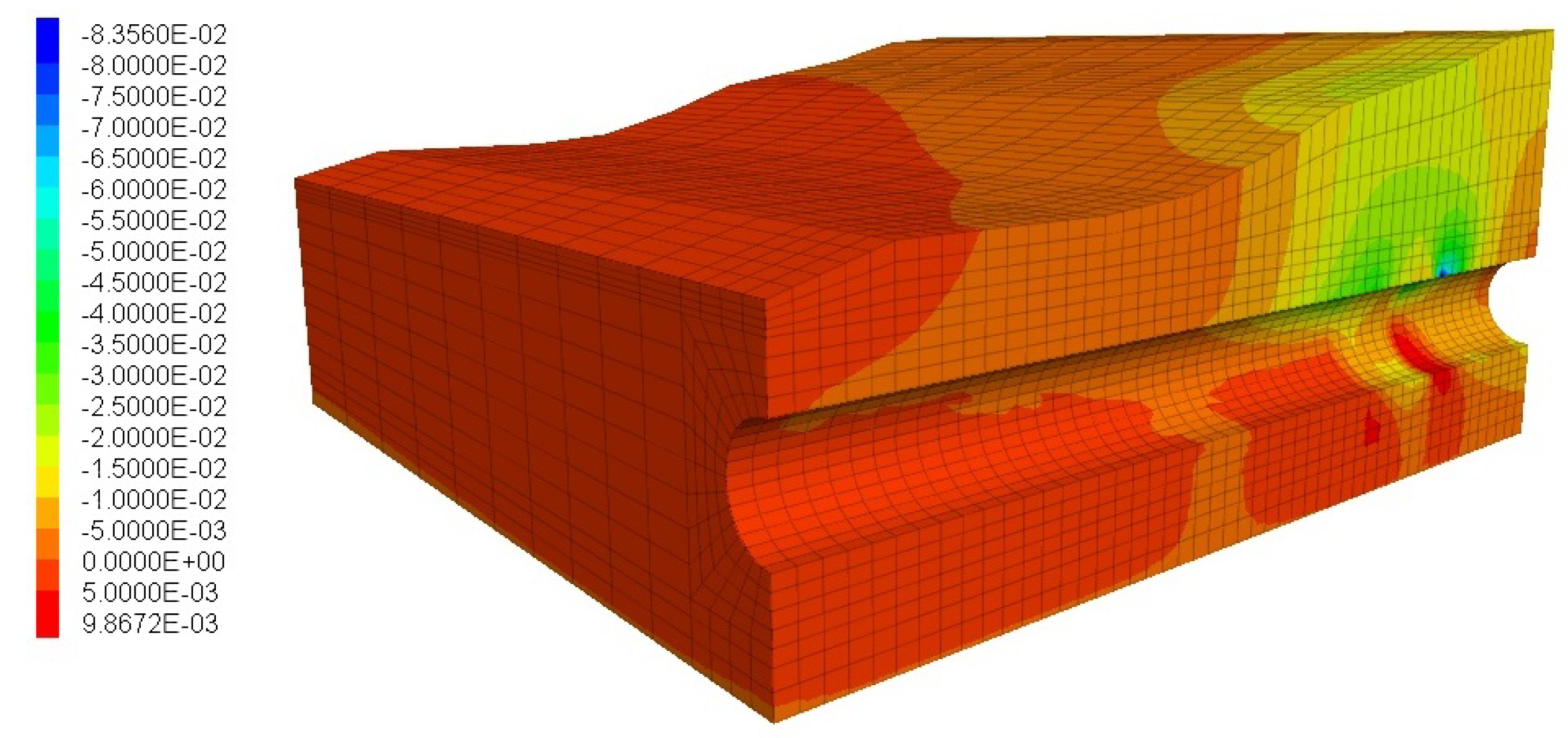
Figure 14 shows the settlement after the last episode is completed. The surface settlement is up to 1 cm in the first 65 m of excavation and up to 2 cm in the last 35 m. Hence, it is evident that the actions chosen by the agent keep the settlement within reasonable limits.
From the previous analysis, it seems that the model developed in the analytical environment can be transferred to the finite difference environment provided that the model is retrained. These results are discussed in the next section.
4. Discussion
The results show that our model can optimise the support pressure by simultaneously control surface settlement within a reasonable threshold in both analytical and finite difference environments. Implementing model training in an analytical environment is relatively simple and a large number of episodes can be completed fairly fast. Moreover, this class of environments allows for hyperparameter tuning. On the other hand, reinforcement learning training in the finite difference environment (or, more generically, in numerical environments) is rather costly, see also [
36]. Therefore, transfer learning is employed for hyperparameter tuning. As shown in the previous section, the model architecture and hyperparameters can be generally transferred to the finite difference environment, on the condition that retraining is performed starting from
.
Some limitations of this study can be highlighted and a strategy to amend them is outlined in the following. Firstly, albeit its use in engineering design, the finite difference environment cannot completely match reality. This is especially true in light of the simplifications considered in this study, such as the linear-elastic material law with Mohr-Coulomb failure criterion, the simulation of the tunnel lining as a zero displacement boundary condition, the absence of the ring gap and mortar and the deterministic soil properties values. These limitations can be overcome as follows:
The adoption of more advanced constitutive models, the simulation of the lining with shell elements and the simulation of the ring gap and mortar [
120,
121]. It is perhaps worth noting that different types of segments (in terms of concrete class and reinforcement) and ring gap mortar pressures are chosen in practice. Hence, two additional agents could be implemented to predict the segment types and mortar pressures.
The consideration of the spatial variability of soil properties with random fields, by varying the soil properties according to certain statistical distributions and correlation lengths [
122]. Since random fields further complicate the environment, more advanced reinforcement learning algorithms might be adopted, such as the C51 [
123]. Also, the definition of the state variables can be improved, e.g. by considering the soil properties in more than one point at each epoch.
The results match the expectation that the agent can be trained to predict the tunnel face support pressure. However, it is striking that the agent does not appear to need any additional training when deployed on random geologies (
Section 3.2). This feature could be also theoretically tested with the finite difference environment. However, hyperparameter tuning with this environment is still computationally costly.
The results show that the DQN algorithm can be successfully used to control the tunnel support pressure and adapt to changes in the soil properties, such as variations in unit weight, cohesion, friction angle and Young’s modulus. One added value of the DQN in this context is that it can be used to develop more efficient and effective control strategies for maintaining tunnel face stability compared to traditional methods. The DQN has the capability to generalise to new situations, which can be useful in the case of changes in soil properties or overburden height. Furthermore, the DQN algorithm allows for an efficient use of the available data as it is not heavily dependent on its quality, which is a common problem with traditional methods.
5. Conclusions
In this study, the Deep Q-Network reinforcement learning algorithm is applied to control the tunnel face support pressure during excavation. The algorithm is tested against analytical as well as numerical environments. The analytical environment is used for hyperparameter tuning. The optimised model is used in the numerical environment.
It is found that:
The algorithm is capable of predicting the tunnel face support pressure that ensures stability and minimise settlements among a prescribed range of pressures. The algorithm can adapt to geological (soil properties) or geometrical (overburden) changes.
An analytical environment is used to optimise the algorithm. The optimal hyperparameters are found as (discount factor), (learning rate), (synchronisation frequency), (memory size) and (batch size). These hyperparameter values are effective also in the numerical environment.
Although the algorithm is trained in a static environment with constant geology, it is also effective with random geological settings. In particular, it is found that using the algorithm trained with a constant geology can be used for random geologies without retraining.
The maximum cumulative reward plateaus after 400 training episodes and about 90% of the peak performance is reached after 50 episodes.
The algorithm proves effective both in the analytical and in the more realistic numerical environment. Training is more computationally costly in the numerical environment. However, the hyperparameter values optimised in the analytical environment can be efficiently adopted.
Future research can consider more refined environments (in terms of constitutive models, simulation of the lining, ring gap and mortar and random fields), provide more advanced state definitions (by considering the soil property values of various points) and use more refined reinforcement learning algorithms.
In spite of some limitations of this method, this study shows that the tunnel face support pressure can be estimated by an intelligent agent for design and possibly even during building operations.
Author Contributions
Conceptualization, E.S.; methodology, E.S.; software, E.S.; validation, E.S. and C.G.; formal analysis, E.S. and C.G.; investigation, E.S.; resources, W.W.; data curation, E.S. and C.G.; writing—original draft preparation, E.S.; writing—review and editing, C.G. and W.W.; visualization, E.S.; supervision, W.W.; project administration, W.W.; funding acquisition, W.W. All authors have read and agreed to the published version of the manuscript.
Funding
This research was funded by the Otto Pregl Foundation for geotechnical fundamental research.
Data Availability Statement
Conflicts of Interest
The authors declare no conflict of interest.
Abbreviations
The following abbreviations are used in this manuscript:
| DQN |
Deep Q-Network |
| EPB |
Earth pressure balance shield |
| FDM |
Finite Difference Method |
| SPB |
Slurry pressure balance shield |
| TBM |
Tunnel boring machine |
References
- Anagnostou, G.; Kovári, K. The face stability of slurry-shield-driven tunnels. Tunnelling and Underground Space Technology 1994, 9, 165–174. [Google Scholar] [CrossRef]
- Anagnostou, G.; Kovári, K. Face stability conditions with earth-pressure-balanced shields. Tunnelling and Underground Space Technology 1996, 11, 165–173. [Google Scholar] [CrossRef]
- Chen, R.P.; Tang, L.J.; Yin, X.S.; Chen, Y.M.; Bian, X.C. An improved 3D wedge-prism model for the face stability analysis of the shield tunnel in cohesionless soils. Acta Geotechnica 2015, 10, 683–692. [Google Scholar] [CrossRef]
- DAUB. Recommendations for face support pressure calculations for shield tunnelling in soft ground. Guidelines, Deutscher Ausschuss für unterirdisches Bauen, Cologne, Germany, 2016.
- Davis, E.H.; Gunn, M.J.; Mair, R.J.; Seneviratine, H.N. The stability of shallow tunnels and underground openings in cohesive material. Géotechnique 1980, 30, 397–416. [Google Scholar] [CrossRef]
- Horn, N. Horizontal ground pressure on vertical faces of tunnel tubes. In Proceedings of the Landeskonferenz der Ungarischen Tiefbauindustrie; 1961. [Google Scholar]
- Leca, E.; Dormieux, L. Upper and lower bound solutions for the face stability of shallow circular tunnels in frictional material. Géotechnique 1990, 40, 581–606. [Google Scholar] [CrossRef]
- Mollon, G.; Dias, D.; Soubra, A.H. Rotational failure mechanisms for the face stability analysis of tunnels driven by a pressurized shield. International Journal for Numerical and Analytical Methods in Geomechanics, 35, 1363–1388. [CrossRef]
- Tang, X.W.; Liu, W.; Albers, B.; Savidis, S. Upper bound analysis of tunnel face stability in layered soils. Acta Geotechnica 2014, 9, 661–671. [Google Scholar] [CrossRef]
- Alagha, A.S.; Chapman, D.N. Numerical modelling of tunnel face stability in homogeneous and layered soft ground. Tunnelling and Underground Space Technology 2019, 94, 103096. [Google Scholar] [CrossRef]
- Augarde, C.E.; Lyamin, A.V.; Sloan, S.W. Stability of an undrained plane strain heading revisited. Computers and Geotechnics 2003, 30, 419–430. [Google Scholar] [CrossRef]
- Chen, R.; Tang, L.; Ling, D.; Chen, Y. Face stability analysis of shallow shield tunnels in dry sandy ground using the discrete element method. Computers and Geotechnics 2011, 38, 187–195. [Google Scholar] [CrossRef]
- Lü, X.; Zeng, S.; Zhao, Y.; Huang, M.; Ma, S.; Zhang, Z. Physical model tests and discrete element simulation of shield tunnel face stability in anisotropic granular media. Acta Geotechnica 2020, 15, 3017–3026. [Google Scholar] [CrossRef]
- Sterpi, D.; Cividini, A. A Physical and Numerical Investigation on the Stability of Shallow Tunnels in Strain Softening Media. Rock Mechanics and Rock Engineering 2004, 37, 277–298. [Google Scholar] [CrossRef]
- Ukritchon, B.; Keawsawasvong, S.; Yingchaloenkitkhajorn, K. Undrained face stability of tunnels in Bangkok subsoils. International Journal of Geotechnical Engineering 2017, 11, 262–277. [Google Scholar] [CrossRef]
- Vermeer, P.; Ruse, N.; Dolatimehr, A. Tunnel Heading Stability in Drained Ground. Felsbau 2002, 20. [Google Scholar]
- Zhang, Z.; Hu, X.; Scott, K.D. A discrete numerical approach for modeling face stability in slurry shield tunnelling in soft soils. Computers and Geotechnics 2011, 38, 94–104. [Google Scholar] [CrossRef]
- Ahmed, M.; Iskander, M. Evaluation of tunnel face stability by transparent soil models. Tunnelling and Underground Space Technology 2012, 27, 101–110. [Google Scholar] [CrossRef]
- peng Chen, R.; Li, J.; gang Kong, L.; jun Tang, L. Experimental study on face instability of shield tunnel in sand. Tunnelling and Underground Space Technology 2013, 33, 12–21. [Google Scholar] [CrossRef]
- Kirsch, A. Experimental investigation of the face stability of shallow tunnels in sand. Acta Geotechnica 2010, 5, 43–62. [Google Scholar] [CrossRef]
- Lü, X.; Zhou, Y.; Huang, M.; Zeng, S. Experimental study of the face stability of shield tunnel in sands under seepage condition. Tunnelling and Underground Space Technology 2018, 74, 195–205. [Google Scholar] [CrossRef]
- Chambon, P.; Corté, J. Shallow Tunnels in Cohesionless Soil: Stability of Tunnel Face. Journal of Geotechnical Engineering 1994, 120, 1148–1165. [Google Scholar] [CrossRef]
- Mair, R. Centrifugal modelling of tunnel construction in soft clay. PhD thesis, University of Cambridge, Cambridge, 1979.
- Soranzo, E.; Wu, W. Centrifuge Test of Face Stability of Shallow Tunnels in Unsaturated Soil. In Poromechanics V; American Society of Civil Engineers: Reston, Virginia, USA, 2013; pp. 1326–1335. [Google Scholar] [CrossRef]
- Achmet, Z.; Di Sarno, L. State-Of-The-Art Review Of Machine Learning Applications To Geotechnical Earthquake Engineering Problems. In Proceedings of the EASD Procedia EURODYN; 2020; pp. 3424–3437. [Google Scholar] [CrossRef]
- Jong, S.; Ong, D.; Oh, E. State-of-the-art review of geotechnical-driven artificial intelligence techniques in underground soil-structure interaction. Tunnelling and Underground Space Technology 2021, 113, 103946. [Google Scholar] [CrossRef]
- Ebid, A. 35 Years of (AI) in Geotechnical Engineering: State of the Art. Geotechnical and Geological Engineering 2021, 39, 637–690. [Google Scholar] [CrossRef]
- Moayedi, H.; Mosallanezhad, M.; Rashid, A.S.A.; Jusoh, W.A.W.; Muazu, M.A. A systematic review and meta-analysis of artificial neural network application in geotechnical engineering: theory and applications. Neural Computing and Applications 2020, 32, 495–518. [Google Scholar] [CrossRef]
- Shahin, M.A. State-of-the-art review of some artificial intelligence applications in pile foundations. Geoscience Frontiers 2016, 7, 33–44, Special Issue: Progress of Machine Learning in Geosciences. [Google Scholar] [CrossRef]
- Zhang, W.; Zhang, R.; Wu, C.; Goh, A.T.C.; Lacasse, S.; Liu, Z.; Liu, H. State-of-the-art review of soft computing applications in underground excavations. Geoscience Frontiers 2020, 11, 1095–1106. [Google Scholar] [CrossRef]
- Zhang, W.; Li, H.; Yongqin, L.; Liu, H.; Chen, Y.; Ding, X. Application of deep learning algorithms in geotechnical engineering: a short critical review. Artificial Intelligence Review 2021, 54, 1–41. [Google Scholar] [CrossRef]
- Marcher, T.; Erharter, G.; Winkler, M. Machine Learning in tunnelling – Capabilities and challenges. Geomechanics and Tunnelling 2020, 13, 191–198. [Google Scholar] [CrossRef]
- Shreyas, S.; Dey, A. Application of soft computing techniques in tunnelling and underground excavations: state of the art and future prospects. Innovative Infrastructure Solutions 2019, 4, 46. [Google Scholar] [CrossRef]
- Shahrour, I.; Zhang, W. Use of soft computing techniques for tunneling optimization of tunnel boring machines. Underground Space 2021, 6, 233–239. [Google Scholar] [CrossRef]
- Soranzo, E.; Guardiani, C.; Wu, W. A soft computing approach to tunnel face stability in a probabilistic framework. Acta Geotechnica 2022, 17, 1219–1238. [Google Scholar] [CrossRef]
- Soranzo, E.; Guardiani, C.; Wu, W. The application of reinforcement learning to NATM tunnel design. Underground Space, 2022; In Press. [Google Scholar] [CrossRef]
- Wang, X.; Lu, H.; Wei, X.; Wei, G.; Behbahani, S.; Iseley, T. Application of artificial neural network in tunnel engineering: a systematic review. IEEE Access 2020, 9125920, 119527–119543. [Google Scholar] [CrossRef]
- Zhang, W.Y.L.; Wu, C.; Li, H.; Goh, A.; Liu, H. Prediction of lining response for twin-tunnel construction in anisotropic clays using machine learning techniques. Underground Space 2022, 7, 122–133. [Google Scholar] [CrossRef]
- Afradi, A.; Ebrahimabadi, A.; Hallajian, T. Prediction of TBM Penetration Rate Using Fuzzy Logic, Particle Swarm Optimization and Harmony Search Algorithm. Geotechnical and Geological Engineering 2022, 40, 1513–1536. [Google Scholar] [CrossRef]
- Bai, X.D.; Cheng, W.C.; Li, G. A comparative study of different machine learning algorithms in predicting EPB shield behaviour: a case study at the Xi’an metro, China. Acta Geotechnica 2021, 16, 4061–4080. [Google Scholar] [CrossRef]
- Fu, X.; Zhang, L. Spatio-temporal feature fusion for real-time prediction of TBM operating parameters: A deep learning approach. Automation in Construction 2021, 132, 103937. [Google Scholar] [CrossRef]
- Kong, X.; Ling, X.; Tang, L.; Tang, W.; Zhang, Y. Random forest-based predictors for driving forces of earth pressure balance (EPB) shield tunnel boring machine (TBM). Tunnelling and Underground Space Technology 2022, 122, 104373. [Google Scholar] [CrossRef]
- Ren, J.; Wang, Z.; Pang, Y.; Yuan, Y. Genetic algorithm-assisted an improved AdaBoost double-layer for oil temperature prediction of TBM. Advanced Engineering Informatics 2022, 52, 101563. [Google Scholar] [CrossRef]
- Xiao, H.H.; Yang, W.K.; Hu, J.; Zhang, Y.P.; Jing, L.J.; Chen, Z.Y. Significance and methodology: Preprocessing the big data for machine learning on TBM performance. Underground Space 2022, 7, 680–701. [Google Scholar] [CrossRef]
- Yang, J.; Yagiz, S.; Liu, Y.J.; Laouafa, F. Comprehensive evaluation of machine learning algorithms applied to TBM performance prediction. Underground Space 2022, 7, 37–49. [Google Scholar] [CrossRef]
- Zhang, Q.; Yang, B.; Zhu, Y.; Guo, C.; Jiao, C.; Cai, A. Prediction Method of TBM Tunneling Parameters Based on Bi-GRU-ATT Model. Advances in Civil Engineering 2022, 2022, 3743472. [Google Scholar] [CrossRef]
- Bardhan, A.; Kardani, N.; GuhaRay, A.; Burman, A.; Samui, P.; Zhang, Y. Hybrid ensemble soft computing approach for predicting penetration rate of tunnel boring machine in a rock environment. Journal of Rock Mechanics and Geotechnical Engineering 2021, 13, 1398–1412. [Google Scholar] [CrossRef]
- Benardos, A.; Kaliampakos, D. Modelling TBM performance with artificial neural networks. Tunnelling and Underground Space Technology 2004, 19, 597–605. [Google Scholar] [CrossRef]
- Fattahi, H.; Babanouri, N. Applying Optimized Support Vector Regression Models for Prediction of Tunnel Boring Machine Performance. Geotechnical and Geological Engineering 2017, 35, 2205–2217. [Google Scholar] [CrossRef]
- Feng, S.; Chen, Z.; Luo, H.; Wang, S.; Zhao, Y.; Liu, L.; Ling, D.; Jing, L. Tunnel boring machines (TBM) performance prediction: A case study using big data and deep learning. Tunnelling and Underground Space Technology 2021, 110, 103636. [Google Scholar] [CrossRef]
- Fu, X.; Feng, L.; Zhang, L. Data-driven estimation of TBM performance in soft soils using density-based spatial clustering and random forest. Applied Soft Computing 2022, 120, 108686. [Google Scholar] [CrossRef]
- Mahmoodzadeh, A.; Nejati, H.R.; Mohammadi, M.; Hashim Ibrahim, H.; Rashidi, S.; Ahmed Rashid, T. Forecasting tunnel boring machine penetration rate using LSTM deep neural network optimized by grey wolf optimization algorithm. Expert Systems with Applications 2022, 209, 118303. [Google Scholar] [CrossRef]
- Gao, B.; Wang, R.; Lin, C.; Guo, X.; Liu, B.; Zhang, W. TBM penetration rate prediction based on the long short-term memory neural network. Underground Space 2021, 6, 718–731. [Google Scholar] [CrossRef]
- Li, J.; Li, P.; Guo, D.; Li, X.; Chen, Z. Advanced prediction of tunnel boring machine performance based on big data. Geoscience Frontiers 2021, 12, 331–338. [Google Scholar] [CrossRef]
- Mokhtari, S.; Mooney, M.A. Predicting EPBM advance rate performance using support vector regression modeling. Tunnelling and Underground Space Technology 2020, 104, 103520. [Google Scholar] [CrossRef]
- Wang, Y.; Wang, J.; Wang, R.; Liu, B.; Li, Y. TBM penetration rate prediction ensemble model based on full-scale linear cutting test. Tunnelling and Underground Space Technology 2023, 131, 104794. [Google Scholar] [CrossRef]
- Wang, Y.; Gao, X.; Jiang, P.; Guo, X.; Wang, R.; Guan, Z.; Chen, L.; Xu, C. An extreme gradient boosting technique to estimate TBM penetration rate and prediction platform. Bulletin of Engineering Geology and the Environment 2022, 81, 58. [Google Scholar] [CrossRef]
- Wei, M.; Wang, Z.; Wang, X.; Peng, J.; Song, Y. Prediction of TBM penetration rate based on Monte Carlo-BP neural network. Neural Computing and Applications 2021, 33, 603–611. [Google Scholar] [CrossRef]
- Xu, H.; Zhou, J.G.; Asteris, P.; Jahed Armaghani, D.; Tahir, M.M. Supervised Machine Learning Techniques to the Prediction of Tunnel Boring Machine Penetration Rate. Applied Sciences 2019, 9. [Google Scholar] [CrossRef]
- Zeng, J.; Roy, B.; Kumar, D.; Mohammed, A.S.; Armaghani, D.J.; Zhou, J.; Mohamad, E.T. Proposing several hybrid PSO-extreme learning machine techniques to predict TBM performance. Engineering with Computers 2021. [Google Scholar] [CrossRef]
- Zhang, Q.; Hu, W.; Liu, Z.; Tan, J. TBM performance prediction with Bayesian optimization and automated machine learning. Tunnelling and Underground Space Technology 2020, 103, 103493. [Google Scholar] [CrossRef]
- Zhang, Y.; Chen, J.; Han, S.; Li, B. Big Data-Based Performance Analysis of Tunnel Boring Machine Tunneling Using Deep Learning. Buildings 2022, 12. [Google Scholar] [CrossRef]
- Zhao, J.; Shi, M.; Hu, G.; Song, X.; Zhang, C.; Tao, D.; Wu, W. A Data-Driven Framework for Tunnel Geological-Type Prediction Based on TBM Operating Data. IEEE Access 2019, 7, 66703–66713. [Google Scholar] [CrossRef]
- Qin, S.; Xu, T.; Zhou, W.H. Predicting Pore-Water Pressure in Front of a TBM Using a Deep Learning Approach. International Journal of Geomechanics 2021, 21, 04021140. [Google Scholar] [CrossRef]
- Kim, D.; Pham, K.; Oh, J.Y.; Lee, S.J.; Choi, H. Classification of surface settlement levels induced by TBM driving in urban areas using random forest with data-driven feature selection. Automation in Construction 2022, 135, 104109. [Google Scholar] [CrossRef]
- Kim, D.; Kwon, K.; Pham, K.; Oh, J.Y.; Choi, H. Surface settlement prediction for urban tunneling using machine learning algorithms with Bayesian optimization. Automation in Construction 2022, 140, 104331. [Google Scholar] [CrossRef]
- Lee, H.K.; Song, M.K.; Lee, S.S. Prediction of Subsidence during TBM Operation in Mixed-Face Ground Conditions from Realtime Monitoring Data. Applied Sciences 2021, 11. [Google Scholar] [CrossRef]
- Erharter, G.H.; Hansen, T.F. Towards optimized TBM cutter changing policies with reinforcement learning. Geomechanics and Tunnelling 2022, 15, 665–670. [Google Scholar] [CrossRef]
- Liu, Y.; Huang, S.; Wang, D.; Zhu, G.; Zhang, D. Prediction Model of Tunnel Boring Machine Disc Cutter Replacement Using Kernel Support Vector Machine. Applied Sciences 2022, 12. [Google Scholar] [CrossRef]
- Mahmoodzadeh, A.; Mohammadi, M.; Hashim Ibrahim, H.; Nariman Abdulhamid, S.; Farid Hama Ali, H.; Mohammed Hasan, A.; Khishe, M.; Mahmud, H. Machine learning forecasting models of disc cutters life of tunnel boring machine. Automation in Construction 2021, 128, 103779. [Google Scholar] [CrossRef]
- Hou, S.; Liu, Y.; Zhuang, W.; Zhang, K.; Zhang, R.; Yang, Q. Prediction of shield jamming risk for double-shield TBM tunnels based on numerical samples and random forest classifier. Acta Geotechnica 2022. [Google Scholar] [CrossRef]
- Lin, P.; Xiong, Y.; Xu, Z.; Wang, W.; Shao, R. Risk assessment of TBM jamming based on Bayesian networks. Bulletin of Engineering Geology and the Environment 2021, 81, 47. [Google Scholar] [CrossRef]
- Liu, M.; Liao, S.; Yang, Y.; Men, Y.; He, J.; Huang, Y. Tunnel boring machine vibration-based deep learning for the ground identification of working faces. Journal of Rock Mechanics and Geotechnical Engineering 2021, 13, 1340–1357. [Google Scholar] [CrossRef]
- Wellmann, F.; Amann, F.; de la Varga, M.; Chudalla, N. Automated geological model updates during TBM operation – An approach based on probabilistic machine learning concepts. Geomechanics and Tunnelling 2022, 15, 635–641. [Google Scholar] [CrossRef]
- Erharter, G.H.; Marcher, T. On the pointlessness of machine learning based time delayed prediction of TBM operational data. Automation in Construction 2021, 121, 103443. [Google Scholar] [CrossRef]
- Sheil, B. Discussion of “on the pointlessness of machine learning based time delayed prediction of TBM operational data” by Georg H. Erharter and Thomas Marcher. Automation in Construction 2021, 124, 103559. [Google Scholar] [CrossRef]
- International Business Machines. Supervised Learning, 2020. https://www.ibm.com/cloud/learn/supervised-learning.
- Mnih, V.; Kavukcuoglu, K.; Silver, D.; Rusu, A.A.; Veness, J.; Bellemare, M.G.; Graves, A.; Riedmiller, M.; Fidjeland, A.K.; Ostrovski, G.; et al. Human-level control through deep reinforcement learning. Nature 2015, 518, 529–533. [Google Scholar] [CrossRef]
- Schrittwieser, J.; Antonoglou, I.; Hubert, T.; Simonyan, K.; Sifre, L.; Schmitt, S.; Guez, A.; Lockhart, E.; Hassabis, D. Graepel, T.; Lillicrap, T.; et al. Mastering Atari, Go, chess and shogi by planning with a learned model. Nature 2020, 588, 604–612. [Google Scholar] [CrossRef] [PubMed]
- Silver, D.; Huang, A.; Maddison, C.; Guez, A.; Sifre, L.; van den Driessche, G.; Schrittwieser, J.; Antonoglou, I.; Panneershelvam, V.; Lanctot, M.; et al. Mastering the game of Go with deep neural networks and tree search. Nature 2016, 529, 484–503. [Google Scholar] [CrossRef] [PubMed]
- Silver, D.; Schrittwieser, J.; Simonyan, K.; Antonoglou, I.; Huang, A.; Guez, A.; Hubert, T.; Baker, L.L.M.; Bolton, A.; et al. Mastering the game of Go without human knowledge. Nature 2017, 550, 354–370. [Google Scholar] [CrossRef] [PubMed]
- Silver, D.; Hubert, T.; Schrittwieser, J.; Antonoglou, I.; Lai, M.; Guez, A.; Lanctot, M.; Sifre, L.; Kumaran, D.; Graepel, T.; et al. A general reinforcement learning algorithm that masters chess, shogi, and Go through self-play. Science 2018, 362, 1140–1144. [Google Scholar] [CrossRef] [PubMed]
- Shahrabi, J.; Adibi, M.; Mahootchi, M. Computers and Industrial Engineering. Nature 2017, 110, 75–82. [Google Scholar] [CrossRef]
- Ipek, E.; Mutlu, O.; Martínez, J.F.; Caruana, R. Self-Optimizing Memory Controllers: A Reinforcement Learning Approach. In Proceedings of the 2008 International Symposium on Computer Architecture; 2008; pp. 39–50. [Google Scholar] [CrossRef]
- Martinez, J.F.; Ipek, E. Dynamic Multicore Resource Management: A Machine Learning Approach. IEEE Micro 2009, 29, 8–17. [Google Scholar] [CrossRef]
- Li, L.; Chu, W.; Langford, J.; Schapire, R.E. A Contextual-Bandit Approach to Personalized News Article Recommendation. CoRR, 2010; abs/1003.0146. [Google Scholar]
- Theocharous, G.; Thomas, P.S.; Ghavamzadeh, M. Personalized Ad Recommendation Systems for Life-Time Value Optimization with Guarantees. Proceedings of the Proceedings of the 24th International Conference on Artificial Intelligence, AAAI Press, 2015, IJCAI’15. 1806–1812.
- Kiran, B.R.; Sobh, I.; Talpaert, V.; Mannion, P.; Sallab, A.A.A.; Yogamani, S.K.; Pérez, P. Deep Reinforcement Learning for Autonomous Driving: A Survey. CoRR, 2002; abs/2002.00444. [Google Scholar]
- Gao, X. Deep reinforcement learning for time series: playing idealized trading games. CoRR, 2018; abs/1803.03916. [Google Scholar]
- Paulus, R.; Xiong, C.; Socher, R. A Deep Reinforced Model for Abstractive Summarization. CoRR, 2017; abs/1705.04304. [Google Scholar]
- Yu, C.; Liu, J.; Nemati, S. Reinforcement Learning in Healthcare: A Survey. CoRR, 2019; abs/1908.08796. [Google Scholar]
- Mousavi, S.; Schukat, M.; Howley, E. Deep Reinforcement Learning: An Overview. In Proceedings of the Proceedings of SAI Intelligent Systems Conference (IntelliSys) 2016, 2018, pp. 426–440. [Google Scholar] [CrossRef]
- Erharter, G.; Marcher, T.; Hansen, T.; Liu, Z. Reinforcement learning based process optimization and strategy development in conventional tunnelling. Automation in Construction 2021, 127, 103701. [Google Scholar] [CrossRef]
- Zhang, P.; Li, H.; Ha, Q.; Yin, Z.Y.; Chen, R.P. Reinforcement learning based optimizer for improvement of predicting tunneling-induced ground responses. Advanced Engineering Informatics 2020, 45, 101097. [Google Scholar] [CrossRef]
- Van Rossum, G.; Drake, F.L. Python 3 Reference Manual; CreateSpace: Scotts Valley, CA, 2009. [Google Scholar]
- Andrew, A. Reinforcement Learning: An Introduction. Kybernetes 1998, 27, 1093–1096. [Google Scholar] [CrossRef]
- Bowyer, C. Characteristics of Rewards in Reinforcement Learning, 2022. https://medium.com/mlearning-ai/characteristics-of-rewards-in-reinforcement-learning-f5722079aef5.
- Singh, N. A Comprehensive Guide to Reinforcement Learning. https://www.analyticsvidhya.com/blog/2021/10/a-comprehensive-guide-to-reinforcement-learning, 2021. Accessed: 2022-05-18.
- Gütter, W.; Jäger, M.; Rudigier, G.; Weber, W. TBM versus NATM from the contractor’s point of view. Geomechanics and Tunnelling 2011, 4, 327–336. [Google Scholar] [CrossRef]
- Schuck, N.W.; Wilson, R.; Niv, Y. Chapter 12 - A State Representation for Reinforcement Learning and Decision-Making in the Orbitofrontal Cortex. In Goal-Directed Decision Making; Morris, R.; Bornstein, A.; Shenhav, A., Eds.; Academic Press, 2018; pp. 259–278. [CrossRef]
- Kit Machine. Is Domain Knowledge Important for Machine Learning?, 2022. https://www.kit-machines.com/domain-knowledge-machine-learning/.
- Leca, E.; New, B. Settlements induced by tunneling in Soft Ground. Tunnelling and Underground Space Technology 2007, 22, 119–149. [Google Scholar] [CrossRef]
- ITAtech Activity Group Investigation. Geophysical Ahead Investigation Methods Seismic Methods. Technical Report ITAtech Report No. 10, International Tunnelling Association, Salt Lake City, UT, 2018.
- Shirlaw, N. Setting operating pressures for TBM tunnelling. In Proceedings of the HKIE Geotechnical Division Annual Seminar, 2012: Geotechnical Aspects of Tunnelling for Infrastructure; The Hong Kong Institution of Engineers: Hong Kong, 2012; pp. 7–28. [Google Scholar]
- Virtanen, P.; Gommers, R.; Oliphant, T.E.; Haberland, M.; Reddy, T.; Cournapeau, D.; Burovski, E.; Peterson, P.; Weckesser, W.; Bright, J.; et al. SciPy 1.0: Fundamental Algorithms for Scientific Computing in Python. Nature Methods 2020, 17, 261–272. [Google Scholar] [CrossRef]
- Li, Y. Deep Reinforcement Learning: An Overview. CoRR, 2017; abs/1701.07274. [Google Scholar]
- Mnih, V.; Kavukcuoglu, K.; Silver, D.; Graves, A.; Antonoglou, I.; Wierstra, D.; Riedmiller, M. Playing Atari with Deep Reinforcement Learning. ArXiv 2013. [Google Scholar]
- Paszke, A.; Gross, S.; Massa, F.; Lerer, A.; Bradbury, J.; Chanan, G.; Killeen, T.; Lin, Z.; Gimelshein, N.; Antiga, L.; et al. , PyTorch: An Imperative Style, High-Performance Deep Learning Library. In Advances in Neural Information Processing Systems; Curran Associates, 2019; Vol. 32, pp. 8024–8035.
- Zai, A.; Brown, B. Deep Reinforcement Learning in Action; Manning: New York, U.S.A, 2020. [Google Scholar]
- Soranzo, E.; Guardiani, C.; Saif, A.; Wu, W. A Reinforcement Learning approach to the location of the non-circular critical slip surface of slopes. Computers & Geosciences 2022, 166, 105182. [Google Scholar] [CrossRef]
- Lin, L. Self-improving reactive agents based on reinforcement learning, planning and teaching. Machine Learning 1992, 8, 293–321. [Google Scholar] [CrossRef]
- McCloskey, M.; Cohen, N.J. Catastrophic Interference in Connectionist Networks: The Sequential Learning Problem. In Psychology of Learning and Motivation; Bower, G.H., Ed.; Academic Press, 1989; Vol. 24, pp. 109–165. [CrossRef]
- Alsahly, A.; Stascheit, J.; Meschke, G. Advanced finite element modeling of excavation and advancement processes in mechanized tunneling. Advances in Engineering Software 2016, 100, 198–214. [Google Scholar] [CrossRef]
- Demagh, R.; Emeriault, F. 3D Modelling of Tunnel Excavation Using Pressurized Tunnel Boring Machine in Overconsolidated Soils. Studia Geotechnica et Mechanica 2014, 35, 3–17. [Google Scholar] [CrossRef]
- Hasanpour, R. Advance numerical simulation of tunneling by using a double shield TBM. Computers and Geotechnics 2014, 57, 37–52. [Google Scholar] [CrossRef]
- Hasanpour, R.; Rostami, J.; Ünver, B. 3D finite difference model for simulation of double shield TBM tunneling in squeezing grounds. Tunnelling and Underground Space Technology 2014, 40, 109–126. [Google Scholar] [CrossRef]
- Itasca Consulting Group. FLAC3D (Fast Lagrangian Analysis of Continua); Itasca Consulting Group: Minneapolis, 2009. [Google Scholar]
- Dias, T.G.S.; Bezuijen, A. TBM Pressure Models – Observations, Theory and Practice. In Proceedings of the Volume 5: Geotechnical Synergy in Buenos Aires 2015; Sfriso, A.O. et al.., Ed. IOS Press, Advances in Soil Mechanics and Geotechnical Engineering; 2015; pp. 347–375. [Google Scholar] [CrossRef]
- Vilalta, R.; Giraud-Carrier, C.; Brazdil, P.; Soares, C. , MA, 2010; pp. 545–548. https://doi.org/https://doi.org/10.1007/978-0-387-30164-8_401.Transfer. In Encyclopedia of Machine Learning; Springer US: Boston, MA, 2010; pp. 545–548. [Google Scholar] [CrossRef]
- Kasper, T.; Meschke, G. A 3D finite element simulation model for TBM tunnelling in soft ground. International Journal for Numerical and Analytical Methods in Geomechanics, 28, 1441–1460. [CrossRef]
- Kasper, T.; Meschke, G. On the influence of face pressure, grouting pressure and TBM design in soft ground tunnelling. Tunnelling and Underground Space Technology 2006, 21, 160–171. [Google Scholar] [CrossRef]
- Fenton, G.; Griffiths, D. Risk Assessment in Geotechnical Engineering; John Wiley and Sonds: United States, 2008. [Google Scholar] [CrossRef]
- Bellemare, M.G.; Dabney, W.; Munos, R. A Distributional Perspective on Reinforcement Learning. CoRR, 2017; abs/1707.06887. [Google Scholar] [CrossRef]
- Anagnostou, G. The contribution of horizontal arching to tunnel face stability. Geotechnik 2012, 35, 34–44. [Google Scholar] [CrossRef]
- Flora, M.; Weiser, T.; Zech, P.; Fontana, A.; Ruepp, A.; Bergmeister, K. Added value in mechanized tunnelling by intelligent systems. Geomechanics and Tunnelling 2021, 14, 592–599. [Google Scholar] [CrossRef]
- Herrenknecht, AG. Mixshield, 2022. https://www.herrenknecht.com/en/products/productdetail/mixshield/.
- Huang, X.; Zhang, Q.; Liu, Q.; Liu, X.; Liu, B.; Wang, J.; Yin, X. A real-time prediction method for tunnel boring machine cutter-head torque using bidirectional long short-term memory networks optimized by multi-algorithm. Journal of Rock Mechanics and Geotechnical Engineering 2022, 14, 798–812. [Google Scholar] [CrossRef]
- International Business Machines. Machine Learning, 2020. https://www.ibm.com/cloud/learn/machine-learning.
- Kim, C.; Bae, G.; Hong, S.; Park, C.; Moon, H.; Shin, H. Neural network based prediction of ground surface settlements due to tunnelling. Computers and Geotechnics 2001, 28, 517–547. [Google Scholar] [CrossRef]
- Liu, X.; Shao, C.; Ma, H.; Liu, R. Optimal earth pressure balance control for shield tunneling based on LS-SVM and PSO. Automation in Construction 2011, 20, 321–327. [Google Scholar] [CrossRef]
- Mahmoodzadeh, A.; Nejati, H.R.; Mohammadi, M.; Ibrahim, H.H.; Rashidi, S.; Ibrahim, B.F. Forecasting Face Support Pressure During EPB Shield Tunneling in Soft Ground Formations Using Support Vector Regression and Meta-heuristic Optimization Algorithms. Rock Mechanics and Rock Engineering 2022, 55, 6367–6386. [Google Scholar] [CrossRef]
- Möller, S. Tunnel induced settlements and structural forces in linings. PhD thesis, University of Stuttgart, 2006.
- Shao, C.; Lan, D. Optimal control of an earth pressure balance shield with tunnel face stability. Automation in Construction 2014, 46, 22–29. [Google Scholar] [CrossRef]
- Xu, C.; Liu, X.; Wang, E.; Wang, S. Prediction of tunnel boring machine operating parameters using various machine learning algorithms. Tunnelling and Underground Space Technology 2021, 109, 103699. [Google Scholar] [CrossRef]
- Yeh, I.C. Application of neural networks to automatic soil pressure balance control for shield tunneling. Automation in Construction 1997, 5, 421–426. [Google Scholar] [CrossRef]
- Zhao, K.; Janutolo, M.; Barla, G. A Completely 3D Model for the Simulation of Mechanized Tunnel Excavation. Rock Mechanics and Rock Engineering 2012, 45, 475–497. [Google Scholar] [CrossRef]
- Zhou, C.; Ding, L.; He, R. PSO-based Elman neural network model for predictive control of air chamber pressure in slurry shield tunneling under Yangtze River. Automation in Construction 2013, 36, 208–217. [Google Scholar] [CrossRef]
Figure 1.
Random soil property values of the analytical environment with constant geology: (a) Unit soil weight. (b) Cohesion. (c) Friction angle. (d) Young’s modulus.
Figure 1.
Random soil property values of the analytical environment with constant geology: (a) Unit soil weight. (b) Cohesion. (c) Friction angle. (d) Young’s modulus.
Figure 2.
Tunnel face failure mechanism and forces acting on the sliding wedge according to [
4].
Figure 2.
Tunnel face failure mechanism and forces acting on the sliding wedge according to [
4].
Figure 3.
Architecture of the Deep Neural Network used for the choice of the support pressure based on the expected rewards and given the state of the TBM in the environment.
Figure 3.
Architecture of the Deep Neural Network used for the choice of the support pressure based on the expected rewards and given the state of the TBM in the environment.
Figure 4.
Rewards of the analytical environment with constant geology: (a) Cumulative reward vs. no. of episode; moving average and interval of range ±one standard deviation of ten episodes. (b) Cumulative reward vs. excavation step for all episodes.
Figure 4.
Rewards of the analytical environment with constant geology: (a) Cumulative reward vs. no. of episode; moving average and interval of range ±one standard deviation of ten episodes. (b) Cumulative reward vs. excavation step for all episodes.
Figure 5.
Required and provided support pressures and settlement in the analytical environment with constant geology at episode (a) 1, (b) 50 and (c) 100.
Figure 5.
Required and provided support pressures and settlement in the analytical environment with constant geology at episode (a) 1, (b) 50 and (c) 100.
Figure 6.
Cohesion values of the analytical environment with random geologies. (a) Episode 2. (b) Episode 3. (e) Episode 4. (d) Episode 5.
Figure 6.
Cohesion values of the analytical environment with random geologies. (a) Episode 2. (b) Episode 3. (e) Episode 4. (d) Episode 5.
Figure 7.
Rewards of the random environment: (a) Cumulative reward vs. no. of episode; moving average and interval of range ±one standard deviation of ten episodes. (b) Cumulative reward vs. excavation step for all episodes.
Figure 7.
Rewards of the random environment: (a) Cumulative reward vs. no. of episode; moving average and interval of range ±one standard deviation of ten episodes. (b) Cumulative reward vs. excavation step for all episodes.
Figure 8.
Required and provided support pressures and settlement in the analytical environment with random geologies at episode (a) 1, (b) 50 and (c) 100.
Figure 8.
Required and provided support pressures and settlement in the analytical environment with random geologies at episode (a) 1, (b) 50 and (c) 100.
Figure 9.
Effect of the number of episodes on the maximum cumulative reward.
Figure 9.
Effect of the number of episodes on the maximum cumulative reward.
Figure 10.
FLAC3D three-dimensional model. The colours represent the randomly generated soil layers 1 (yellow), 2 (green) and 3 (orange)
Figure 10.
FLAC3D three-dimensional model. The colours represent the randomly generated soil layers 1 (yellow), 2 (green) and 3 (orange)
Figure 11.
Detail of the horizontal displacement at the tunnel face and linearly increasing support pressure.
Figure 11.
Detail of the horizontal displacement at the tunnel face and linearly increasing support pressure.
Figure 12.
Rewards of the finite difference environment. Cumulative reward vs. no. of episode; moving average and interval of range ±one standard deviation for the last ten episodes.
Figure 12.
Rewards of the finite difference environment. Cumulative reward vs. no. of episode; moving average and interval of range ±one standard deviation for the last ten episodes.
Figure 13.
Support pressure chosen by the agent along the chainage for every episode.
Figure 13.
Support pressure chosen by the agent along the chainage for every episode.
Figure 14.
Computed vertical displacement at the last episode (in metres).
Figure 14.
Computed vertical displacement at the last episode (in metres).
Table 1.
Summary of the rewards associated with the outcomes of the actions.
Table 1.
Summary of the rewards associated with the outcomes of the actions.
| Outcome |
Reward |
| Excavation round |
|
| Choice of the tunnel face support pressure |
|
| Additional soil surface settlement |
|
Soil surface settlement > 10 cm or
divergence of the calculation |
and game over |
| Completed excavation |
and end of the episode |
Table 2.
Range of the intervals of soil properties and their coefficient of variation for every 2 m excavation step.
Table 2.
Range of the intervals of soil properties and their coefficient of variation for every 2 m excavation step.
| Soil parameter |
Symbol |
Unit |
Minimum value |
Maximum value |
% Variation/m |
| Unit weight |
|
(kN/m³) |
11 |
24 |
|
| Cohesion |
c |
(kPa) |
0 |
20 |
|
| Friction angle |
|
(°) |
20 |
40 |
|
| Young’s modulus |
E |
(MPa) |
10 |
100 |
|
Table 3.
Results of the analysis of sensitivity to the hyperparameters.
Table 3.
Results of the analysis of sensitivity to the hyperparameters.
| Hyperpameter |
Values |
Max. Reward |
| Discount factor
|
0.01 |
621.0 |
| |
0.15 |
657.2 |
| |
0.2 |
622.2 |
| Learning rate
|
|
637.1 |
| |
|
657.2 |
| |
|
536.3 |
| Synchronisation frequency f
|
5 |
657.2 |
| |
10 |
644.2 |
| |
15 |
652.1 |
| Memory size
|
5 |
647.3 |
| |
10 |
657.2 |
| |
15 |
562.8 |
| Batch size
|
5 |
630.0 |
| |
2 |
657.2 |
| |
1 |
609.3 |
Table 4.
Mean rewards and standard deviation of the random environment for different values of .
Table 4.
Mean rewards and standard deviation of the random environment for different values of .
|
Mean reward |
Standard deviation |
| 0.00 |
458.1 |
124.9 |
| 0.25 |
453.6 |
130.1 |
| 0.50 |
315.8 |
138.4 |
| 0.75 |
326.2 |
169.5 |
| 1.00 |
221.2 |
212.0 |
Table 5.
Soil property values assigned to the soil layers 1 (yellow), 2 (green) and 3 (orange) of
Figure 10.
Table 5.
Soil property values assigned to the soil layers 1 (yellow), 2 (green) and 3 (orange) of
Figure 10.
| Soil parameter |
Symbol |
Unit |
Layer 1 |
Layer 2 |
Layer 3 |
| Unit weight |
|
(kN/m³) |
23.0 |
13.7 |
15.9 |
| Cohesion |
c |
(kPa) |
14 |
1 |
11 |
| Friction angle |
|
(°) |
25 |
23 |
34 |
| Young’s modulus |
E |
(MPa) |
11 |
32 |
13 |
|
Disclaimer/Publisher’s Note: The statements, opinions and data contained in all publications are solely those of the individual author(s) and contributor(s) and not of MDPI and/or the editor(s). MDPI and/or the editor(s) disclaim responsibility for any injury to people or property resulting from any ideas, methods, instructions or products referred to in the content. |
© 2023 by the authors. Licensee MDPI, Basel, Switzerland. This article is an open access article distributed under the terms and conditions of the Creative Commons Attribution (CC BY) license (http://creativecommons.org/licenses/by/4.0/).
