Preprint
Article

Comparisons of Initial Condition Perturbation Methods for Regional Ensemble Forecasts of Wind Speed in Gansu of China

Altmetrics

Downloads

190

Views

64

Comments

0

Submitted:

13 February 2023

Posted:

14 February 2023

You are already at the latest version

Alerts
Abstract
This work compared the performance of three methods for constructing a regional ensemble prediction system (EPS) for wind speed forecasts: dynamical downscaling, breeding of growth modes (BGM), and blending method. The Weather Research and Forecasting (WRF) model was used to downscale the European Centre for Medium-range Weather Forecast (ECMWF) EPS. In addition, as the BGM method needs observation data for generating scaling factors, an alternative method for generating scaling factors was proposed to eliminate dependence on observation data. One-month tests between October 1st and October 30th, 2020, were implemented to evaluate the performance of three methods in the Gansu province of China. The results demonstrate that the blending method outperforms the other two methods. Furthermore, the difference in performance is evident mainly in early forecast lead time and becomes negligible as forecast time increases.
Keywords: 
Subject: Environmental and Earth Sciences  -   Atmospheric Science and Meteorology

1. Introduction

According to the Global Wind Energy Council (GWEC) [1], the total global capacity of wind power reached a milestone of 837 GW. Wind energy will likely continue to grow strongly and play a leading role in achieving a low-carbon or net-zero future. However, the large scale penetration of wind power also brings many challenges due to fluctuations and intermittency of wind power generation [2,3]. The wind forecast plays a critical role in overcoming these challenges [4,5,6]. One of the essential benefits of accurate wind forecast is to reduce grid stress and reserve requirements [7,8].
The wind forecast for energy generation and power system operations mainly focuses on the immediate short term of seconds to minutes, the short term of hours up to two days, and the medium term of 2 to 7 days as the power system operations are carried out within these time windows [9]. Nowadays, there are mainly three classes of wind forecasting methods. The first is the statistical method based on historical data, and the second is physics-based numerical weather prediction (NWP) models. The last one is the hybrid approach combining different approaches, such as combinations of statistical and physics-based approaches. The importance of different methods varies with the forecast lead time [10]. Hanifi et al. [11] systematically reviewed these approaches and concluded that NWP models significantly benefits for forecasts beyond 6 hours. However, NWP simulations are uncertain due to uncertainties in the initial conditions, limited understanding of the atmosphere's physical processes, and the atmospheric flow's chaotic nature [12,13]. The ensemble prediction system (EPS) is a promising way to estimate the forecast uncertainties [14,15].
The EPS is often made by perturbing initial conditions, and the perturbation methods applied by different global operational ensemble forecasting centers are different. At the National Centers for Environmental Prediction [NCEP, previously the National Meteorological Center (NMC)), Toth and Kalnay [16] introduced the breeding of growth modes (BGM) method based on the argument that fast-growing perturbations develop naturally in a data assimilation cycle [17]. The European Centre for Medium-range Weather Forecast (ECMWF) developed and implemented the Singular Vector (SV) method to identify the directions of the fastest growth [18,19]. The Canadian Meteorological Centre (CMC) developed an ensemble data assimilation method to produce different initial conditions for ensemble forecasts [20,21]. As a result of limited computing resources, the global EPS is usually run at coarser resolutions than deterministic forecasts. The NCEP global ensemble forecast system (GEFS) uses a 34 km horizontal resolution [22], while the CMC Global Ensemble Prediction System (GEPS) runs at a horizontal resolution of 39 km [23]. The ECMWF EPS uses the highest horizontal resolution at 18 km and 91 vertical levels, containing one control member and 50 perturbed members [24].
The region of interest for this study, Gansu province in China, is rich in wind resources [25] and has the world’s most giant onshore wind farms [26]. Unfortunately, Gansu is also the province with the most severe wind curtailment in China, discarding 10.4 TW h of potential wind power in 2016 [27]. According to Lew et al. [28], a 10% improve ment in wind forecasts could lead to a 4% reduction in curtailment and operation costs. Therefore, improving wind forecasts for wind farms in Gansu is very important. In addition, Gansu is located in northwest China and has a complex topography, requiring higher spatial resolutions to resolve topographic impact [8,29].
Given that the horizontal resolution of the global EPS is too coarse, it is necessary to build a regional EPS for an accurate wind forecast. The construction of the initial condition perturbations and lateral boundary condition (LBC) perturbations are crucial for a skillful regional EPS. The most common approach is the dynamical downscaling of a global EPS to the regional domain [30]. Because of its simplicity and low computational costs, this method is implemented by many NWP centers for regional operational EPS [31,32,33]. However, the dynamical downscaling method fails to represent the small-scale uncertainties resolved by the regional model [34]. Thus, researchers use regional versions of traditional perturbation methods such as BGM, SV, and ensemble transform Kalman filter (ETKF) [35,36] and that produce more information on small-scale uncertainties. Also, Caron [37] found that the mismatches between the initial condition perturbations and the LBC perturbations cause spurious perturbations. Therefore, a blending method was proposed to combine the regional model-based small-scale initial condition perturbations with large-scale perturbations from a global EPS [38,39]. Wang et al. [39] described the blending method implemented in the regional EPS, i.e. Aire Limitée Adaption dynamique Développement International-Limited Area Ensemble Forecasting (ALADIN-LAEF), and demonstrated that the blending method outperforms the dynamical downscaling and breeding method. Zhang et al. [40] also showed that the breeding method improved the ensemble spread and forecast skills of the Global/Regional Assimilation and Prediction Enhanced System (GRAPES) Regional EPS (GRAPES-REPS).
In this study, we use the Weather Research and Forecasting (WRF) model for dynamical downscaling of ECMWF EPS to generate large-scale perturbations and the BGM method to generate small-scale initial condition perturbations due to its clear meaning and low computational cost. As the BGM method requires using forecast error for calculating scaling factor and observations are not always available, we proposed an alternative to calculating the scaling factor. Additionally, we apply the blending method to combine perturbations of different scales and compare the wind forecast performance of dynamical downscaling, BGM, and blending in Gansu.
The paper is structured as follows: Section 2 describes the WRF model setup and regional EPS using dynamical downscaling, BGM, and blending methods. Section 3 introduces data and metrics for evaluation. Section 4 presents the evaluation results of day-ahead and ultra-short wind forecasts for one month. Finally, section 5 concludes the study with suggestions for future work from the results.

2. WRF Model Setup and Perturbation Methods Description

2.1. WRF Model Setup

The WRF model version 3.9.1 is used. As shown in Figure 1, the WRF model is configured with one single domain at a horizontal grid resolution of 8 km centered at 38° N in latitude and 101° E in longitude. The model used a terrain-following vertical coordinate with 55 vertical levels and a model top at 50 hPa. The ECMWF EPS is run four times per day, and only the ensemble forecast data initialized at 12 UTC is used to run the WRF model for 54 hours of forecasts. The physics parameterizations are selected following the same methodology presented in the [41]. The selected schemes include WRF Single-Moment 6-Class for microphysics [42], Bougeault-Lacarrère (BouLac) planetary boundary layer (PBL) scheme [43], Pleim-Xiu land surface model [44,45], Kain-Fritsch scheme for cumulus [46], and New Goddard for both longwave and shortwave radiation [47].

2.2. Description of the Initial Condition Perturbation Methods

As listed in Table 1, this study compared three initial condition perturbation methods: dynamical downscaling, BGM, and blending. The WRF model is used for dynamically downscaling all the 51 ensemble members of ECMWF EPS for initial condition and LBC perturbations.

2.2.1. BGM Method

The BGM method is an initial condition perturbation method widely applied for ensemble prediction. In this work , the classic BGM method is implemented following [48]. Firstly, an initial random perturbation determined by Equation (1) is added at a given time t :
P ( z ) = ω R E ( z )
where z is the state variable of the NWP model ( z could be T ,   U , or V representing the thermal and dynamic fields, respectively), and ω is an adjustment coefficient to control the magnitude of the initial random perturbations. R is a uniform random number in the interval [−1, 1]. E ( z ) is the root mean square error (RMSE) for variables at each layer.
Then, the model with both the unperturbed and perturbed initial condition is run for a short period (i.e., 12 hours for all the experiments in this paper). The difference between the control prediction with an unperturbed initial condition and the perturbation prediction with an unperturbed initial condition is calculated. As the difference increases with time, the difference is scaled down to have the same norm (e.g., amplitude) as the initial perturbation. This scaled difference is added to the analysis of the following time t + 1 . The process is repeated forward in time to generate the final perturbations until the growth rate of perturbations is saturated. The detailed calculations of perturbations are as follows:
p t + 1 = c t ( f t a f t s )
c t = E ( p t ) / E ( p t + 1 ' )
where p t + 1 is the perturbation at time t + 1 of the next cycle; f t + 1 a is the perturbed prediction, and f t + 1 s is the control prediction. c t is the scaling factor; E ( p t ) and E ( p t + 1 ' ) are RMSE at the beginning and end of the cycle period.
T Traditionally, observation data is needed to calculate the scaling factor. However, as observation data is not always available, we proposed to use the min-max scaling technique, a widely used normalization technique in machine learning, to scale the perturbations between a and a without observations:
p t + 1 = p t + 1 ' min ( p t + 1 ' ) max ( p t + 1 ' ) min ( p t + 1 ' ) 2 a a
where a = ω E ( z ) so that perturbations at the end of the cycle are of the same amplitude as initial perturbations.

2.2.1. Blending

The blending method combines the small-scale uncertainties resolved by WRF BGM and large-scale features from the global ensemble. Also, including perturbations from the global ensemble in the initial condition perturbation ensure that the initial condition is consistent with LBC provided by the global ensemble.
Here, the blending is implemented following the steps: (1) downscaling the global ensemble initial condition to the regional domain using the WRF model to get large-scale uncertainties; (2) sum the downscaled initial condition with perturbations generated by the WRF BGM described in Section 2.2.1.

3. Data and Metrics for Evaluation

3.1. Observation Data

The study period is from October 1st, 2020, to October 31st, 2020, for evaluation. We use hourly wind speed observations by anemometers installed at wind turbine hub height from 28 wind farms in Gansu, China. The WRF model output is interpolated to the turbine hub height to compare with the observation data. In addition, the wind speed forecast of the nearest grid point from the WRF domain is extracted to compare with wind turbine observations.

3.2. Evaluation Methods

According to the National Energy Bureau (NEB) regulation, day-ahead short-term and four-hours ahead wind forecasts are required [49]. Using the 12 UTC ECMWF data, the 28 to 51 hours forecast horizon represents the day-ahead forecast, while the 10 to 13 hours forecast horizon corresponds to the ultra-short term forecast.
To compare the performance of ensemble forecasts generated by the three initial condition perturbation methods, we applied several verification methods: RMSE and mean bias error (MBE) for the ensemble mean, ensemble spread [i.e., standard deviation (std)], continuous ranked probability score (CRPS) [50,51], and rank histograms [52]. These measures are calculated at the 1-hour frequency for wind speed forecasts following the equations below:
R M S E = 1 N ( W S p r e d W S o b s ) 2
M B E = 1 N ( W S p r e d W S o b s )
s t d = 1 N ( x p r e d x p r e d ¯ ) 2
where W S p r e d is the predicted wind speed ( W S ), W S o b s is the observed wind speed, and N is the number of pairs of forecast and observation. x p r e d is the ensemble member forecast, and x p r e d ¯ refers to the ensemble mean. RMSE and MBE of the ensemble mean describe the deterministic skill of the ensemble forecast. The ensemble spread is the std of the ensemble members with respect to the ensemble mean. When observations are unavailable, the ensemble spread can be used as a predictor of skills of the ensemble mean [53]. Small spread indicates low uncertainties, otherwise indicates high uncertainties.
The CRPS is defined as:
C R P S = [ F ( y ) F o ( y ) ] 2 d y
where F o ( y ) is an indicator function of which the value is 0 if the forecast variable y is less than the observation and one otherwise [54].
F o ( y ) = { 0 ,     y < o b s e r v e d   v a l u e 1 ,     y o b s e r v e d   v a l u e
The CRPS is a penalty score, and a smaller value of CRPS indicates a better ensemble forecast. The properscoring package in Python is used for calculating the CRPS in this work [55].
Additionally, the rank histogram is a valuable tool for examining ensemble reliability. It is generated by tallying the rank of verification (usually observation) relative to the forecast values of each ensemble member sorted in ascending order [52]. For a perfect EPS, the rank histogram should be flat. A U-shaped rank histogram generally indicates a lack of variability in the ensemble forecast, and an asymmetric shape (either J or L-shaped) indicates bias.

4. Results and Discussion

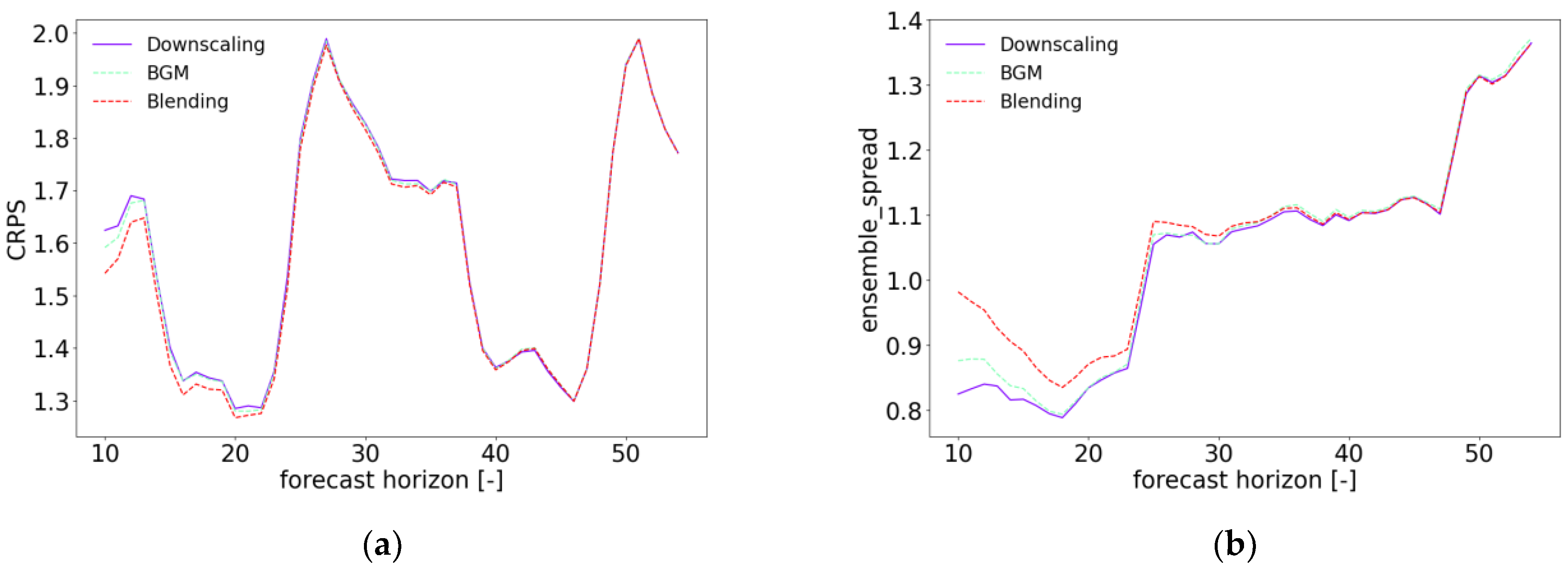
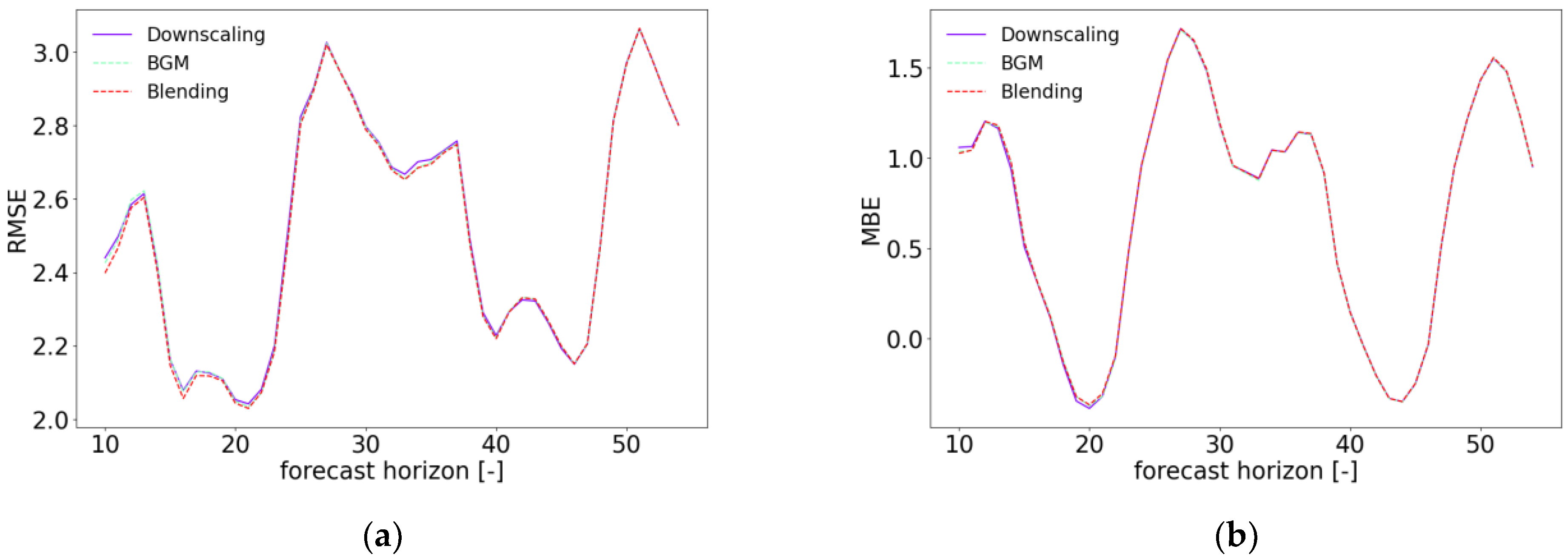
Figure 2 illustrates the one-month averaged CRPS and ensemble spread of wind speed forecast at turbine height for downscaling (solid purple lines), breeding (dashed green lines), and blending (dashed red lines) of ECMWF-EPS as a function of the forecast horizon from 10 to 54 hours. Overall, the blending ensemble shows the best performance with the smallest values of CRPS and the largest spread, especially within the forecast lead time between 10 and 25 hours. The BGM ensemble performs slightly better than the downscaling ensemble, with smaller values of RMSE and a larger spread, in the early forecast lead time. As all three ensembles use the same LBCS from ECMWF-EPS forecasts, it can be concluded that the BGM method is superior to the downscaling method, and the blending method takes advantage of both perturbation methods. After 25 hours, the difference in CRPS and ensemble spread among downscaling, BGM, and blending are almost negligible. These results suggest that the physics and boundary conditions dominate over initial condition perturbations in the long-term forecast in the study domain. As demonstrated in Figure 3, the RMSE and MBE of the ensemble mean of the downscaling, BGM, and blending ensemble for wind speed are very similar. However, during the earlier forecast lead time, the blending ensemble shows slightly smaller values than the downscaling and BGM ensemble.
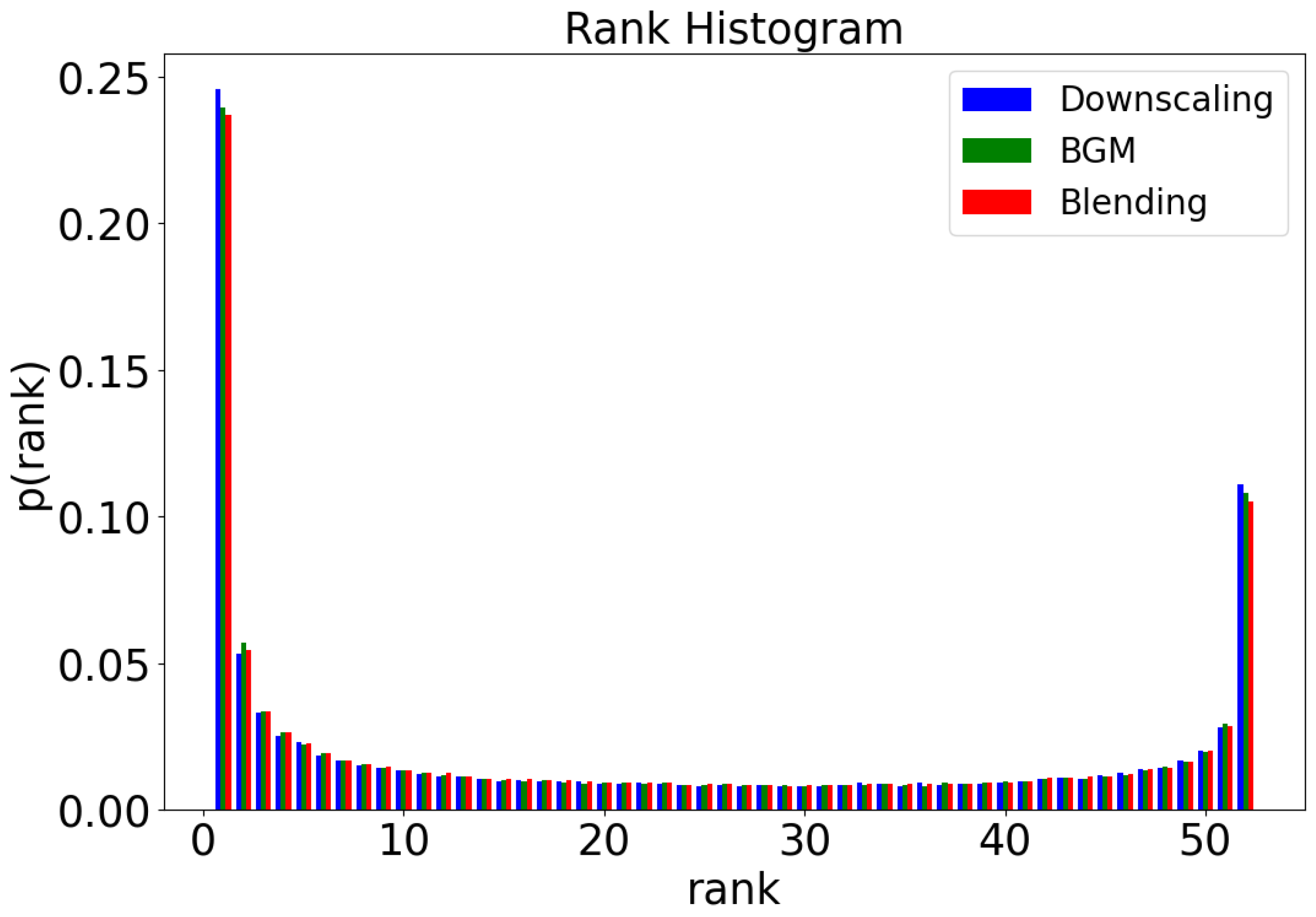
Figure 4 compares the rank histogram for the wind speed forecast of the forecast lead time from 10 to 54 hours among the downscaling (blue), BGM (green), and blending (red) ensemble. The U-shaped rank histogram of all three ensembles means that the three ensemble forecasts are under dispersive. However, the blending ensemble is flatter than the downscaling and BGM ensemble, indicating that the frequency that observations lay inside the ensemble is highest for the blending ensemble. The BGM ensemble is also comparatively flatter than the downscaling.
Table 2 summarizes the averaged RMSE and MBE of the ensemble mean of wind speed forecasts for the downscaling, BGM, and blending ensemble over the forecast horizons of 10 to 13 hours and 28 to 51 hours over one month. As seen from Table 2, the RMSE of the blending ensemble is smaller than the other two ensembles, with more difference over the earlier forecast lead time from 10 to 13 hours than the forecast lead time of 28 to 51 hours, consistent with Figure 3.
The analysis above demonstrates the overall improvement of the blending ensemble over the downscaling and BGM ensemble. Also, the effect of BGM and blending is evident mainly within an earlier forecast lead time of up to 25 hours. However, the effect could be extended to a longer forecast lead time if the domain of the study increases, as it will take longer for LBC to dominate over perturbations in initial conditions (this is beyond the scope of this study, thus not shown). Therefore, although the improvement in RMSE is not significant, it is still worth applying the blending method to improve the ensemble reliability of regional EPS [40].

5. Conclusions

In this study, we compared three methods to generate initial condition perturbations for building ensemble wind speed forecasts for the Gansu province of China, including dynamical downscaling, BGM and blending. The dynamical downscaling can produce large-scale perturbations by directly downscaling the ECMWF EPS using the WRF model. As we lack the observation data that the BGM method needs for generating the scaling factor periodically, we propose to use the min-max scaling method to scale the small-scale perturbations. The WRF BGM method can resolve small-scale perturbations, while the blending method can combine large-scale and small perturbations. Over the one-month testing period from October 1st to October 31st, 2020, the blending ensemble shows the best forecast skill, especially at the early forecast lead time. The CRPS, ensemble spread, and rank histogram of wind speed forecast demonstrate that the blending ensemble has a better probabilistic forecast. Furthermore, the difference among the three perturbation methods decreases as the forecast lead time becomes negligible after 25 hours. The RMSE and MBE comparisons of wind speed forecast also indicate that the blending ensemble is superior to downscaling and BGM ensemble.

Author Contributions

Conceptualization, X.Z.; methodology, X.Z.; software, X.Z.; validation, X.Z.; formal analysis, X.Z.; investigation, X.Z.; resources, X.Z.; data curation, X.Z.; writing—original draft preparation, X.Z.; writing—review and editing, X.Z.; visualization, X.Z.; supervision, Z.H., D.H., and Q.L.; project administration, Z.H., D.H., and Q.L.; funding acquisition, Z.H., D.H., and Q.L. All authors have read and agreed to the published version of the manuscript.

Funding

This research was funded by Envision Group Pte. Ltd.

Institutional Review Board Statement

Not applicable.

Informed Consent Statement

Not applicable.

Data Availability Statement

Where reasonable, the authors will provide data utilized in this study.

Acknowledgments

The authors acknowledge Envision Group Pte. Ltd. for funding the research, the European Centre for Medium-Range Weather Forecasts for the data used to drive the WRF model, and the Huawei cloud where the simulations were run.

Conflicts of Interest

The authors declare no conflict of interest.

References

  1. Global Wind Energy Council GWEC Global Wind Report 2022. 2021.
  2. Soman, S.S.; Zareipour, H.; Member, S.; Malik, O.; Fellow, L. A Review of Wind Power and Wind Speed Forecasting Methods With Different Time Horizons. In Proceedings of the North American Power Symposium, 2010. [Google Scholar] [CrossRef]
  3. Pinson, P. Wind Energy: Forecasting Challenges for Its Operational Management. Stat. Sci. 2013, 28, 564–585. [Google Scholar] [CrossRef]
  4. Jones, L.E. Strategies and Decision Support Systems for Integrating Variable Energy Resources in Control Centers for Reliable Grid Operations; 2011. [Google Scholar] [CrossRef]
  5. Dong, L.; Wang, L.; Farhan, S.; Gao, S.; Liao, X. Wind Power Day-Ahead Prediction with Cluster Analysis of NWP. Renew. Sustain. Energy Rev. 2016, 60, 1206–1212. [Google Scholar] [CrossRef]
  6. Chang, G.W.; Lu, H.J.; Chang, Y.R.; Lee, Y.D. An Improved Neural Network-Based Approach for Short-Term Wind Speed and Power Forecast. Renew. Energy 2017, 105, 301–311. [Google Scholar] [CrossRef]
  7. Potter, C.W.; Grimit, E.; Nijssen, B. Potential Benefits of a Dedicated Probabilistic Rapid Ramp Event Forecast Tool. 2009 IEEE/PES Power Syst. Conf. Expo. PSCE 2009 2009, 1–5. [Google Scholar] [CrossRef]
  8. Zhang, T.; Yan, P.; Li, Z.; Wang, Y.; Li, Y. Bias-Correction Method for Wind-Speed Forecasting. Meteorol. Zeitschrift 2019, 28, 293–304. [Google Scholar] [CrossRef]
  9. Foley, A.M.; Leahy, P.G.; Marvuglia, A.; McKeogh, E.J. Current Methods and Advances in Forecasting of Wind Power Generation. Renew. Energy 2012, 37, 1–8. [Google Scholar] [CrossRef]
  10. Santhosh, M.; Venkaiah, C.; Kumar, D.M.V. Current Advances and Approaches in Wind Speed and Wind Power Forecasting for Improved Renewable Energy Integration: A Review. Eng. Reports 2020, 1–20. [Google Scholar] [CrossRef]
  11. Hanifi, S.; Liu, X.; Lin, Z.; Lotfian, S. A Critical Review of Wind Power Forecasting Methods—Past, Present and Future. Energies 2020, 13, 1–24. [Google Scholar] [CrossRef]
  12. Edward, N. Lorenz Deterministic Nonperiodic Flow. J. Atmos. Sci. 1963, 20, 130–141. [Google Scholar]
  13. Zhang, H.; Pu, Z. Beating the Uncertainties: Ensemble Forecasting and Ensemble-Based Data Assimilation in Modern Numerical Weather Prediction. Adv. Meteorol. 2010, 2010, 1–10. [Google Scholar] [CrossRef]
  14. Gneiting, T.; Raftery, A.E. Atmospheric Science. Weather Forecasting with Ensemble Methods. Science (80-. ). 2005, 310, 248–249. [Google Scholar] [CrossRef]
  15. Bauer, P.; Thorpe, A.; Brunet, G. The Quiet Revolution of Numerical Weather Prediction. Nature 2015, 525, 47–55. [Google Scholar] [CrossRef]
  16. Toth, Z.; Kalnay, E. Ensemble Forecasting at NMC: The Generation of Perturbations. Bull. Am. Meteorol. Soc. 1993, 74, 2317–2330. [Google Scholar] [CrossRef]
  17. Buizza, R.; Houtekamer, P.L.; Toth, Z.; Pellerin, G.; Wei, M.; Zhu, Y. A Comparison of the ECMWF, MSC, and NCEP Global Ensemble Prediction Systems. Mon. Weather Rev. 2005, 133, 1076–1097. [Google Scholar] [CrossRef]
  18. Buizza, R.; Palmer, T.N. Palmer The Singular-Vector Sturcture of the Atmospheric Global Circulation. J. Atmos. Sci. 1995, 52, 1434–1456. [Google Scholar] [CrossRef]
  19. Molteni, F.; Buizza, R.; Palmer, T.N.; Petroliagis, T. The ECMWF Ensemble Prediction System: Methodology and Validation. Q. J. R. Meteorol. Soc. 1996, 122, 73–119. [Google Scholar] [CrossRef]
  20. Houtekamer, P.L.; Derome, J. Methods for Ensemble Prediction. Mon. Weather Rev. 1995, 123, 2181–2196. [Google Scholar] [CrossRef]
  21. Houtekamer, P.L.; Lefaivre, L.; Derome, J. A System Simulation Approach to Ensemble Prediction. Mon. Weather Rev. 1996, 124, 1225–1242. [Google Scholar] [CrossRef]
  22. Zhou, X.; Zhu, Y.; Hou, D.; Luo, Y.; Peng, J.; Wobus, R. Performance of the New NCEP Global Ensemble Forecast System in a Parallel Experiment. Weather Forecast. 2017, 32, 1989–2004. [Google Scholar] [CrossRef]
  23. Gagnon, S.; Deng, X. Ensemble Forecast Systems and Future Applications at MSC. In Proceedings of the 8th NCEP Ensemble User Workshop, 2019. [Google Scholar]
  24. Magnusson, L.; Bidlot, J.R.; Bonavita, M.; Brown, A.R.; Browne, P.A.; De Chiara, G.; Dahoui, M.; Lang, S.T.K.; McNally, T.; Mogensen, K.S.; et al. ECMWF Activities for Improved Hurricane Forecasts. Bull. Am. Meteorol. Soc. 2019, 100, 445–457. [Google Scholar] [CrossRef]
  25. Ye, Q.; Jiaqi, L.; Mengye, Z. Wind Curtailment in China and Lessons from the United States; 2018. [Google Scholar]
  26. NS Energy Staff Writer Profiling Ten of the Biggest Onshore Wind Farms in the World. Available online: https://www.nsenergybusiness.com/features/worlds-biggest-onshore-wind-farms/ (accessed on 23 March 2021).
  27. Dong, C.; Qi, Y.; Dong, W.; Lu, X.; Liu, T.; Qian, S. Decomposing Driving Factors for Wind Curtailment under Economic New Normal in China. Appl. Energy 2018, 217, 178–188. [Google Scholar] [CrossRef]
  28. Lew, D.; Milligan, M.; Jordan, G.; Piwko, R. The Value of Wind Power Forecasting Preprint; 2011. [Google Scholar]
  29. Prósper, M.A.; Casal, C.O.; Fernández, F.C.; Miguez-Macho, G. Wind Power Forecasting for a Real Onshore Wind Farm on Complex Terrain Using WRF High Resolution Simulations. Renew. Energy 2019, 135, 674–686. [Google Scholar] [CrossRef]
  30. Weidle, F.; Wang, Y.; Smet, G. On the Impact of the Choice of Global Ensemble in Forcing a Regional Ensemble System. Weather Forecast. 2016, 31, 515–530. [Google Scholar] [CrossRef]
  31. Bowler, N.E.; Arribas, A.; Mylne, K.R.; Robertson, K.B.; Beare, S.E. The MOGREPS Short-Range Ensemble Prediction System. Q. J. R. Meteorol. Soc. 2008, 134, 703–722. [Google Scholar] [CrossRef]
  32. Hagelin, S.; Son, J.; Swinbank, R.; Mccabe, A.; Roberts, N.; Tennant, W. The Met Office Convective-Scale Ensemble, MOGREPS-UK. Q. J. R. Meteorol. Soc. 2017, 143, 2846–2861. [Google Scholar] [CrossRef]
  33. Zhang, H.; Chen, M.; Fan, S. Study on the Construction of Initial Condition Perturbations for the Regional Ensemble Prediction System of North China. Atmosphere (Basel). 2019, 10. [Google Scholar] [CrossRef]
  34. Ono, K.; Kunii, M.; Honda, Y. The Regional Model-Based Mesoscale Ensemble Prediction System, MEPS, at the Japan Meteorological Agency. Q. J. R. Meteorol. Soc. 2021. [Google Scholar] [CrossRef]
  35. Bowler, N.E.; Mylne, K.R. Ensemble Transform Kalman Filter Perturbations for a Regional Ensemble Prediction System. Q. J. R. Meteorol. Soc. 2009, 135, 757–766. [Google Scholar] [CrossRef]
  36. SAITO, K.; HARA, M.; KUNII, M.; SEKO, H.; YAMAGUCHI, M. Comparison of Initial Perturbation Methods for the Mesoscale Ensemble Prediction System of the Meteorological Research Institute for the WWRP Beijing 2008 Olympics Research and Development Project ( B08RDP ). Tellus A Dyn. Meteorol. Oceanogr. 2011, 63, 445–467. [Google Scholar] [CrossRef]
  37. Caron, J.F. Mismatching Perturbations at the Lateral Boundaries in Limited-Area Ensemble Forecasting: A Case Study. Mon. Weather Rev. 2013, 141, 356–374. [Google Scholar] [CrossRef]
  38. Wang, Y.; Bellus, M.; Wittmann, C.; Steinheimer, M.; Weidle, F.; Kann, A.; Ivatek-Šahdan, S.; Tian, W.; Ma, X.; Tascu, S.; et al. The Central European Limited-Area Ensemble Forecasting System: ALADIN-LAEF. Q. J. R. Meteorol. Soc. 2011, 137, 483–502. [Google Scholar] [CrossRef]
  39. Wang, Y.; Bellus, M.; Geleyn, J.F.; Ma, X.; Tian, W.; Weidle, F. A New Method for Generating Initial Condition Perturbations in a Regional Ensemble Prediction System: Blending. Mon. Weather Rev. 2014, 142, 2043–2059. [Google Scholar] [CrossRef]
  40. Zhang, H.; Chen, J.; Zhi, X.; Wang, Y.; Wang, Y. Study on Multi-Scale Blending Initial Condition Perturbations for a Regional Ensemble Prediction System. Adv. Atmos. Sci. 2015, 32, 1143–1155. [Google Scholar] [CrossRef]
  41. Huva, R.; Song, G.; Zhong, X.; Zhao, Y. Comprehensive Physics Testing and Adaptive Weather Research and Forecasting Physics for Day-Ahead Solar Forecasting. Meteorol. Appl. 2021, 28, 1–13. [Google Scholar] [CrossRef]
  42. Hong, S.-Y.; Lim, J.-O.J. The WRF Single-Moment 6-Class Microphysics Scheme (WSM6). J. Korean Meteorol. Soc. 2006, 42, 129–151. [Google Scholar]
  43. Bougeault, P.; Lacarrere, P. Parameterization of Orography-Induced Turbulence in a Mesobeta-Scale Model. Mon. Weather Rev. 1989, 117, 1872–1890. [Google Scholar] [CrossRef]
  44. Pleim, J.E.; Xiu, A. Development and Testing of a Surface Flux and Planetary Boundary Lyaer Model for Application in Mesoscale Models. J. Appl. Meteorol. 1995, 34, 16–32. [Google Scholar] [CrossRef]
  45. Xiu, A.; Pleim, J.E. Development of a Land Surface Model. Part I: Application in a Mesoscale Meteorological Model. J. Appl. Meteorol. 2001, 40, 192–209. [Google Scholar] [CrossRef]
  46. Kain, J.S. The Kain–Fritsch Convective Parameterization: An Update. J. Appl. Meteorol. 2004, 43, 170–181. [Google Scholar] [CrossRef]
  47. Chou, M.-D.; Suarez, M.J. Technical Report Series on Global Modeling and Data Assimilation Volume 15: A Solar Radiation Parameterization for Atmospheric Studies; 1999; Volume 15. [Google Scholar]
  48. Toth, Z.; Kalnay, E. Ensemble Forecasting at NCEP and the Breeding Method. Mon. Weather Rev. 1997, 125, 3297–3319. [Google Scholar] [CrossRef]
  49. Chinese GB/T 19963-2011; Technical Rule for Connecting Wind Farm to Power System. China.
  50. Hersbach, H. Decomposition of the Continuous Ranked Probability Score for Ensemble Prediction Systems. Weather Forecast. 2000, 15, 559–570. [Google Scholar] [CrossRef]
  51. Sloughter, J.M.L.; Gneiting, T.; Raftery, A.E. Probabilistic Wind Speed Forecasting Using Ensembles and Bayesian Model Averaging. J. Am. Stat. Assoc. 2010, 105, 25–35. [Google Scholar] [CrossRef]
  52. Hamill, T.M. Interpretation of Rank Histograms for Verifying Ensemble Forecasts. Mon. Weather Rev. 2001, 129, 550–560. [Google Scholar] [CrossRef]
  53. Whitaker, J.S.; Loughe, A.F. The Relationship between Ensemble Spread and Ensemble Mean Skill. Mon. Weather Rev. 1998, 126, 3292–3302. [Google Scholar] [CrossRef]
  54. Wilks, D.S. Statistical Methods in the Atmospheric Sciences, 4th ed; Academic Press, 2020. [Google Scholar]
  55. The Climate Corporation Proper Scoring Rules for Evaluating Probabilistic Forecasts in Python.
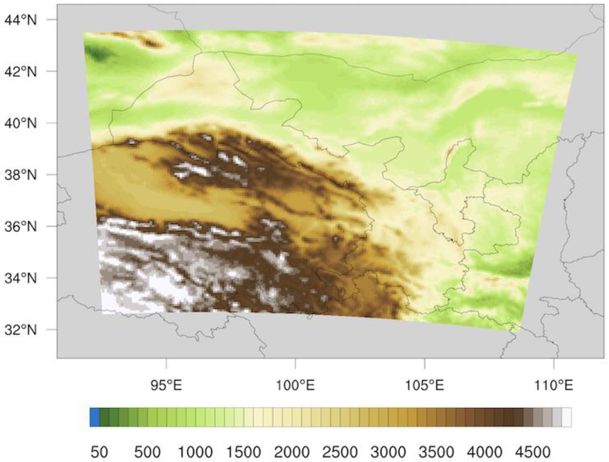
Figure 1. Digital elevation data of the single WRF domain with horizontal resolution at 8 km.
Preprints 68623 g001
Figure 2. One-month averaged CRPS and ensemble spread as a function of the forecast lead time from 10 to 54 hours wind speed forecast for the downscaling, BGM, and blending ensemble over 28 wind farms in Gansu, China.
Preprints 68623 g002
Figure 3. One-month averaged RMSE and MBE as a function of the forecast lead time from 10 to 54 hours wind speed forecast for the downscaling, BGM, and blending ensemble over 28 wind farms in Gansu, China.
Preprints 68623 g003
Figure 4. Rank histogram for wind forecast of the forecast lead time from 10 to 54 hours for the downscaling, BGM, and blending ensemble over 28 wind farms in Gansu, China.
Preprints 68623 g004
Table 1. Description of experiments including downscaling, BGM, and blending.
Experiment Initial Condition Perturbations Lateral Condition Perturbations
Downscaling Dynamical downscaling of ECMWF EPS ECMWF EPS
BGM WRF BGM ECMWF EPS
Blending Blending ECMWF EPS with WRF BGM ECMWF EPS
Table 2. RMSE and MBE of the ensemble mean for wind speed forecasts of the downscaling, BGM, and blending ensemble averaged over forecast lead time of 10 to 13 hours and 28 to 51 hours.
10 to 13 Hours 28 to 51 Hours
Downscaling BGM Blending Downscaling BGM Blending
RMSE 2.531 2.530 2.508 2.582 2.579 2.577
MBE 1.122 1.112 1.113 0.722 0.721 0.725
Disclaimer/Publisher’s Note: The statements, opinions and data contained in all publications are solely those of the individual author(s) and contributor(s) and not of MDPI and/or the editor(s). MDPI and/or the editor(s) disclaim responsibility for any injury to people or property resulting from any ideas, methods, instructions or products referred to in the content.
Copyright: This open access article is published under a Creative Commons CC BY 4.0 license, which permit the free download, distribution, and reuse, provided that the author and preprint are cited in any reuse.
Prerpints.org logo

Preprints.org is a free preprint server supported by MDPI in Basel, Switzerland.

Subscribe

© 2024 MDPI (Basel, Switzerland) unless otherwise stated