An Efficient Gaussian Mixture Model and Its Application to Neural Network

Preprint

Article

An Efficient Gaussian Mixture Model and Its Application to Neural Network

Altmetrics

Downloads

453

Views

190

Comments

Weiguo Lu

Deng Ding,Fengyan Wu,

Gangnan Yuan^*

Weiguo Lu

Deng Ding,Fengyan Wu,

Gangnan Yuan^*

This version is not peer-reviewed

Submitted:

06 August 2024

Posted:

13 August 2024

You are already at the latest version

Alerts

Abstract

Gaussian mixture models (GMMs) are powerful tools specifically suited for problems where data distributions are multi-modal. Inspired by Fourier expansion, we propose a concept called GMM expansion to approximate arbitrary densities. A simple learning method is introduced under this framework. Theoretical and numerical analyses are provided to show that densities under GMM expansion are able to approximate arbitrary densities with certain accuracy. The proposed learning algorithm demonstrates better accuracy and time efficiency compared to classic density approximation methods such as the Expectation Maximization (EM) algorithm and Bayesian variational inference (BVI) for Gaussian mixture models. The proposed framework also shows better accommodation of neural networks. Three neural network applications are built to demonstrate its usability. The accuracy of density estimation in neural networks is reported to be significantly improved in one of the applications. Another application shows that latent variables can be easily turned into random variables. This user-friendly method opens up more possibilities in terms of latent manipulation, embedding techniques, and many other potential uses.

Keywords:

Subject: Computer Science and Mathematics - Computer Science

1. Introduction

Gaussian Mixture Models (GMMs) are powerful, parametric, and flexible models in probabilistic modeling. In particular, GMMs address two important problems: the inverse problem and the uncertainity problem. The first, known as the inverse problem, arises when

f^{- 1} (x)

and x are not unique one-to-one mappings [23]. The second issue involves the uncertainty of both the data (aleatoric) and the model (epistemic) [4,5,6,7]. When considering these two problems together, the classic modeling assumption

y = f (x) + ϵ

becomes inadequate. In a probabilistic sense, this assumption is equivalent to

y \sim Normal (f (x), σ)

. However, to address the inverse and uncertainty problems, the model assumption should be

y \sim UnkownDistribution (θ (x))

. Under these conditions, when y no longer follows any known distribution, GMM become a viable option for modeling the data.

Fitting a GMM to observed data is related to two problems: determining the mixture components needed, and estimating the parameters of each mixture component. For the first problem, various techniques have been introduced [1]. For the second problem, the expectation maximization (EM) algorithm [11], developed as early as 1977, can fit GMMs by minimizing the negative log-likelihood (NLL). While the EM algorithm remains one of the most popular choices for learning GMMs [10,12,13], other methods have also been developed. However, the EM algorithm has some drawbacks. Srebro [16] raised an open question regarding the existence of local maxima between an arbitrary distribution and a GMM. This study also addressed the possibility that the Kullback-Leibler (KL) divergence between an arbitrary distribution and mixture models may have non-global local minima, especially when the target distribution has more than k components, but we fit it with a GMM with fewer than k components. AmÃ©ndola et al. [15] demonstrated that the likelihood function for GMMs is transcendental. Jin et al. [14] resolved the problem Srebro discovered and proved that with random initialization, the EM algorithm will converge to a bad critical point with high probability, and the local maxima can be arbitrarily worse than any global optimum. The maximum likelihood function is transcendental, resulting in multiple critical points. Because of the problems related to likelihood functions, some methods, such as the Wasserstein distance, have been explored. Wasserstein distances are presented to replace the NLL function, which minimizes either the KL divergence or the NLL function [10,17,18]. These methods avoid the disadvantage of using NLL; however, the calculation and formulation of the learning process are relatively complex. Another state-of-the-art method is Bayesian variational inference (BVI) for a Gaussian mixture model [33,35,37]. This method applies Bayesian techniques and variational inference to the Gaussian mixture model. Practically, this method avoids the singularity problems in EM; however, many priors are required in the inference algorithms. When these priors are mismatched, the algorithmâs performance may be less accurate than EM.

Instead of following the EM and BVI, we adopt a different path. One of the main contributions of this study is the concept of GMM expansion, which is based on the idea of Fourier expansion applied to density approximations. Like Fourier expansion, we process that any density can be approximated by a linear combination of a set of Gaussian distributions. If this argument is valid, the Gaussian distributions in the GMM become the basis, similar to the cosine and sine functions in Fourier expansions. Some studies show that all normal mixture densities are dense in the set of all density functions under the

L^{1}

metric [1,2,3,34], and the mixture densities are dense in the set of all density functions under the Wasserstein metric. In this study, we further prove that mixture densities built under the GMM expansion can approximate an arbitrary density with a certain accuracy. Numerical analysis was also conducted to secure the usability of the GMM expansion in practice.

In GMM expansion, the Gaussian distributions act as "basis functions" that do not require additional parameterization. The only parameter that needs to be learned is

π

. These "basis functions" represent how much detail our models are able to capture. The benefit of this idea is that learning on a predetermined basis becomes relatively simple. A simple algorithm without heavy formulation is proposed for density approximation under the GMM expansion. We show that our method can be more accurate, faster, and easier to use compared to state-of-the-art methods such as EMs and BVI.

GMMs have been used in computer vision and pattern classification, among many other fields [10,19,20,21,22]. Another significant benefit of the proposed method is that the GMM expansion can improve the integration of GMM in neural networks. The proposed method has no singularity issue compared to EM, which significantly improves performance when a neural network is trained to predict a distribution. The simplicity of the proposed method also allows us to easily utilize GMM into neural networks to manipulate the latent space. We built three applications to demonstrate the benefits that GMM can bring to neural networks.

Section 2 introduces the GMM expansion method, which proves that GMM expansion can approximates arbitrary densities, learning algorithms, and convergence. Section 3 provides our numerical experiments and a comparison with state-of-the-art density learning methods. Section 4 presents three neural-network applications that demonstrate the integration of the proposed method into a neural network. The final section provides a summary and conclusions.

2. GMM Expansion

In this section, we provide a detailed description of the principle of the GMM expansion using learning algorithms. Theoretical and numerical analyses were conducted to prove that the GMM expansion can approximate arbitrary densities with a bounded error. Gaussian mixture models in the high-dimensional case are theoretically possible; however, similar to the Fourier expansion method, the complexity of the algorithm for GMM grows exponentially with the number of dimensions. Due to arithmetic constraints, we will discuss higher dimensions in future work. In this study, we conducted experiments in one and two dimensions.

2.1. The Concept of GMM Expansion

The idea behind the GMM decomposition is akin to a Fourier series in probability, where an arbitrary density can be approximately decomposed by an infinite mixture of Gaussian distributions. As aforementioned, several studies have proven that the likelihood of a GMM has numerous critical points. There are multiple sets of

π, μ

and

σ

that can produce the same likelihood result on a particular dataset. If we consider that GMM can decompose any density like the Fourier series decomposes into a periodic sequence, we can hold

μ

and

σ

unchanged and focus on finding the optimal solution for

π

. Based on this concept, the setup of the GMM expansion is as follows:

Observation X follows an unknown distribution with density $f (x)$ ;
$g (x) = \sum_{N} π_{i} ϕ_{i} (x)$ is the density of GMM;
$\sum_{N} π_{i} = 1$ ;
$ϕ_{i} (x)$ is the i-th normal distribution with mean $μ_{i}$ and standard deviation $σ$ ;
define $r = \frac{\max (X) - \min (X)}{n}$ as the interval for locating $μ_{i}$ ;
$μ_{i} = \min (X) + i \times r$ ;
$σ$ is a hyperparameter and the same for all Gaussian components, usually $r \leq σ \leq 5 r$ .

The

μ

and

σ

of the component distributions are non-parametric and do not need to be optimized. The parameter

π

is the only remaining problem for us to solve. There are justification

σ

as a hyper-parameter, which we will further demonstrate in the next subsection. From the above settings, to ensure this system works, the GMM expansion must satisfy one condition: for any

f (x)

, there exists a

g (x)

such that

∣ f (x) - g (x) ∣ < ϵ

. In the next subsection, we will prove that this is indeed the case.

2.2. Approximate Arbitrary Density by GMM Expansion

First, we would like to introduce a Lemma from Villani’s book [34].

Lemma 1

[34] Let

X

be a complete separable metric space and

P \in (0, \infty)

. Then the Wasserstein space

P_{p} (X)

, metrized by the Wasserstein distance

W_{p}

, is also a complete separable metric space. i.e. any probability measure can be approximated by a sequence of probability measures with finite support.

The proof of this Lemma is given by Theorem 6.18 in [34]. Under this Lemma, the Dirac measure, which can be seen as a degenerate GMM, is able to approximate any arbitrary distribution with arbitrary precision in the Wasserstein space. To further elaborate on this, when the Gaussians are very close to degeneration, which is close to the Dirac measure, we have the following numerical interpretation of Lemma 1 under the GMM expansion setting.

Consider a fine enough partition based on

μ

over the support of the probability measure such that

ω_{i} = (μ_{i} - r, μ_{i} + r]

, then we have:

[\begin{matrix} \int_{ω_{0}} ϕ_{0} (x) d x & . & . & . \int_{ω_{0}} ϕ_{n} (x) d x \\ ⋮ & ⋮ & ⋮ & ⋮ \\ \int_{ω_{N}} ϕ_{0} (x) d x & . & . & . \int_{ω_{N}} ϕ_{n} (x) d x \end{matrix}] [\begin{matrix} π_{0} \\ ⋮ \\ π_{N} \end{matrix}] = [\begin{matrix} P_{g} \{ω_{0}\} \\ ⋮ \\ P_{g} \{ω_{N}\} \end{matrix}] .

\int_{ω_{i}} ϕ_{i} (x) d x \approx 1

, indicating that each Gaussian component is very dense in its region, the GMM becomes a discrete distribution that can precisely map the estimated probability mass. It becomes:

[\begin{matrix} 1 & . & . & . 0 \\ ⋮ & ⋮ & ⋮ & ⋮ \\ 0 & . & . & . 1 \end{matrix}] [\begin{matrix} π_{0} \\ ⋮ \\ π_{N} \end{matrix}] \approx [\begin{matrix} P_{g} \{ω_{0}\} \\ ⋮ \\ P_{g} \{ω_{N}\} \end{matrix}]

[\begin{matrix} P_{g} \{ω_{0}\} \\ ⋮ \\ P_{g} \{ω_{N}\} \end{matrix}] \approx [\begin{matrix} π_{0} \\ ⋮ \\ π_{N} \end{matrix}] = [\begin{matrix} P_{f} \{ω_{0}\} \\ ⋮ \\ P_{f} \{ω_{N}\} \end{matrix}]

(1)

where

P_{g}

is the density function for the GMM and

P_{f}

is the target density function. These simple deductions, together with Lemma 1 show that any probability measure can also be approximated by probability measures constructed by the GMM.

Theorem 2.

For any probability density

f (x)

and a given error e, we can find a Gaussian mixture

g (x)

to approximate it. Proof Let

f (x)

be a piecewise continuous density function, whose integral over a finite interval

[a, b]

\begin{matrix} \int_{a}^{b} f (x) d x = 1 - ϵ, ϵ > 0 . \end{matrix}

(2)

We consider a sequence

a = x_{1} < x_{2} < \dots < x_{N - 1} < x_{N} = b

such that

f (x)

is continuous in every interval

[x_{i}, x_{i + 1}]

for

x_{i} \leq x < x_{i + 1}

and

i = 1, 2, \dots, N - 1

. When the partitioning is sufficiently fine, continuous function

f (x)

on a bounded interval

[x_{i}, x_{i + 1}]

is bounded and there exist a constant

ξ_{i}

such that

\begin{matrix} | f (x_{i}) (x_{i + 1} - x_{i}) - \int_{x_{i}}^{x_{i + 1}} f (x) d x | < ξ_{i} . \end{matrix}

(3)

The error of two functions under one norm is

\begin{matrix} \sum_{i = 1}^{N} | f (x_{i}) (x_{i + 1} - x_{i}) - \int_{x_{i}}^{x_{i + 1}} f (x) d x | < \sum_{i = 1}^{N} ξ_{i}, \end{matrix}

(4)

and

\begin{matrix} | \sum_{i = 1}^{N} f (x_{i}) (x_{i + 1} - x_{i}) - \int_{a}^{b} f (x) d x | \end{matrix}

(5)

\begin{matrix} \leq \sum_{i = 1}^{N} | f (x_{i}) (x_{i + 1} - x_{i}) - \int_{x_{i}}^{x_{i + 1}} f (x) d x | . \end{matrix}

(6)

There exists a sufficiently large

\hat{N}

such that when

N > \hat{N}

, for any

ξ

\begin{matrix} \sum_{i = 1}^{N} | f (x_{i}) (x_{i + 1} - x_{i}) - \int_{x_{i}}^{x_{i + 1}} f (x) d x | < \sum_{i = 1}^{N} ξ_{i} < ξ . \end{matrix}

(7)

According to Lemma 1, the first term of Equation (6) can be approximated with an arbitrary precision using a finite combination of Dirac measures. We assume that the error between the Gaussian components

Φ_{i} (x)

and the Dirac measure

δ (x)

within each interval is

e_{i}

in one norm.

\begin{matrix} f (x_{i}) (x_{i + 1} - x_{i}) \approx α_{i} δ (x; [x_{i}, x_{i + 1}]) \approx α_{i} Φ_{i} (x) \end{matrix}

(8)

where

0 \leq α_{i} \leq 1, \sum α_{i} \approx 1

The global error can be shown as

\begin{matrix} \begin{matrix} \sum_{i = 1}^{N} | α_{i} Φ (x; [x_{i}, x_{i + 1}], σ) - \int_{x_{i}}^{x_{i + 1}} f (x) d x | \\ = \sum_{i = 1}^{N} | α_{i} Φ (x; [x_{i}, x_{i + 1}], σ) - f (x_{i}) (x_{i + 1} - x_{i}) \\ + f (x_{i}) (x_{i + 1} - x_{i}) - \int_{x_{i}}^{x_{i + 1}} f (x) d x | \\ \leq \sum_{i = 1}^{N} | α_{i} Φ_{i} (x; [x_{i}, x_{i + 1}], σ) - f (x_{i}) (x_{i + 1} - x_{i}) | \\ + \sum_{i = 1}^{N} | f (x_{i}) (x_{i + 1} - x_{i}) - \int_{x_{i}}^{x_{i + 1}} f (x) d x | \\ < \sum_{i = 1}^{N} e_{i} + \sum_{i = 1}^{N} ξ_{i} \\ < \sum_{i = 1}^{N} e_{i} + ξ \end{matrix} \end{matrix}

(9)

and

\begin{matrix} | \sum_{i = 1}^{N} α_{i} Φ_{i} (x; [a, b], σ) - \int_{- \infty}^{\infty} f (x) d x | < \sum_{i = 1}^{N} e_{i} + ξ + ϵ = e . \end{matrix}

(10)

where

\sum_{i = 1}^{N} α_{i} Φ_{i} (x; [a, b], σ)

is a mixture of Gaussian.

Remark 1

Despite the introduction of multiple error terms in the above approximation, the global error can be controlled, and the results of the numerical experiments support this conclusion. The GMM expansion, as a special kind of Gaussian mixture model, also satisfies the above theorem, and an example is given in the Appendix A.

2.3. Total Variation Distance Analysis For Small Region

Even though GMMs can approximate arbitrary densities similar to frequency distributions under Wasserstein metrics, the density within a fine region remains undiscussed. In other words, even if we learn a model where the probability mass is equal to the target density

P_{g} \{ω\} = P_{f} \{ω\}

, the differentiation might not be equal

\frac{d P_{g} \{ω\}}{d x} \neq \frac{d P_{f} \{ω\}}{d x}

. To further analyze the difference in probability density in fine regions, we introduce the well-known total variation distance.

Assuming we have learned a Gaussian mixture density g that correctly maps to the target distribution fand considering the same partition as shown in Section 2.2, let Equation (1) be satisfied. The total variation distance (TVD) based on the partition

ω

is given by

T V D = \frac{1}{2} \sum_{i = 1}^{n} \int_{ω_{i}} | f (x) - g (x) | d x .

Because the integration is difficult to calculate, we divide

ω_{i}

further into m smaller regions to estimate TVD:

\sum_{k = 1}^{m} d_{k} = ω_{i},

\begin{matrix} T V D & \approx \frac{1}{2} \sum_{i = 1}^{n} \sum_{j = 1}^{m} \int_{d_{i j}} | f (x) - g (x) | d x \\ \approx \frac{1}{2} \sum_{i = 1}^{n} \sum_{j = 1}^{m} | P_{f} \{d_{i j}\} - P_{g} \{d_{i j}\} | . \end{matrix}

Denote that

L (ω_{i}) = \frac{1}{2} \sum_{j = 1}^{m} | P_{f} \{d_{i j}\} - P_{g} \{d_{i j}\} | .

(11)

Here

L (ω_{i})

is the discrete approximation of TVD within region

ω_{i}

. If

L (ω_{i})

is universally bounded in some conditions for all

ω

, the overall TVD is bounded. For any

x_{i j}

from

ω_{i}

, if

| P_{f} \{x_{i j} \pm d\} - P_{g} \{x_{i j} \pm d\} | \leq τ_{i} \leq τ,

we obtain

T V D \leq n * m * τ .

Remark 2 In the Appendix B, we illustrate why TVD is controllable and

L (ω_{i})

is universally bounded under certain conditions. The experiments described in Section 3 verify this result.

2.4. Learning Algorithm and Convergence

From Section 2.1 to Section 2.3, we draw the following conclusion: The parameter

π

s are proportional to the distribution of data, resulting in a simple update for the learning algorithm. The whole algorithm can be demonstrated as follows.

Algorithm 1:GMM Expansion

Initialization

Calculate r based on the number of Gaussian components n, $r = \frac{Max (X) - Min (X)}{n}$ .
Evenly spread $μ = [μ_{1}, μ_{2}, \dots, μ_{n}]$ across $Max (X)$ and $Min (X)$ , so that $μ_{i + 1} - μ_{i} = r$ .
Define hyperparameter $σ$ with respect to r, e.g., $σ = r$ , $σ = 3 r$ , etc.
Define hyperparameter d with respect to $σ$ , e.g., $d = σ / 4$ , $d = σ / 6$ , etc.
Define a constant $α = β (P (μ_{i} \pm \frac{d}{2}) - P (μ_{i} - \frac{r}{2} \leq x \leq μ_{i} - \frac{r}{2} + d))$ .
Initialize $π_{1} = π_{2} = \dots = π_{N} = \frac{1}{N}$ .

Update Procedure

1:: for each $x_{d}$ do
2:: $j = argmin (∣ x_{d} - μ ∣)$
3:: $π_{j}^{+ 1} = π_{j} + α$
4:: end for

Finally, re-normalize

π

s to ensure

\sum π_{i} = 1

Since we always seek to maximize the likelihood, a gradient ascent method should be applied. The derivative of the i-th

π

with respect to

g (x_{d})

for each observation partially reveals the methodology of the proposed algorithm:

\frac{\partial g (x_{d})}{\partial π_{i}} = ϕ_{i} (x_{d}) .

(12)

Because

μ

, and

σ

are not longer parameters, the gradient direction from every single data point is always positive, which is directly related to

ϕ

. After learning from the whole dataset, the final step is re-normalization to ensure

\sum π_{i} = 1

. Figure 2 illustrates the learning process. The parameter

σ

is regarded as a hyperparameter that controls the smoothness of the GMM. More details are provided in Appendix B. The parameter

α

is a proportional hyper-parameter designed based on the proof shown in Section 2.1, Section 2.2 and Section 2.3. The parameter

β

is the learning rate, similar to any gradient ascend method. The probability part of

α

can be referred to in Eq. A7, where P is the probability of a normal distribution. The reasoning is provided in the Appendix B and illustrated in Figure 2. Considering a data point, the algorithm adjusts the probability with respect to

π

while maintaining the rest of the density in proportion. Further explanation is provided in the convergence analysis. The proposed algorithm is simple yet efficient; it processes each data point in the dataset only once. On the contrary, EM and BVI algorithms require several iterations over the dataset to converge.

Moving on to the discussion of the convergence, consider that we have a set of bases Gaussian components

{\{ϕ_{i} (x)\}}_{n}

. According to Theorem 6.18, the mixture densities are dense and can approximate any Dirac mass with arbitrary precision under the Wasserstein distance. Dirac masses can be considered a degeneration of the Gaussian distribution. Assuming the Gaussian components are sufficiently dense, for any sample data point

x_{d}

, we can find a Gaussian component very close to it, such that

ϕ (x_{d}; μ_{d}, σ) \approx ϕ (μ_{d}; μ_{d}, σ)

. This means:

\begin{matrix} g (x_{d}) = \sum_{i}^{N} π_{i} ϕ_{i} (x_{d}) \approx π_{d} ϕ_{d} (x_{d}) \approx π_{d} ϕ_{d} (μ_{d}), \end{matrix}

(13)

\begin{matrix} ϕ_{d} (μ_{d}) = a, g (x_{d}) \approx a π_{d}, \end{matrix}

(14)

where a is a constant. Similar to BVI and the EM algorithm, the proof of convergence and the algorithm both rely on a binary latent variable Z[33,35,36]. In this context, we assume

γ

is a binary latent variable, which indicates that observation

x_{d}

is sampled from the n-th mixture component. This ensures that the density function is expected as:

\begin{matrix} p (x | γ) = \prod_{n = 1}^{N} ϕ {(x | μ_{n}, σ)}^{γ}, \end{matrix}

(15)

We can observe the connection between the assumptions we based on the analyses provided in [34] and the latent variable model used in BVI and EM. This indicates that Eq.(13)is equivalent to Eq.(15). Thus, we will pursue a similar approach by considering a variable

Z \in N = {\{z_{n}\}}_{N}

\begin{matrix} z_{i} = \sum_{d = 1}^{D} γ_{d i}, \\ \sum_{i = 1}^{N} z_{i} = D, \\ γ_{d i} = \{\begin{matrix} 1 & i = argmin (x_{d} - μ) \\ 0 & otherwise \end{matrix} \end{matrix}

The log-likelihood function

log (L)

is:

\begin{matrix} log (L) = \sum_{d}^{D} log (\sum_{i}^{N} π_{i} ϕ_{i} (x_{d})), \\ = \sum_{d}^{D} log (\sum_{i}^{N} γ_{d i} π_{i} ϕ_{i} (x_{d})), \\ = \sum_{d}^{D} \sum_{i}^{N} γ_{d i} log (π_{i} ϕ_{i} (x_{d})), \\ = \sum_{i}^{N} \sum_{d}^{D} γ_{d i} log (π_{i} ϕ_{i} (x_{d})), \\ log (L) \approx \sum_{i}^{N} z_{i} log (a π_{i}) . \end{matrix}

Define a function with the Lagrange multiplier :

\begin{matrix} A = \sum_{i}^{N} z_{i} log (a π_{i}) + λ (1 - \sum_{i}^{N} π_{i}) \end{matrix}

\begin{matrix} \frac{\partial A}{\partial π_{i}} = z_{i} \frac{1}{π_{i}} - λ = 0, \\ Set λ = D, then π_{i}^{*} = \frac{z_{i}}{D} \end{matrix}

From Algorithm 1, denote

π^{a l g}

is the

π

learned from the proposed algorithm. After running the update procedure, we obtain:

\begin{matrix} π_{i}^{a l g} = \frac{\frac{1}{N} + z_{i} α}{\sum_{i}^{N} \frac{1}{N} + z_{i} α} = \frac{\frac{1}{N} + z_{i} α}{1 + D α}, \end{matrix}

when N and

D α

are sufficiently large,

\begin{matrix} π_{i}^{a l g} \approx π^{*}, \end{matrix}

Based on the above assumption, our method is equivalent to the statistic of the frequency distribution.

\begin{matrix} g (x_{d} | π) = \sum_{i} \frac{1}{N} ϕ (x_{d}) \approx \frac{1}{N} ϕ_{k} (x_{d}) \\ g (x_{d} | π^{*}) = \sum_{i} \frac{z_{i}}{D} ϕ (x_{d}) \geq \frac{z_{k}}{D} ϕ_{k} (x_{d}) \\ z_{i} \geq 1, D \leq N, k = argmin (x_{d} - μ), \end{matrix}

For every data point

x_{d}

\begin{matrix} g (x_{d} | π^{*}) > g (x_{d} | π), \\ Likelihood L (X | π^{a l g}) \approx L (X | π^{*}) \geq L (X | π) \end{matrix}

The proposed algorithm can employ both

π^{a l g}

and

π^{*}

for approximation.

π^{a l g}

is ideal for situations with a small number of data points where a conservative approximation for unseen regions is required. On the other hand,

π^{*}

is more suitable when a closer approximation to the dataset is needed.

3. Numerical Experiments

In this section, we demonstrate the effectiveness of the proposed GMM expansion and learning algorithm. Section 3.1 presents experiments that illustrate and discuss the fundamentals of the proposed method for approximating arbitrary densities. For usability, Section 3.2 provides comparative studies, contrasting the proposed method with state-of-the-art techniques such as BVI and EM algorithm. These comparisons highlight the advantages of the proposed method.

3.1. Density Approximation

The GMM expansion aims to approximate densities without relying on the specific form of the target distributions. Figure 1 shows cases of two density approximation. The left side of Figure 1 displays the target densities, while the right side shows these target densities alongside their approximations using our GMM method. In the upper plot, the target density is a mixture of continuous and smooth distributions, using five normal distributions. The lower plot features a target distribution that combines normal, T, and uniform distributions.

In terms of approximation accuracy, the proposed method performed exceptionally well for both the smooth and non-smooth cases. The overall and most crucial features of the target densities were well-preserved, although some details of non-smooth densities were difficult to recover. Considering that the Gaussian distributions are inherently smooth, we expected the GMM to perform better when approximating smooth target densities. Geometrically, when target distributions consist of components with bell-shaped structures, GMM is a particularly suitable choice for approximation. However, in cases like the target distribution in the lower plot, which includes a uniform distribution among its components, GMM may struggle to capture fine details unless a sufficiently large number of components are used. According to the GMM expansion idea, GMM is expected to capture finer structures, such as deep cuts and straight lines, with a larger set of basis components. This expectation is consistent with the theoretical proof provided in Section 2. As long as GMM captures most of the critical features with a certain level of accuracy, the approximation can be considered good. Further numerical justification is provided later in this section. Further numerical justification is provided later in this section.

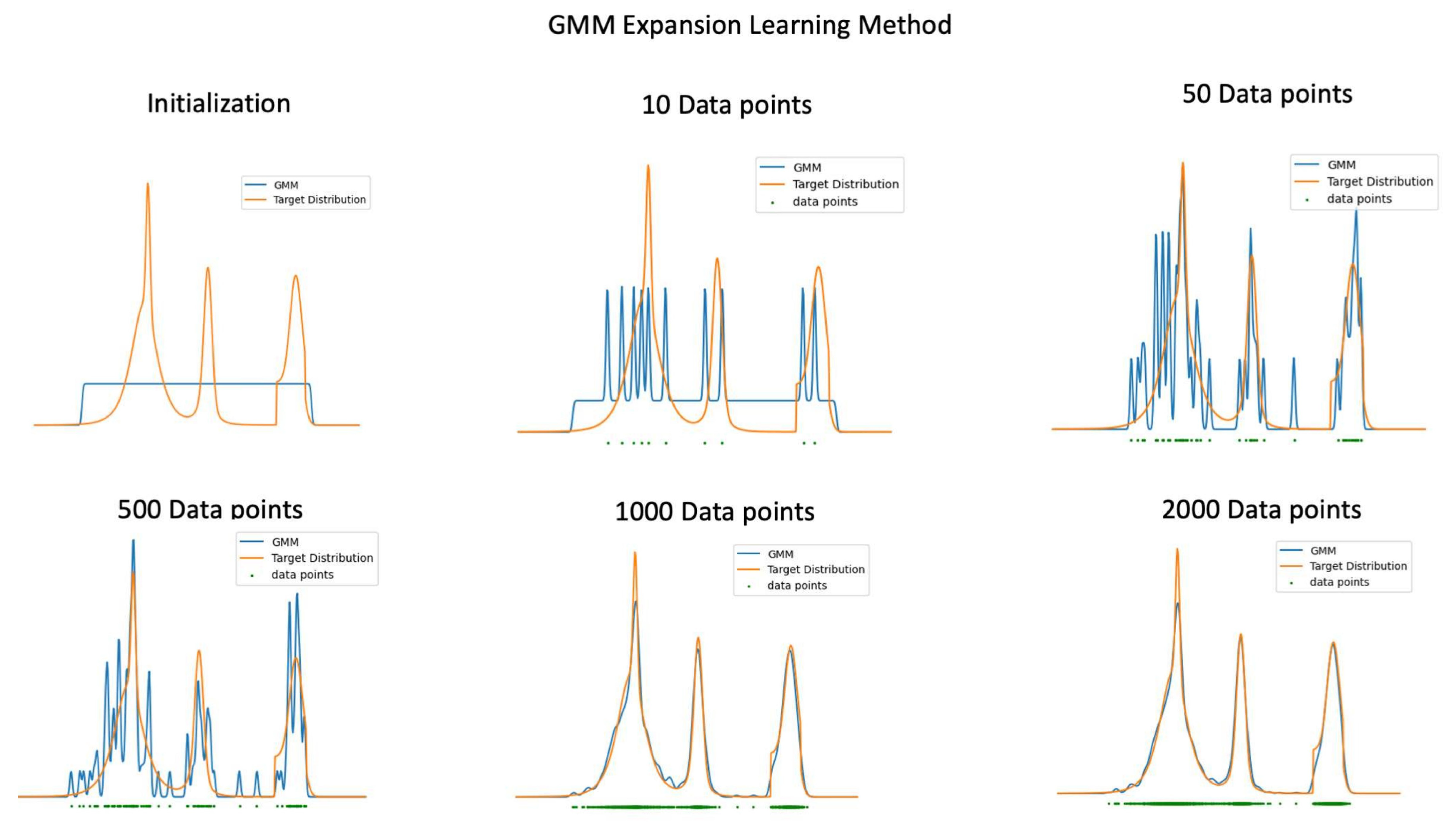
The learning process is illustrated in Figure 2. Initially, the density of our GMM closely resembles a uniform distribution before training. As the training progresses and the dataset is processed, the density gradually conforms to the original target density. Given that the base distributions are fine and dense, we can achieve a good approximation without needing to learn the parameters

μ

and

σ

for each Gaussian distribution. Unlike traditional methods where GMM requires learning

π

μ

and

σ

, fixing

μ

and

σ

as bases and smoothness, especially in neural network, which we will present in section 4 adjusting the density through

π

offers advantages, particularly in neural network applications, as discussed in Section 4. Additional approximation examples are shown in Appendix Figure A5.

After graphically demonstrating the GMM expansion and learning algorithm, a quantitative study was conducted to further discuss the properties of the proposed method. In these experiments, the total variance distance(TVD) from Section 2 was applied. Since

μ

was predetermined, TVD is denoted as L and is calculated as follows.

\begin{matrix} 2 L = & | P_{t a r g e t} \{x \leq μ_{1} - d\} - P_{g m m} \{x \leq μ_{1} - d\} | \\ + \sum_{i = 1}^{n} | P_{t a r g e t} \{μ_{i} \pm d\} - P_{g m m} \{μ_{i} \pm d\} | \\ + | P_{t a r g e t} \{x > μ_{N} + d\} - P_{g m m} \{x > μ_{N} + d\} | . \end{matrix}

(16)

Measuring the estimation accuracy using Equation (16) has several advantages. First, it is easy to calculate. Second, even without the target density in its current form, we can still compute the loss using a discrete statistical estimation. The minimum and maximum values of the loss, which were

[0, 2]

, are clearly evident. Evidence is provided below.

\begin{matrix} 2 L & \leq | P_{t a r g e t} \{x \leq μ_{1} - d\} - 0 | + \sum_{i = 1}^{n} | P_{t a r g e t} \{μ_{i} \pm d\} - 0 | \\ + | P_{t a r g e t} \{x > μ_{N} + d\} - 0 | + | 0 - P_{g m m} \{x \leq μ_{1} - d\} | \\ + \sum_{i = 1}^{n} | 0 - P_{g m m} \{μ_{i} \pm d\} | + | 0 - P_{g m m} \{x > μ_{N} + d\} | . \end{matrix}

That means

0 \leq L \leq 1

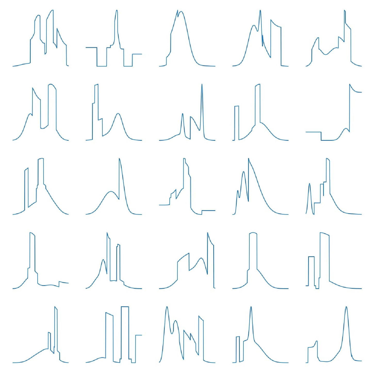
In this quantitative study, the proposed method was used to approximate two sets of randomly generated distributions, calculating the average TVD using Equation (16) between the target distribution and the approximated GMM. Table 1 and Table 2 present the results of using our method to learn two types of distributions. Similar to Figure 1, the target distributions in Table 1 are randomly generated Gaussian mixture distributions. We sampled 5000 data points for learning and used GMM with 200 components for learning. More approximation examples are shown in Appendix Figure A5 subplots (1)–(3). Table 2 presents the results of approximating target distributions containing Normal, T, and uniform distributions, with examples shown in Appendix Figure A5 subplots (4)–(6). Since

0 \leq L \leq 1

, the average L for both types of distributions are less than

0.1

. This indicates that approximation error is considerably low, with the margin of error for our experiments being less than

5 %

. In the later part of the section, we present a direct comparison with other methods. The results also indicate that the GMM generally performs better in approximating smooth target densities. Another important factor in the algorithm is the hyperparameter

σ

. Table 1 and Table 2 show how changes in

σ

affect the accuracy of the algorithm. The approximation accuracy benefits from a slightly larger

σ

for smooth densities, but a smaller

σ

works better for non-smooth densities. However, the overall improvement in L function was less than

0.02

, indicating that the benefits are not significant. This result supports treating

σ

as a hyperparameter. Depending on the situation,

σ

can be set smaller (e.g.,

1 * r

) if a closer match to the original dataset is required or larger (e.g.,

3 * r

) for smoother distributions.

The above experiment discusses approximation accuracy with the same component distribution sizes but varying

σ

. It is important to address how the sizes of the component distributions and the dataset affect the approximation accuracy. The experimental results shown in Table 3 demonstrates the performance of the proposed method under various setups. Similar to the experiments in Table 2 and Table 1, the average L over approximations of 30 different randomly generated mixture densities was calculated. A GMM with component sizes ranging from 10 to 1000 was tested. Table 1, Table 2, and Table 3 show how increasing the data size from 5,000 to 50,000 affects approximation accuracy. The findings indicate that the proposed method benefits from a large dataset. Results from Table 1 and Table 2 show that with 5,000 data points and 200 components, the approximation accuracy was improved from 0.04369 to 0.01475 when the data size increased to 20,000. Further increasing the number of data points to 50,000, provided only a slight additional benefit. Table 3 indicates increasing the component size from 10 to 200 delivers significant improvements. However, increasing the component size to 500 and 1000 does not necessarily result in better performance. An approximation with 500 components and 50,000 data points achieved the best accuracy with

L = 0.0101

, but the improvement over 200 components (

L = 0.0125

) was minimal. These findings align with our intuitive understanding of GMM expansion, confirming that a certain number of basis components is necessary to ensure a good approximation. Increasing data points and components helps capture finer details, but determining the optimal number of components relative to the dataset size lacks a clear formula. Nonetheless, our experiments show that the proposed method is robust with 200 components.

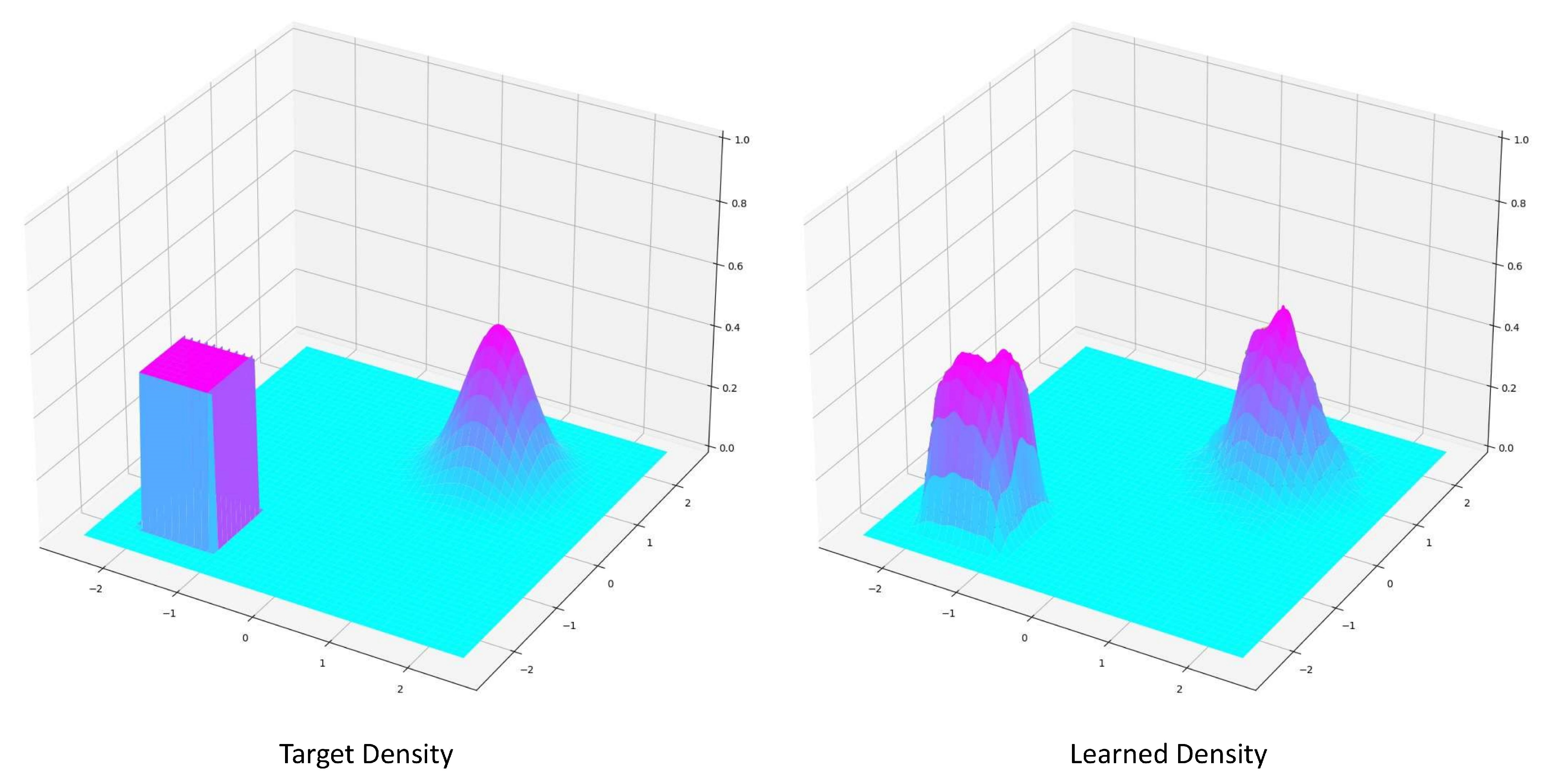
The aforementioned experiments were conducted using one-dimensional settings. The proposed method as also applicable in high-dimensional cases. A two dimensional example is shown in Figure 3. In Fourier expansion, increasing dimensions exponentially enlarges the size of the base frequency components. The proposed method faces a similar problem, managing higher-dimensions requires more bases to capture inter-dimensional correlations. To address this, clustering methods such as K-means are used with the EM algorithm, where cluster sizes are predetermined. The BVI method attempts to solve this problem by optimizing the posterior distribution through techniques like mean-field approximation or Markov chain monte-carlo (MCMC). However, these methods each have limitations. For example, the EM algorithm can suffer from singularities, and the BVI approach requires prior and posterior distributions, which introduces implicit biases. Higher-dimensional density estimation is more complex compared to existing methods due to the correlation between dimensions. We plan to further develop this method and discuss future work. In the next subsection, we will directly compare the proposed method with state-of-the-art distribution approximation techniques, particularly EM and BVI.

3.2. Comparison Study

EM and BVI are state-of-the-art density approximation methods [33,35,37]. Scikit-learn1 provides a well-built Python package for implementing these methods, alongwith detailed explanation and summaries. In this subsection, we compare our proposed method with EM and BVI. The algorithms for both the EM and BVI were obtained from Scikit-learn.

Figure 4. Experiment Density Set

The comprehensive performance comparison results for the proposed method, EM, and BVI are presented in Table 4. Accuracy and training time were compared, with all values presented as mean and standard deviation. Two variations of the EM algorithm were tested: EM K-means, which initializes parameters using the K-means methods, and EM-Random, which uses randomly selected data points. Similar to the experiments in Table 1, Table 2, and Table 3, a set of mixture distributions was randomly generated as illustrated in Figure 4. For each mixture distribution, 2000 data points were sampled for training. The component sizes ranged from 20 to 1000. We used the Total Variation Distance (TVD) to evaluate approximation accuracy. Since the cumulative density function is not provided in Scikit-learn, we estimated the TVD using a slightly modified approach. The equation for this estimation is as follows:

L = \frac{1}{2} \sum_{d} ∣ f_{g m m} (x_{d}) - f_{t a r g e t} (x_{d}) ∣ ▵ x_{d}

This causes the result in Table 4 be slightly different from the results in Table 1, Table 2, and Table 3

This experiment demonstrates that the proposed method is superior to both EM and BVI. Our method, with a component size of 200, had the lowest TVD as well as the lowest training time compared to the other methods. Various factors and fundamentals can cause the EMs and BVI to underperform when the number of Gaussians increases. We consider one of the most important factor is

σ

. How we handle

σ

is also the most notable difference between our method and others. Learning

σ

throughout the training process can cause degeneration. When there are insufficiently many points for a mixture components,

σ

may tend toward zero and infinite likelihood may occur or the mixture component may fall into singularity. This requires artificial regularization of the covariance and causes instability when applying the GMM in other models, such as neural networks. In the next section, we describe four applications that demonstrate how a neural network can benefit from the proposed method.

4. Neural Network Application

In this section, three neural network applications are designed to demonstrate how the GMM expansion and proposed learning algorithm can be integrated into neural networks to deliver various functionalities. The first application shows how the model performance can be enhanced when learning probabilistic outputs. The second and third applications utilize the proposed method to transform latent variables into random variables. In the second application, latent variables in an Auto-encoder [25] are converted into random variables modeled as GMM distributions. In the third application, the Gram matrices in the style transfer algorithm [9] are presented as Gram matrix distributions. In addition to the experimental results in this section, additional experiment results are given in Appendix C.

4.1. Probabilistic Output

Generally, data is not normally distributed, which makes modeling with

f (x) = y + ϵ

inadequate. One solution is to introduce a Gaussian Mixture Model (GMM) to predict the distribution for each input, so

f (x) = G M M (π, μ, σ)

. This approach addresses the issue where x and y are not unique one-to-one mappings. Tensorflow-probability2 provides a well-built package and examples to demonstrate how to implement GMM in a neural network. However, training to predict GMM parameters can be difficult. Specifically, the singularity problem may arise, as mentioned in earlier Section 3. To put it simply,

σ

can approach zero during training. Probabilistic models are usually trained with likelihood functions, and when

σ

tend toward zero, it can lead to infinite likelihoods, causing the cost function to explode. By applying GMM expansion, we can solve this problem and achieve better learning outcomes.

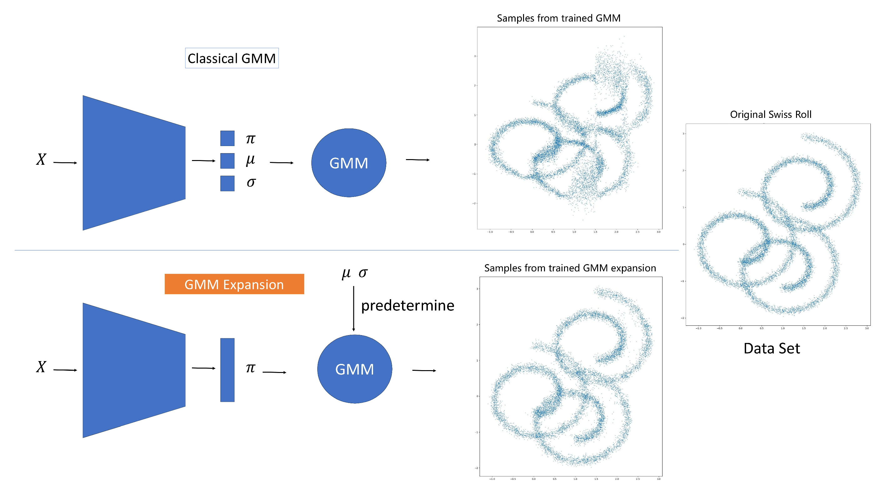
Figure 5 illustrates this concept. The classic Swiss roll data exemplify the non-unique mapping of x and y. By introducing some shifts and variance, we obtain the dataset shown on the right side of Figure 5. The upper plot shows the learning results using the standard GMM approach provided by Tensorflow-probability. In this method, the neural network is trained to output

π, μ, σ

to form a GMM for each prediction. The lower plot shows the results of our approach. By fixing

μ

and

σ

as constants, our GMM expansion only requires a set of

π

to form the GMM. The neural network in our method is trained to predict a set of

π

. The same likelihood function is used for training and no singularity problem should be addressed. The results are evident: the predictions from our model are visually and significantly better than those from the standard approach. In this experiment, both models are treated equally, using the same multilayer perceptron with identical hidden layer sizes and training steps. Notably, the proposed learning algorithm can also be used to preprocess data into

π

s. Training from the likelihood of GMM transforms into the likelihood of the discrete distribution

π

, which is known as entropy.

4.2. Mnist Data Set of Handwritten Digits Generation

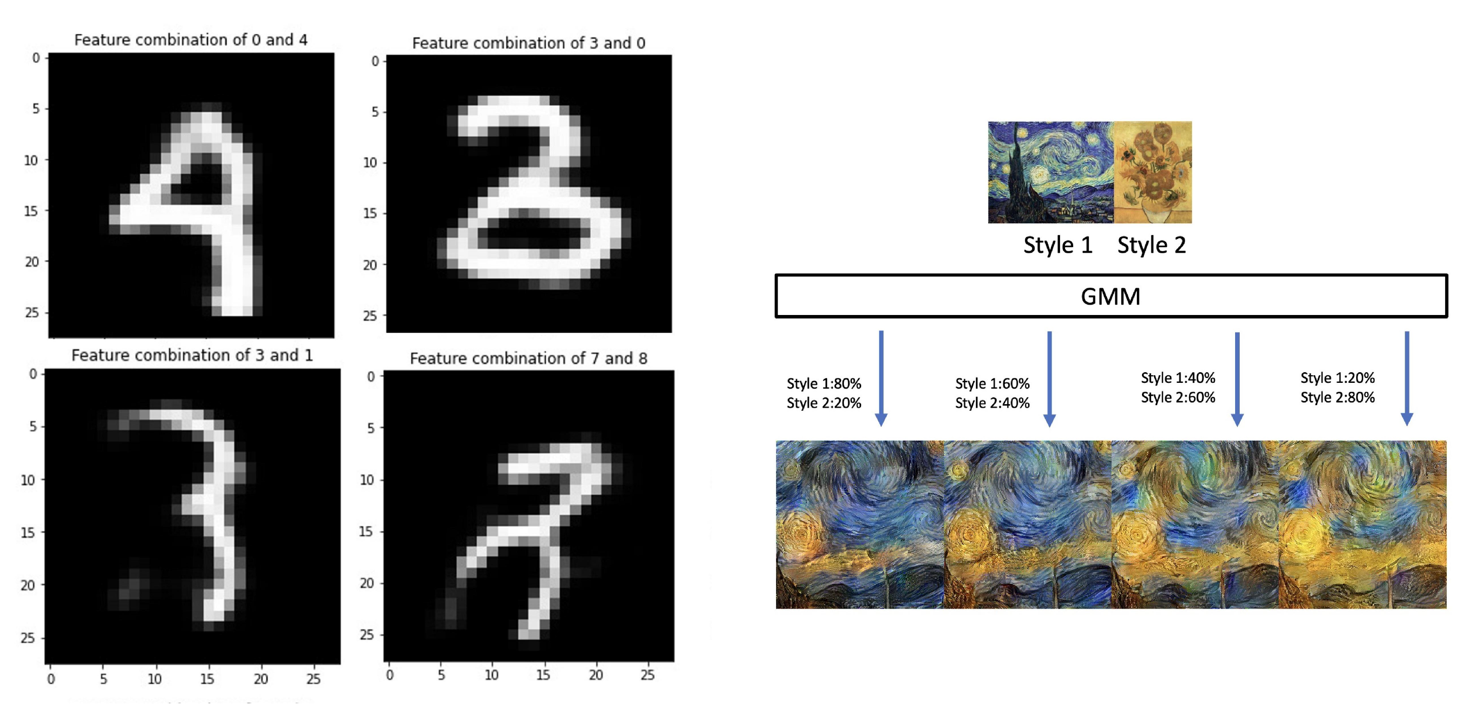
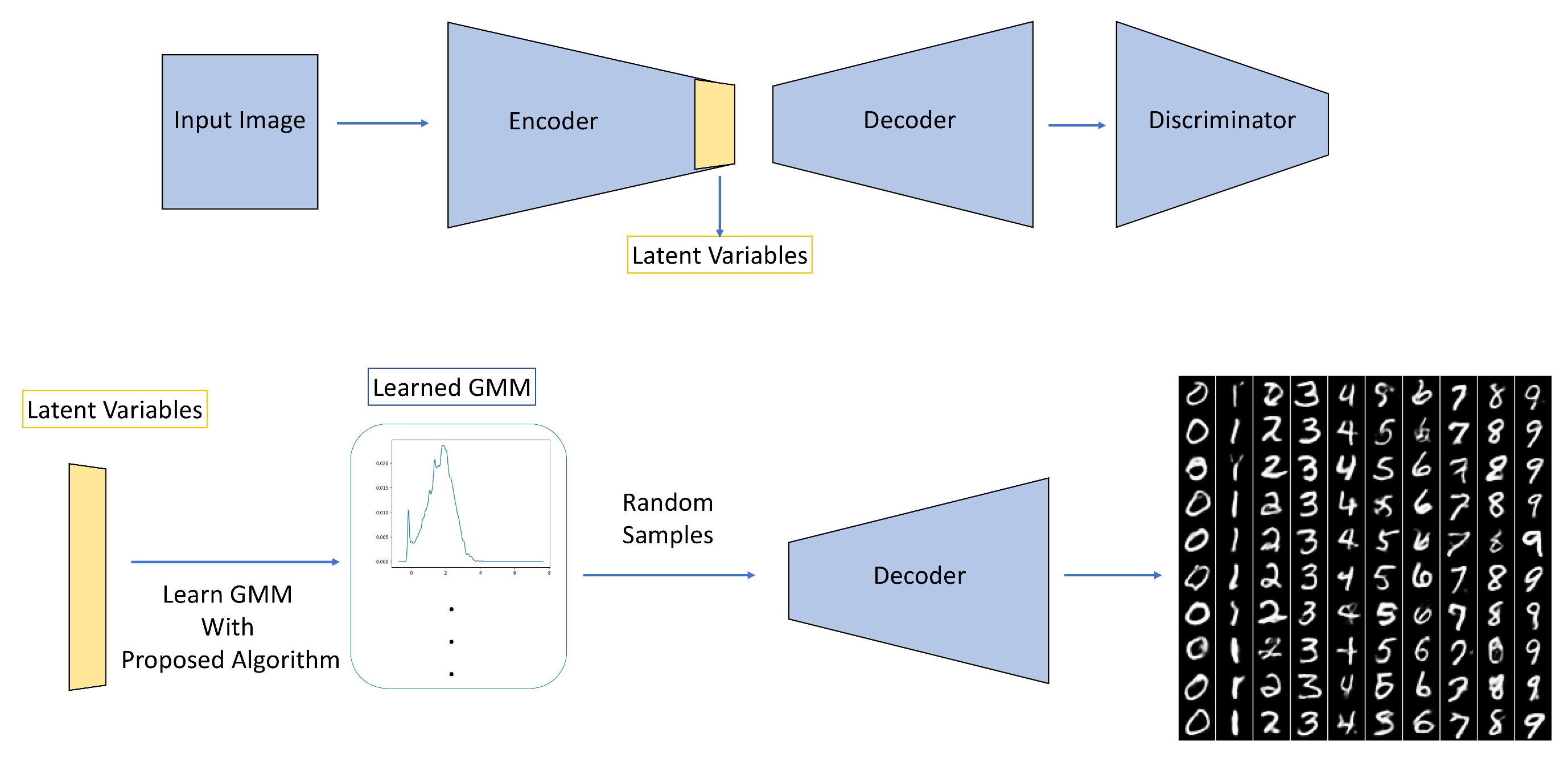
To test whether the proposed method can be beneficial in other neural network applications, we focused on latent variables in neural networks, especially in the generative framework. In this application, the Auto-encoder [8] was tested to demonstrate the effectiveness of the proposed method. In many encoderâdecoder settings, the bottleneck layer is typically responsible for controlling the generated output. The main focus of this application is to consider the latent variables for different classes as random variables, to ensure that we can learn the latent distribution with respect to different classes. Therefore, the latent distributions were treated as GMM and the proposed GMM expansion method was used to learn these distributions. Subsequently, we drew random samples from the learned GMM latent distribution to generate random images for different classes, which were digit 0-9 for the Mnist dataset. The numerical experiment was replicated from a previous study [10]. In an experiment by Kolouri et al. [10], they demonstrated how to employ the Sliced Wasserstein Distance to learn an embedding layer (latent variables) through a GMM. In this application, we learn the latent distributions using the GMM expansion and learning algorithm. The model contains an autoencoder and a straightforward convolutional classification network as the discriminator [24,25,26,27,28]. The entire process is illustrated in Figure 6.

Note that, in our training process, we slightly amended the loss function of GAN. The loss function for this application is expressed by Equation (17).

J^{(G)} = - α \frac{1}{2} E_{z} l o g (1 - D (G (z))) + {‖ x - G (z) ‖}^{2}

(17)

where

J^{(G)}

is the loss of a generator,

α

is a constant to adjust the level of discriminator loss,

\frac{1}{2} E_{z} l o g (1 - D (G (z)))

is the discriminator loss same as [28] and x is the target image and

G (z)

is output image generated by generator. MSE is set as the major source for controlling the direction of learning, and the GAN loss plays a less important role.

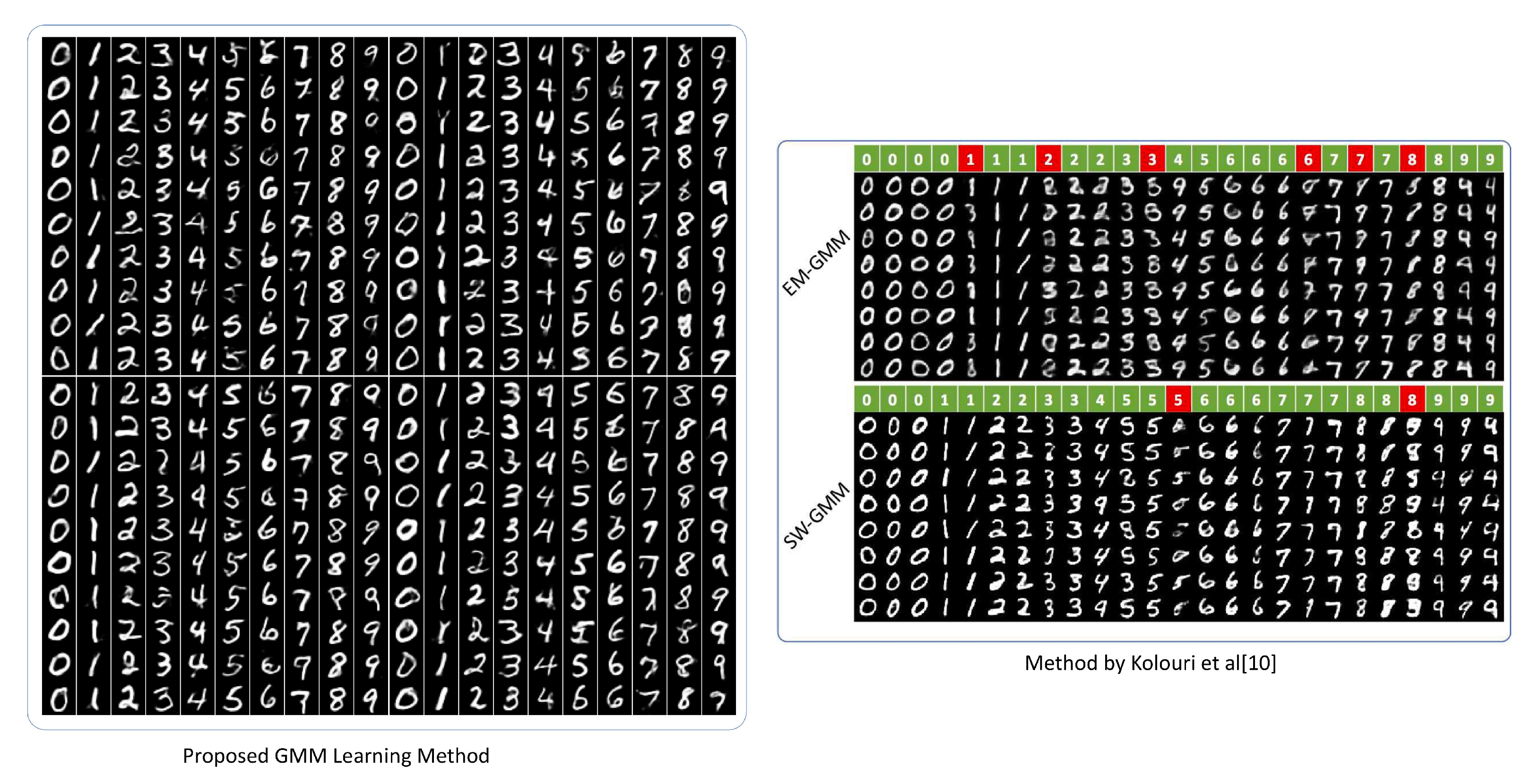
Following up the notation provided in [28], for the generator loss, we multiply

α

to the cross-entropy loss to regulate the discriminator. The addition of Mean Square Loss guides the generator to generate images close to the dataset. When the autoencoder was trained, the values of the latent variables from different classes were gathered, and the proposed method was used to learn the GMMs as latent distributions for each class. After obtaining the latent distributions, the decoder was trained independently with a mean-square error to further match each image. Subsequently, a generator based on the GMM is acquired. Images can be generated by randomly sampling the GMM from different classes. The random samples generated by our model and samples from [10] are shown in Appendix Figure A6. Contrary to the red-highlighted EM-GMM and SW-GMM results, the majority of random samples in our results did not have significant unidentifiable generations, and each class was well separated. The generations across different classes are provided in Appendix Figure A7. Two latent samples are drawn from two different classes and randomly mixed to form a new latent sample for image generation. For instance, the latent in the upper-left subplot is a combination of latent samples from 0 and 4. The output images resembled a 9. These results indicate that the latent distributions learned by the proposed method can separate generations from different classes, and a mixture of latent distributions can retain input category attributes and generate new undefined images.

4.3. Style Transfer

To further demonstrate how latent variables can be transformed into distributional random variables, we modified the style transfer algorithm [9] by converting the Gram matrix into a GMM. The Gram matrix which forms the basis of style transfer, measures the degree of correlation between extracted features as computed by a neural network. A trained VGG19 [29] feature extraction module was applied for feature extraction, as outlined in the original study. When an image is passed through VGG19, it produces output features from each layer. The Gram matrix for the features from each convolutional block was calculated using Equation (18).

G_{i j}^{l} = \sum_{k} F_{i k}^{l} F_{j k}^{l},

(18)

A specific Gram matrix determines the specific algorithmic result. To provide diversity to the algorithm, we can change the learning rate or the weights assigned to style and content features, although performing aggressively can lead to chaotic results. Instead, a distributional Gram matrix can be used, and random sampling of the Gram matrix distributions can produce variations effortlessly. Moreover, similar to application 2, mixing latent across different classes can produce uncategorized images, The random mixture of gram matrix distribution samples from style and content can stochastically create new gram matrix to create variations.

To learn a gram matrix distribution for style and content images, images were randomly cropped and sent to VGG19 independently to obtain sets of feature values. These sets of feature values produce sets of Gram matrices, and the proposed method can be used to learn Gram matrices as GMM distributions. Finally, the same optimization procedure as in the original study [9] was performed using samples from the learned GMM gram matrix distributions. The number of style features in the Gram matrix was determined by the amount of cropped content and style images. For example, we arbitrarily cropped 25 photos from Style 1 and 75 images from Style 2. The sampled Gram matrix will probably comprise

25 %

of the values from style 1 and

75 %

of the values from style 2, as we sample the Gram matrix distributions. Our method is illustrated in Figure 7. Two well-known Vincent Van Gogh works Night" and "Sunflowers" are blended by this algorithm. Appendix Figure A7 shows an increasing number of style mixings in the dataset. This distributional approach changes the fine attributes of the target images but maintains the over style. The output images can be stitched together to create a short video3.

5. Conclusions, Discussion and Future Work

In this study, we present a simple yet effective method called GMM expansion for approximating arbitrary densities. Our method, along with the proposed algorithm, demonstrates competitive performance compared to state-of-the-art techniques such as the Bayesian variational Gaussian mixture method and the EM algorithm. The GMM expansion delivers better accuracy and learning speed. We have found that this method is particularly advantageous for neural networks, as illustrated through three applications. The first application demonstrates that our method is more suitable for modeling distributional outputs in neural network, which helps address non-Gaussian problems. The second and third applications demonstrate how latent variables can be effectively transformed into random variables using the proposed method.

There are several theoretical challenges and areas for further development. We have previously extended this method to high-dimensional densities, which could lead to novel embedding techniques or applications to Gaussian processes. In addition, using GMM to define latent variables as random variables relates to cardinality problems, which involve projecting latent distributions onto data distributions with a neural network. Further exploration of these theoretical problems may contribute to developing advanced generative models, such as incorporating our method into diffusion models [30,31,32].

Appendix A Uniform Distribution Approximation

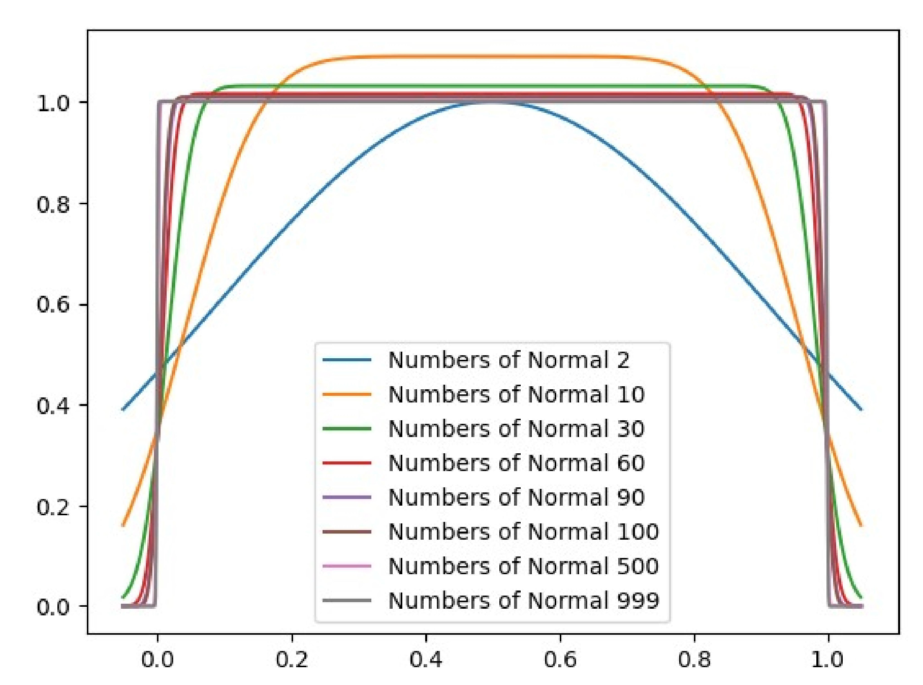
The Gaussian mixture distribution can be approximated by numerical experiments to a uniform distribution under one norm

| | \cdot {| |}_{1}

, so that GMM can be viewed as a step function to ensure prove in Section 2.2. Figure A1 gives the fitting results of different numbers of normal distributions to a uniform distribution. Figure A2 as well as Table A1 demonstrate that the 1-Wasserstein distance between the Gaussian mixture model and uniform distribution is convergent toward zero.

Figure A1. Increase numbers of components in GMM can approximate uniform distribution.

Figure A2. 1-1 wasserstein distance between Gaussian mixture model and Uniform distribution is converge toward zero by increase the size of component distributions.

Consider U and G have bounded support M. For 1-Wasserstein distance, the scheme of transportation

x = G^{- 1} \circ U

leads to

\begin{matrix} W_{1} (g, f) = \int_{M} ∣ G (x) - U (x) ∣ d x, \end{matrix}

(A1)

\begin{matrix} \hat{W_{1} (g, f)} = \sum_{x_{i}} ∣ G (x_{i}) - U (x_{i}) ∣ ▵ x \end{matrix}

(A2)

where

W_{1} (g, f)

and

\hat{W_{1} (g, f)}

are the Wasserstein distance and its approximation, respectively. It is not hard to find, when

W_{1} (g, f) \to 0

, we have

G (x) \approx U (x)

Table A1. W-distance when approximating a uniform distribution using different numbers of Gaussian mixture distributions.

1-Wasserstein Distance of Mixture Gaussian and Uniform Distribution
Numbers of Gaussian	1	2	10	51	101	1001	1997	4997
Wasserstein Distance	0.1838	0.09098	0.01789	0.00463	0.00241	0.00024	0.00012	$4.9 \times 10^{- 5}$

Appendix B Further Analysis and Explanation

This supplement provides further analysis and explanation of the following questions:

1.Does Eq.11 bounded?
2.Why $α$ in Algorithm 1 is this form?
3.Why $σ$ can be treated as hyper-parameter?

To answer these questions, we have to look at the densities on a fine scale. Based on Lemma 1 and Theorem 2, there exists a GMM that approximates a distribution perfectly under the Wasserstein metric space. We can have the following conditions satisfied:

[\begin{matrix} P_{g} \{ω_{0}\} \\ ⋮ \\ P_{g} \{ω_{N}\} \end{matrix}] = [\begin{matrix} P_{f} \{ω_{0}\} \\ ⋮ \\ P_{f} \{ω_{N}\} \end{matrix}],

(A3)

where

P_{g}

is the probability function of GMM and

P_{f}

is the probability function of target distribution. The whole support are split into N small

ω

If the following two conditions are satisfied:

Condition 1: $ω_{i}$ is small enough, the target density is approximately monotone and linear within $ω$
Condition 2: GMM density within $ω$ double crosses the target density.

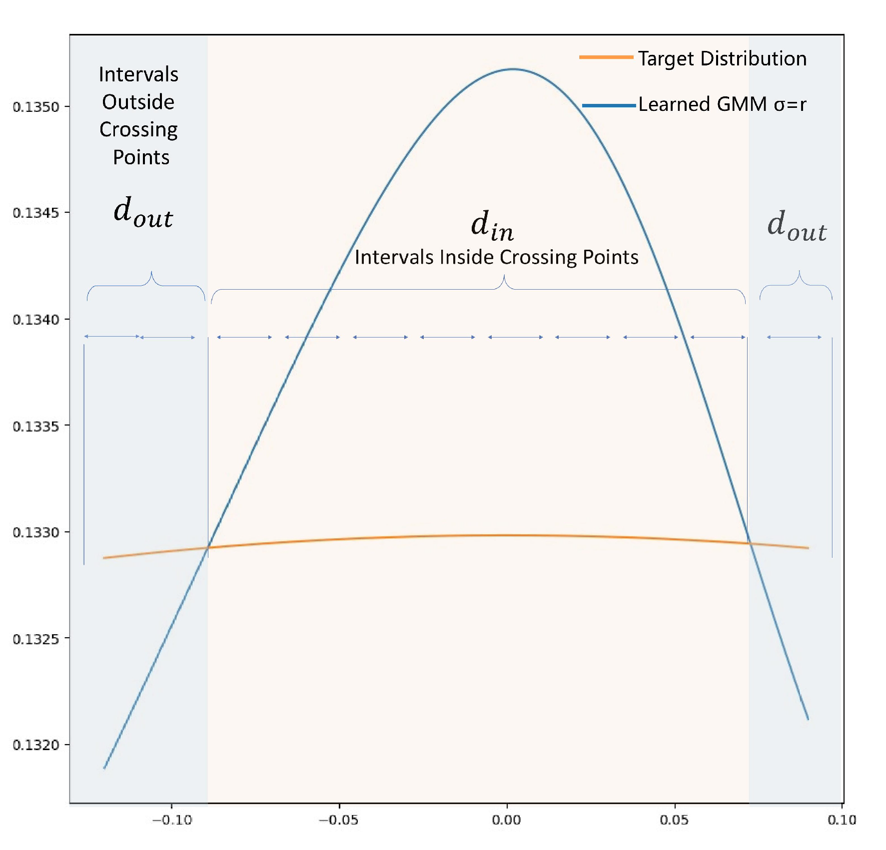
The geometrical structure of GMM and target density within each

ω

is illustrated in Figure A3. The blue line represents the density of GMM, while the orange line represents the density of the target density.

Figure A3. Example of fitted GMM and target density in region

ω_{i}

Figure A3. Example of fitted GMM and target density in region

ω_{i}

To further split

ω_{i}

evenly into smaller areas, each area should have a length of d. Given the condition that the GMM density double crosses the target density,

g (x) \geq f (x)

, for all regions lying between the cross points so that:

\begin{matrix} P_{g} \{d_{i n}\} \geq P_{f} \{d_{i n}\}, \end{matrix}

where

d_{i n}

represent any region lie between cross points.

On the contrary,

g (x) \leq f (x)

, for all regions lying outside of cross points so that:

\begin{matrix} P_{g} \{d_{o u t}\} \leq P_{f} \{d_{o u t}\}, \end{matrix}

where

d_{o u t}

represents any region lying between cross points.

Recall that in Section 2.3, Equation (11),

L (ω_{i}) = \frac{1}{2} \sum_{j = 1}^{m} | P_{f} \{d_{i j}\} - P_{g} \{d_{i j}\} | .

(A4)

We can conclude that

L (ω_{i})

is bounded because for any interval

d_{i j}

∣ P_{f} \{d_{i j}\} - P_{g} \{d_{i j}\} ∣ \leq MAX (P_{g} (d_{i n})) - MIN (P_{g} (d_{o u t})) < τ,

(A5)

This led to the reasoning behind

α

. It is designed by choosing a value of

Max (P_{g} (d_{i n})) - MIN (P_{g} (d_{o u t}))

. In practice, we applied

β (P \{μ_{i} \pm \frac{d}{2}\} - P \{μ_{i} + \frac{r}{2} - d < x \leq μ_{i} + \frac{r}{2})\}

(A6)

β (P \{μ_{i} \pm \frac{d}{2}\} - P (μ_{i} - \frac{r}{2} \leq x \leq μ_{i} - \frac{r}{2} + d))

(A7)

where P is the probability of a Gaussian distribution. The parameter

β

can be seen as the learning rate or as a factor that scales P into

P_{g}

. Generally, in practice, we choose

0.01 \leq β \leq 1

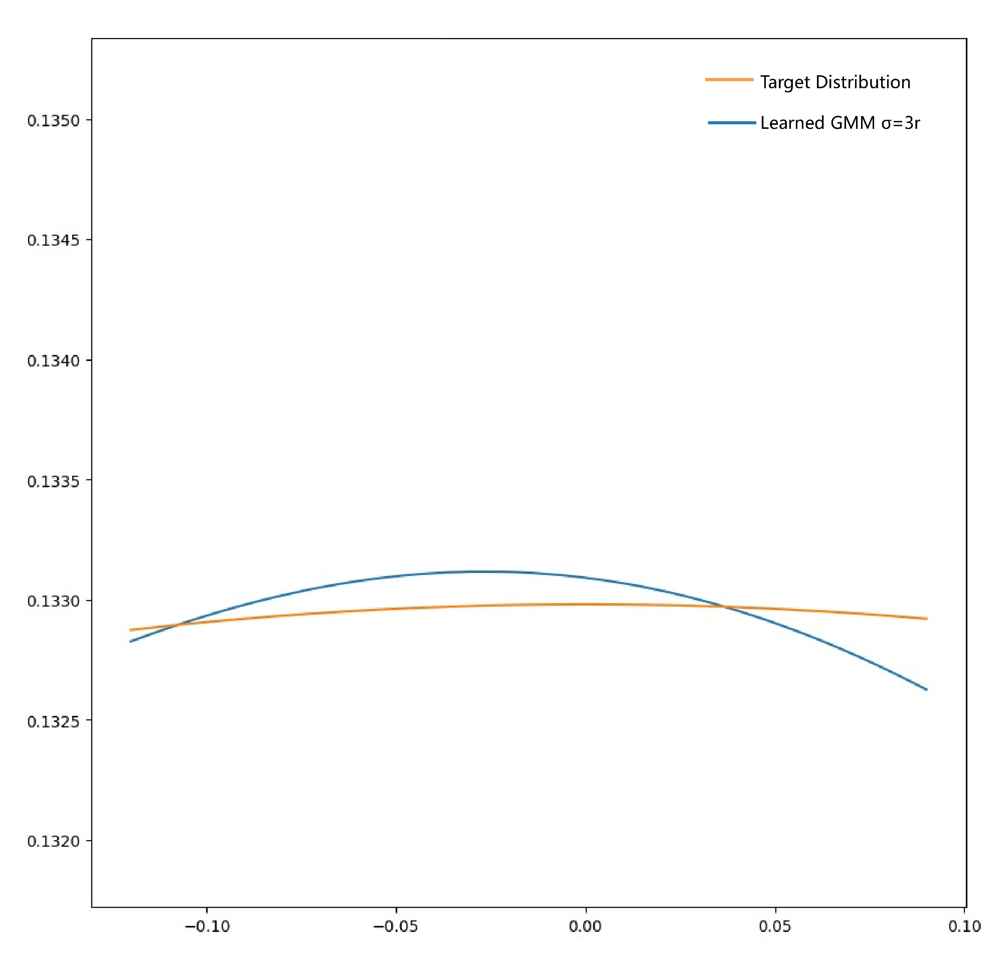
Figure A4. Example of GMM and target density in region

ω_{i}

with larger

σ

Figure A4. Example of GMM and target density in region

ω_{i}

with larger

σ

Finally, these illustrations also reveal the reasoning behind why

σ

is a hyperparameter. The GMM in Figure A3 uses

σ = 1 * r

. If

σ

is tuned to a larger value, it leads to the result shown in Figure A4, where

σ = 3 * r

. The

σ

of each Gaussian component becomes a universal smoothness parameter that controls the kurtosis of each normal component. A larger

σ

produces an overall smoother density.

Appendix C Additional Experiment Results

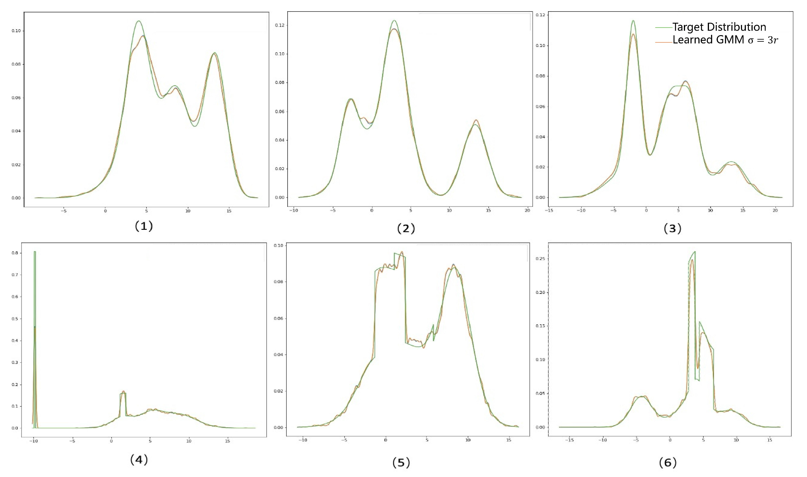
Figure A5. Other trained examples.

Figure A6. Result comparison.

Figure A7. Feature Mixture with GMM

In this appendix, we give more results from the related experiments in Section 3 and 4. Figure A5 shows the fitting of more different types of distributions using the proposed method. Figure A6 is a comparison with the results of Kolouri et al. [10]. Figure A7 is a detailed presentation of Figure 6 and Figure 7.

1	https://scikit-learn.org/
2	https://tensorflow.google.cn/probability
3	https://youtu.be/yP22_ycAqMA

References

G. J. McLachlan and S. Rathnayake, “On the number of components in a gaussian mixture model,” Wiley Interdisciplinary Reviews: Data Mining and Knowledge Discovery, vol. 4, no. 5, pp. 341–355, 2014.
J. Li and A. Barron, “Mixture density estimation,” Advances in neural information processing systems, vol. 12, 1999.
C. R. Genovese and L. Wasserman, “Rates of convergence for the gaussian mixture sieve,” The Annals of Statistics, vol. 28, no. 4, pp. 1105–1127, 2000.
C. Blundell, J. Cornebise, K. Kavukcuoglu, and D. Wierstra, “Weight uncertainty in neural network,” in International Conference on Machine Learning. PMLR, 2015, pp. 1613–1622.
Y. Gal, “What my deep model doesnât know,” Personal blog post, 2015.
A. Kendall and Y. Gal, “What uncertainties do we need in bayesian deep learning for computer vision?” Advances in neural information processing systems, vol. 30, 2017.
A. Der Kiureghian and O. Ditlevsen, “Aleatory or epistemic? does it matter?” Structural safety, vol. 31, no. 2, pp. 105–112, 2009.
D. P. Kingma and M. Welling, “Auto-encoding variational bayes in 2nd international conference on learning representations,” in ICLR 2014-Conference Track Proceedings, 2014.
L. A. Gatys, A. S. Ecker, and M. Bethge, “A neural algorithm of artistic style,” arXiv preprint arXiv:1508.06576, 2015.
S. Kolouri, G. K. Rohde, and H. Hoffmann, “Sliced wasserstein distance for learning gaussian mixture models,” in Proceedings of the IEEE Conference on Computer Vision and Pattern Recognition, 2018, pp. 3427–3436.
A. P. Dempster, N. M. Laird, and D. B. Rubin, “Maximum likelihood from incomplete data via the em algorithm,” Journal of the Royal Statistical Society: Series B (Methodological), vol. 39, no. 1, pp. 1–22, 1977.
J. Du, Y. Hu, and H. Jiang, “Boosted mixture learning of gaussian mixture hidden markov models based on maximum likelihood for speech recognition,” IEEE transactions on audio, speech, and language processing, vol. 19, no. 7, pp. 2091–2100, 2011.
J. J. Verbeek, N. Vlassis, and B. Kröse, “Efficient greedy learning of gaussian mixture models,” Neural computation, vol. 15, no. 2, pp. 469–485, 2003.
C. Jin, Y. Zhang, S. Balakrishnan, M. J. Wainwright, and M. I. Jordan, “Local maxima in the likelihood of gaussian mixture models: Structural results and algorithmic consequences,” Advances in neural information processing systems, vol. 29, 2016.
C. Améndola, M. Drton, and B. Sturmfels, “Maximum likelihood estimates for gaussian mixtures are transcendental,” in International Conference on Mathematical Aspects of Computer and Information Sciences. Springer, 2015, pp. 579–590.
N. Srebro, “Are there local maxima in the infinite-sample likelihood of gaussian mixture estimation?” in International Conference on Computational Learning Theory. Springer, 2007, pp. 628–629.
Y. Chen, T. T. Georgiou, and A. Tannenbaum, “Optimal transport for gaussian mixture models,” IEEE Access, vol. 7, pp. 6269–6278, 2018.
P. Li, Q. Wang, and L. Zhang, “A novel earth mover’s distance methodology for image matching with gaussian mixture models,” in Proceedings of the IEEE International Conference on Computer Vision, 2013, pp. 1689–1696.
C. Beecks, A. M. Ivanescu, S. Kirchhoff, and T. Seidl, “Modeling image similarity by gaussian mixture models and the signature quadratic form distance,” in 2011 International Conference on Computer Vision. IEEE, 2011, pp. 1754–1761.
B. Jian and B. C. Vemuri, “Robust point set registration using gaussian mixture models,” IEEE transactions on pattern analysis and machine intelligence, vol. 33, no. 8, pp. 1633–1645, 2010.
G. Yu, G. Sapiro, and S. Mallat, “Solving inverse problems with piecewise linear estimators: From gaussian mixture models to structured sparsity,” IEEE Transactions on Image Processing, vol. 21, no. 5, pp. 2481–2499, 2011.
W. M. Campbell, D. E. Sturim, and D. A. Reynolds, “Support vector machines using gmm supervectors for speaker verification,” IEEE signal processing letters, vol. 13, no. 5, pp. 308–311, 2006.
K. P. Murphy, “Machine learning: A probabilistic perspective (adaptive computation and machine learning series),” pp. 344–345, 2018.
H. Schwenk and Y. Bengio, “Training methods for adaptive boosting of neural networks,” Advances in neural information processing systems, vol. 10, 1997.
G. E. Hinton and R. Zemel, “Autoencoders, minimum description length and helmholtz free energy,” Advances in neural information processing systems, vol. 6, 1993.
Y. LeCun, “The mnist database of handwritten digits,” http://yann.lecun.com/exdb/mnist/, 1998.
J. Li, W. Monroe, T. Shi, S. Jean, A. Ritter, and D. Jurafsky, “Adversarial learning for neural dialogue generation,” arXiv preprint arXiv:1701.06547, 2017.
I. Goodfellow, “Nips 2016 tutorial: Generative adversarial networks,” arXiv preprint arXiv:1701.00160, 2016.
K. Simonyan and A. Zisserman, “Very deep convolutional networks for large-scale image recognition,” arXiv preprint arXiv:1409.1556, 2014.
J. Ho, A. Jain, and P. Abbeel, “Denoising diffusion probabilistic models,” Advances in Neural Information Processing Systems, vol. 33, pp. 6840–6851, 2020.
Y. Song and S. Ermon, “Generative modeling by estimating gradients of the data distribution,” Advances in Neural Information Processing Systems, vol. 32, 2019.
J. Sohl-Dickstein, E. Weiss, N. Maheswaranathan, and S. Ganguli, “Deep unsupervised learning using nonequilibrium thermodynamics,” in International Conference on Machine Learning. PMLR, 2015, pp. 2256–2265.
DM. Blei, A. Kucukelbir, and JD. McAuliffe, “Variational inference: A review for statisticians,” in Journal of the American statistical Association. 2017, 112(518), pp.859–877.
C. Villani, “Optimal transport: old and new,” in Berlin: springer. 2009, 112(518), pp.93–113.
CM. Bishop, NM. Nasrabadi, “Pattern recognition and machine learning,” in New York: springer. 2006, pp.423–517.
S. Balakrishnan, MJ. Wainwright, B. Yu, “Statistical guarantees for the EM algorithm: From population to sample-based analysis.,” in Ann. Statist. 2017, 45 (1) 77 - 120. [CrossRef]
H. Attias, “A variational baysian framework for graphical models,” in Advances in neural information processing systems, 12.. 1999.

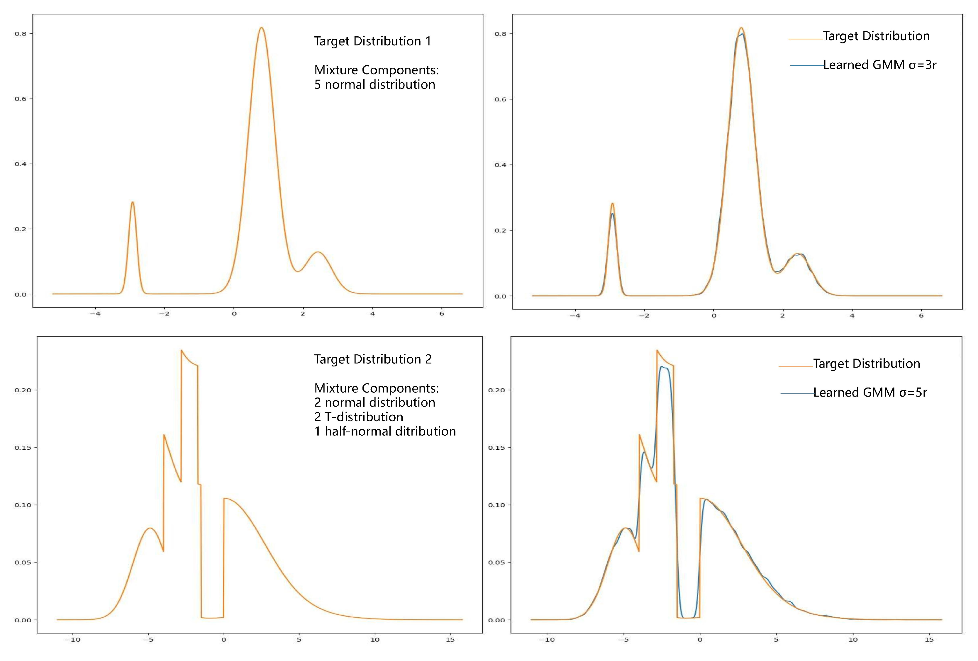
Figure 1. Learning smooth and non-smooth densities using GMM expansion and proposed algoirthm. Target density of upper plot is a mixture of continuous, smooth densities. Plots on the left shows how target densities are built and plots on the right shows the comparison of target densities and learned GMM.

Figure 2. Learning Process of Proposed Algorithm

Figure 3. Proposed Algorithm for 2 dimensional distribution

Figure 5. Neural Network Application 1. GMM expansion improve neural network performance in probabilistic prediction.

Figure 6. Neural Network Application 2. Learn latent distribution of autoencoder using proposed GMM expansion method.

Figure 7. Neural Network Application 3. Learn gram matrices distributions using proposed GMM expansion method.

Table 1. Average TVD of 20 Experiments With 8 random Gaussian Components. Data size: 5000 data points.

Average TVD For Smooth Densities
$σ = 1 * r$	$σ = 2 * r$	$σ = 3 * r$
$L =$ 0.035495	$L =$ 0.025455	$L =$ 0.022248

Table 2. Average TVD of 20 Experiments With 8 random Components which consist of Normal, T and Uniform distribution. Data size: 5000 data points.

Average TVD For Non-Smooth Densities
$σ = 1 * r$	$σ = 2 * r$	$σ = 3 * r$
$L =$ 0.04456	$L =$ 0.04369	$L =$ 0.04716

Table 3. Average TVD of 25 Experiments With different numbers of components compares with data size 20000 data points and 50000 data points.

Average TVD of 30 Experiments with Data size 20000
Numbers of Components
10	30	50	100	200	500	1000
$L = 0.355$	$L = 0.168$	$L = 0.100$	$L = 0.0389$	$L = 0.0148$	$L = 0.0163$	$L = 0.0189$
Average TVD of 30 Experiments with Data size 50000
Numbers of Components
10	30	50	100	200	500	1000
$L = 0.356$	$L = 0.182$	$L = 0.105$	$L = 0.033$	$L = 0.013$	$L = 0.0102$	$L = 0.0145$

Table 4. Mean and standard deviation of TVD and training time. Each target distribution is sampled 2000 data points for learning.

Average TVD of 50 Experiments
Numbers of Components
	20	100	200	500	1000
Proposed Method	$0.193 \pm 0.060$	$0.066 \pm 0.0164$	$0.058 \pm 0.007$	$0.077 \pm 0.006$	$0.105 \pm 0.006$
EM K-mean	$0.076 \pm 0.0085$	$0.143 \pm 0.006$	$0.215 \pm 0.009$	$0.352 \pm 0.019$	$0.437 \pm 0.050$
EM Random	$0.076 \pm 0.011$	$0.134 \pm 0.008$	$0.192 \pm 0.010$	$0.295 \pm 0.022$	$0.373 \pm 0.036$
BVI	$0.090 \pm 0.025$	$0.096 \pm 0.030$	$0.098 \pm 0.029$	$0.096 \pm 0.028$	$0.103 \pm 0.031$
Average Training Time of 50 Experiments
	20	100	200	500	1000
Proposed Method	$0.0004 \pm 5.4 \times 10^{- 5}$	$0.0012 \pm 0.0002$	$0.0021 \pm 0.0005$	$0.0038 \pm 0.0003$	$0.008 \pm 0.001$
EM K-mean	$0.182 \pm 0.0964$	$0.482 \pm 0.073$	$0.952 \pm 0.090$	$2.354 \pm 0.494$	$2.340 \pm 0.667$
EM Random	$0.175 \pm 0.0213$	$0.555 \pm 0.0462$	$1.096 \pm 0.162$	$2.710 \pm 0.534$	$4.548 \pm 1.428$
BVI	$1.610 \pm 0.212$	$6.265 \pm 0.251$	$12.234 \pm 0.166$	$25.505 \pm 0.358$	$46.931 \pm 1.416$

Disclaimer/Publisher’s Note: The statements, opinions and data contained in all publications are solely those of the individual author(s) and contributor(s) and not of MDPI and/or the editor(s). MDPI and/or the editor(s) disclaim responsibility for any injury to people or property resulting from any ideas, methods, instructions or products referred to in the content.

© 2024 by the authors. Licensee MDPI, Basel, Switzerland. This article is an open access article distributed under the terms and conditions of the Creative Commons Attribution (CC BY) license (http://creativecommons.org/licenses/by/4.0/).

Copyright: This open access article is published under a Creative Commons CC BY 4.0 license, which permit the free download, distribution, and reuse, provided that the author and preprint are cited in any reuse.

MDPI Initiatives

Important Links

Choose an area of interest and we will send you notifications of new preprints at your preferred frequency.

Disclaimer

An Efficient Gaussian Mixture Model and Its Application to Neural Network

Abstract

1. Introduction

2. GMM Expansion

2.1. The Concept of GMM Expansion

2.2. Approximate Arbitrary Density by GMM Expansion

2.3. Total Variation Distance Analysis For Small Region

2.4. Learning Algorithm and Convergence

3. Numerical Experiments

3.1. Density Approximation

3.2. Comparison Study

4. Neural Network Application

4.1. Probabilistic Output

4.2. Mnist Data Set of Handwritten Digits Generation

4.3. Style Transfer

5. Conclusions, Discussion and Future Work

Appendix A Uniform Distribution Approximation

Appendix B Further Analysis and Explanation

Appendix C Additional Experiment Results

References

MDPI Initiatives

Important Links

Subscribe