1. Introduction
Deepfakes are manipulated images or videos that usually are an attempt to affect the image or reputation of an individual, or deepfakes are used to spread disinformation. There are times when the creation of deepfakes is for good-faith intentions, such as when MIT created a deepfake video of a speech by President Nixon alleging a failed Apollo-11 mission [
1], or when American director Jordan Peele impersonated President Obama [
2] to present a speech that seemed out of character. The altered, hyper-realistic images and videos are enough to convince people of their legitimacy. Nicolas Cage appears in a collection of videos [
3] where the actor appears in movies that he was never cast in. Deepfake creation stems from machine learning methods [
4] that have been improved upon to now using advanced deep learning techniques involving convolutional neural networks (CNN) [
5], which are deep learning models that consist of convolutional layers. These layers are able to learn patterns, or features, in images based on sub-groupings of pixels within a larger image. These feature detectors are called filters, or kernels, and are "activated" when the layer receives input from an image containing similar pixel structures. This essentially is a form of learning the contents of images, and these filters can be used with other images to detect if they contain similar pixel patterns. Since these filters are learned by the deep learning model, these models then have the ability to recreate images that would activate the filters, thus creating a deepfake [
5,
6,
7].
In recent years, there has been an increase in image and video data that only shows the periocular region instead of the entire face. This is largely due to the increase in people wearing masks because of the COVID-19 pandemic. The less-revealing faces already inhibit facial inter-personal facial recognition, but this lowered recognition also makes it easier for a deepfake to pass as realistic to a human observer. Deepfake creators that rely on face swapping and mimicry focus on prominent facial features to manipulate, such as the eyes, nose, and mouth [
5]. These features along with their expected, artifact-free observation, allow people to discern a manipulated image yet when most of the face is covered or hidden, people have less information in front of them to make that decision. Although deepfake periocular image data can be created, the process to create them still is believed to generate artifacts and inconsistencies within the created images that can be detected not only by human eyes, but also with deep learning models.
Deep learning methods have been used before to detect deepfakes, such as CNN and long short-term memory (LSTM) but there has been a lack of combining various computer vision algorithms with deep learning models. Deep learning models alone tend to perform well, that including other feature extraction methods can incur unneeded overhead without increasing performance. For example, feature extraction using scale-invariant feature transform takes a long time to extract a smaller set of features than compared to histogram of oriented gradients. Both computer vision methods can be used for object and edge detection, although the quality of the extracted features may differ significantly.
Compared to CNN, many of these computer vision methods are able to perform feature extraction at a much faster rate while using fewer resources, although classification performance is poorer. This research intends to combine feature extraction and CNN for deepfake detection, and to compare the performance of these combined models. As of this paper, there have not been significant strides made in the deep learning field for periocular-based deepfake detection. This paper will show that deep learning models using different computer vision feature extraction methods, along with combining these various models, can detect deepfakes at a significantly higher accuracy focusing only on the periocular region. Models designed around smaller smaller amounts of information are useful when only these smaller pools of data are available.
A simple example of a CNN is a model that can distinguish pictures containing cats from pictures containing dogs, or even being able to count the number of cats and dogs in a picture, along with their breed. More robust CNN are able to generate new images containing a cat or dog, to further the example. Common methods of deepfake generation involve cutting and pasting [
5], or called swapping [
8,
9,
10], the face of one person onto another. This swapping leaves artifacts in the produced image that may be noticeable to the human eye but smaller details can be detected by a machine [
9,
11]. In order to increase realism in the manipulated images, smoothing and brushing techniques are used along the bounding box of the swapped face, with key facial landmarks mapped to match the movement of the actor on the original image. The bounding box has been a focus of research [
5,
8] in detecting deepfakes since using a mask to swap a face naturally creates edges, making edge detection possible [
12]. Alterations within the swapped face are less likely to produce consistent edges since their creation is based on image augmentation [
13], as opposed to image masking.
In this paper, the dataset DeepFakeDetection [
14,
15] is used for performance evaluation. These models may then be used on other datasets from the FaceForensics++ [
14] collection to compare their results for a more general evaluation. DeepFakeDetection consists of one thousand unaltered videos, and three thousand manipulated videos based on the original videos. Since the source is video data, and frames will need to be extracted to have image data, a substantially large portion of the dataset would look similar, in that each frame of a video is only slightly different from the neighboring frame in most cases, in some cases, the neighboring frame is the exact same.
The use of CNNs for image, or image-like, learning is widely employed since the convolutional process creates smaller, stacked regions of learnable features while preserving input data. This process is performed within layers called . Between convolutions, the feature map, or activation map, will become more dense, or deeper, while the two-dimensional nature of the image data at most remains the same, while in many cases, decreases as the number of filters increase across layers. These filters activate when a learned feature is passed through them. This means that we can have many trainable filters, trained on smaller, deeper dimensions of image data to detect features that would indicate if an image is original, unaltered media, or if it has been altered and could be a deepfake.
Along with using convolutional layers, we explore some other methods that can be used to extract features from image data for deepfake classification. These methods are Scale-Invariant Feature Transform [
11,
16] (SIFT) and Histogram of Oriented Gradients [
17] (HOG). SIFT features are useful in that the features, when clustered together, are used to represent objects and biological markers within an image. These objects and markers are able to be mapped across various images, regardless of changes in scale or orientation. This presents a useful tool for object detection that can be used to detect distinguishing features in deepfake images. HOG features, when seen as in image, is more akin to edge detection and contour detection. HOG features represent changes in angle gradients, or slopes, and contrast across pixel data using Gaussian derivatives. When the image data is viewed, it is shown as a collection of angled vectors that outline the various objects in the image.
Ensemble models offer a relatively simple way to include multiple different features as input for the same process. Typically, deep neural networks have a single set of features, or a batch of similar features, for learning. These more complex models allow a single input, such as an image, to be represented by different types of features. In the case of this article, the different type of features are convolutional features, SIFT features, and HOG features. Since these features are extracted using different processes, one set of features may contain unique data that can be used effectively to distinguish original media from deepfakes. In this article, we describe how an ensemble model can be used with various feature extraction tools to accurately detect deepfakes with high performance. We will also explain the construction of the model and their performance on different datasets.
2. Proposed Methods
This section will discuss the methods used to build a CNN model for feature extraction and classification, and also the use of machine learning algorithms for feature extraction. This section will also include the performance of the models along with a comparison of their metrics.
2.1. Dataset
The primary dataset comes from the
++ [
14] collection of deepfakes. The current collection consists of six sets of deepfakes ccreated using different methods of deepfake creation. A few of the datasets within
++ are
,
,
, and
. The DeepFakeDetection [
14,
15], created by Google and Jigsaw, is used as the experimental dataset. This dataset consists of 1000 original, unaltered videos containing twenty-eight actors. There are also 3000 manipulated videos, called deepfakes. The deepfakes are produced from the original videos using face swapping methods. To balance original and manipulated videos, every third manipulated video per actor is used for every original video per actor. The videos from the datasets are also labeled as either "real" or "fake," along with the extracted frames from each video being labeled based on their respective source. For example, frames extracted from the video named "fake_000.mp4" will have the name "fake_xxxx.jpg," where "xxxx" is an incremental number based on the number of total extracted frames, and the beginning of the file name, such as "fake" corresponds to the frame’s label. Since the proposed model is a binary classifier, there are only two target labels for prediction: real and fake. Real would suggest the image is unaltered, unmanipulated, while fake would suggest the image is a deepfake.
2.2. Dataset Frame Extraction
Using the
[
18] library
[
19], videos are loaded and frames saved. Since image data is coming from videos, the majority of frames tend to be nearly identical to the previous and successive frame. Having a large amount of similar images where the key features may not change within each frame can lead to the dataset having increased homogeneity. To mitigate this, a frame is saved every
, and 100 frames are saved per loaded video. After extracting all of the necessary frames, there is a total of
images
2.3. Periocular Region Extraction
Face detection and facial landmark localizing was done using the trained deep neural network Multitask Cascaded Neural Network (MTCNN) [
20]. By using a trained neural network, we can retain detected faces with a confidence of
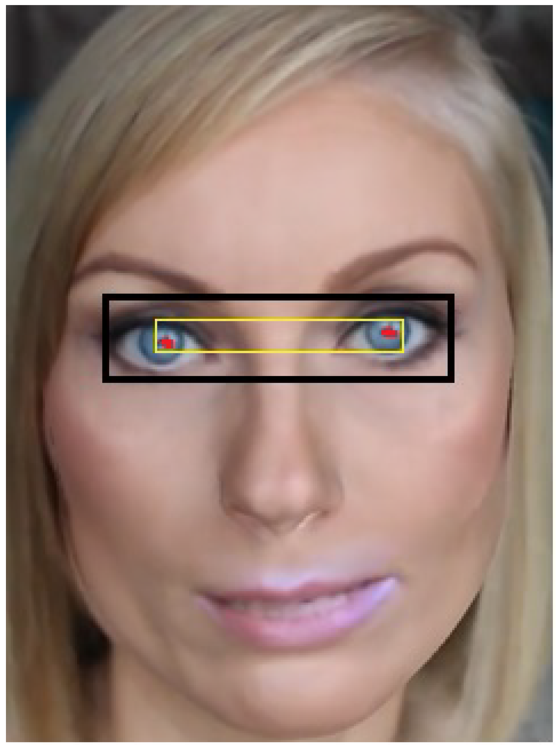
, and ignore faces with lower confidence. MTCNN also provides the location of detected facial landmarks, such as the left eye, right eye, nose, and mouth corners. Using the locations of the eyes, we create a bounding box with extra padded space to include the areas surrounding the eyes, such as the eyebrows, and top of the nose region. An example of this process can be seen in
Figure 1. The returned face by MTCNN is not truly a face, but a dictionary. This dictionary contains the keys
,
, and
. The value of
is a dictionary containing coordinates for facial landmark locations
,
,
,
, and
, where
is the bounding box around the detected face,
is the confidence of the model in the detected face,
is the eye on the left side from the perspective of the viewer,
is the corner of the mouth on the left side from the perspective of the viewer, and
is the tip of the nose. To prevent having two separate eyes to manage, the pixel locations of the bottom right- and top rightmost pixels can be used with the bottom left- and top leftmost pixels to create a single bounding box containing both eyes. This bounded box is then padded with extra pixels since the landmark locations provided by MTCNN are centered on the eyes. This box is then used to crop the eye region from the face image and save the eye region as an image. The images are then resized to height and width
. After extraction, the image database consists of
color images of shape
, where exactly half,
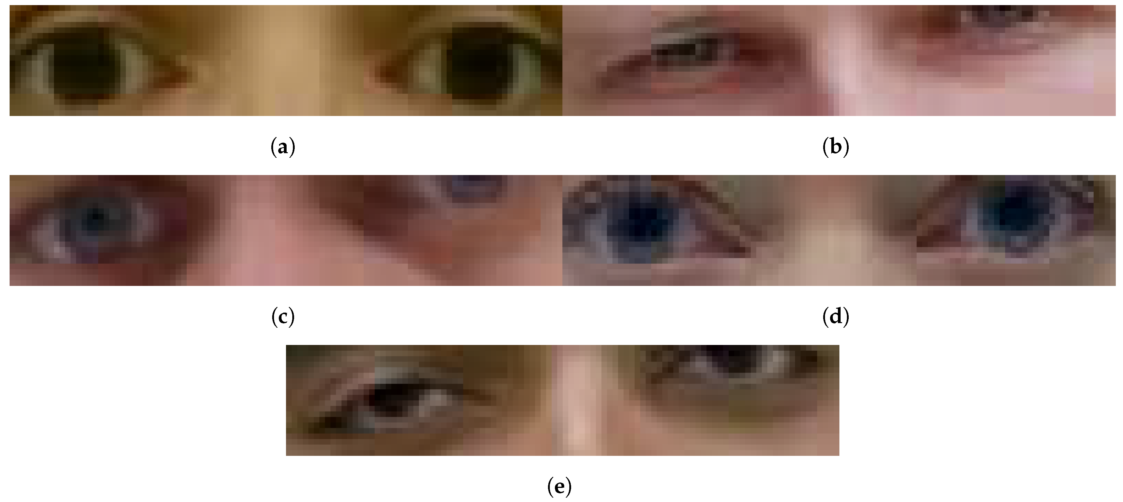
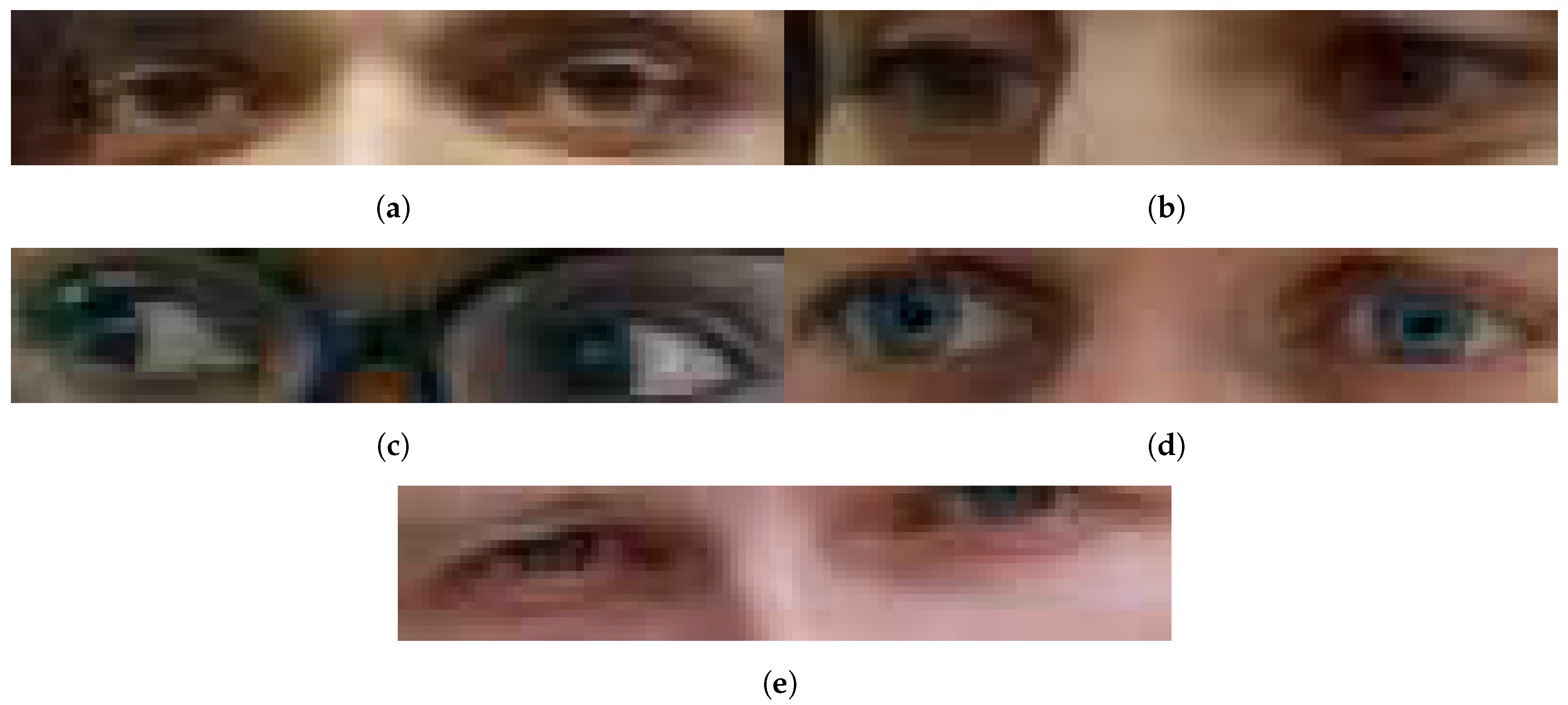
, come from original, unaltered videos, and the other half come from the deepfake videos. Sample input images for the model after frame extraction are shown in
Figure 2 and
Figure 3.
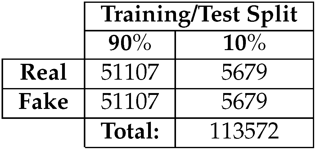
Before using the data with a model, the input dataset must be split into training and testing sets. The dataset will be split with a ratio of
to match
Table 1, where exactly half of the dataset belongs to the
class and the other half belongs to the
class:
2.4. Convolutional Neural Network Model
Convolutional neural networks (CNN) use
to create feature maps of images. These feature maps consist of filters that activate when they "see" a similarly learned feature from the training data in images, such as edges or color, or a pattern. CNN have been a popular choice for object recognition in images and deepfake detection [
8,
10,
21,
22,
23] because of their ability to learn features in images and create high dimensionality generalizations from images without sacrificing information from the input images. As images are passed through convolutional layers, a kernel of a fixed size, typically
,
, or other sizes, the kernel learns features about pixels and their surrounding data points, which would be other pixels, thus preserving the relationship between pixels [
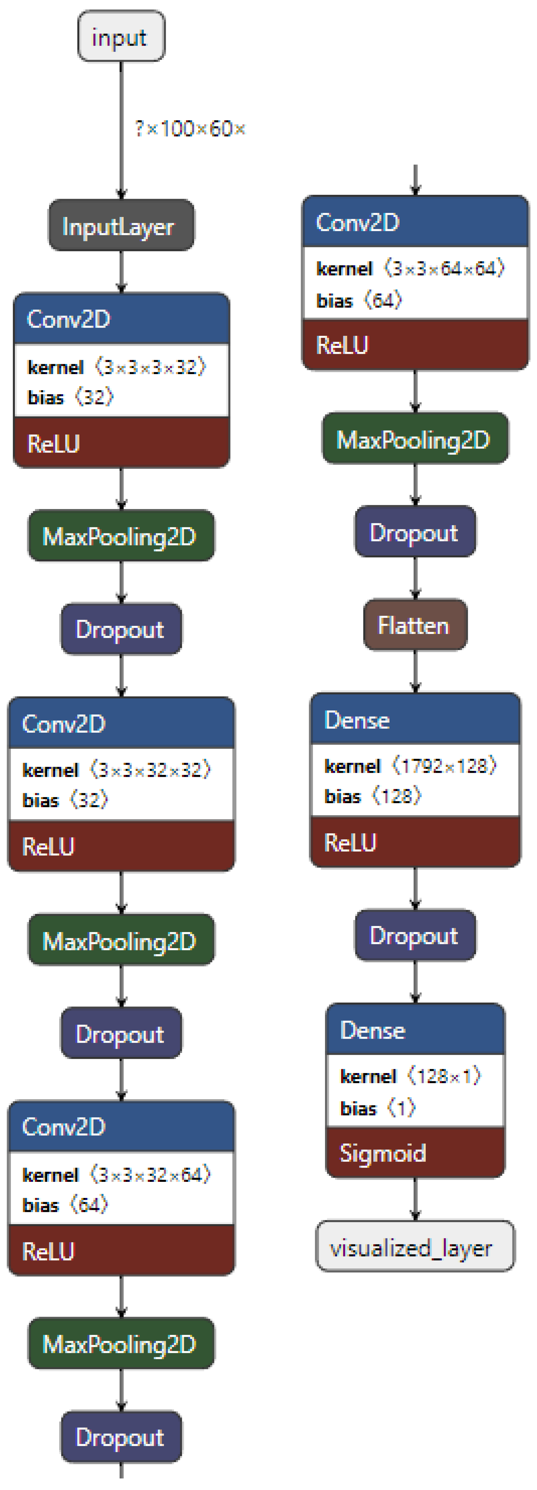
24]. Building a CNN requires building upon convolutional layers. We design a CNN model containing four convolutional "blocks," where each block contains a
, a
, and a
. The first two convolutional layers have 32 filters, and the last two have 64 filters. All convolutional layers use the
(ReLU) activation function and a stride of 3. ReLU improves the generalization ability of convolutional layers with an effect similar to Batch Normalization [
25]. Using a dropout of
provided enough random, turned-off neurons to reduce overfitting. Finally, two
layers are used, with the first having 128 neurons and relu activation function, and the second, classifying layer having one neuron and the
activation function. Since the labels refer to the classes, and there are only two possible classes for this binary classification problem, we use the
loss function. The equation for calculating the loss function is shown in Equation (
1), where
y is the binary class value, either 0 or 1, and
p is the predicted probability that the predicted element belongs to class 1. The optimizer
is used with the learning rate set to
.
Figure 4 shows the architecture of the standalone CNN model used for feature extraction and classification.
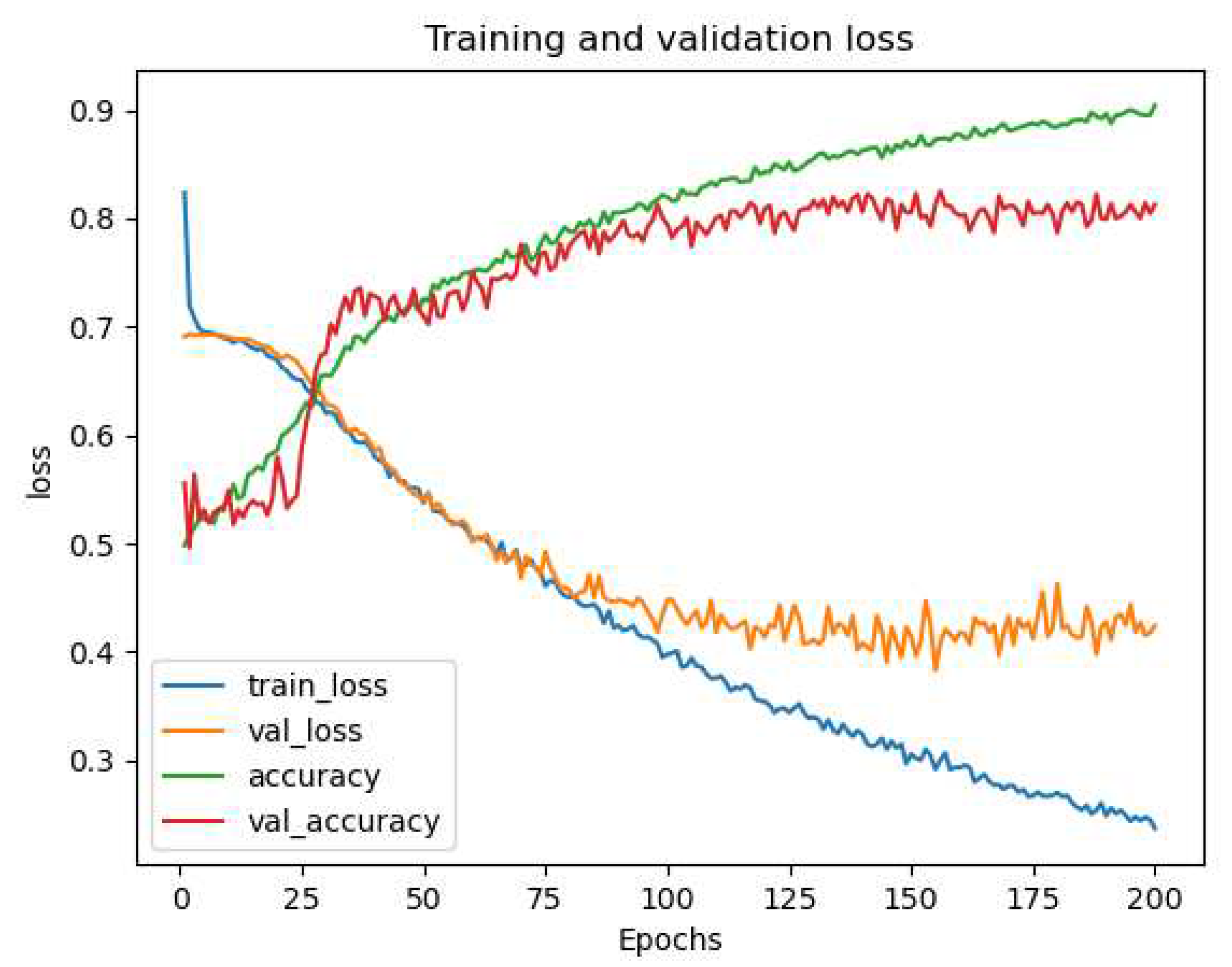
A problem we faced when training and adjusting the model was overfitting. When the model overfits on the dataset, the model learns the features of the training data too well, yet cannot distinguish the class of images in the validation data with as good of a performance as the training data. Our model overfitting on the
dataset is shown in
Figure 5. When the training accuracy is significantly higher than the validation accuracy, and when training loss is signiicantly lower than validation loss, this is a glaring symptom of overfitting.
can be used to be attempt to control overfitting [
26]. This is a process performed before hidden layers where neurons are randomly removed, or dropped, along with their connections. This random neuron dropping forces the model to adapt how it learns features from inputs [
27]. The number of dropped neurons is determined by the user and is a fraction of the neurons. To be more precise, this is not a definite ratio of neurons to be dropped, this is a calculation performed on each neuron, but given a large enough number of neurons, the total number of dropped neurons should be close to the number set by the model creator. A neuron’s dropout chance is simply calculated:
where p is the set dropout value. Usually, this number is below
, which would be roughly half of the neurons in a layer, because the maximum regularization achievable by the regularization parameter
is
. When
, more neurons are dropped, while regularization does not increase [
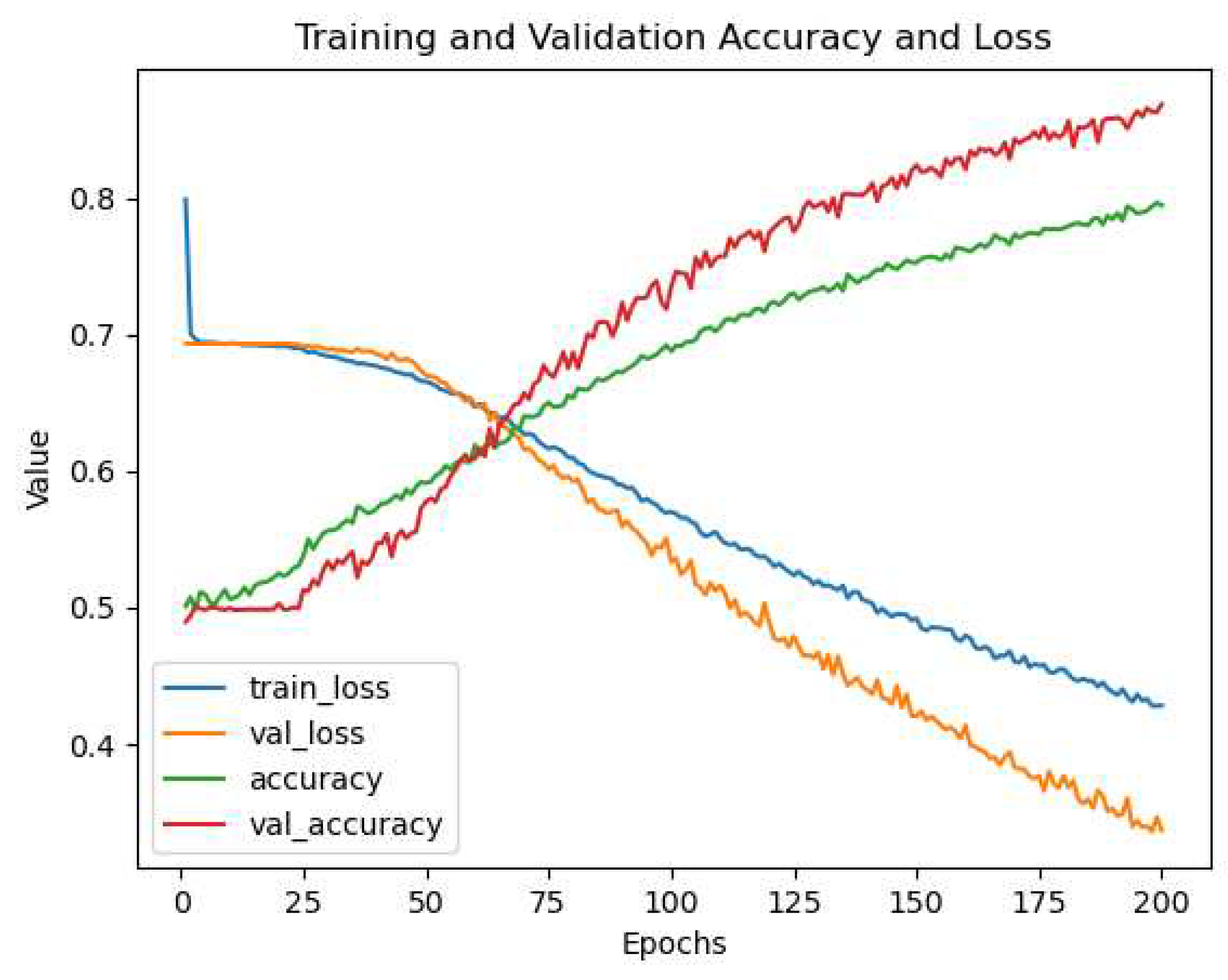
26]. Dropout can also affect the graph of training and validation, where validation and testing performance can be better than training. An example of this is shown in
Figure 6. Since Dropout is only utilized during training, where only a portion of features are used, all features are used during validation and testing.
Another way to mitigate overfitting involved the use of
. Batch normalization is a process performed on a layer that adjusts each “mini batch” against its mean and standard deviation. This will ideally bring each iteration closer to the convergence, where the training and validation metrics of the model are close. Batch normalization is a fairly simply function [
28] shown in Equation (
3).
where
and
are scale coefficient and scale offset, respectively,
x is the input,
is the mean of the mini batch, and
is the standard deviation of the mini batch [
28].
2.5. Histogram of Oriented Gradients Model
The Histogram of Oriented Gradients (HOG) model uses HOG features along with convolutional layers to classify deepfake images. HOG is a computer vision method originally used to detect upright, human poses. The algorithm utilizes binning, similarly to SIFT, to create a histogram of directed orientation, or gradients which are normalized into blocks, which allow for overlapping keypoints. Compared to SIFT, this is a much simpler process that essentially just creates an image of contours and edge data that can be used as feature data.
-
is an open library that contains the function
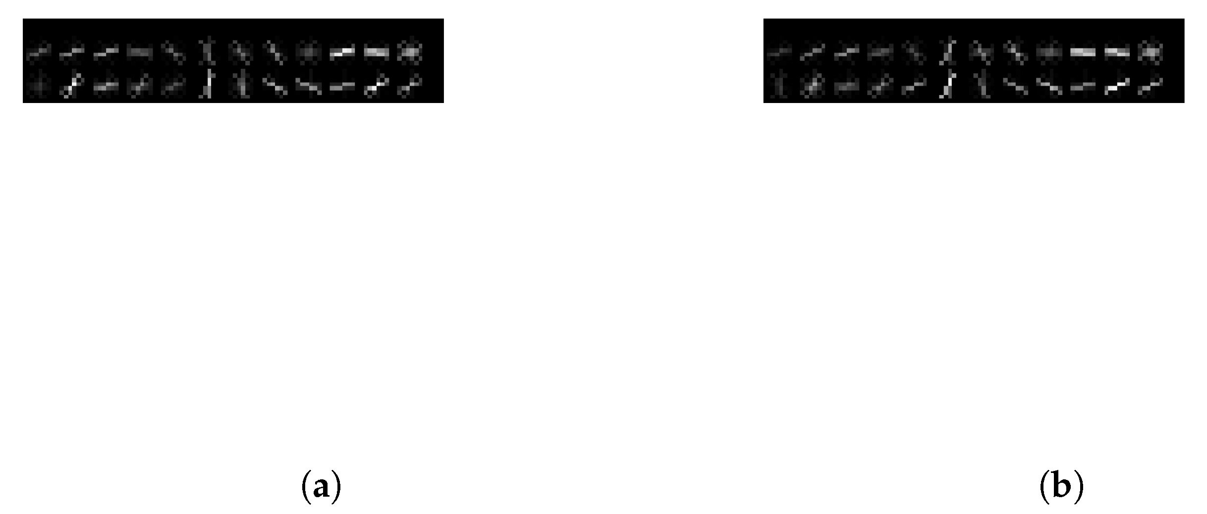
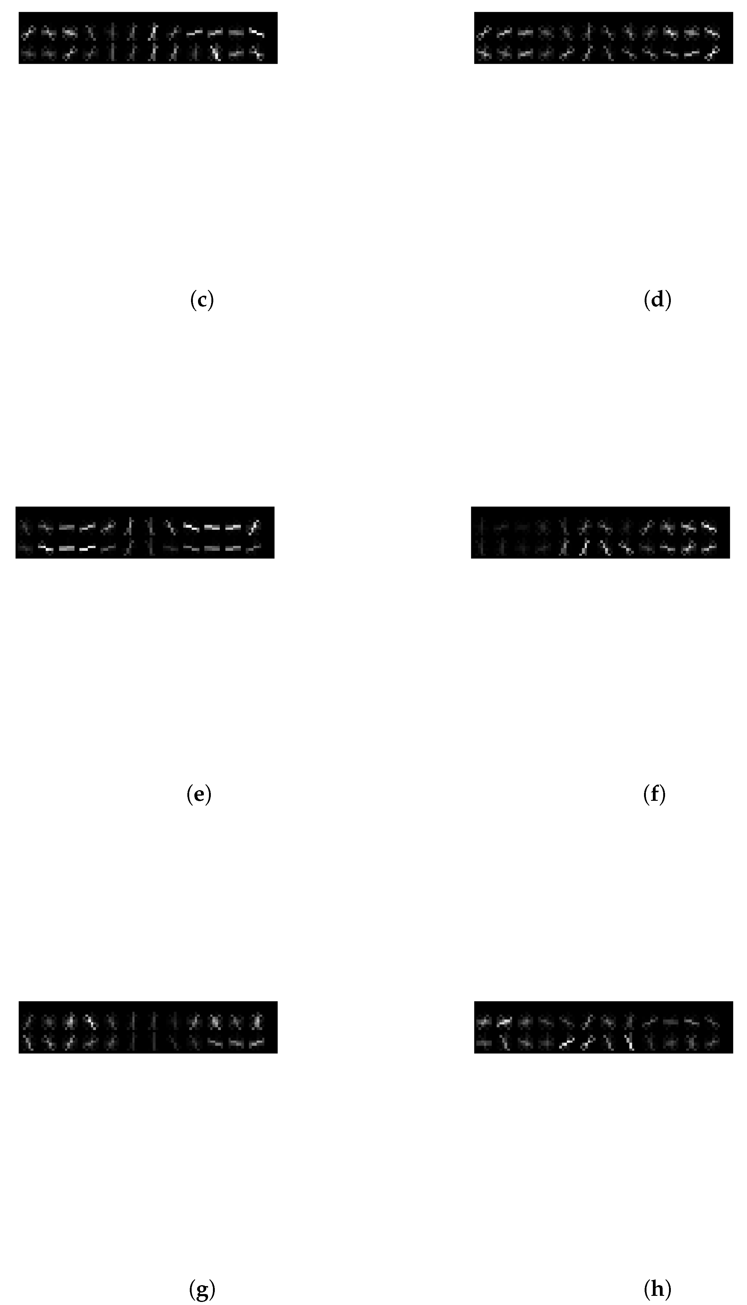
, which returns HOG features and the matching HOG image. Sample HOG images that correspond to their matching features are shown in
Figure 7. The HOG image is a gradient-slope representation of the original image. The initial research [
17] on the HOG algorithm relied on image data of humans standing walking, or in other similar, upright poses - these images were resized to width and height
since the performance of feature extraction is impacted by the input image dimension ratio. The
ratio is not strictly retained, but the orientation is retained, and the ratio loosely retained. Our eye data, which is width and height
is rotated 90clockwise before using it as input for the
function. The features are then returned as a
-array along with corresponding images with focus on the gradients. Only the array is used. The feature data is used as input to convolutional layers. We use convolutional blocks without pooling layers since the feature data only represents itself, without much bearing on neighboring data. The HOG model consists of only two convolutional blocks, where the first convolutional layer has 32 filters and the second has 64 filters. We, again, use two final dense layers with 128 neurons in the first layer and one neuron in the final, classifying layer. The HOG features are saved into a
and saved onto the hard drive for later use with the ensemble model, and also to save preprocessing time during debugging and multiple training iterations with the same data.
2.6. Scale-Invariant Feature Transform Model
The Scale-Invariant Feature Transform (SIFT) model uses SIFT features along with convolutional layers to classify deepfake images. SIFT is a computer vision method used for object- and biological marker detection, object tracking, and edge detection. SIFT uses a scale space to generate keypoints using the Difference of Gaussian. These keypoints are then taken, along with its neighborhood, to create a gradient magnitude and direction. From the magnitude and direction, the SIFT function then places these keypoints into bins, forming a histogram of gradients, similar to Histogram of Oriented Gradients. We now have a location, scale, and orientation for the keypoints, they can be detected across images regardless of changes in the location, size, or rotation. This essentially provides object detection features. Comparatively, SIFT is an extension of HOG, where normalized HOG features are generated based on sections within the input image.
contains the library
which returns keypoints and descriptors using the SIFT algorithm [
16] in a three step process:
extracts keypoints and descriptors to store in two stacked arrays,
use
k-means clustering to focus on the centers of the features which will be be used for,
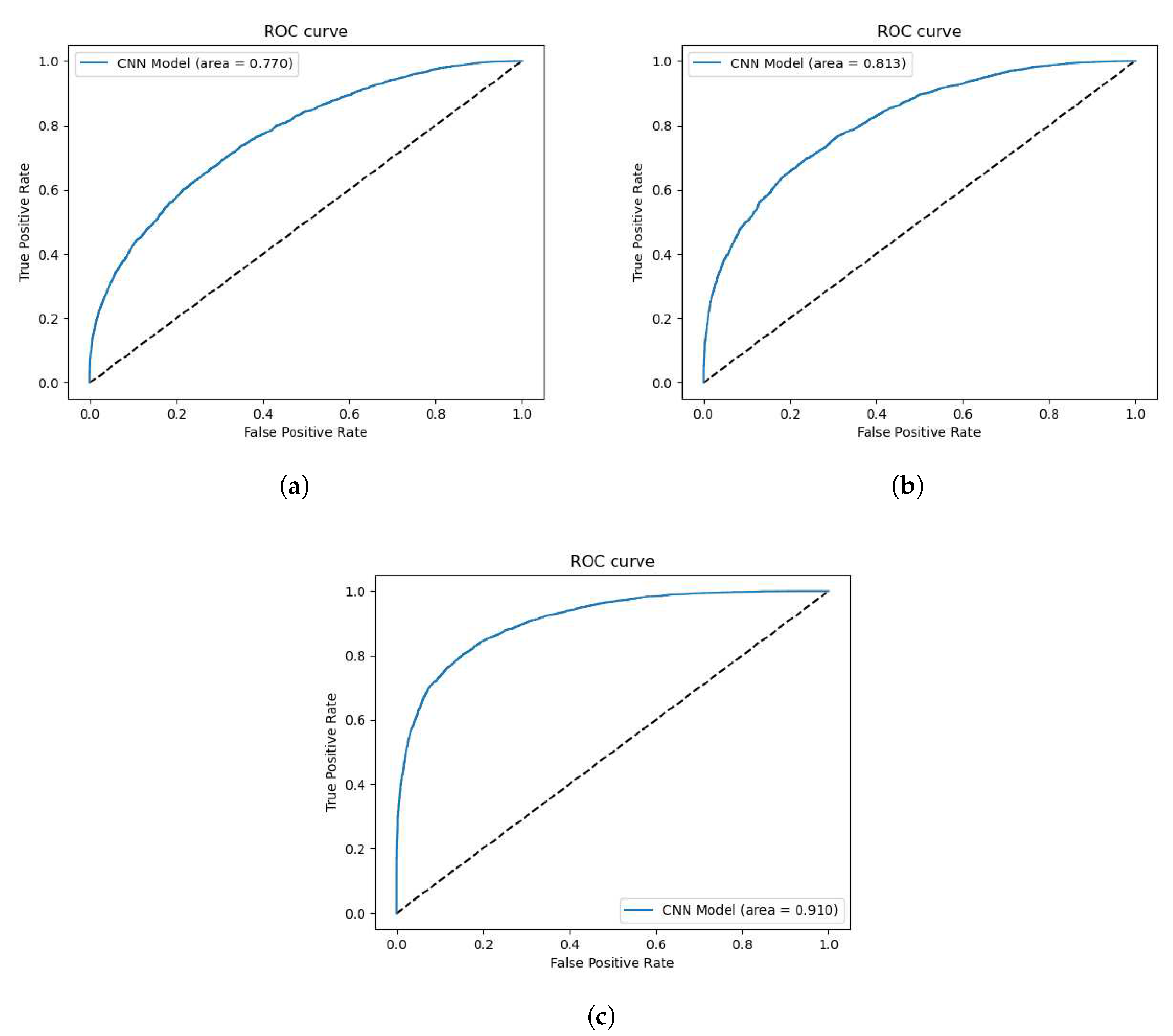
a bag-of-features approach to represent the features and descriptors. After the features are extracted, these are used as input to convolutional layers. Similar to the previous CNN model, this model consists of convolutional blocks, but without pooling layers. Pooling layers are useful to generalize image data and reducing spatial resources and requirements, but it comes at the cost of fine data. For example, averaging sections of pixel data will still result in an image that is recognizable, but not as sharp. This cannot be done with SIFT feature data because extracted feature data does not have much of a relation to the previous or successive data. A comparison of Area under Curve values from the SIFT model using pooling layers is shown in
Figure 8. Max- and Average Pooling layers correspond with a reduction in classification performance, with Max Pooling negatively affecting performance more than average. Max Pooling produced an AUC value of
, Average Pooling produced an AUC value of
, and finally, without pooling layers, the AUC value was
. The SIFT model consists of seven convolutional blocks, where the first two convolutional layers have 32 filters, the next four layers have 64 filters, and the last convolutional layer has 128 filters. The model then has two final dense layers, one with 128 neurons and the final classifying layer with one neuron. The SIFT features are saved into a
and saved onto the hard drive for later use with the ensemble model, and also to save preprocessing time during debugging and multiple training iterations with the same data.
2.7. Ensemble Model
Finally, we create an ensemble model consisting of the previously created models as submodels, or branches, to combine their predictions before further training. Ensemble models typically take one of three forms: bagging, stacking, or boosting. Bagging involves training many models of the same algorithm on a smaller portion of the total dataset, and performing some decision strategy on the many outputs. Stacking involves using different model algorithms on the same input data, then performing some decision strategy on the outputs. Boosting sequentially places models that try to correct the previous model’s prediction errors. In this paper, we discuss our stacked ensemble model. Previously, the models were classifying images based on features specific to that computer vision method of feature extraction, CNN, SIFT, and HOG. With the ensemble, the model will train on the collective extracted features of CNN, SIFT, and HOG per image to increase complexity of the input data. By providing more types of different features, the model would have a larger amount of information to aid in classification.
Figure 9 shows the architecture of the ensemble model with the stacked submodels.
The previously created models share the architecture of the final two dense layers after a flatten layer which makes concatenating their outputs easier. The output of each branch’s flatten layer is concatenated before a dense layer of 128 neurons and a final, classifying layer with one neuron. Also the learning rate was reduced to
to help prevent the model from getting stuck at local minima. When this happens, the model would stop learning, loss and accuracy would remain the same. The architecture of the ensemble model is shown in
Figure 9.
2.8. Training Parameters
The models were trained for 200 epochs with batch size 64. The model was also trained again for a longer period of 400 epochs on the dataset. We also use k-fold cross validation, with a k value of 5 and 10. Ideally, is more robust to verify training and prediction metrics, but memory restraints caused the ensemble model to have to use .
Figure 1.
Visualization of periocular region extraction. Red: MTCNN landmark location. Yellow: Bounding box based on Red. Black: Padded bounding box based on Yellow.
Figure 1.
Visualization of periocular region extraction. Red: MTCNN landmark location. Yellow: Bounding box based on Red. Black: Padded bounding box based on Yellow.
Figure 2.
Sample original, unaltered periocular images used as source for the dataset.
Figure 2.
Sample original, unaltered periocular images used as source for the dataset.
Figure 3.
Sample altered, deepfake periocular images used as source for the dataset.
Figure 3.
Sample altered, deepfake periocular images used as source for the dataset.
Figure 4.
The standalone CNN model used to generate metrics for comparison against SIFT and HOG feature extraction methods.
Figure 4.
The standalone CNN model used to generate metrics for comparison against SIFT and HOG feature extraction methods.
Figure 5.
An example of our model overfitting on the dataset.
Figure 5.
An example of our model overfitting on the dataset.
Figure 6.
An example of our model having significantly better validation performance than training performance on the dataset.
Figure 6.
An example of our model having significantly better validation performance than training performance on the dataset.
Figure 7.
Sample HOG eye images. Images (a–d) are original, real images. Images (e–h) are deepfake images. Samples from DeepFakeDetection dataset.
Figure 7.
Sample HOG eye images. Images (a–d) are original, real images. Images (e–h) are deepfake images. Samples from DeepFakeDetection dataset.
Figure 8.
Figures from SIFT model. (a) ROC AUC with , (b) ROC AUC with , (c) ROC AUC without Pooling.
Figure 8.
Figures from SIFT model. (a) ROC AUC with , (b) ROC AUC with , (c) ROC AUC without Pooling.
Figure 9.
Layered visualization of the multichannel ensemble model.
Figure 9.
Layered visualization of the multichannel ensemble model.
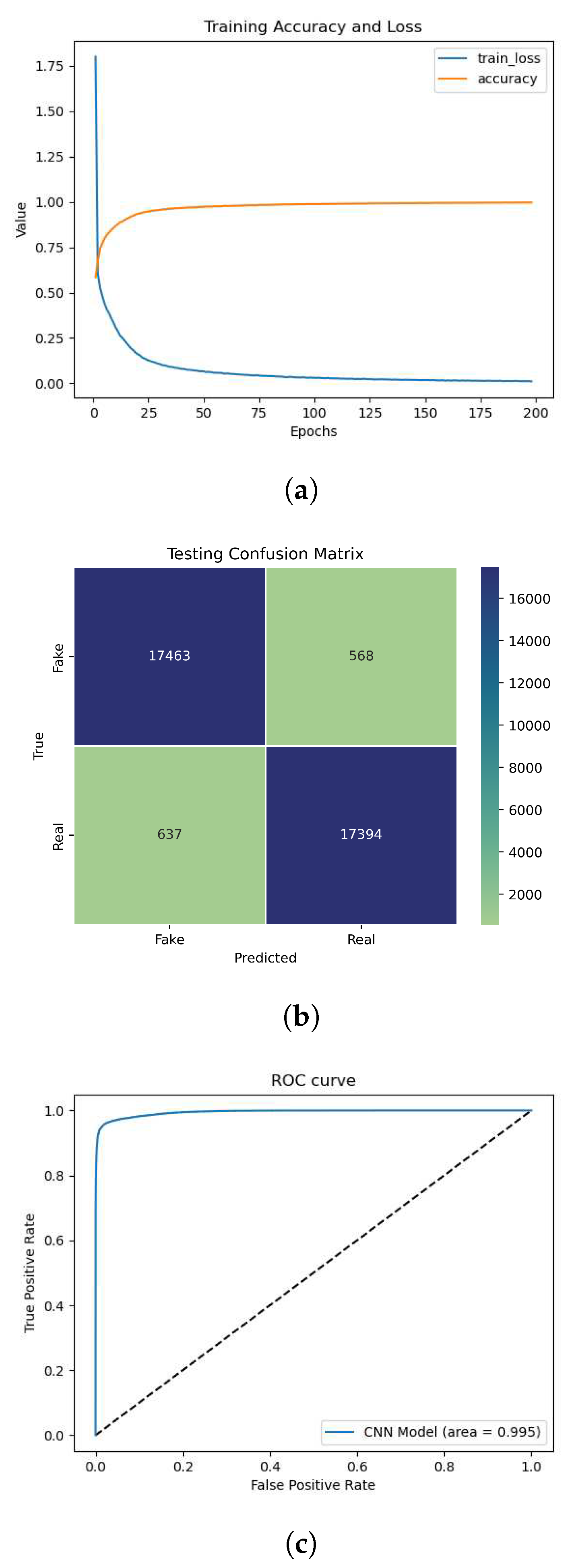
Figure 10.
(a) Training curve, (b) Confusion Matrix, (c) ROC.
Figure 10.
(a) Training curve, (b) Confusion Matrix, (c) ROC.
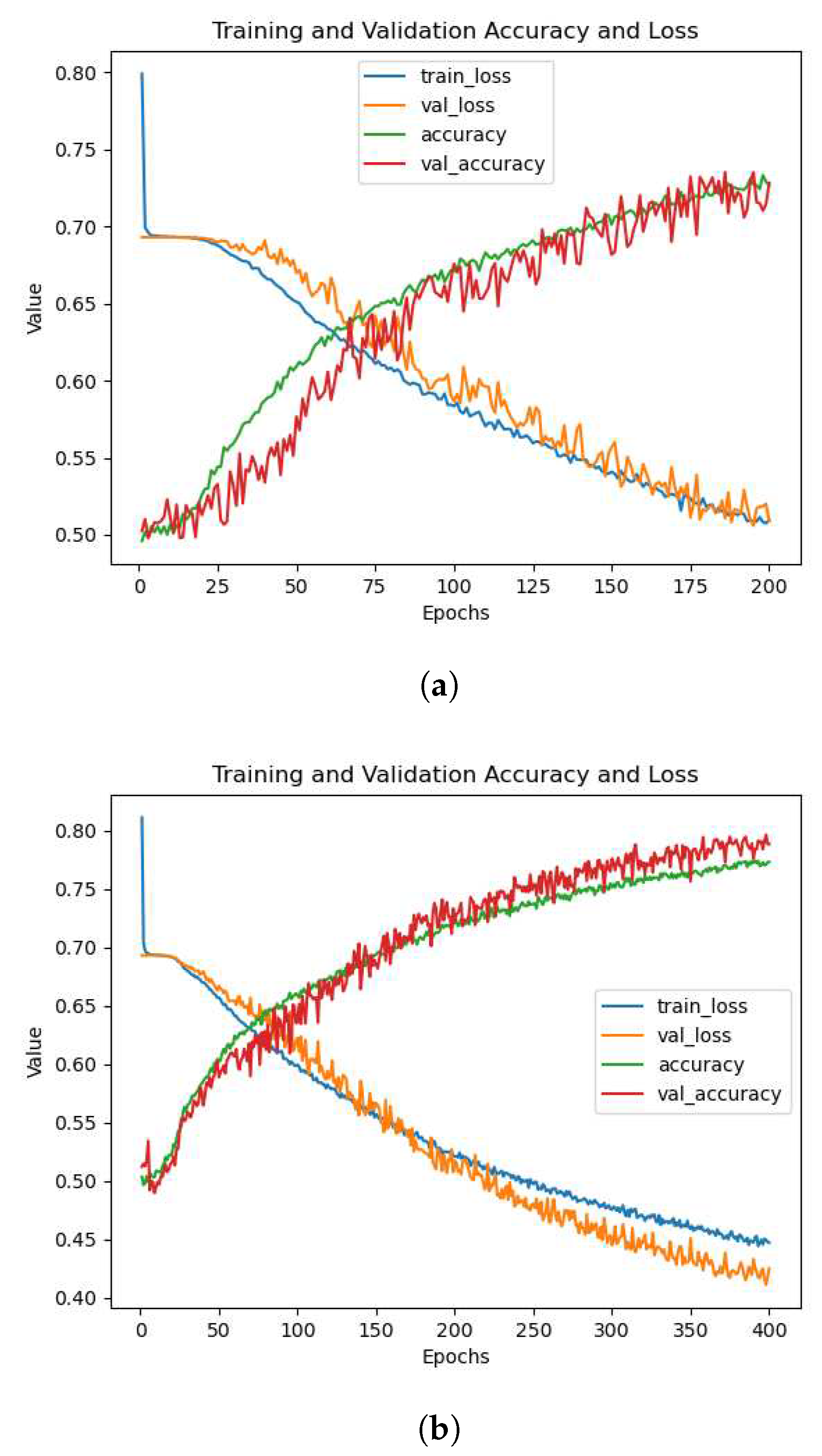
Figure 11.
Figures from training on the dataset. (a) at 200 epochs, (b) at 400 epochs.
Figure 11.
Figures from training on the dataset. (a) at 200 epochs, (b) at 400 epochs.
Table 1.
Training and Testing split
Table 1.
Training and Testing split
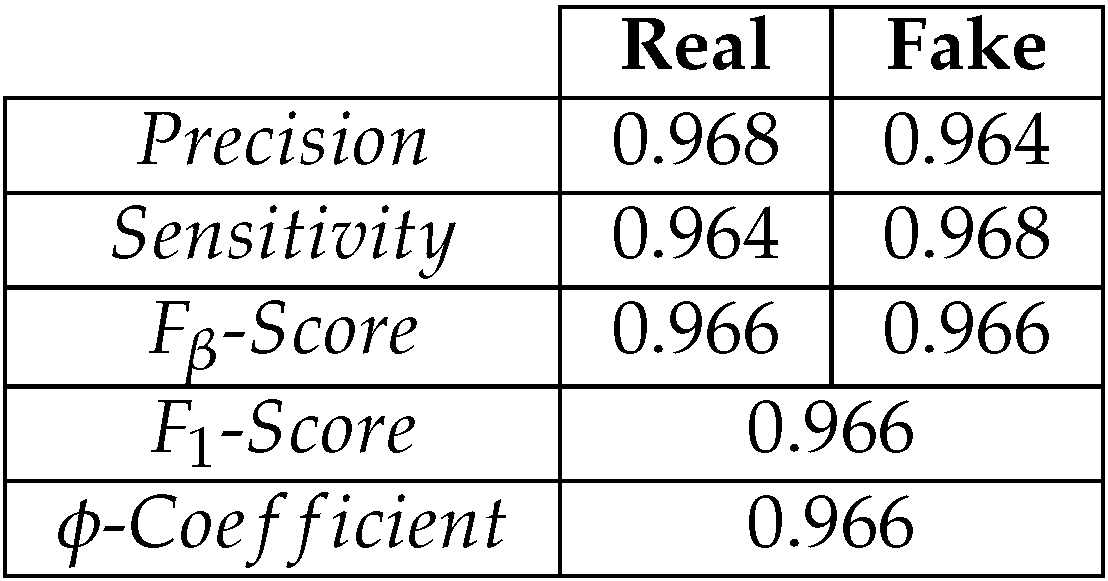
Table 2.
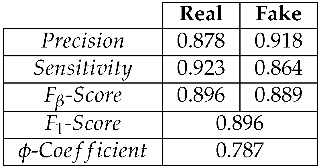
Predictions on a test set from .
Table 2.
Predictions on a test set from .
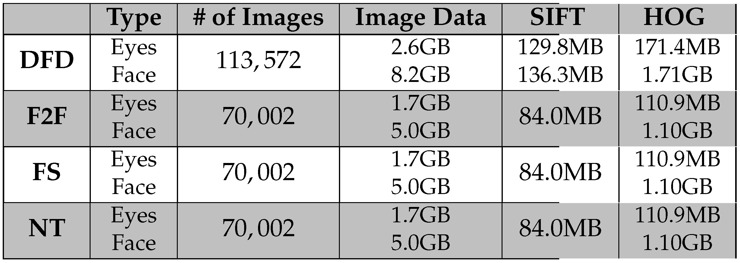
Table 3.
Sizes of the various image and feature datasets used to compare the performance of the ensemble model.
Table 3.
Sizes of the various image and feature datasets used to compare the performance of the ensemble model.
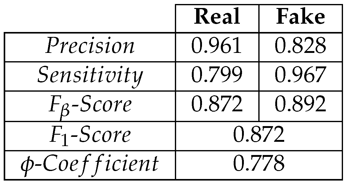
Table 4.
Predictions on a test set from .
Table 4.
Predictions on a test set from .
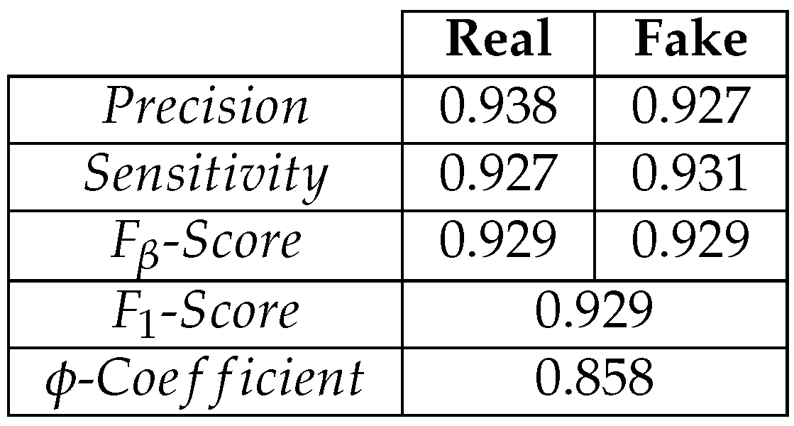
Table 5.
Predictions on a test set from .
Table 5.
Predictions on a test set from .
Table 6.
Predictions on a test set from .
Table 6.
Predictions on a test set from .
