
Submitted:
15 February 2023
Posted:
20 February 2023
You are already at the latest version
Abstract
This research work presents the nonlinear control framework to estimate and reject the mismatched lumped disturbances acting on the nonlinear uncertain system. It is an unfortunate fact that the conventional Extended State Observer (ESO) is not capable to estimate the mismatched lumped disturbance and its derivative simultaneously for the systems. Also, the basic ESO is only suitable for systems with Integral Chain Form (ICF) structure. Similarly, the conventional Feedback Linearizing Control (FLC) approach is not robust for stabilizing the systems in the presence of disturbances and uncertainties. Hence, the nonlinear control framework is proposed to overcome the above issues which are composed of, (a) Dual Extended State Observer (DESO), and (b) DESO based FLC. The DESO provides information on the unmeasured state, mismatched disturbance, and its derivative. While the DESO-FLC utilizes the information from DESO to counter the effect of such disturbances and to stabilize the nonlinear systems around the reference point. The detailed closed-loop analysis is presented for the proposed control framework in the presence of lumped disturbances. The performance robustness of the presented design has been validated for the third order, nonlinear, unstable, and disturbed Magnetic Levitation System (MLS). The results of the DESO-FLC approach are compared with the most popular Linear Quadratic Regulator (LQR) and nonlinear FLC approaches based on the integral error criterion and the average electrical energy consumption.
Keywords:
Extended State Observer
; Feedback Linearizing Control
; Mismatched Disturbance
; Nonlinear System
; Stability Analysis
; Lumped Disturbances
1. Introduction
Modern control systems are most of the time affected by one or more irregularities like parameter uncertainties, unmodeled dynamics, nonlinearities, and external disturbances. In general, the combined effect of such irregularities is termed as Lumped Disturbance [1]. The feed-forward compensation is one of the most common approaches to compensate the effect of measurable/predictable disturbances. In day-to-day applications, it is very difficult to measure/predict the individual effect of such disturbances which restricts the usage of the feed-forward compensation. This unfortunate reality has increased the popularity of lumped disturbance estimation and rejection methodologies. In the past two decades, various approaches have been reported to estimate such disturbances. This includes, the new Extended State Observer (nESO)[2], the Hybrid Extended State Observer (HESO)[3], the Disturbance Observer (DOB)[1], the Generalized DOB (GDOB)[4], the Equivalent Input Disturbance (EID)[5], the Active Disturbance Rejection Control (ADRC)[6]. Among these approaches, the Extended State Observer(ESO) is a widely used method due to the requirement of minimal system information. The ESO is the backbone and fundamental component of the Active Disturbance Rejection Control(ADRC) methodology [6]. These features have rapidly boost-up the feasibility, and applicability of the ESO based Control (ESOBC) methodologies [7]. Majority of the control systems, based on the applied control input signal(i.e., ), the lumped disturbance may be classified as matched disturbance, and mismatched disturbance [8]. The matched disturbance and control input signals enter the systems via the same channel. Therefore, the matched disturbance is easy to estimate and reject compared to the mismatched disturbance 9]. In the beginning, the ESO was developed for estimating the matched type of lumped disturbance. Further, this is applicable for the systems with the Integral Chain Form (ICF) type of canonical structure [10]. It may not be possible or feasible for each system to transform into such ICF structures [11]. These above discussed limitations of ESO have encouraged the research community to upgrade the functionality of ESO. Further, the ESO methodology has been re-designed to tackle the mismatched lumped disturbances with or without ICF structure as, the Generalized Extended State Observer (GESO) [12], the Novel Extended State Observer (NESO) [13], the Enhanced Extended State Observer (EESO)[14], Predictive ESO(PESO) [15], ESO-SMC with backstepping [16], ESO based adaptive constraints control [17], and many more. Once, the mismatched disturbance is estimated, the next crucial task is to design the disturbance rejection control structures. Till date, a variety of control structures have been designed and implemented using the information from the ESO. The most popular structures include Sliding Mode Control(SMC) [18,19], Feedback Linearizing Control(FLC) [20,21], Active Disturbance Rejection Control(ADRC)[22], Anti-Disturbance Control [23], etc.
Most of the above mentioned ESO based control schemes have been designed and implemented for the lower order uncertain systems(i.e., order up to second order). However, in many recent articles [24,25], the Disturbance Observer Based Control(DOBC) schemes have been designed for the higher-order uncertain systems(i.e., order greater or equal to three). The majority of the above mentioned articles have utilized the FLC schemes integrated with the ESO or the Disturbance Observer(DO) to estimate and to suppress the mismatched disturbances. But, the structural limitations of the FLC like state transformation [26] may restrict the usage of ESO based FLC schemes. Most of the Disturbance Observer(DO) approaches including the ESO may be insufficient to provide the information of the first derivative of the lumped disturbances [21,25]. Hence, the DO or ESO based FLC structure may only apply for the limited no. of applications.
Hence, to broaden the applicability of the FLC in practical applications, we have introduced the Dual Extended State Observer Based FLC(DESO-FLC) approach. The novel contribution of this paper is summarized as follows:
- The designed control structure has been validated via simulation for the third-order uncertain Magnetic Levitation System(MLS) to estimate and suppress the combined effect of, the external payload disturbance, the parametric uncertainties.
- The convergence analysis has been carried out for the DESO-FLC based uncertain systems.
- Performance of the proposed design has been compared with the most popular LQR and FLC approaches for diverse operating conditions using the integral error criterion (i.e., ITAE, ISE).
The structure of the paper is organized as follows. In Section 2, preliminaries of the conventional ESO based feedback linearizing control is discussed. Section 3 presents the detailed problem formulation. Section 4 represents the foundation and design of the proposed Dual Extended State Observer Based Control (DESOBC) with the FLC approach. In Section 5, simulation results are presented for the nonlinear, unstable, uncertain, and disturbed Magnetic Levitation System (MLS) using the proposed technique. Finally, the concluding observations are summarized in Section 5.
2. Preliminaries
In this section, the basic structure and algorithm for Extended State Observer(ESO) and Feedback Linearizing Control(FLC) methods are discussed. Till date, these methods have been widely used for a broad range of practical applications.
2.1. Extended State Observer (ESO)
The concept of ESO was first introduced by Han [27] to observe the disturbance as an extended state. The conventional order Single Input Single Output(SISO) uncertain system with Integral Chain Form (ICF) is presented as follows [12]:
where is the state vector with ,,..., are states, u is a control input, y is a controlled output, is an external disturbance, is a coefficient of the control input, and presents the lumped disturbance. This disturbance is tackled by considering it as one of the extended states () of the system as follows:
The above-mentioned dynamics in are transformed by to estimate as well as any unmeasured states. The Nonlinear ESO(NESO) with the bounded conditions, i.e. and are described as follows [28,29]:
where is the output estimation error, and ), are the linear and nonlinear gains of the NESO. The standard expression for with fine tuning of parameters (i.e. and ) are expressed with as follows [27,30]:
It has been shown that the error dynamics of the NESO converge under the bounded conditions and the proper selection of the gains (i.e. and ) [7]. Hence, the NESO based control law (u) can be written by .
Here, and are the state-feedback gain vector and reference gain respectively with the reference value (r). For brevity, in this manuscript, variables are presented only by the symbol without the function of time (i.e. is presented by x). It has been reported that the disturbance considered for the ESO (i.e. ) is a class of "Matching Lumped disturbance". To get the idea of such a class of disturbance, the uncertain SISO system in is presented in a more generalized form in as shown below [10]:
xx[Lumped disturbance [12]] A class of generalized disturbance which is the combination of external disturbances, unmodeled dynamics, parameter variations, and complex nonlinear dynamics is so-called the Lumped disturbance.
yy[Matching Lumped disturbance [12]] A class of Lumped disturbance with , is so-called the Matching Lumped disturbance.
2.2. Feedback Linearizing Control (FLC)
In general, the affine dynamics for the order nonlinear SISO system is described by the following equations [31].
where is the state vector with ,,..., are states, u is a control input, y is a controlled output, , and are the smooth vectors presenting the states, input, and output respectively. As described in [32], it is always possible to transform (i.e. ) the nonlinear dynamics of (8) in the canonical form if the relative degree equals the order of the system using the Lie algebra as shown below [33]:
New transformed dynamics of (8) are described using (9) as follows:
Hence, following nonlinear control law integrated with the state-feedback control presented in (11) or (12) would suppress the effect of nonlinearities (i.e., , , ) and stabilize the system around the reference value (r).
OR
Here, and are the state-feedback gain vector and reference gain respectively as discussed in the earlier section.
3. Problem Statements
The brief about the conventional FLC approach has been discussed in the previous section for the nonlinear SISO systems. It has been shown that the FLC is capable of suppressing the effect of nonlinearities from the output of the systems [31]. It is also possible to stabilize and track the considered nonlinear system using the FLC. The application of ESO in estimating the lumped disturbances as well as unknown states is also briefly explained in the previous section. Based on the structure of the FLC and the ESO, the following problem statements have been formulated.
- The FLC approach may not provide robust performance in the presence of lumped disturbances. The addition of integral action (i.e., FLC+I) can be seen as one of the solutions to suppress the constant or the slow-varying disturbances [4]. However, the nominal performance of the uncertain system may be degraded using such integral action when there is no disturbance [29].
-
To handle such lumped disturbances for the second order nonlinear systems, the FLC integrated with the Disturbance Observer (i.e, FLC+DO) has been proposed in [21]. Such a method may not suitable for the following type of higher-order nonlinear systems in (13). For brevity, the higher-order system is presented by (14) with in this research.OR
-
The group of uncertain systems presented by (14) has been affected by the multiple nonlinearities (i.e, , , ) and the mismatched lumped disturbance (i.e, ).
- (a)
- Nonlinear terms can be compensated from the output using the FLC methods. Now, the conventional ESO method can be utilized to tackle the matched lumped disturbances for the systems with ICF structure [12]. However, the considered system is affected by the mismatched lumped disturbance and does not follow the ICF structure. Hence, neither the conventional ESO method [27] nor the FLC+DO method [21] may provide robust performance.
- (b)
-
The considered third-order system in (14) can be expressed in the input-output form using the derivatives of output as follows:Hence, based on (15), to compensate for the unwanted effect of the nonlinearities and the disturbances together using the conventional FLC approach, it is recommended to estimate the unknown states, the mismatched lumped disturbance () and it’s first derivative (). For the higher-order systems (i.e, ), estimation of the second and higher order derivatives is required.
- Finally, to get rid of the above-stated problems, it is necessary to investigate and expand the individual functionalities of the FLC and the ESO for the higher-order ( for this research) uncertain systems. In such situations, the usage of ESO methods is more favorable in estimating the unknown states, disturbances, and their higher-order derivatives simultaneously [12,19,21,25,34].
4. Dual Nonlinear Extended State Observer Based FLC (DESO-FLC)
This section is designed to address the problems associated with the conventional ESO (nonlinear type) and FLC in handling the mismatched lumped disturbance for the uncertain systems in (14). The proposed research in this section is presented in two subsections: Dual ESO (DESO), and DESO based FLC (DESO-FLC) respectively. The design of such modified structures is valid under the following assumptions.
zAssumption [12] For most of the real-time physical uncertain systems, and its higher-order derivatives can be assumed as the bounded signals. i.e., , .
yzAssumption [26] The known smooth function () in (14) is continuously differentiable and can be further expressed using the partial derivatives as follows:
4.1. Dual Extended State Observer (DESO)
In this section, the unknown state (), mismatched lumped disturbance (f(x,d(t),t)) and its first derivative () are estimated simultaneously using the conventional nonlinear ESO. The reduced-order dynamics in (14) can be presented as follows:
It is possible to present the lumped disturbance using a neutralized dynamic model with and as follows [35]:
where
Now, cascading the reduced-order dynamics in (17) and the disturbance model dynamics in (19), the new state vector () for the DESO can be written as follows:
Hence, the dynamics of the Dual ESO with known information vector () can be described as follows:
where
yyAssumption The Dual ESO presented by (21) has the observable pair ( , ).
Under the Assumption-4 and Assumption-4.1, the unknown states of (21) can be estimated using the Nonlinear ESO (NESO) described earlier in (4) as follows:
Theorem 1.
(Convergence of DESO) Suppose that Assumptions-1, 2, 3 are satisfied. Then the DESO dynamics presented by (23) converge.
4.2. DESO Based Feedback Linearizing Control (DESO-FLC)
Theorem 1.
Suppose that Assumptions-1, 2, and 3 are satisfied and the considered system is feedback linearizable. Then the output (y) in (14) can be stabilized around the reference value (r) using the following DESO-FLC law with and .
Proof.
It is assumed that the considered third order system is feedback linearizable [25]. Hence, it is possible to perform the state transformation described in (9) using and as follows:
As we know, under Assumption-2, the partial derivatives of can be expressed by (16). Hence, using the partial derivatives and (14), the modified transformed vector can be expressed as follows:
Now, implementing the proposed control law (u) into the above dynamics, the following result is obtained.
Here, and are the disturbance estimation error and it’s derivative due to DESO. However, according to Theorem 1, gets an asymptotic convergence such that at , and . Using these results, the following expression is written.
Converting the transformed dynamics back as a function of the output of the original system dynamics, the following differential equation is obtained.
The state feedback gains (i.e., , , ) and the reference gain () can be designed using any appropriate feedback control method such that at ,
Hence, it is proved that output (y) of the considered third order nonlinear system is stabilized around r using the DESO-FLC even under the presence of the mismatched lumped disturbances and nonlinearities. □
5. Practical Application and Results
The Magnetic Levitation System (MLS) is one of the best practical applications to validate the effectiveness of control algorithms. MLS is a class of nonlinear, unstable, and electromagnetically coupled systems with a broad range of practical applications [37,38]. The schematic of voltage-controlled MLS is presented in Figure 1 [37].
Here, the prime objective is to maintain the airgap (x) between the steel ball and electromagnet by manipulating the coil voltage (). The mismatched lumped disturbance for this experiment is the total effect due to the payload disturbance and the uncertain electromechanical parameters (i.e., , ). The voltage-controlled dynamics of MLS with mismatched lumped disturbance () is expressed by the following third-order nonlinear model [39]:
In above nonlinear disturbed state-model, , , are three states of the MLS as ball position (x), ball velocity () and coil current (i) respectively. While, the coil controlled voltage () and the ball position () are the input (u) and output (y) of the MLS. The parameters used for the simulation are mentioned in Table 1[40,41].
Here, the ball position () and the coil current () are measurable information using the position detector and the current sensor respectively. Hence, the nonlinear dynamics of MLS in (33) can be written in the form of DESO with smooth function, . Assumption 3 is true for the MLS such that it is possible to establish the DESO as described in (21). Using the guidelines in [7,42] for the convergence, the parameters are chosen as , and . Using the DESO module, the ball velocity (), the mismatched lumped disturbance, and its first-order derivative can be obtained as ; ; and respectively. After getting the estimation of the unknown states and lumped disturbances, the DESO-FLC law is required to obtain as described in (25). In the case of the MLS, the continuous smooth function and its partial derivatives are presented under Assumption 2 as follows :
where
For the third-order nonlinear disturbed MLS (33), the known smooth functions , and can be written as follows:
Finally, implementing the DESO-FLC law with based on Theorem 2 using the information in (34)-(36) will result into the following transformed dynamic of MLS.
As per the earlier discussion, the estimation of the mismatched lumped disturbance and its derivative converge to the actual information using the DESO such that . Finally, based on the state feedback controller design, the controller gains as and satisfies (32) at . The proposed generalized control algorithm is validated under the following cases of the bounded mismatched lumped disturbances as per Assumption 1 for the MLS. The performance effectiveness of the DESO-FLC approach is compared with the most popular Feedback Linearizing Controller (FLC) and the LQR controller. The LQR controller is designed around the operating position () of m with the following parameters.
5.1. Case 1: Payload Disturbance ()
This is one of the most common lumped disturbances for the MLS. The amount of payload ranges from % of its nominal weight [43]. Hence, in Case 1, the only payload is considered as a mismatched lumped disturbance as +sin, rad/sec.
Such a critical external disturbance and its derivative are estimated using the DESO as shown in Figure 2. It is clearly observed that the proposed algorithm is capable to estimate the payload disturbance in less than 0.1 seconds with negligible transient peak. Also, the rate of change of payload is precisely estimated without any spike or overshoot compared to the filtered derivative of the actual one. Performance of the DESO is also validated in the presence of square and saw-tooth kind of payload disturbances as presented in supporting information in Figure S1 and Figure S2 respectively. For the MLS, 0.001m is the maximum allowable deviation of the ball position from the reference position (r). Therefore, one of the prime duties of the control system is to keep the ball position very near to m from the initial ball position of m.
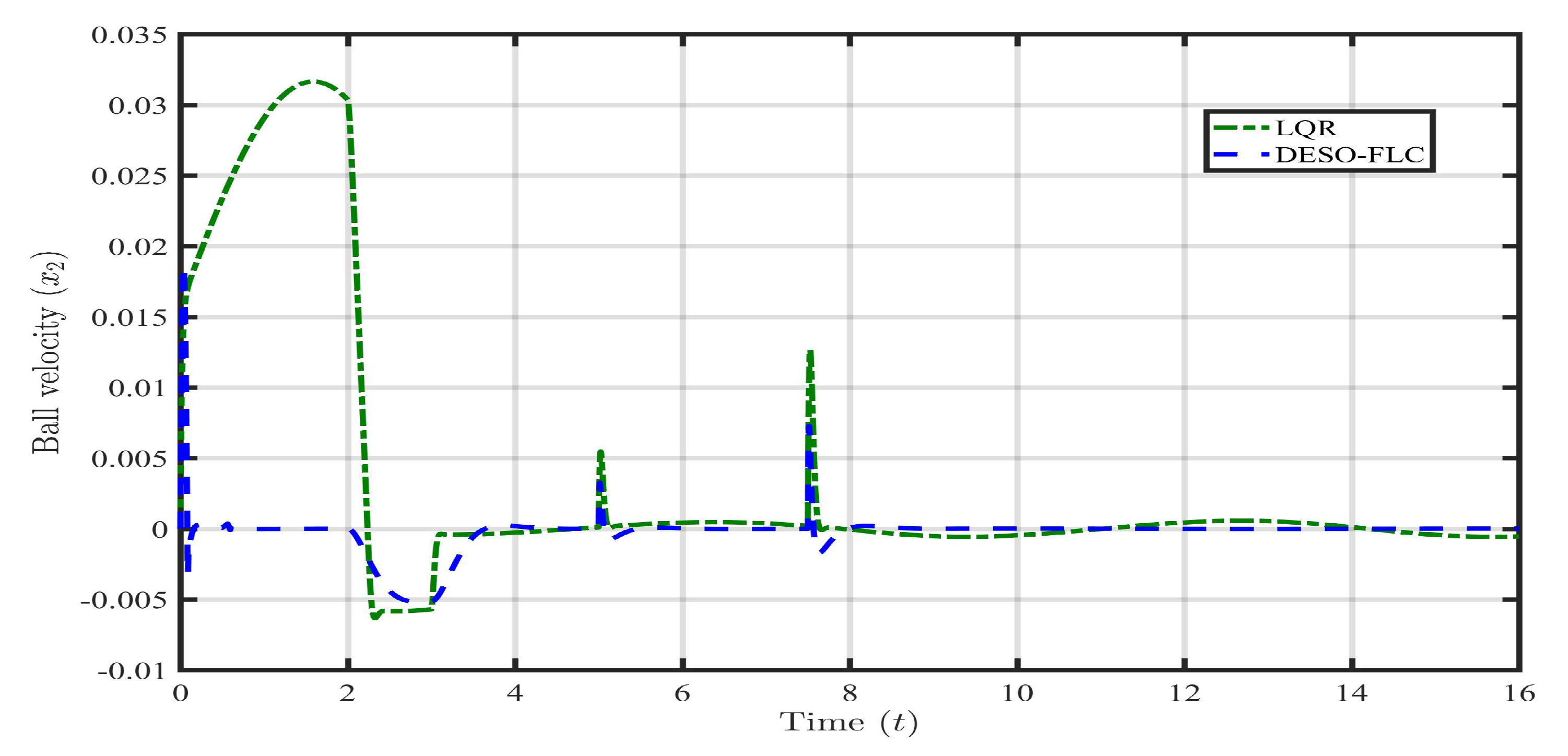
Now, the information on the lumped disturbance and its derivative are available. Hence, the DESO-FLC law is utilized to govern the MLS in the presence of payload disturbance (). The responses of the ball position, ball velocity, coil current, and coil voltage using different control approaches (i.e., FLC, LQR, and DESO-FLC) are presented in the following Figure 3, Figure 4, Figure 5 and Figure 6 It is clearly observed that the conventional FLC is not capable to stabilize the MLS in presence of . The LQR is showing a bounded oscillatory response which is somewhat better than the FLC. However, such continuous up-down movement of the steel ball may cause instability as it is very near to the upper maximum allowable limit. The DESO-FLC is showing a tight, oscillation free, and stable response even in the presence of extreme payload disturbance. It is seen from Figure 5 and Figure 6 that the proposed control approach is optimal in utilizing average coil current (A) and coil voltage ( V) to stabilize the system. In the case of the LQR, these values are 1.41 A and 16.2 V respectively. To evaluate the performance effectiveness, error criteria like Integral Square Error (ISE) and Integral Time Absolute Error (ITAE) have been computed using all three control approaches as shown in Table 2 In these findings, the DESO-FLS have shown the least amount of both integral errors compared to the rest.
5.2. Case 2: Parametric Uncertainty (, )
The second kind of common mismatched disturbance belongs to case 2. Here, the parameters of the systems are uncertain in nature. In the case of the MLS, the parameters associated with the weight and the dimension of the levitation objects are the prime sources of uncertainties [44]. Out of many parameters, the combined effect of uncertain weight () and uncertain electromagnetic constant () are considered in this paper. During the simulation, this lumped uncertainty is applied with the magnitude of 5% and 15% at and seconds respectively. The DESO algorithm is utilized to estimate the total effect of and due to parametric uncertainty as shown in Figure 7.
Similar to case 1, the DESO is smoothly tracking the lumped uncertainty without any unwanted spikes, offset, and distortion. Due to the sudden change in the parameter, there is a negligible overshoot during the transient for 0.1 second. Again, the rate of change of lumped uncertainty is correctly estimated without any spike or deviation compared to the filtered derivative of the actual one. Now, the information on the lumped disturbance is available via the proposed estimator. Hence, the DESO-FLC law can be well implemented to settle the steel ball near the reference value (r) even in the presence of such mismatched parametric uncertainty. The responses of the state variables (i.e., ) and input (u) using various control approaches (i.e., FLC, LQR, and DESO-FLC) are shown in following Figure 8, Figure 9, Figure 10 and Figure 11
Till second, the FLC approach tightly holds the ball position around the reference value. But, when enters into the MLS, the control of FLC is totally disturbed by the lumped parametric uncertainty. Steel ball falls down to the initial position of m with very high steady-state ball velocity of m/s. The LQR has shown quite a good response with a small offset compared to FLC under 5% change in till second. However, when the amount of has increased from 5% to 15% from second, the effectiveness of the LQR has drastically reduced. This results in the large permanent offset (very near to unsafe zone) between the actual ball position () and reference value (r). In the case of the DESO-FLC, the performance effectiveness is maintained throughout the response even in the presence of 5% to 15% parametric changes. At second, the small overshoot followed by negligible undershoot has been observed. But, this is very well accepted for a huge amount of lumped uncertainty. It is observed from Figure 10 and Figure 11 that the FLC has utilized the maximum amount (up to saturation) of electrical quantities to handle the disturbances. The LQR has consumed average coil current (A) and coil voltage ( V) to govern the MLS. However, in the case of the DESO-FLC, these electrical quantities are 1.38A and 15.2V respectively. The Integral Square Error (ISE) and Integral Time Absolute Error (ITAE) have been computed using all three control approaches as shown in Table 3. In these findings, the DESO-FLC has again shown the least amount of both integral errors compared to the rest.
5.3. Case 3: Payload disturbance with Parametric Uncertainty (, , )
This is one of the extreme cases of mismatched lumped disturbances for the MLS. Here, the payload disturbance of case-1 and the parametric uncertainties of case-2 act simultaneously. This kind of extreme internal and external disturbance and its derivative are estimated using the DESO as shown in Figure 12.
Similar to case-1,2, the proposed algorithm is capable to estimate the considered mismatched disturbance very smoothly. There is minor tracking error when . Hence, ± 2 is the maximum allowable mismatched disturbance which can be estimated using the DESO based on Assumption 4. Also, the rate of change of the disturbance is precisely estimated with negligible spike or overshoot compared to the derivative of the actual one.
Figure 13.
Response of steel ball position () in presence of payload disturbance and parametric uncertainties.
Figure 13.
Response of steel ball position () in presence of payload disturbance and parametric uncertainties.
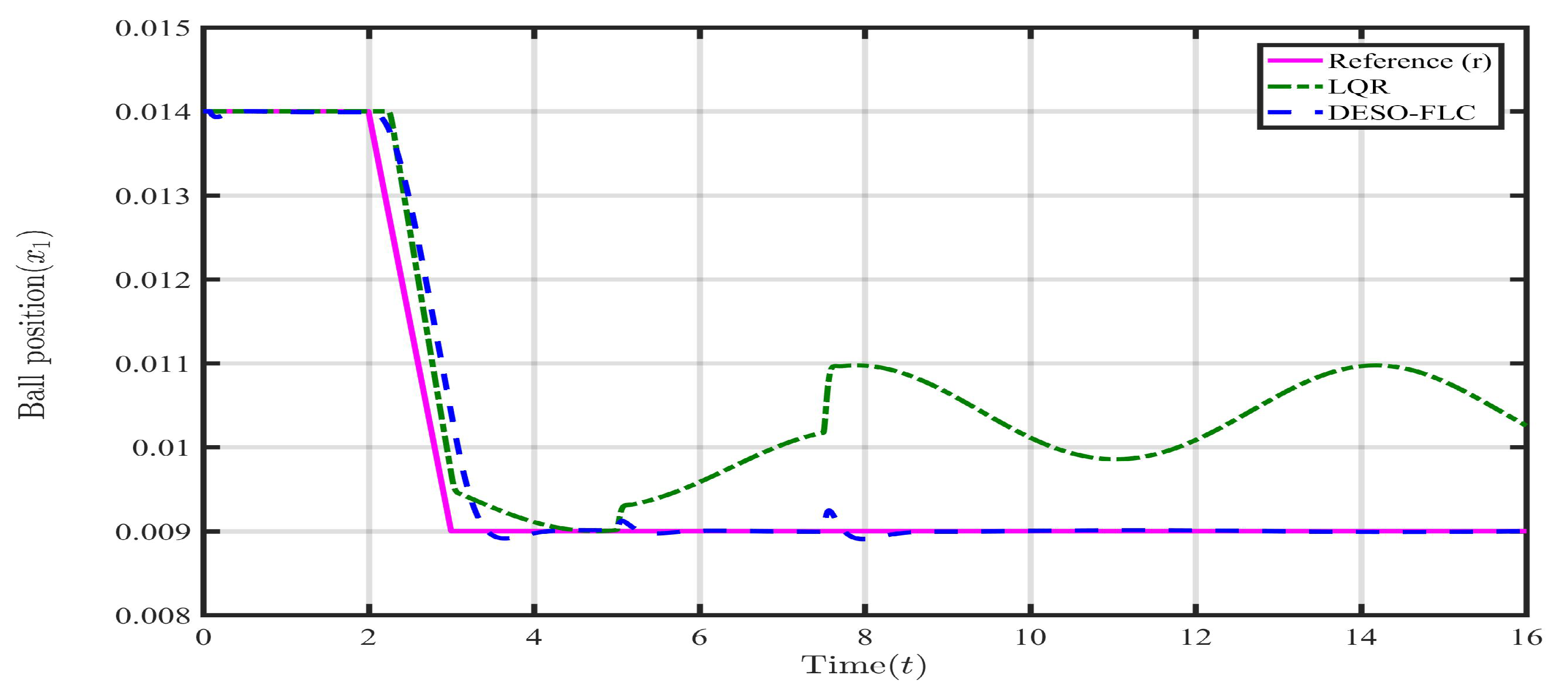
Figure 14.
Response of steel ball velocity () in presence of payload disturbance and parametric uncertainties.
Figure 14.
Response of steel ball velocity () in presence of payload disturbance and parametric uncertainties.
Now, the information on lumped disturbance is available via the proposed estimator. Hence, the DESO-FLC law can be well implemented to settle the steel ball near the reference value (r) even in the presence of such extreme mismatched disturbance. The FLC approach has failed to hold the steel ball within safe limits in case 1 and case 2. Hence, the responses of the state variables (i.e., ) and input (u) using LQR and DESO-FLC are shown in the following Figure 8, Figure 9, Figure 10 and Figure 11.
Till second, both the controllers maintain the ball position within 0.009±0.001 m which is a safe zone. However, for the LQR approach, after , the ball quickly crosses the safe zone and oscillates continuously outside the allowable position which shows the BIBO instability. In practical applications, beyond the safe zone, the electromagnet may not capable to hold the levitating object. This may cause the falling of the object and cause damage. However, the DESO-FLC maintains the ball position and BIBO stability around the reference value (r). It is observed from Figure 15 and Figure 16 that the LQR has consumed a very huge amount of coil current (around A) and coil voltage (around V) to govern the MLS. However, in the proposed design, these electrical quantities are minimal around 1.4A and 16.1V respectively. Also, the Integral Square Error (ISE) and Integral Time Absolute Error (ITAE) have again shown the least amount for the DESO-FLC approach as shown in Table 4.
Hence, it can be stated that the DESO-FLC tackles the mismatched lumped disturbances and stabilizes the steel ball with the least amount of energy consumption.
6. Conclusions
The limitations of the conventional Extended State Observer (e.g. integral chain structure, matching disturbance, etc.) have been compensated by introducing the Dual ESO (DESO). The DESO is capable of estimating the mismatched lumped disturbance (external, internal, or combined) and its derivative simultaneously. We have assumed that the disturbance and its derivative are bounded which is quite obvious. Further, the disturbance rejection capabilities and the performance robustness of the traditional Feedback Linearizing Control approach have been strengthened by proposing the DESO Based FLC (DESO-FLC) approach. The efficacy of the proposed research has been verified via simulation for the Magnetic Levitation System which is a third-order nonlinear, unstable, and disturbed system. We have considered the external payload disturbance with various slow-varying signals (i.e. sinusoidal, saw-tooth, square) and the uncertain parameters (, ) as the mismatched lumped disturbance for the MLS. It has been observed from the theory and the simulation that the proposed DESO-FLC approach is more robust than the LQR and conventional FLC approaches in rejecting the disturbances. Also, the proposed approach has consumed lesser electrical energy and shown the least integral errors (i.e., ISE, ITAE) compared to the rest.
Supplementary Materials
The following supporting information can be downloaded at the website of this paper posted on Preprints.org
Author Contributions
Conceptualization, R.G.; methodology, R.G.; software, R.G.; validation, R.G., D.A., G.S.; formal analysis, R.G. and D.A.; investigation, R.G., D.A. and G.S.; resources, R.G., D.A. and G.S.; data curation, R.G., D.A. and G.S.; writing—original draft preparation, R.G.; writing—review and editing, R.G., G.S.; visualization, R.G. and G.S.; supervision, D.A., G.S. and P.B.; project administration, G.S. and P.B.; funding acquisition, G.S and P.B. All authors have read and agreed to the published version of the manuscript.
Funding
This research received no external funding
Informed Consent Statement
Not applicable
Conflicts of Interest
The authors declare no conflict of interest.
Abbreviations
| ADRC | Active Disturbance Rejection Control |
| DOB | Disturbance Observer |
| DOBC | Disturbance Observer Based Control |
| DESO | Dual Extended State Observer |
| DESOBC | Dual Extended State Observer Based Control |
| DESO-FLC | Dual Extended State Observer Based Feedback Linearizing Control |
| ESO | Extended State Observer |
| FLC | Feedback Linearzing Control |
| ICF | Integral Chain Form |
| ISE | Integral Square Error |
| ISTE | Integral Square Time Error |
| LQR | Linear Quadratic Regulator |
| MLS | Magnetic Levitation System |
| NESO | Nonlinear Extended State Observer |
References
- Chen, W.; Yang, J.; Guo, L.; Li, S. Disturbance-Observer-Based Control and Related Methods - An Overview. IEEE Transactions on Industrial Electronics 2016, 63, 1083–1095. [Google Scholar] [CrossRef]
- Ran, M.; Li, J.; Xie, L. A new extended state observer for uncertain nonlinear systems. Automatica 2021, 131, 109772. [Google Scholar] [CrossRef]
- Gandhi, R.V.; Adhyaru, D.M. Hybrid extended state observer based control for systems with matched and mismatched disturbances. ISA transactions 2020, 106, 61–73. [Google Scholar] [CrossRef] [PubMed]
- Nie, Z.; Wang, Q.; She, J.; Liu, R.; Guo, D. New results on the robust stability of control systems with a generalized disturbance observer. Asian Journal of Control 2019, Online, 1–13. [Google Scholar] [CrossRef]
- She, J.H.; Xin, X.; Yamaura, T. Analysis and design of control system with equivalent-input-disturbance estimation. Proceedings of the IEEE International Conference on Control Applications 2006, 1, 1463–1469. [Google Scholar] [CrossRef]
- Huang, Y.; Xue, W. Active disturbance rejection control: Methodology and theoretical analysis. ISA Transactions 2014, 53, 963–976. [Google Scholar] [CrossRef] [PubMed]
- Guo, B.; Zhao, Z. On the convergence of an extended state observer for nonlinear systems with uncertainty. Systems & Control Letters 2011, 60, 420–430. [Google Scholar] [CrossRef]
- Chen, W.; Guo, L. Analysis of disturbance observer based control for nonlinear systems under disturbances with bounded variation. In Proceedings of the Control 2004, 2004; Vol. 1; pp. 1–5.
- Chen, W.H.; Guo, L. Control of nonlinear systems with unknown actuator nonlinearities. In Proceedings of the IFAC Nonlinear Control Systems; 2004; pp. 1347–1352. [Google Scholar] [CrossRef]
- Chen, W.H.; Li, S.; Yang, J. Non-linear disturbance observer-based robust control for systems with mismatched disturbances/uncertainties. IET Control Theory & Applications 2011, 5, 2053–2062. [Google Scholar] [CrossRef]
- I., W.; K., I. On the active input-output feedback linearization of single-link flexible joint manipulator : an extended state observer approach. IEEE Transactions on Industrial Electronics 2018, pp. 1–9.
- Li, S.; Member, S.; Yang, J.; Chen, W.; Member, S.; Chen, X. Generalized Extended State Observer Based Control for Systems With Mismatched Uncertainties. IEEE Transactions on Industrial Electronics 2012, 59, 4792–4802. [Google Scholar] [CrossRef]
- Xiong, S.; Wang, W.; Liu, X.; Chen, Z.; Wang, S. A novel extended state observer. ISA Transactions 2015, 58, 309–317. [Google Scholar] [CrossRef]
- Castillo, A.; García, P.; Sanz, R.; Albertos, P. Enhanced extended state observer-based control for systems with mismatched uncertainties and disturbances *. ISA Transactions 2018, 73, 1–10. [Google Scholar] [CrossRef] [PubMed]
- Castillo, A.; Santos, T.L.; Garcia, P.; Normey-Rico, J.E. Predictive ESO-based control with guaranteed stability for uncertain MIMO constrained systems. ISA Transactions 2021, 112. [Google Scholar] [CrossRef] [PubMed]
- Wang, P.; Zhang, D.; Lu, B. ESO based sliding mode control for the welding robot with backstepping. International Journal of Control 2021, 94, 3322–3331. [Google Scholar] [CrossRef]
- Xu, Z.; Qi, G.; Liu, Q.; Yao, J. ESO-based adaptive full state constraint control of uncertain systems and its application to hydraulic servo systems. Mechanical Systems and Signal Processing 2022, 167, 108560. [Google Scholar] [CrossRef]
- Ginoya, D.; Shendge, P.; Phadke, S. State and Extended Disturbance Observer for Sliding Mode Control of Mismatched Uncertain Systems. Journal of Dynamic Systems, Measurement, and Control 2015, 137, 074502. [Google Scholar] [CrossRef]
- Hou, L.; Wang, L.; Wang, H. SMC for Systems With Matched and Mismatched Uncertainties and Disturbances Based on NDOB. ACTA AUTOMATICA SINICA 2017, 43, 1257–1264. [Google Scholar] [CrossRef]
- Fuh, C.C.; Tsai, H.H.; Yao, W.H. Combining a feedback linearization controller with a disturbance observer to control a chaotic system under external excitation. Communications in Nonlinear Science and Numerical Simulation 2012, 17, 1423–1429. [Google Scholar] [CrossRef]
- Kayacan, E.; Fossen, T. Feedback linearization control for systems with mismatched uncertainties via distrubance observers. Asian Journal of Control 2019, 21, 1–13. [Google Scholar] [CrossRef]
- Ran, M.; Wang, Q.; Dong, C. Active Disturbance Rejection Control for Uncertain Nonaffine-in-Control Nonlinear Systems. IEEE Transactions on Automatic Control 2017, 62, 5830–5836. [Google Scholar] [CrossRef]
- Guo, L.; Cao, S. Anti-disturbance control theory for systems with multiple disturbances: A survey. ISA Transactions 2014, 53, 846–849. [Google Scholar] [CrossRef]
- Liu, C.; Liu, G.; Fang, J. Feedback Linearization and Extended State Observer-Based Control for Rotor-AMBs System. IEEE Transactions on Industrial Electronics 2017, 64, 1313–1322. [Google Scholar] [CrossRef]
- Kayacan, E.; Peschel, J.; Chowdhary, G. A self-learning disturbance observer for nonlinear systems in feedback-error learning scheme. Engineering Applications of Artificial Intelligence 2017, 62, 276–285. [Google Scholar] [CrossRef]
- Abdul-Adheem, W.; Ibraheem, I. Improved sliding mode nonlinear extended state observer based active disturbance rejection control for uncertain systems with unknown total disturbance. International Journal of Advanced Computer Science and Applications 2016, 7, 80–93. [Google Scholar]
- Han, J. The extended state observer of a class of uncertain systems. in Chinese, Control and Decision 1995, 10, 85–88. [Google Scholar] [CrossRef]
- Gao, Z.; Huang, Y.; Han, J. An alternative paradigm for control system design. In Proceedings of the 40th Conference on Decision and Control; IEEE, 2001; Vol. 5, pp. 4578–4585. [Google Scholar] [CrossRef]
- Li, S.; Yang, J.; Chen, W.; Chen, X. Disturbance Observer-Based Control:Methods and Applications; CRC Press, Taylor & Francis Group, 2014; pp. 1–344.
- Han, J. From PID to active disturbance rejection control. 900 IEEE Transactions on Industrial Electronics 2009, 56, 900–906. [Google Scholar] [CrossRef]
- Gandhi, R.; Adhyaru, D. Novel approximation-based dynamical modelling and nonlinear control of electromagnetic levitation system. International Journal of Computational Systems Engineering 2018, 4, 224–237. [Google Scholar] [CrossRef]
- Ibraheem, I.; Abdul-Adeem, W. An Improved Active Disturbance Rejection Control for a Differential Drive Mobile Robot with Mismatched Disturbances and Uncertainties. In Proceedings of the IEEE; 2017; pp. 7–12. [Google Scholar]
- Freidovich, L.; Khalil, H. Performance recovery of feedback-linearization based designs. IEEE Transactions on Automatic Control 2008, 53, 2324–2334. [Google Scholar] [CrossRef]
- Han, H.; Chen, J.; Karimi, H.R. State and disturbance observers-based polynomial fuzzy controller. Information Sciences 2017, 382-383, 38–59. [Google Scholar] [CrossRef]
- Su, J.; Chen, W.; Li, B. High order disturbance observer design for linear and nonlinear systems. 2015 IEEE International Conference on Information and Automation, ICIA 2015 - In conjunction with 2015 IEEE International Conference on Automation and Logistics, 2015; 1893–1898. [Google Scholar] [CrossRef]
- Guo, B.; Zhao, Z. Active disturbance rejection control: Theoretical perspectives. Communications in Information and Systems 2016, 15, 361–421. [Google Scholar] [CrossRef]
- Gandhi, R.; Adhyaru, D. Modeling of current and voltage controlled electromagnetic levitation system based on novel approximation of coil inductance. In Proceedings of the 2018 4th International Conference on Control, Automation and Robotics (ICCAR); IEEE: Auckland, Newzealand; 2018; pp. 212–217. [Google Scholar] [CrossRef]
- Gandhi, R.; Adhyaru, D. Hybrid intelligent controller design for an unstable electromagnetic levitation system : a fuzzy interpolative controller approach. International Journal of Control and Automation 2019, 13, 735–754. [Google Scholar] [CrossRef]
- Gandhi, R.; Adhyaru, D. Feedback linearization based optimal controller design for electromagnetic levitation system. In Proceedings of the International Conference on Control, Instrumentation, Communication and Computational Technologies (ICCICCT); IEEE: Tamilnadu, India, 2016; pp. 38–43. [Google Scholar] [CrossRef]
- Gandhi, R.; Adhyaru, D. Fuzzy Tuner Based Modified Cascade Control for Electromagnetic Levitation System. In Proceedings of the 2019 Australian and New Zealand Control Conference (ANZCC 2019); 2019; pp. 1–6. [Google Scholar]
- E., J. Quanser magnetic levitation user manual. Technical report, Ontario, Canada, 2012.
- Zheng, Q.; Gao, L.Q.; Gao, Z. On Stability Analysis of Active Disturbance Rejection Control for Nonlinear Time-Varying Plants with Unknown Dynamics. In Proceedings of the 46th IEEE Conference on Decision and Control; 2007; pp. 3501–3506. [Google Scholar]
- Gandhi, R.; Adhyaru, D. Simplified Takagi-Sugeno fuzzy regulator design for stabilizing control of electromagnetic levitation system. In Proceedings of the Innovations in Infrastructure; Springer, Singapore: Ahmedabad, India, 2019; Vol. 757, pp. 1–11. [Google Scholar] [CrossRef]
- Michail, K.; Zolotas, A.; Goodall, R. Optimised sensor selection for control and fault tolerance of electromagnetic suspension systems: A robust loop shaping approach. ISA Transactions 2014, 53, 97–109. [Google Scholar] [CrossRef] [PubMed]
Figure 1.
Schematic of voltage-controlled MLS.
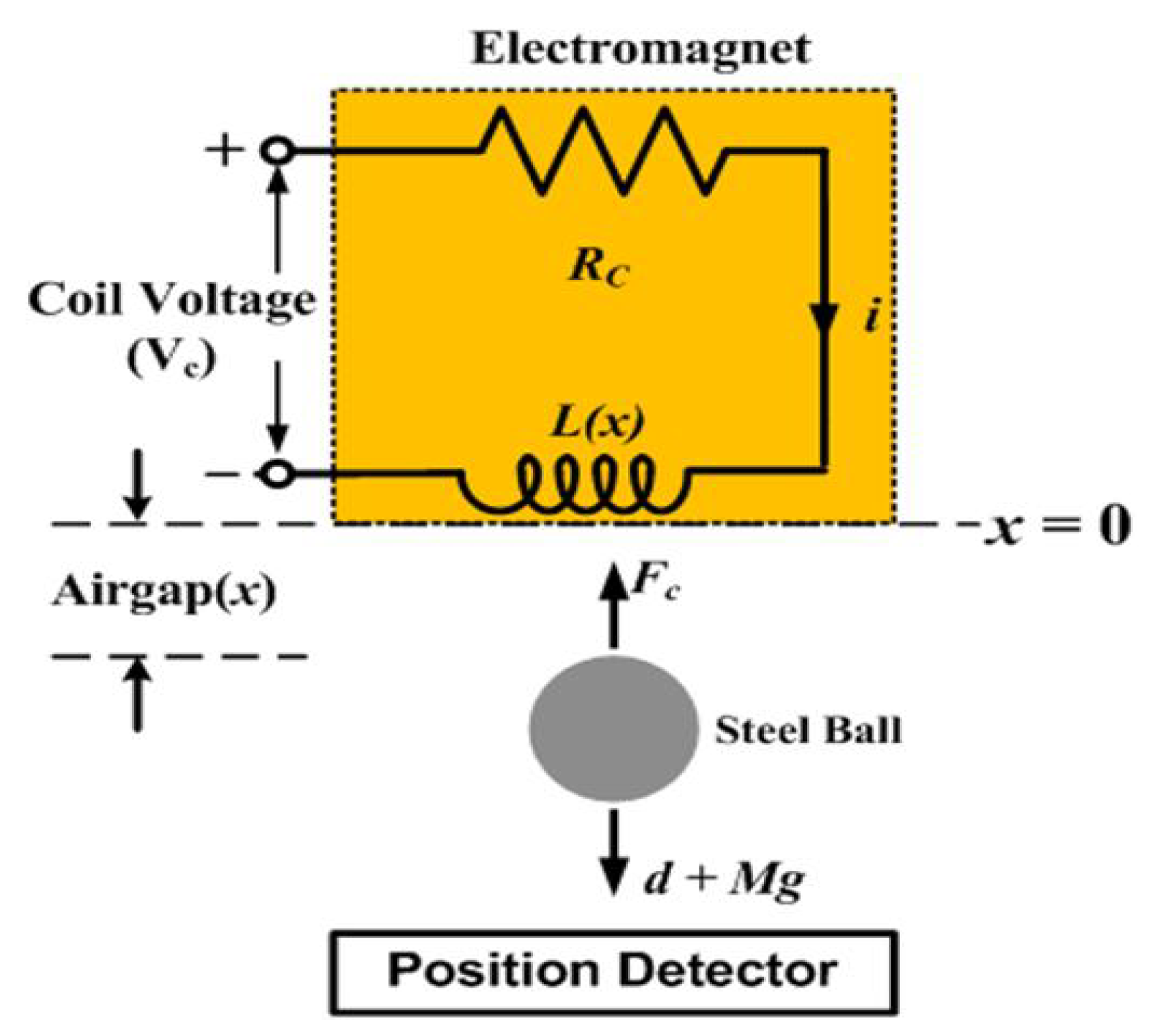
Figure 2.
DESO based estimation of sinusoidal payload disturbance () and it’s first-order derivative ().
Figure 2.
DESO based estimation of sinusoidal payload disturbance () and it’s first-order derivative ().
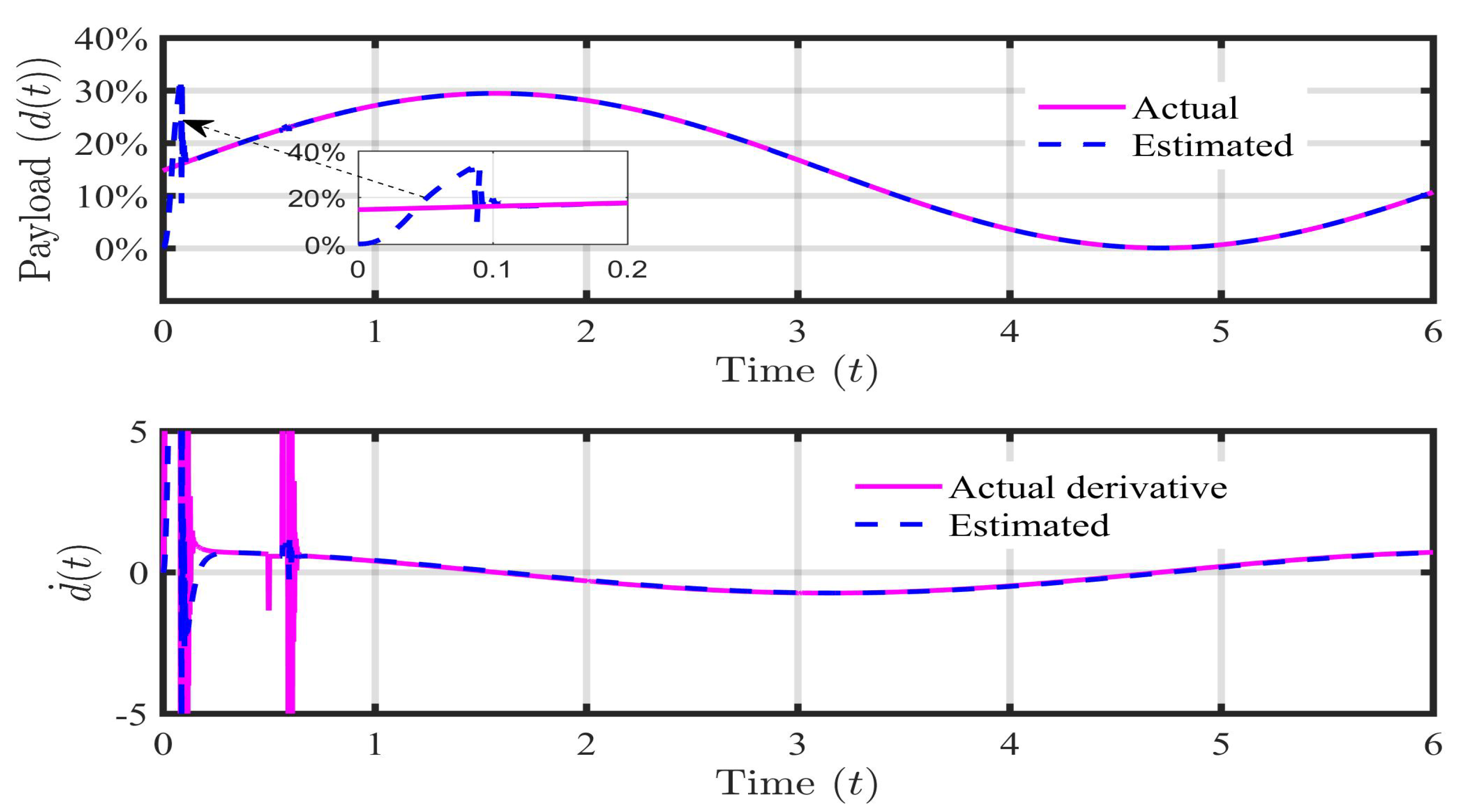
Figure 3.
Response of steel ball position () in presence of payload disturbance ().
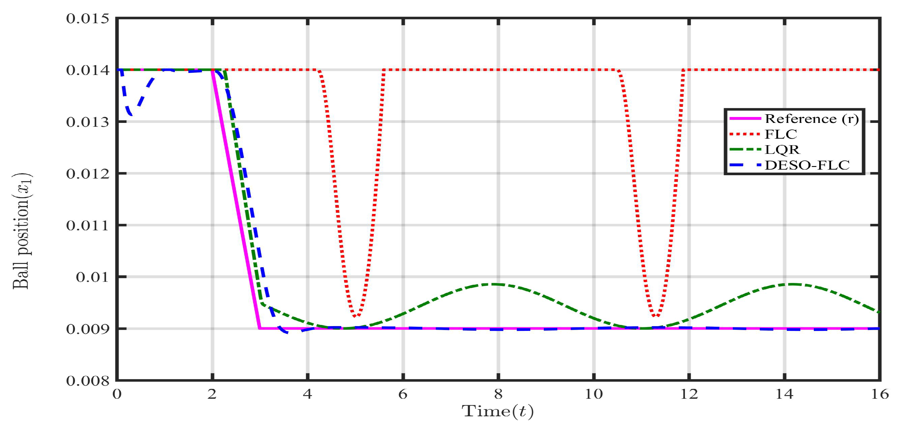
Figure 4.
Response of steel ball velocity () in presence of payload disturbance ().
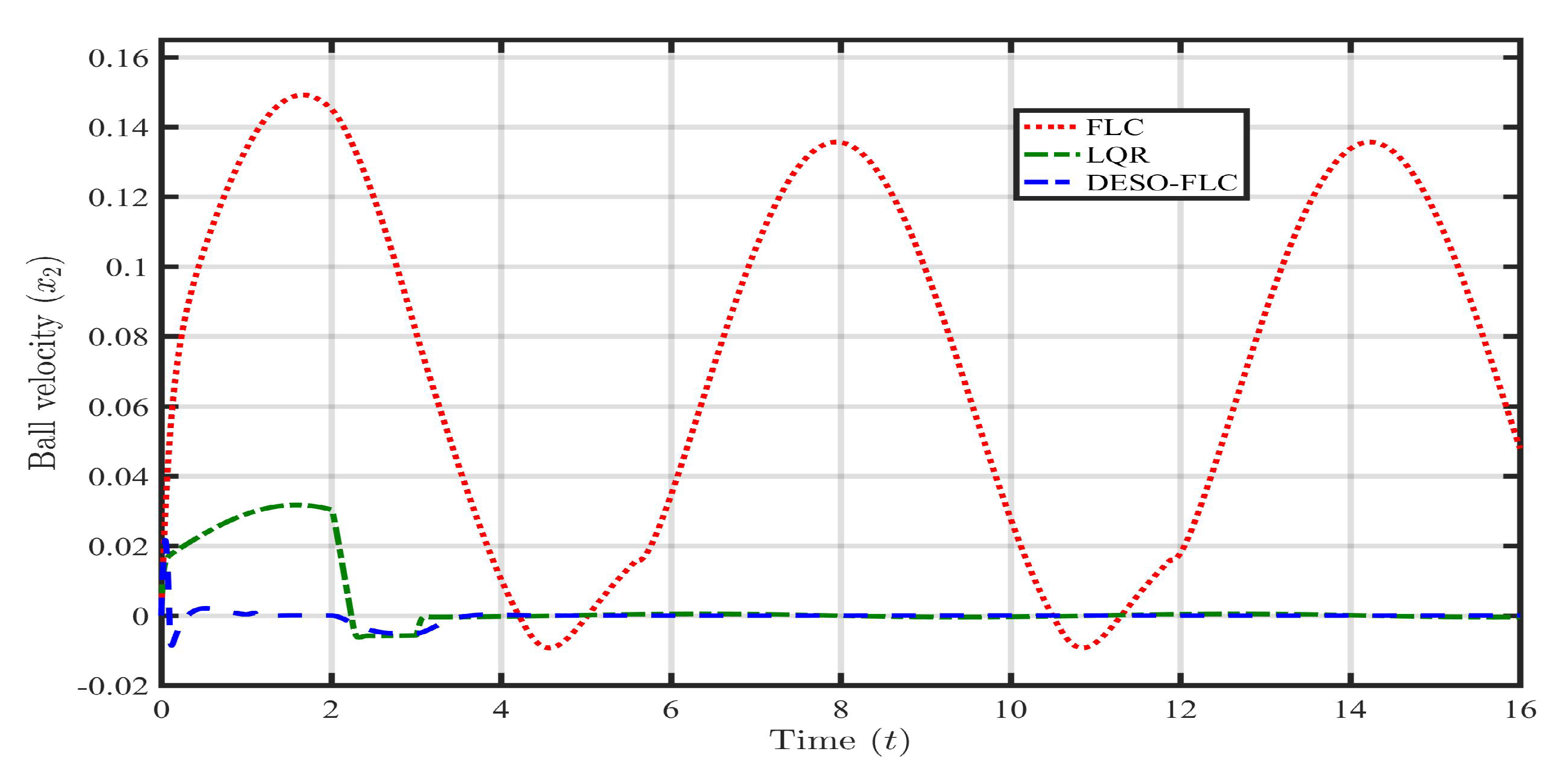
Figure 5.
Response of coil current () in presence of payload disturbance ().
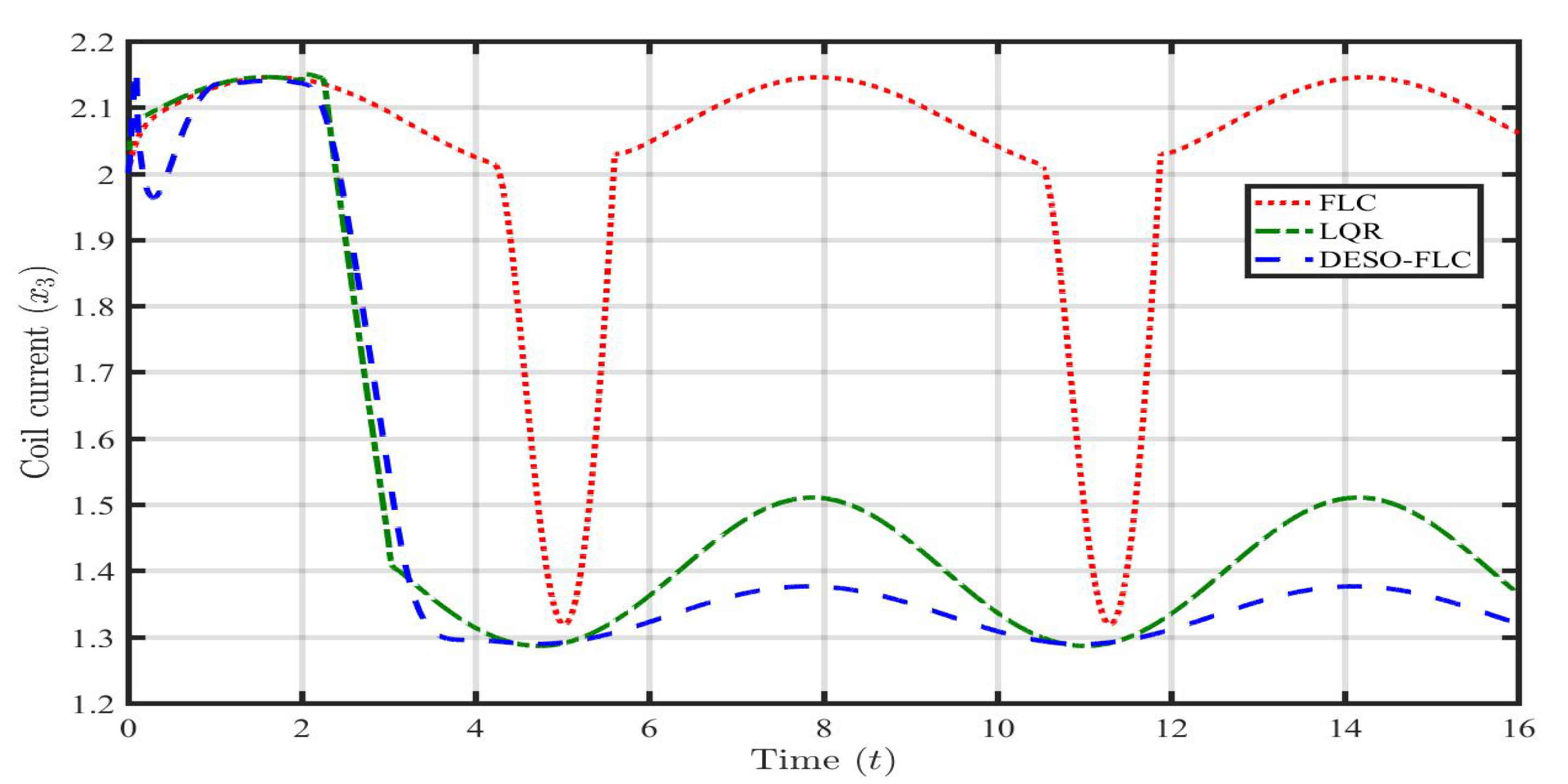
Figure 6.
Response of controlled voltage () in presence of payload disturbance ().
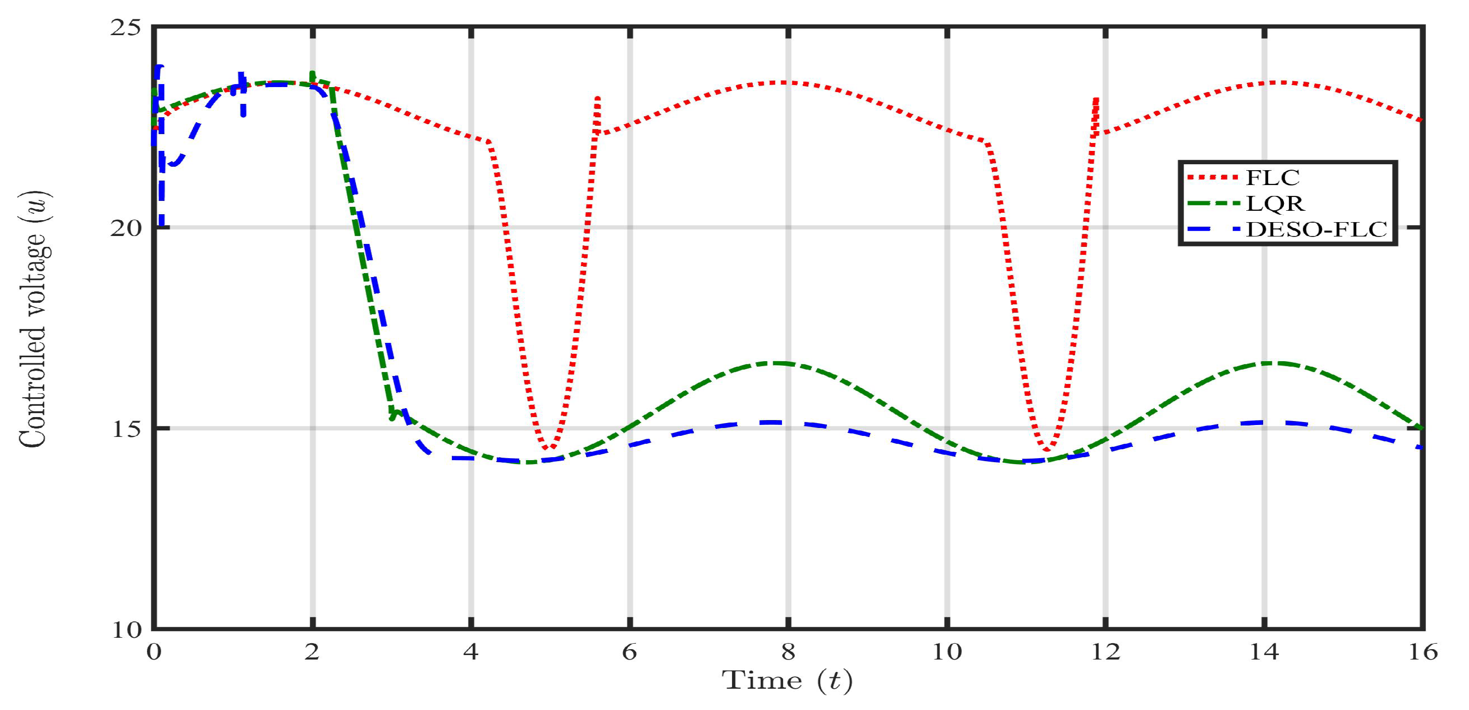
Figure 7.
DESO based estimation of disturbance due to parametric uncertainties and its first-order derivative.
Figure 7.
DESO based estimation of disturbance due to parametric uncertainties and its first-order derivative.
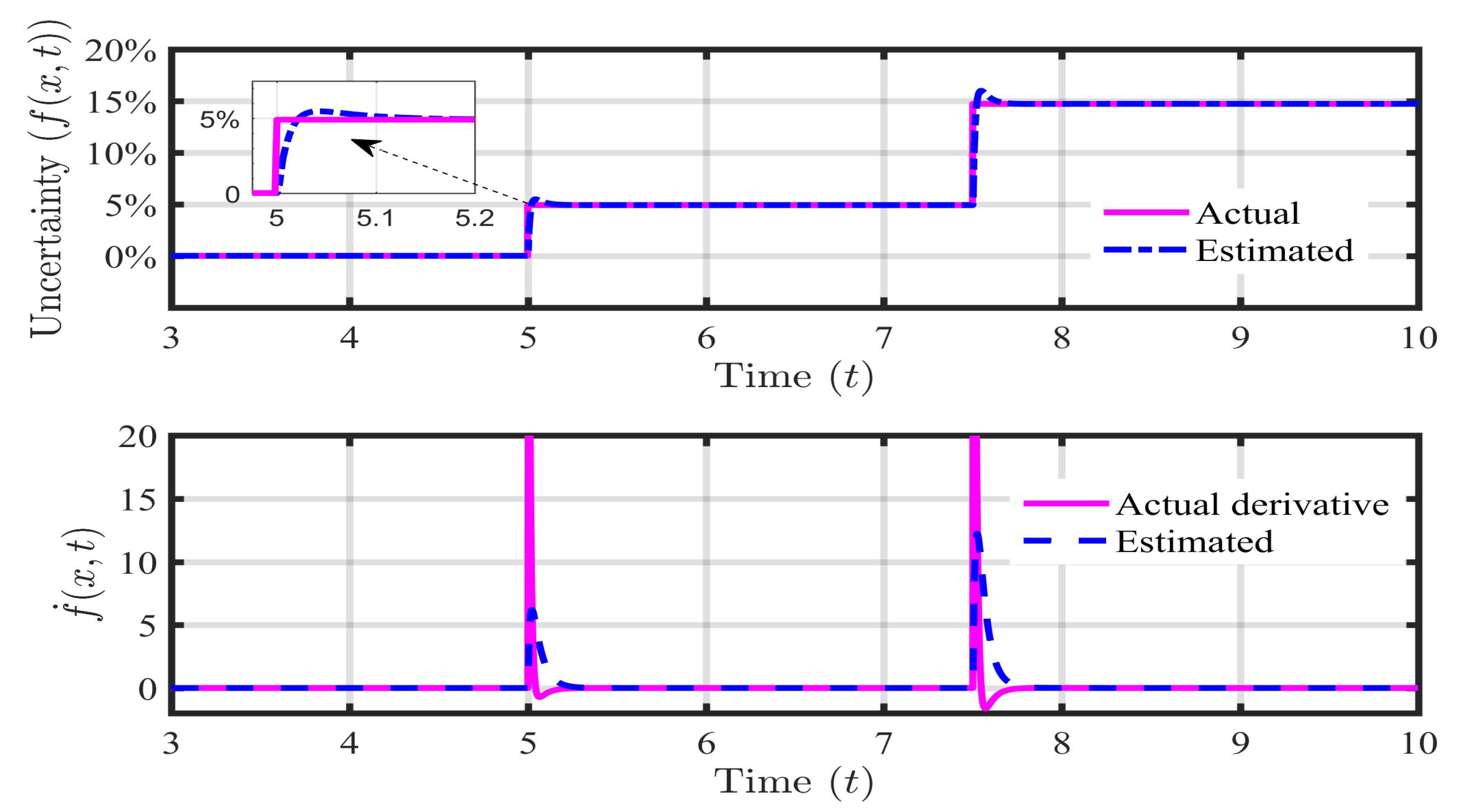
Figure 8.
Response of steel ball position () in presence of parametric uncertainties.
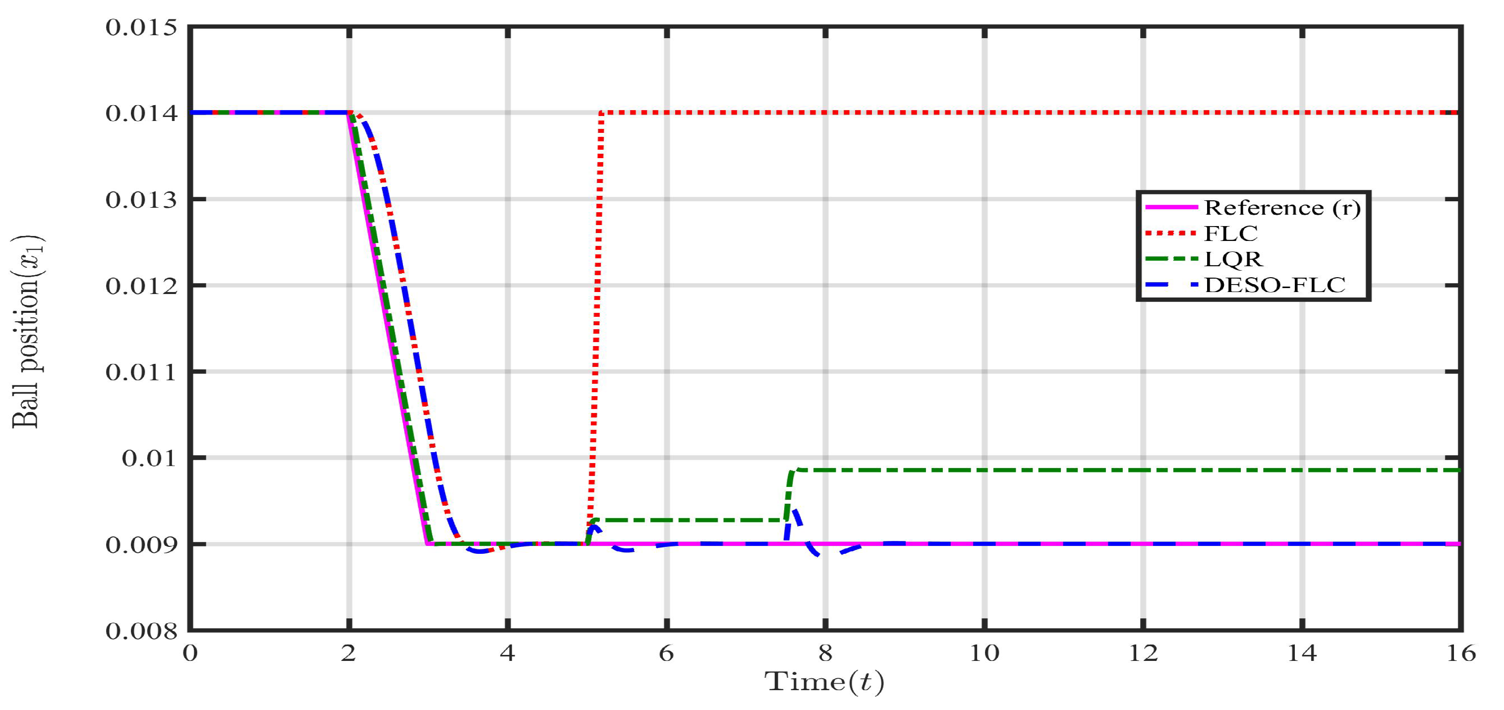
Figure 9.
Response of steel ball velocity () in presence of parametric uncertainties.
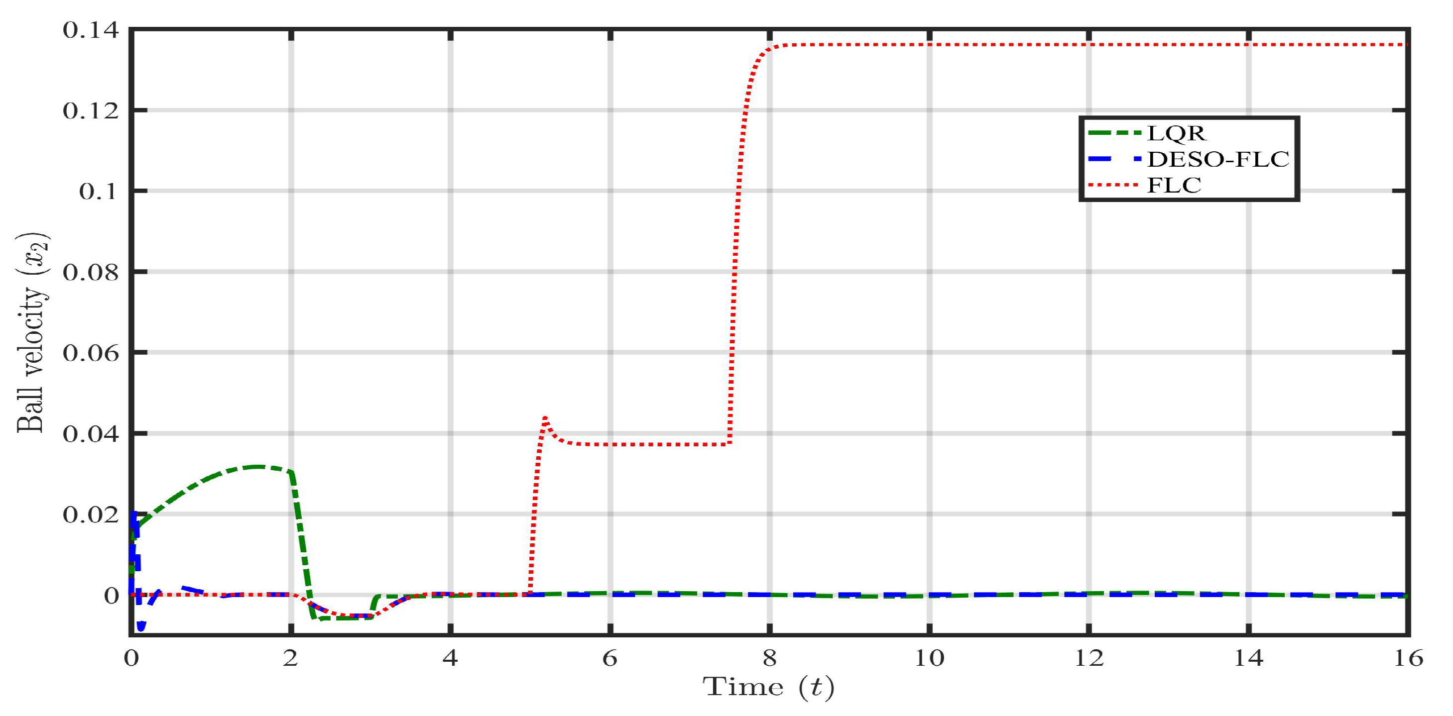
Figure 10.
Response of coil current () in presence of parametric uncertainties.
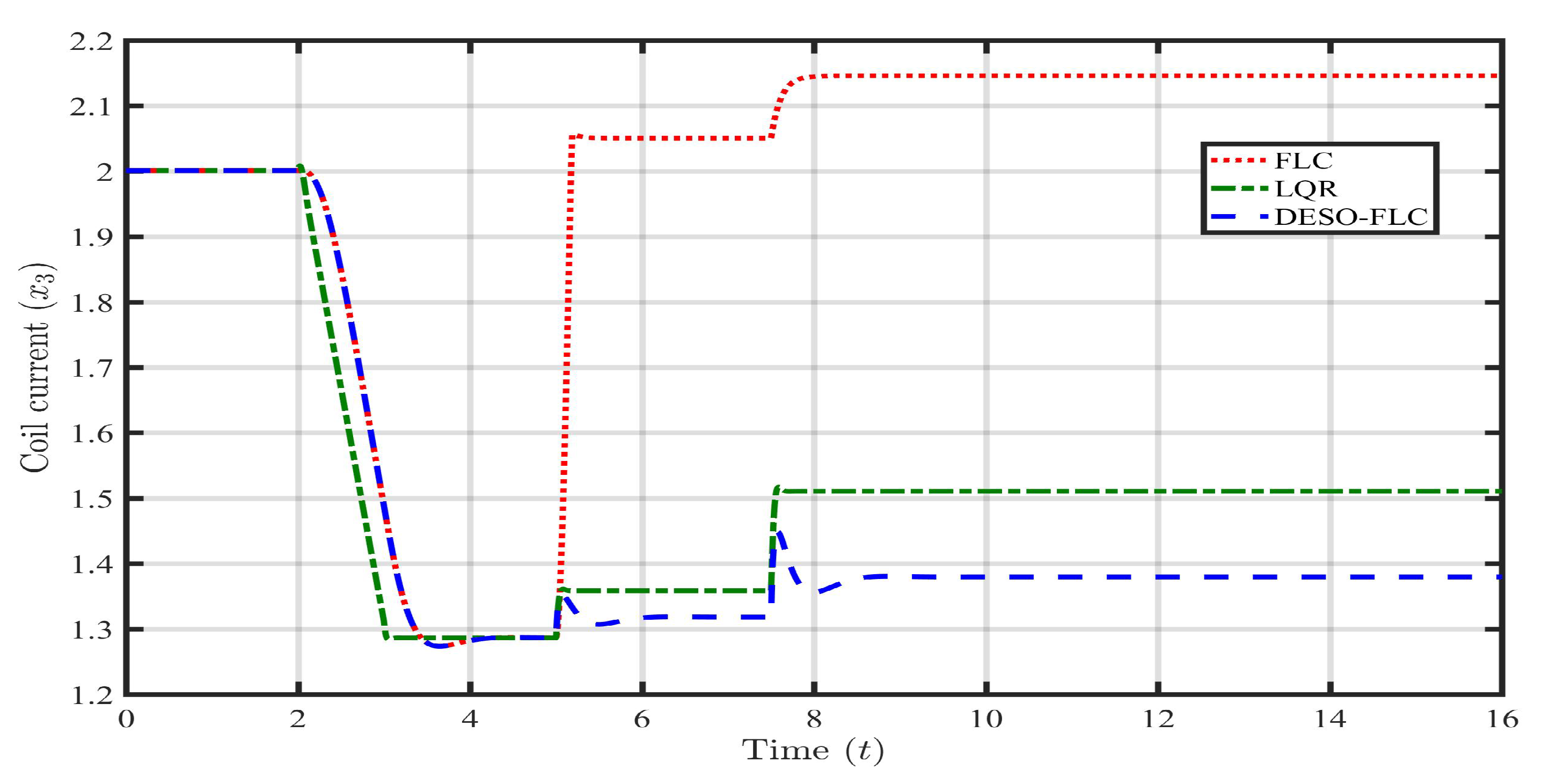
Figure 11.
Response of controlled voltage () in presence of parametric uncertainties.
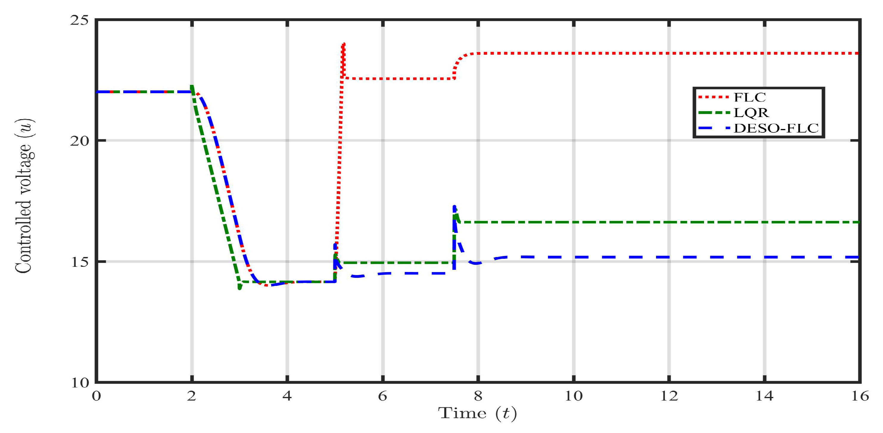
Figure 12.
DESO based estimation of mismatched lumped disturbance and its first-order derivative.
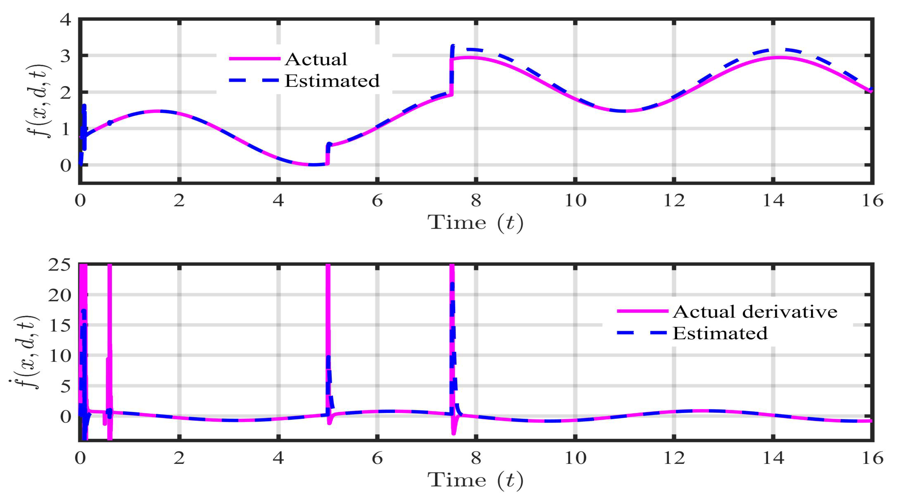
Figure 15.
Response of coil current () in presence of payload disturbance and parametric uncertainties.
Figure 15.
Response of coil current () in presence of payload disturbance and parametric uncertainties.
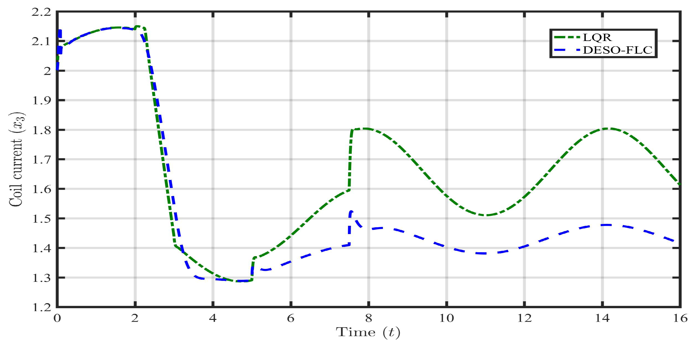
Figure 16.
Response of controlled voltage () in presence of payload disturbance and parametric uncertainties.
Figure 16.
Response of controlled voltage () in presence of payload disturbance and parametric uncertainties.
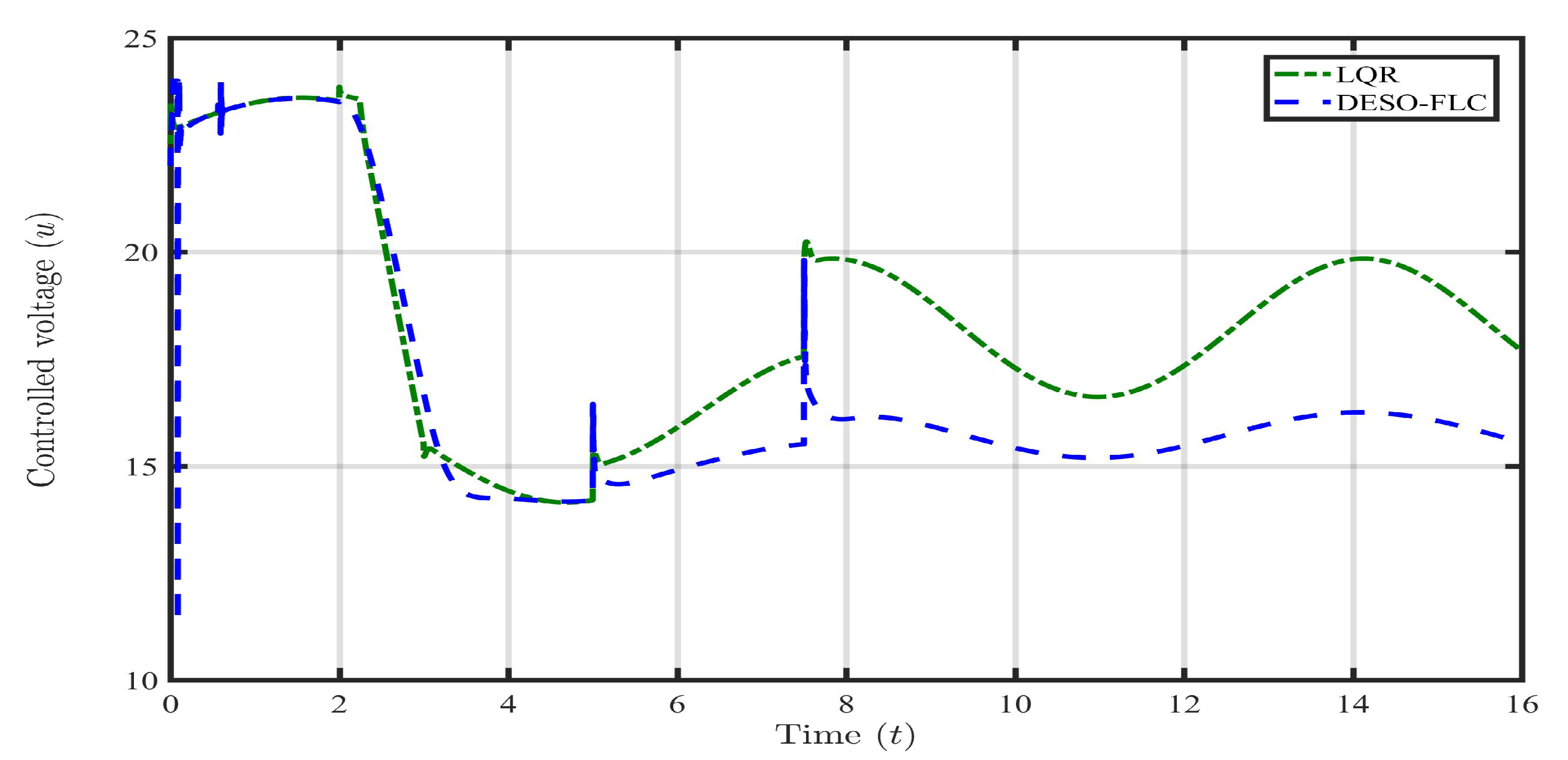

Table 1.
Simulation parameters of MLS.
| Parameter | Description | Value |
|---|---|---|
| g | gravitational constant | 9.81 |
| electromagnetic constant | 6.5308 | |
| mass of steel ball | ||
| current sensor resistance | 1 | |
| coil resistance | 10 | |
| coil inductance | 0.4125 H |
Table 2.
Comparison of ISE and ITAE using various control approaches for case 1.
| Control approach | ISE | ITAE |
|---|---|---|
| FLC | 3.608 | 0.8538 |
| LQR | 4.902 | 0.07994 |
| DESO-FLC | 1.991 | 0.006622 |
Table 3.
Comparison of ISE and ITAE using various control approaches for case 2.
| Control approach | ISE | ITAE |
|---|---|---|
| FLC | 3.733 | 0.9386 |
| LQR | 9.345 | 0.1516 |
| DESO-FLC | 1.814 | 0.005375 |
Table 4.
Comparison of ISE and ITAE using various control approaches for case 3.
| Title 1 | Title 2 | Title 3 |
|---|---|---|
| FLC | 4.178 | 0.9725 |
| LQR | 2.887 | 0.2527 |
| DESO-FLC | 1.773 | 0.005928 |
Disclaimer/Publisher’s Note: The statements, opinions and data contained in all publications are solely those of the individual author(s) and contributor(s) and not of MDPI and/or the editor(s). MDPI and/or the editor(s) disclaim responsibility for any injury to people or property resulting from any ideas, methods, instructions or products referred to in the content. |
© 2023 by the authors. Licensee MDPI, Basel, Switzerland. This article is an open access article distributed under the terms and conditions of the Creative Commons Attribution (CC BY) license (http://creativecommons.org/licenses/by/4.0/).
Copyright: This open access article is published under a Creative Commons CC BY 4.0 license, which permit the free download, distribution, and reuse, provided that the author and preprint are cited in any reuse.


