Preprint
Article

High Accuracy Detection Technique for Information Data Under the Influence of Multiple Factors based on Fractional Partial Differential Equations

Altmetrics

Downloads

165

Views

60

Comments

0

A peer-reviewed article of this preprint also exists.

This version is not peer-reviewed

Submitted:

19 February 2023

Posted:

21 February 2023

You are already at the latest version

Alerts
Abstract
In engineering practice, various types of information data are affected by many factors during the collection process. For example, information data measurement errors are caused by equipment performance and the working environment. During the transmission of detection information, the signal distortion caused by energy loss and signal interference causes unpredictable detection errors in the collected information data. Through the study of fractional calculus theory, it was found that it is suitable for studying nonlinear, non-causal, and non-stationary signals, and has the dual functions of improving detection information and enhancing signal strength. Therefore, under the influence of many factors, we applied the fractional difference algorithm to the field of information data processing. Multi-sensor detection data fusion algorithm based on the fractional partial differential equation was adopted to establish its online detection data. A multi-sensor detection data fusion algorithm based on a fractional partial differential equation is established, which effectively fuses the information data detection errors caused by various influencing factors and greatly improves the detection accuracy of information data. The effectiveness of this method is proved through its application in an experiment.
Keywords: 
Subject: Computer Science and Mathematics  -   Applied Mathematics

1. Introduction

Information detection technology have been considered as an important factor to ensure the normal operation of the control system, and the detection accuracy of multi-sensor information data is directly related to the working reliability of information detection system. Online detection technology is a multi-sensor technology, it’s the core technology of information detection systems, and the collection of real-time and accurate production information is directly related to the reliability of manufacturing systems. With the development of Internet of Things (IoT) technology, using Internet of things to collect multi-sensor detection information data in real time has become the development trend of information detection system. However, in the online detection process of the information data of the detection object, the information is affected by various factors inevitably, such as measuring instrument performance, environmental interference, and the information transmission distance, which directly affects the reliability of the information detection system. Therefore, the research on high-precision detection of information data in complex environments is of great significance to promote the development of detection technology. From the current research results, they can be divided into two categories: hardware method and software method.
The essence of hardware method is to improve the detection accuracy of information data by using high-performance detection instruments. The main research results for hardware methods are as follows. Hu Mingsong et al. [1] proposed a high-precision safety valve test architecture with three testing channels, and solve the problems of current safety valve testing effectively. Yue Huijun et al. [2] developed comprehensive sliding-separation test platform of RV reducers, realized high precision and high display test performance of various parameters of RV reducer. Reference [3,4] proposed load differential radiation pulse on the transient electromagnetic high-performance radiation source for pulse scanning detection to solve the problems of urban electromagnetic interference and insufficient harmonic components emitted by radiation sources. Reference [5,6,7] designed hardware system based on radar, and realized the real-time detection function of underground space related information by enlarging the detection information. Wang Jiaqi et al. [8] posed a one-stage remote sensing image object detection model: a multi-feature information complementary detector (MFICDet), which can improve the ability of the model to recognize long-distance dependent information and establish spatial location relationships between features.
However, in the engineering application, we found that the hardware method has the following shortcomings:
The detection accuracy of the information data depends on the performance of the detection equipment. With the improvement of the detection accuracy, the cost of the detection system is higher. Therefore, they have a low cost performance.
Their essence is to reduce the signal distortion caused by energy loss and signal interference in the information transmission process by improving the signal strength. However, when collecting information data, due to the differences in equipment performance and working environment, they cannot eliminate the measurement error of information data.
In order to solve the shortage of hardware method in information data detection under complex environment, in recent years, most researchers try to use software methods to achieve high-precision information data detection technology. The essence of software method is information data fusion algorithm. up to now, there have been many research results Common mathematical algorithms are fuzzy set theory [9], fuzzy neural networks [10], probability model [11] and particle swarm optimization algorithm [12], et al. and obtained a regrettable research review. For example, Li Huo et al. [13] proposed an integral infinite log-ratio algorithm (IILRA) and an integral infinity log-ratio algorithm based on the signal-to-noise ratio (BSNR-IILRA) to Improve the detection accuracy of laser communication detection position in the atmosphere. Shen Zhiyuan et al. [14] proposed a normalized-variance-detection method based on compression sensing measurements of received signal, and solved the problem of fast and accurate spectrum sensing technology under the condition of low signal-to-noise ratio. Jun Liu et al. [15] proposed a target detection algorithm based on the improved RetinaNet which is suitable for transmission lines defect detection, improved the intelligent detection accuracy of UAV in power system. Ru Chengyin et al. [16] proposed a lightweight ECA-YOLOX-Tiny model by embedding the efficient channel attention (ECA) module into the lightweight YOLOX-Tiny model, which has a higher respons rate for decision areas and some special backgrounds, such as the overlapping small target insulators, the insulators obscured by tower poles, or the insulators with high-similarity backgrounds. Liu Wenqiang et al. [17] introduced a point cloud segmentation and recognition method based on three-dimensional convolutional neural networks (3-D CNNs) to determine the different components of the catenary cantilever devices. Lu Yin et al. [18] proposed a complementary symmetric geometry-free (CSGF) method is, which makes the detection of cycle slips more comprehensive and accurate. Shao Lingfeng et al. [19] established the junction temperature model is based on the multiple linear stepwise regression algorithm, and used it to extract high-precision intersection online temperature. However, through the analysis of various current software methods, the following deficiencies are found in the detection of information data in complex environments.
1) They do not have the function of improving the detection information strength and cannot solve the problem of energy loss and signal interference during the transmission of information. Therefore, it is difficult to apply to engineering practice.
2) They did not analyze the cause of information data detection error, the change rule of each influencing factor and its influence on the detection value. Therefore, it is difficult to improve the detection accuracy of information data by reducing the detection error caused by various influencing factors.
Therefore, up to now, we have not found an ideal high-precision detection method for information data under the joint action of multiple influencing factors. In order to solve these problems, our team has been using the method of fractional calculus theory in data processing for many years [22,23,24,25,26,27,28] and found that fractional differential operators are suitable for studying nonlinear, non-causal and non-stationary signals, and have dual functions of improving detection information and enhancing signal strength. Therefore, by fusing the differences between information and data, it can eliminate the information and data detection errors caused by various influencing factors. By improving the signal strength of information, it can compensate the energy loss of the signal in the transmission process and improve the anti-interference ability of the signal. On the basis of previous research, this study extends the fractional differential operator in one-dimensional space to the fractional partial differential field in multidimensional space, so as to realize the high-precision detection function of information data under the joint action of multiple influencing factors.

2. Theoretical guidance and analysis

At present, many experts and scholars' research on fractional calculus theory is limited to the field of equation solving and information processing. However, how to apply it to the fusion of engineering information data and explore its application characteristics in data processing has not yet found relevant research literature.

2.1. Fractional differential

2.1.1. Fractional differential definition

Fractional differentials, also named fractional derivatives, it extend the differential order of an integer-order differential equation to a fractional order. The concept of the fractional differential emerged in 1812 [8]. After hundreds of years of research, fractional differentials does not have a unified definition, many scholars have proposed their own definition methods and theoretical systems based on their own understanding and application fields. At present, the commonly used definitions are those of Grunwald–Letnikov (G-L), Caputo, and Riemann–Liouville (R-L) [9,10].
Among the three definitions, Because the G-L definition has the advantage of fast calculation speed, it is widely used in engineering field, therefore, this paper uses G-L definition to study the application technology of fractional calculus theory in detection information data fusion.
Suppose there is a real number v, its part of v is denoted as [v], if the function f ( t ) has (n + 1)-order continuous derivatives within the interval [a , t], when v > 0 and n ≥ [v], the G-L definition of fractional v-order derivative as
D t v a f ( t ) = lim h 0 f h ( v ) ( t ) = lim h 0 h v j = 0 [ t a h ] ( 1 ) j [ v j ] f ( t j h )
In the equation above, 0 ≤ n-1 < n, ( v j ) is a binomial coefficient, and its formula is
[ v j ] = v ( v 1 ) ( v 2 ) ( v j + 1 ) j !
In Eq. (2), when h 0 , then n ; let h = ( t a ) / n , then n = [ ( t a ) / h ] .

2.1.2. Effect of fractional differential on detection signal

For years, many mathematicians and scientists have tried to apply fractional calculus theory in signal processing and have achieved good application effects [11,12]. It is assumed that there is a detection signal S ( t ) , where S ( t ) L 2 ( R ) , and its Fourier transform is
S ( ω ^ ) = R S ( t ) e i ω t d t
Let S v ( t ) be the v-order differential of S ( t ) . According to the properties of the Fourier transform, we know the v-order differential operator is equal to the multiplicative operator of the v-order differential multiplier function d ^ ( ω ) = ( i ω ) v . Thus, we can obtain the following equation:
D v S ( t ) F T ( D ^ S ) v ( ω ) = ( i ω ) v S ( ω ^ ) = | ω | v e i θ v ( ω ) S ( ω ^ )
From the perspective of signal modulation, the physical meaning of the fractional differential of a detection signal is equivalent to the generalized amplitude and phase modulation. From the perspective of signal processing, the v-order fractional calculus operation of the detected signal is equivalent to establishing a linear time invariant filtering system for the signal, and its filtering function is
d v ( ω ^ ) = [ ω ] v e i θ v ( ω )
From Eq. (5), we can drawing the spectrum characteristic curve of the fractional differential operator, as shown in Figure 1:
According to Figure 1, we can see that fractional differential operators have the following characteristics in information processing.
(1) In the processing of detection signal, fractional differential operator can enhance the medium and high frequency part of the signal. The lifting amplitude increases nonlinearly and rapidly with the increase of frequency and fractional differential order, so it has the function of enhancing signal strength. However, with the increase of frequency, the gap between the signal enhancement values of fractional differential operators under different orders tends to narrow gradually.
(2) When ω > 1, with an increase in the fractional order v and signal frequency ω, the variability between the signal enhancement coefficients of the fractional-order differential operators at different orders tends to decrease, and with an increase in frequency, the enhancement effect of the differential operators of the same order on the signal intensity at different frequencies is basically the same.

2.2. Fractional partial differential

From the analysis of the amplitude frequency characteristics of fractional differential operators, we can know that in the signal enhancement stage, when the influencing factors reach a certain value, the fractional differential operator can fuse the differences between the detection data caused by the influencing factor effectively, so, the fractional calculus is used to describe many phenomena in engineering and science [13,14]. The fractional differential equations have been used enormously for last two decades because of their varied applications in many spheres of physical and biological sciences [15,16,17], but it can only be applied to processing one-dimensional signal. In the process of information data collection, the detection information will be affected by many factors, such as testing equipment performance, equipment working environment, et al. Therefore, we need to apply the fractional partial differential equations to expand the fractional differential operators in multi-dimensional space.

2.2.1. Fractional partial differential equation

In order to simplify the calculation workload, it is assumed that the information data value is affected by two factors. According to the G-L definition of the fractional partial differential, we extend the fractional differential operators to two-dimensional space. Assuming that the information acquisition system collects any given two-dimensional energy signal S ( x , y ) , and S ( x , y ) L 2 ( R ) , we can obtain the fractional partial differential equation S v ( x , y ) of the signal as
S v ( x , y ) = v S ( x , y ) x v + v S ( x , y ) y v
Refer to equation (1), Can be obtained the following formula
{ v S ( x , y ) x v lim h 1 0 h 1 v i = 0 n ( 1 ) i ( v i ) S ( x i h 1 ) v S ( x , y ) y v lim h 2 0 h 2 v j = 0 m ( 1 ) j ( v j ) S ( x j h 2 )

2.2.2. Applications of the fractional partial differential equations

Compared with an integer order partial differential equation, the outstanding advantage of fractional partial differential equation is that it can better simulate the physical process and dynamic system process of nature. Compared with fractional differential equations, a fractional partial differential equation can take the unknown quantity in the equation as the influence factor to realize the fractional differential treatment of multiple influence factors in the equation. Because fractional partial differential equations have the above advantages, in recent years, the research on the characteristics and applications of fractional partial differential equations has become the focus of many experts and scholars. Some research results have been widely used in the research of technical problems in the fields of temperature field distribution, image processing, mechanical analysis, and detection technology [18,19,20,21,22]. For example, WANG Bao et al [23] applied fractional partial differentials to achieve the research goal of thickness design of high-temperature protective clothing under actual limited conditions; ZHOU Shangbo et al [24] applied them to prove their advantages in image denoising and reducing step effect and in denoising and super-resolution reconstruction. SHEN Tianlong [25] applied fractional partial differentials in the research field of fluid mechanics; ZUO Yanhong et al [26,27,28,29,30,31,32] applied it in test data fusion processing technology of a discrete manufacturing system.

3. Online detection data fusion algorithm based on fractional differentiaL

3.1. Fusion algorithm model based on fractional partial differential equations

IOT is used to collect a group of production information Si (i = 1, 2,... n) of the same type, due to the influence of test instrument performance, working environment and information transmission distance et al, it leads to great differences between the data collected by information systems. Therefore, we need to establish relevant information and data fusion models to effectively remove the detection errors caused by the above factors and improve the detection accuracy of information.
We assume that the monitoring information of mobile equipment collected by wireless network technology is mainly affected by factors x and y, and the functional relationship between the signal detection value and the influence factor is J(x,y). Because the influences of the two influence factors x and y on the detected value are independent of each other, the calculation method of the function for influence factors x and y are interdependent. According to the spatial function B V v ( Ω ) of differential detection data fusion, the model of mobile equipment monitoring information data fusion algorithm based on fractional partial differential equation under the IoT is as follows:
J t = [ i = 0 n D x v J ( x + i h 1 , y ) | D v J | . D x v ( i h 1 ) + j = 0 m D y v J ( x , y + j h 2 ) | D v J | . D y v ( j h 2 ) ] + λ ( J 0 J )
In the above equation,
{ D x v J ( x , y ) J ( x , y ) + ( v ) J ( x h 1 , y ) + ( v ) ( 1 v ) 2 J ( x 2 h 1 , y ) + + Γ ( n v ) Γ ( n + 1 ) Γ ( v ) J ( x n h 1 , y ) D y v J ( x , y ) J ( x , y ) + ( v ) J ( x , y h 2 ) + ( v ) ( 1 v ) 2 J ( x , y 2 h 2 ) + + Γ ( m v ) Γ ( m + 1 ) Γ ( v ) J ( x , y m h 2 )

3.2. Fusion process based on fractional partial differentials

In order to obtain the information data of the detection object in real time and effectively, the information detection system often uses the Internet of things to collect all kinds of information data. Based on the integration idea under the distributed system, classify the collected data, obtain the required information data firstly, then analyze the main factors leading to the difference between the data, and fuse the differential information data by using the detection data fusion model based on fractional partial differential equation, so as to reduce the difference of detection data between sensors effectively. In the multi-sensor detection data fusion algorithm model based on the fractional partial differential equations, the premise of data fusion is to obtain the function S(x,y) for a data detected value S and influence factor x and factor y. A fusion model of different detection data can be obtained by fractional partial differential calculations. The fusion process of the detection data is as follows:
(1) Apply the Internet of things to obtain all kinds of detection information in real time, and select the required experimental data by analyzing the detection data..
(2) Analyzing the characteristics of information data, find the main factors x and y which affecting the measured value of data.
(3) Through the fitting method, determine the functional relationship S(x,y) between the detected value of information data S and its influencing factor x and y preliminarily.
(4) Apply the fractional partial differential equation to fuse the information data S, obtain the fused information data Sv.
(5) Analyze the fused information data, evaluate the application effect of fractional calculus theory in information data fusion..
(6) End.

4. Application of algorithm in the information data detection system

4.1. Problem description

To compare the performances of the data fusion algorithm, we selected the experimental data in literature [33]. The measured temperature data of a thermostat was collected by 8 smart temperature sensors, and the data is measured every hours for a total of eight times, then apply the Internet of things sent the detected data to the information collection system. The measured values of each sensor are shown in Table 1. Take the average value of the measured values as the real value, that is 53.07 ℃. From the data shown in Table 1, it can be seen that the data 46.52, 47.35, 48.43, 56.05, 57.66 and 58.34 in the table are exceed the international standard of common deviation obviously, so they should be removed before fusion. From Table 1, we can see that the total measurement error of 8 sensors at different time points T=1.58, the standard deviation of the detected data between sensors Sx=0.251, and the standard deviation of different times of measurement data Sy = 0.333.

4.2. Analysis and processing of test data

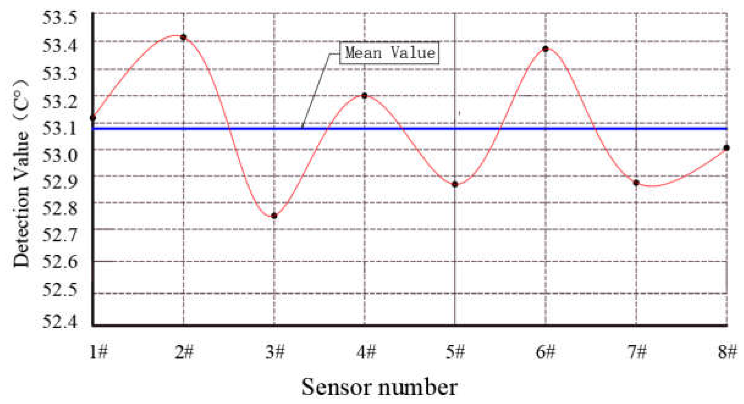
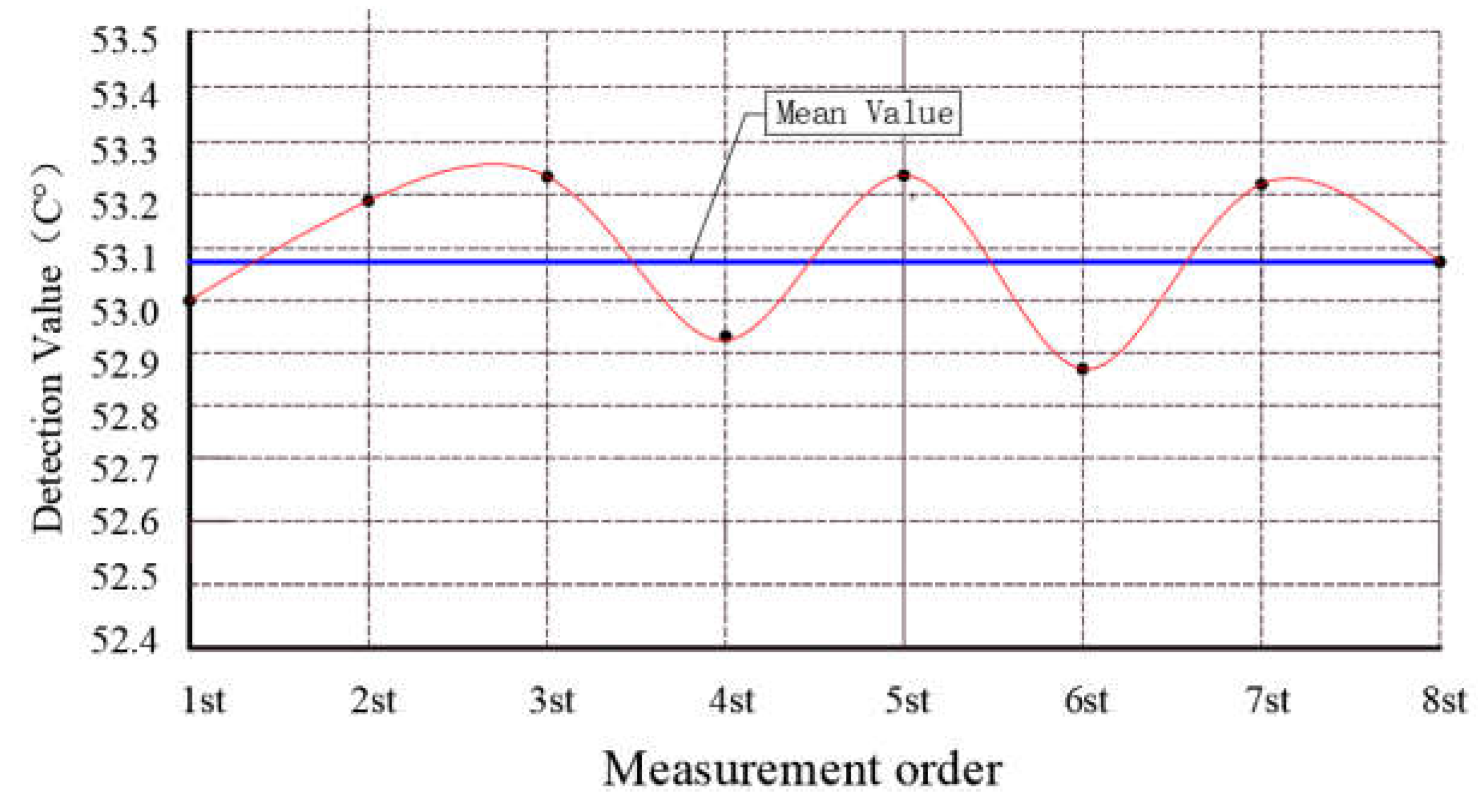
Using the data shown in Table 1, take the measured average value of each sensor as its measured value Fi, and draw the distribution curve of the measured data of each sensor, as shown in Figure 2. The average value of the detected values of the eight sensors at different time points is the measured true value Fj, and its data distribution curve is drawn, as shown in Figure 3. It is found that their measured values present an irregular discrete distribution above and below the mean value of 53.07 °C.
According to the experimental data given in Table 1 and the data distribution curves shown in Figure 2 and Figure 3, we find that the measured values have the following characteristics:
(1) In the measurement of thermostat temperature, due to the difference in the performance of detection instruments, there is a big difference between the same detection information data, which indicates that the performance of detection equipment and instruments is an important factor affecting the temperature measurement value.
(2) When measuring at different times, due to the difference of the detection environment, there is a large difference between the measured values of the same information data at different time points. Therefore, the detection environment is also an important factor affecting the measured value.

4.3. Fitting of functional relationship between detected value and influence factor

According to the common sense of surveying, standard deviation is the best performance index to measure the accuracy of information data; so, in this case, we use the performance of the test equipment as the influencing factor x and the working environment of the equipment as the influencing factor y to deal with the test value of the thermostat temperature effectively, and using the sandard deviation Sx and Sy as the influencing factors to establish the functional formula between them and the measured value Si. Because the least square method has the advantage of doesn't need a priori information about the data in the process of data processing, because it can obtain ideal data fusion accuracy; so, it is used to fit the measurement data through function polynomials widely. Therefore, this paper uses the least square method to fit the functional formula of S (x) and S(y) is as follows:
{ S ( x ) = a 0 + a 1 x + a 2 x 2 + + a n x n S ( y ) = b 0 + b 1 y + b 2 y 2 + + b m y m
From the data in Table 1, it can be seen that every experimental datum is equal to S (xi) and S (yj); so, S(xi) = S(yj); then, we obtain the following equation:
S ( x , y ) = ( S ( x ) + S ( y ) ) / 2 = ( a 0 + a 1 x + a 2 x 2 + + a n x n + b 0 + b 1 y + b 2 y 2 + + b m y m ) / 2

4.3.1. Order of the polynomial

When fitting a polynomial via the least squares method, the order of the polynomial should be less than the number of detected values. Thus, a higher order does not guarantee a better fusion effect, but rather, there is an optimal order value. In this case, the number of sensors used is 8, and the number of measurements is 5, so the order n of the polynomial in this case is less then 8, and m is less then 8. Therefore, We used the polyfit function in the MATLAB software to calculate the average error value of the polynomial at different orders.

4.3.2. Calculation of polynomial coefficients

(1) Functional relationship between influence factor x and detection value S
According to Eq. (10), the function S(x) is obtained by calculating the values of coefficient ai and order n. According to the basic definition of the least squares method, the order of the polynomial shown in the equation of S(x) should be less than the number of samples; so, n < 8. According to the experimental data shown in Table 1, using the polyfit function in MATLAB software, we can conclude that when the order of the polynomial n = 1, the error between the fitting value of each sensor's detection data is 1.0779—the smallest one. In this case, the functional relationship between the detection data S and the influence factor x as
S(x)= 1.711x+52.645
(2) Functional relationship between influencing factor y and detection value S
According to the above theory, the function S(y) is obtained by calculating the values of coefficient bi and of order m used in Eq. (10). According to the basic definition of the least squares method, the order of the polynomial S(y) shown in equation (10) should be less than the number of samples, so m < 8. According to the experimental data shown in Table 1 and the polyfit function in MATLAB software, we can conclude that when the order of the polynomial m = 1, the error between the fitting value of the detection data of each sensor is 0.3667 and is the smallest. In this case, the functional relationship between the detection data S and the influence factor y as
S(y)=0.667y+52.873

4.4. Detection data fusion technology based on fractional differential operator

4.4.1. Selection of fractional order v and step h

(1) Select the value of fractional order v
According to the amplitude and frequency characteristics of the fractional differential operator, we know that when the differential order is 0 < v < 1, the fractional differential operator has a nonlinear function retaining the very low frequency part of the signal and enhancing the low frequency part of the signal, and the enhancement effect becomes increasingly obvious with the reduction of the order. To save space, this case considers the fractional order v=0.5 as the middle value of the range [0,1], and studies the application effect of fractional partial differential equation in the data fusion processing of bearing oil temperature sampling under the Internet of things.
(2) Select the value of discrete step h
From Eq. (9), it can be seen that the smaller h can obtain accurate fusion data, but it has the shortcoming of a low efficiency. In this case, the fusion speed and fusion accuracy are comprehensively considered. According to the value range [0.15,0.37] of the influence factor x (sensor standard deviation) shown in Table 1, when the distance walk length h1 = 0.01, and the number of steps to be calculated n = 22; according to the value range [0.23,0.48] of the influence factor y (information energy consumption loss) shown in Table 1, when the distance walk length h2 = 0.01, and the number of steps to be calculated m = 25. In this way, the fusion calculation steps m and n of the influence factor x and the influence factor y are similar and can meet the requirements of calculation speed and accuracy at the same time.

4.4.2. Data fusion and results analysis

Next, the values of Eq. (9) and related parameters (v, h1, h2, m, n) are substituted into the mathematical model of mobile device detection data fusion processing based on the fractional partial differential equation shown in Eq. (8) and Eq. (9). We obtain the following calculation formula:
S 0.5 ( x , y ) = 0.5 S ( x , y ) x 0.5 + 0.5 S ( x , y ) y 0.5
In the above equation,
{ 0.5 S ( x , y ) x 0.5 lim h 1 0 h 1 0.5 i = 0 19 ( 1 ) i ( 0.5 i ) S ( x i h 1 ) 0.5 S ( x , y ) y 0.5 lim h 2 0 h 2 0.5 j = 0 34 ( 1 ) j ( 0.5 j ) S ( x j h 2 )
According to the above formulas, we can calculate the measured temperature data of thermostat S(xi, yj) of each temperature sensor by 0.5-order partial differential equation, and the results of 0.5-order partial differential equation fusion under the influence factor x are shown in Table 2, and the influence factor y are shown in Table 3.
Combining equations (12), (13), (14) and (15), we can get the values of 0.5-order partial differential of the measured value of each sensor at different time points, as shown in Table 4.

4.4.3. Fusion processing results of detection data by 0.5-order partial differential equation
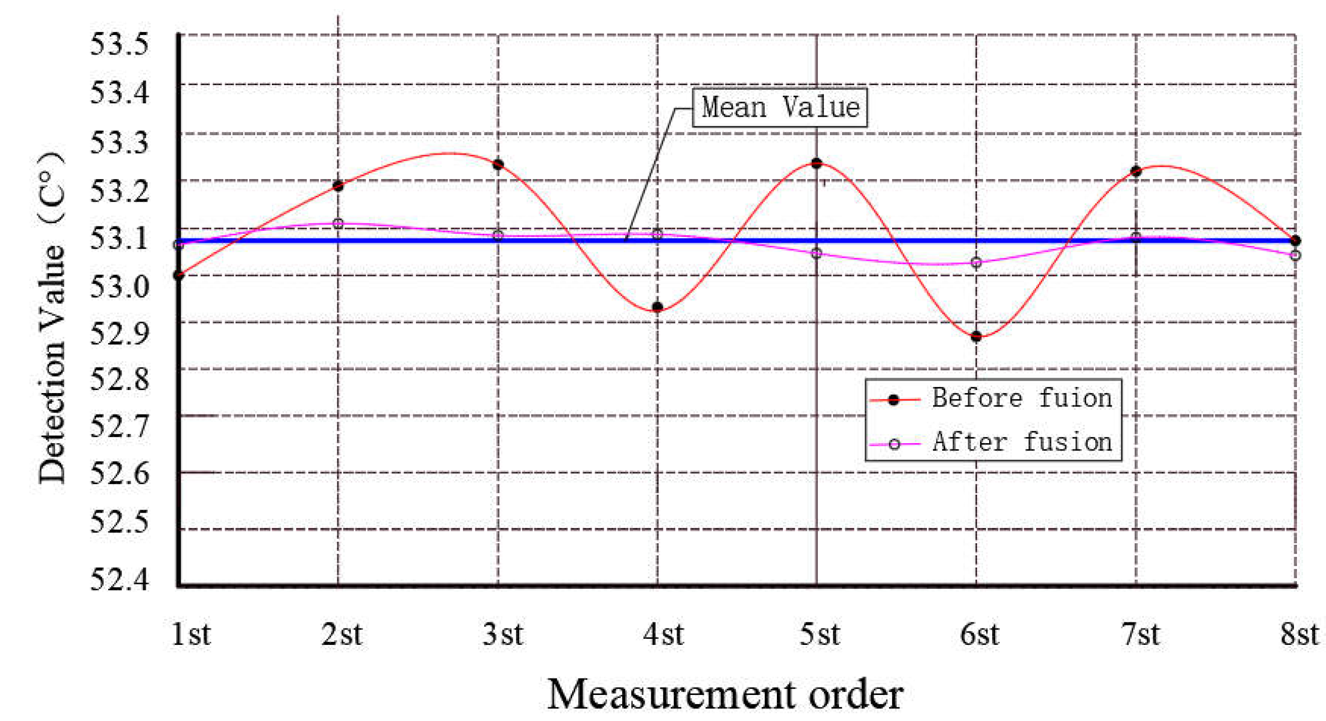
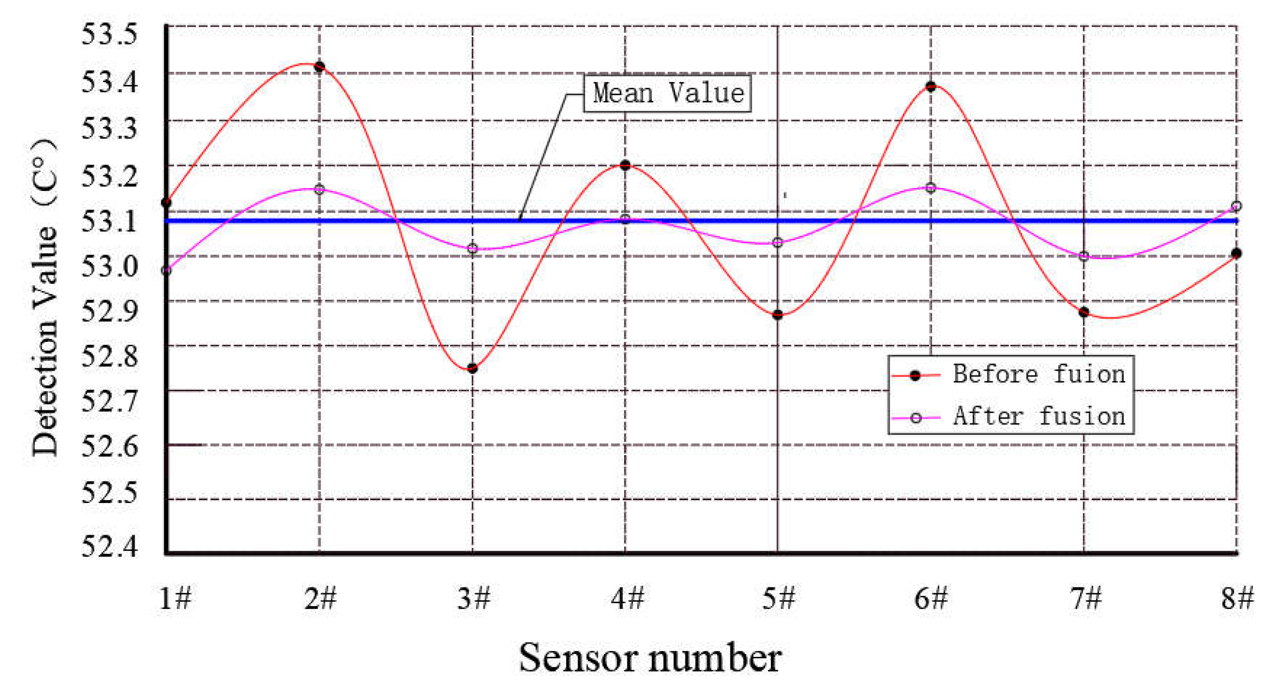
Comparing the mean value F of Table 1 with the mean value F0.5 of Table 2, we can conclude that after the 0.5-order partial differential fusion, the numerical magnification is K=1.166, it can improve the anti-interference ability of the signal and the reliability of information transmission. In order to compare the effect of data fusion with other algorithms, we divide the data in Table 4 by K and calculate the final data processing result, as shown in Table 5. From Table 5, We can see that after fused by 0.5-order partial differential equation, the fusion accuracy was improved effectively. Analysis from measurement error, The total absolute error of the methods used in this paper was 0.175, which is significantly lower than the total absolute error of 1.58 obtained by the average value algorithm, the total absolute error of 0.395 obtained by the algorithm described in Reference [27], and the total absolute error of 0.335 obtained by the algorithm described in Reference [34]. After processed by 0.5 order partial differential algorithm, the standard deviation between the measured values of each sensor and information data at different time points is about one tenth of that before processing. According to the data shown in Table 4, the comparison chart of standard deviation between the measured values of each sensor and different time points before and after being processed by the 0.5 order partial differential algorithm is drawn. It can be found that a straight line is distributed near the average value between the processed data. Experiments show that the 0.5 order partial differential algorithm has a strong fusion ability for experimental data.
Figure 3. Distribution curve of the detection data fused by 0.5-order partial differential equation.
Preprints 68857 g004
Figure 4. Distribution curve of the detection data fused by 0.5-order partial differential equation.
Preprints 68857 g005

5. Conclusion

In engineering practice, the detection information can not avoid the common influence of multiple irregular change factors, which brings unpredictable measurement errors. In this paper, we find that fractional differential operators are suitable for studying nonlinear, non causal and non-stationary signals. Therefore, the fractional differential algorithm will be applied to the processing of complex detection information. According to the number and type of influencing factors, the fractional differential operator is extended to the fractional partial differential field, which realizes the effective fusion processing of information data under the joint action of multiple influencing factors. By enhancing the strength of the detection signal, the anti-interference ability of the detection information in the transmission process is improved, and the information and data distortion caused by the energy loss is compensated. In engineering applications, we can adjust the value of the parameter fractional order v and step h in the algorithm to meet the information data detection target required by the system. The difference between information data is fused to improve the measurement accuracy of detection information. The effectiveness of this method is proved by an example.

Acknowlelgment

Project supported by the National Natural Science Foundations, China (No.51878005 and No.51778004); Anhui Provincial Education Commission Foundation, China (No.KJ2020A0488).

References

  1. Hu, M.-S. Design and development of a high-precision automatic safety valve testing system. Adv. Mech. Eng. 2020, 12. [Google Scholar] [CrossRef]
  2. Yue, H.; Wu, X.; Shi, Z.; Zhang, Y.; Ye, Y.; Zhang, L.; Fu, Y. A comprehensive cycloid pin-wheel precision reducer test platform integrated with a new dynamic measurement method of lost motion. Metrol. Meas. Syst. 2021, 29, 207–229. [Google Scholar] [CrossRef]
  3. W. Li, B. Li, C. Shu, et al. New muti-resolotion and muti-scale electromagnetic detection methods for urban underground spaces. Journal of Applied Geophysics 2018, 159, 742–753. [CrossRef]
  4. W. Li, B. Li, C. Shu, et al. Study on muti-resolotion imaging of urban underground spaces based on high performnce transient electromagnetic source. Chinese Lournal of Applied Geophysics. 2014, 63, 4553–4564.
  5. Ahmed, N.; Radchenko, A.; Pommerenke, D.; Zheng, Y.R. Design and Evaluation of Low-Cost and Energy-Efficient Magneto-Inductive Sensor Nodes for Wireless Sensor Networks. IEEE Syst. J. 2018, 13, 1135–1144. [Google Scholar] [CrossRef]
  6. Pal, A.; Kant, K. NFMI: Near Field Magnetic Induction based communication. Comput. Networks 2020, 181. [Google Scholar] [CrossRef]
  7. Guo, H.; Sun, Z.; Zhou, C. Practical Design and Implementation of Metamaterial-Enhanced Magnetic Induction Communication. IEEE Access 2017, 5, 17213–17229. [Google Scholar] [CrossRef]
  8. Wang, J.; Gong, Z.; Liu, X.; Guo, H.; Lu, J.; Yu, D.; Lin, Y. Multi-Feature Information Complementary Detector: A High-Precision Object Detection Model for Remote Sensing Images. Remote. Sens. 2022, 14, 4519. [Google Scholar] [CrossRef]
  9. Muñoz, J.; Molero-Castillo, G.; Benítez-Guerrero, E.; Bárcenas, E. Data fusion as source for the generation of useful knowledge in context-aware systems. J. Intell. Fuzzy Syst. 2018, 34, 3165–3176. [Google Scholar] [CrossRef]
  10. Hou Xin, Zhang Dongwen, Zhong Ming. Data Aggregation of Wireless Sensor Network Based on Event-Driven and Neural Network. Chinese Journal of Sensors and Actuators 2014, 27, 142–148. [Google Scholar]
  11. Hedjazi M H, Ghari M. Abolmaesumi P. Distribution of Fiducial Registration Error in Rigid-body Point-based Registration. IEEE Trans. on Medical Imaging 2009, 28, 1791–1801. [Google Scholar] [CrossRef]
  12. He r, Wang YJ, Wang Q, Zhou Jh, Hu CY. An improved particle swarm optimization based on self-adaptive escape velocity. Journal of Software 2005, 16, 2036–2044, (in Chinese with English abstract). [Google Scholar] [CrossRef]
  13. Huo, L.; Wu, Z.; Wu, J.; Gao, S.; Chen, Y.; Song, Y.; Wang, S. High-Precision Log-Ratio Spot Position Detection Algorithm with a Quadrant Detector under Different SNR Environments. Sensors 2022, 22, 3092. [Google Scholar] [CrossRef]
  14. Shen, Z.; Wang, Q. A High-Precision Spectrum-Detection Algorithm Based on the Normalized Variance of Nonreconstruction Compression Sensing. Math. Probl. Eng. 2020, 2020, 1–9. [Google Scholar] [CrossRef]
  15. Liu, J.; Jia, R.; Li, W.; Ma, F.; Abdullah, H.M.; Ma, H.; Mohamed, M.A. High precision detection algorithm based on improved RetinaNet for defect recognition of transmission lines. Energy Rep. 2020, 6, 2430–2440. [Google Scholar] [CrossRef]
  16. Ru, C.; Zhang, S.; Qu, C.; Zhang, Z. The High-Precision Detection Method for Insulators’ Self-Explosion Defect Based on the Unmanned Aerial Vehicle with Improved Lightweight ECA-YOLOX-Tiny Model. Appl. Sci. 2022, 12, 9314. [Google Scholar] [CrossRef]
  17. Liu Wenqiang, Liu Zhigang, Li Qiao, et al. High-Precision Detection Method for Structure Parameters of Catenary Cantilever Devices using 3D Point Cloud Data. IEEE TRANSACTIONS ON INSTRUMENTATION AND MEASUREMENT, VOL. 2021, 70.
  18. LU YIN, SHUANGZHI LI, ZHONGLIANG DENG, et al. A Novel Cycle Slips Detection Model for the High Precision Positioning. ACCESS.2018.2890694.
  19. Shao, L.; Hu, Y.; Xu, G. A High Precision On-Line Detection Method for IGBT Junction Temperature Based on Stepwise Regression Algorithm. IEEE Access 2020, 8, 186172–186180. [Google Scholar] [CrossRef]
  20. Duan Xiaomeng, Yin Deshun,.AN Liyuan, et.al. Study on deformation of viscoelastic materials based on Fractional Calculus. SCIENCE CHINA: physics mechanics astronomy 2013, 43, 971–977. [CrossRef]
  21. B. Gua, X. Pu, F. Haung, Fractional Partial Differential Equations and their Numerical Solutions. World Scientific 2015. [CrossRef]
  22. Hassan, S.Z.; A E Abdelrahman, M. Solitary wave solutions for some nonlinear time-fractional partial differential equations. Pramana 2018, 91, 67. [Google Scholar] [CrossRef]
  23. WANG Bao, ZHU Jiaming. Quantitative Analysis of High Temperature Protective Clothing Design Based on Fractional Partial Differential Equation Solution and Optimization Model. Journal of Sichuan University of Science & Engineering(Natural Sicence Edition) 2019, 32, 86–93. [Google Scholar]
  24. ZHOU Shangbo, WANG Liping, YIN Xuehui. Applications of fractional partial differential equations in image processing. Journal of Computer Applications 2017, 37, 546–552. [Google Scholar]
  25. SHEN Tianlong. “Dynamics of stochastic Fractional Partial Differential Equations,” Ph.D. dissertation, Dept. Mathematical Theory., National Defense University of science and technology, ChangSha, China, 2017.
  26. ZUO Yan-hong, CHENG Hua, ZHU Yin-feng. The Algorithm for Multi-sensors Detection Data Fusion Based on Fractional Differential. Science Technology and Engineering 2019, 19, 189–194. [Google Scholar]
  27. ZUO Yanhong, CHENG Hua, CHENG Tangchun. Application of fractional differential operator in coal mine detection data fusion processing. Journal of China Coal Society 2020, 45, 819–826. [Google Scholar]
  28. ZUO Yan-hong, ZUO Cheng-ji, FANG Ji-gen. Engine On-line Detection Data Fusion Technology Based on Fractional Integral. Science Technology and Engineering 2021, 21, 644–650. [Google Scholar]
  29. ZUO Yanhong, CHENG Hua, ZHANG Keren. Fusion algorithm of discrete manufacturing system detection data based on fractional partial differential. Computer Integrated Manufacturing Systems 2015, 21, . 3256–3262. [Google Scholar]
  30. ZUO Yanhong. “Research on discrete manufacturing inspection data fusion technology based on fractional calculus,” Ph.D. dissertation, Dept. Mechanics Eng., Hefei University of technology, HeFei, China, 2019.
  31. ZUO Yanhong, CHENG Hua, CHENG Tangchun. On-Line Detection Data Fusion Algorithm of Underground Mobile Equipment Based on Fractional Order Partial Differentia. 2021, 34, 237–243.
  32. ZUO Yanhong, YAO Yansheng, GENG Guoqing. Application of fractional partial differential in fault diagnosis of industrial robots. Computer Integrated Manufacturing Systems 2022.
  33. YANG Jia, GONG Fengxun. Improved Dynamic Weighted Multi-sensors Data Fusion Algorithm. Computer Engineering 2011, 37, 97–99. [Google Scholar]
  34. TU Guoping, YE Suping. Algorithm for the sensors data fusion. JOURNAL OF TRANSDUCER TECHNOLOGY 2003, 22, 30–32. [Google Scholar]
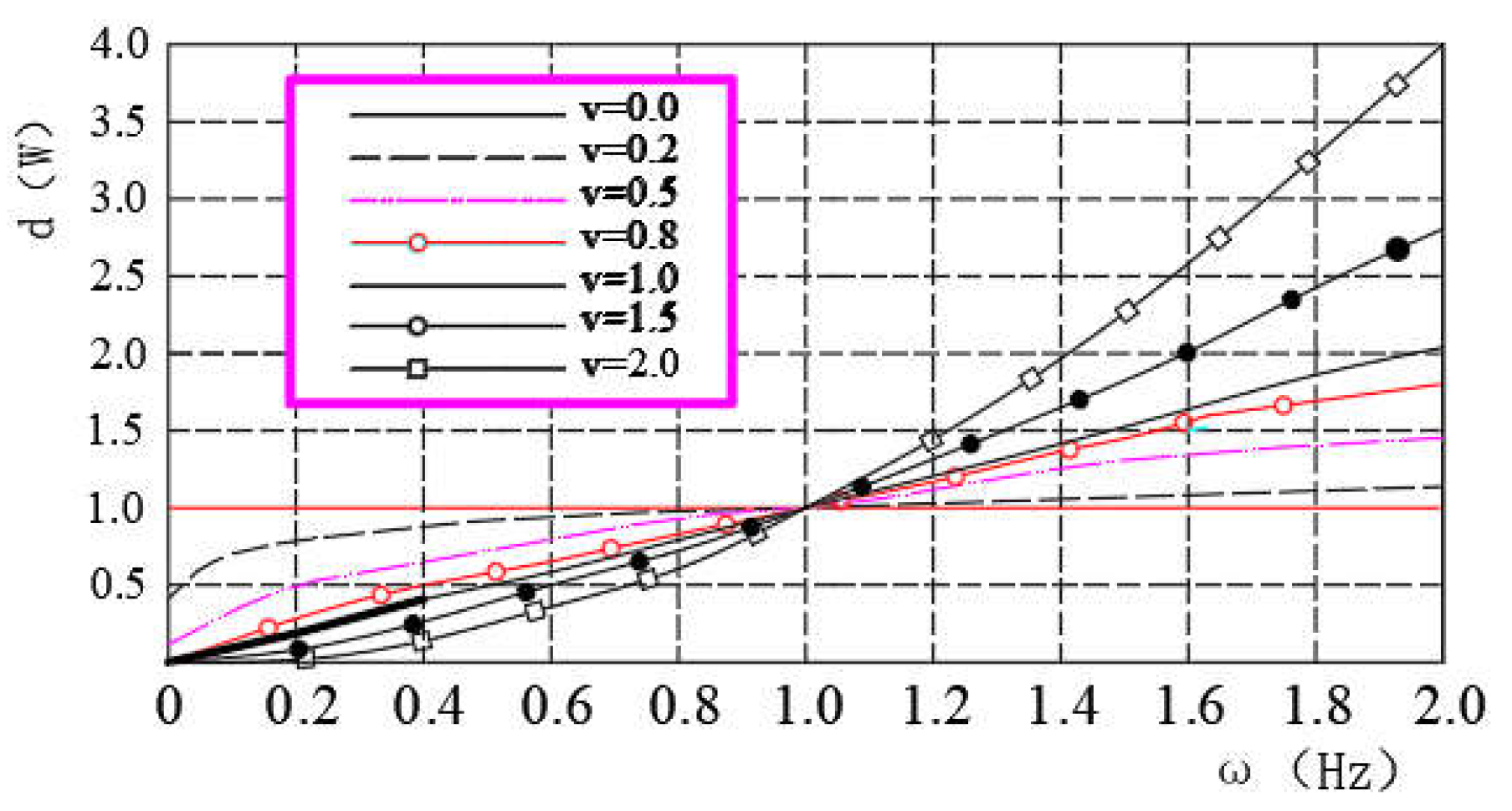
Figure 1. Spectral characteristic curve of the fractional differential operator.
Preprints 68857 g001
Figure 2. Distribution of information data of each sensor.
Preprints 68857 g002
Figure 3. Distribution curve of each measurement data.
Preprints 68857 g003
Table 1. Experimental data of the logistics robot spindle temperature (℃)
Number of sampling Sensor number Mean value Fj Standard
deviation Sjy
1# 2# 3# 4# 5# 6# 7# 8#
1st 53.00 53.10 52.75 53.10 52.80 53.60 57.66 52.65 53.12 0.30
2st 53.20 54.20 52.55 53.20 52.80 53.30 58.34 53.10 53.21 0.45
3st 53.00 53.40 48.43 52.96 53.20 53.80 52.70 53.60 53.09 0.38
4st 56.05 53.00 52.75 53.70 52.50 53.20 52.82 52.50 52.94 0.51
5st 47.35 53.30 52.80 53.50 46.52 53.62 53.05 53.15 53.17 0.34
6st 52.80 53.15 52.51 53.15 53.11 52.65 52.70 52.88 53.00 0.40
7st 53.50 53.52 52.54 53.20 52.90 53.80 53.15 53.12 53.16 0.49
8st 53.30 53.60 53.12 52.75 52.80 53.10 52.85 53.05 53.35 0.49
Mean value Fi 53.13 53.41 52.72 53.20 52.87 53.38 52.88 53.01 53.07
Standard deviation Six deviation Six 0.15 0.35 0.20 0.28 0.21 0.37 0.17 0.32
Mean value F 53.07
Mean standard deviation Sx 0.251 Mean standard deviation Sy 0.333 Total deviation T 1.580
Table 2. 0.5-order partial differential equation fusion values of measured data from each sensor (℃).
Number of sampling Sensor number
1# 2# 3# 4# 5# 6# 7# 8#
1st 63.731 64.151 63.834 63.993 63.854 64.182 63.772 64.079
2st 63.731 64.151 63.834 63.993 63.854 64.182 63.772 64.079
3st 63.731 64.151 63.834 63.993 63.854 64.182 63.772 64.079
4st 63.731 64.151 63.834 63.993 63.854 64.182 63.772 64.079
5st 63.731 64.151 63.834 63.993 63.854 64.182 63.772 64.079
6st 63.731 64.151 63.834 63.993 63.854 64.182 63.772 64.079
7st 63.731 64.151 63.834 63.993 63.854 64.182 63.772 64.079
8st 63.731 64.151 63.834 63.993 63.854 64.182 63.772 64.079
Table 3. 0.5-order partial differential equation fusion values of measured data from each sensor.
Number of sampling Sensor number
1# 2# 3# 4# 5# 6# 7# 8#
1st 59.776 59.776 59.776 59.776 59.776 59.776 59.776 59.776
2st 59.918 59.918 59.918 59.918 59.918 59.918 59.918 59.918
3st 59.828 59.828 59.828 59.828 59.828 59.828 59.828 59.828
4st 59.850 59.850 59.850 59.850 59.850 59.850 59.850 59.850
5st 59.761 59.761 59.761 59.761 59.761 59.761 59.761 59.761
6st 59.731 59.731 59.731 59.731 59.731 59.731 59.731 59.731
7st 59.836 59.836 59.836 59.836 59.836 59.836 59.836 59.836
8st 59.753 59.753 59.753 59.753 59.753 59.753 59.753 59.753
Table 4. The values of 0.5-order partial differential of the measured value of each sensor at different time points.
Number of sampling Sensor number
1# 2# 3# 4# 5# 6# 7# 8#
1st 61.754 61.964 61.805 61.885 61.815 61.979 61.774 61.928
2st 61.825 62.035 61.876 61.956 61.886 62.050 61.845 61.999
3st 61.780 61.990 61.831 61.911 61.841 62.005 61.800 61.954
4st 61.791 62.001 61.842 61.922 61.852 62.016 61.811 61.965
5st 61.746 61.956 61.798 61.877 61.808 61.972 61.767 61.920
6st 61.731 61.941 61.783 61.862 61.793 61.957 61.752 61.905
7st 61.784 61.994 61.835 61.915 61.845 62.009 61.804 61.958
8st 61.742 61.952 61.794 61.873 61.804 61.968 61.763 61.916
Mean value F0.5 61.878
Amplification factor K 61.878/53.07=1.166
Table 5. The final outcom of 0.5-order partial differential equation fusion values of measured data from each sensor (℃).
Number of sampling Sensor number Mean value
Fj
Standard
deviation Sjy0.5
1# 2# 3# 4# 5# 6# 7# 8#
1st 52.962 53.142 53.006 53.074 53.015 53.155 52.979 53.111 53.056 0.070
2st 53.023 53.203 53.067 53.135 53.075 53.216 53.040 53.172 53.116 0.070
3st 52.984 53.164 53.028 53.096 53.037 53.178 53.002 53.133 53.078 0.070
4st 52.994 53.174 53.038 53.106 53.046 53.187 53.011 53.143 53.087 0.070
5st 52.955 53.136 53.000 53.068 53.008 53.149 52.973 53.105 53.049 0.070
6st 52.943 53.123 52.987 53.055 52.995 53.136 52.960 53.092 53.036 0.070
7st 52.988 53.168 53.032 53.100 53.040 53.181 53.005 53.137 53.081 0.070
8st 52.952 53.132 52.996 53.064 53.005 53.145 52.970 53.101 53.046 0.070
Mean value Fi 52.975 53.155 53.019 53.087 53.028 53.168 52.993 53.124 53.069 0.070
Standard deviation Six0.5 0.026 0.025 0.025 0.025 0.025 0.025 0.025 0.025
Mean standard deviation Sx0.5 0.025 Mean standard deviation Sy0.5 0.070 Total deviation T0.5 0.175
Disclaimer/Publisher’s Note: The statements, opinions and data contained in all publications are solely those of the individual author(s) and contributor(s) and not of MDPI and/or the editor(s). MDPI and/or the editor(s) disclaim responsibility for any injury to people or property resulting from any ideas, methods, instructions or products referred to in the content.
Copyright: This open access article is published under a Creative Commons CC BY 4.0 license, which permit the free download, distribution, and reuse, provided that the author and preprint are cited in any reuse.
Prerpints.org logo

Preprints.org is a free preprint server supported by MDPI in Basel, Switzerland.

Subscribe

© 2024 MDPI (Basel, Switzerland) unless otherwise stated