Improving Foraminifera Classification Using Convolutional Neural Networks with Ensemble Learning

Preprint

Article

Improving Foraminifera Classification Using Convolutional Neural Networks with Ensemble Learning

Altmetrics

Downloads

170

Views

Comments

Loris Nanni^*,Giovanni Faldani,

Sheryl Brahnam

Riccardo Bravin

Elia Feltrin

Loris Nanni^*,Giovanni Faldani,

Sheryl Brahnam

Riccardo Bravin

Elia Feltrin

This version is not peer-reviewed

Submitted:

20 February 2023

Posted:

23 February 2023

You are already at the latest version

Alerts

Abstract

This paper presents a study of an automated system for identifying planktic foraminifera at the species level. The system uses a combination of deep learning methods, specifically Convolutional Neural Networks (CNNs), to analyze digital images of foraminifera taken at different illumination angles. The dataset is composed of 1437 groups of sixteen grayscale images, one group for each foraminifer, that are then converted to RGB images with various processing methods. These RGB images are fed into a set of CNNs, organized in an Ensemble Learning (EL) environment. The ensemble is built by training different networks using different approaches for creating the RGB images. The study finds that an ensemble of CNN models trained on different RGB images improves the system's performance compared to other state-of-the-art approaches. The proposed system was also found to outperform human experts in classification accuracy.

Keywords:

Subject: Computer Science and Mathematics - Artificial Intelligence and Machine Learning

1. Introduction

Image classification is a very complex task that has witnessed massive improvement in the past decade thanks to hardware advancements and the application of Deep Learning. Because this new technology is a repetitive and non-creative process, it is well-suited for automation. One of the best deep learners for images is a family of learners called Convolutional Neural Networks (CNNs). CNNs have already proven their efficacy and efficiency at image classification in many studies [1]; however, the stochastic nature of neural networks (NNs) leads to results that are influenced by a fair share of randomness [2]. Ensemble Learning (EL) is a widely used implementation that combines results from different networks to achieve better performance and higher consistency, reducing the individual random component of each network. Transfer learning, which takes a pre-trained CNN as the baseline for training yet another dataset of images, typically a smaller one, is yet another technique that can be employed to improve classification accuracy both at the first epoch and at the end of the training process.

This paper proposes a practical application of EL to the classification problem presented in [3], which was to train a CNN for foraminifera classification, a task of high interest for industrial and research purposes. Species of planktic foraminifera are paleo-environmental bioindicators whose radiocarbon measurements are used to infer parameters like global ice volume, temperature, salinity, PH, and nutrient content of ancient marine environments. Foraminifera classification is usually performed by groups of humans, ranging in size from 500 to 1000 individuals. As a result, foraminifera classification is a very repetitive, resource-intensive, and time-consuming process. In the early 1990s, there have been several attempts to automate this task. Although strides were made in this direction, most methods still required strong human supervision. In 2004, however, the neural network SYRACO2 was developed to identify single-celled organisms automatically and was shown to perform reliably [4]. In 2017 CNNs were applied to diatom identification with great success [5]. With further development, CNNs should be able to take over the arduous process of foraminifera classification.

Our goal is to improve the classification accuracy on the same dataset presented in [3]. This dataset is composed of 1437 groups of sixteen grayscale images of foraminifera taken at different lighting angles and separated into seven classes. Several RGB colorization approaches were used to generate different sets of colored images that became the inputs for a set of CNN architectures that formed the EL environment. The authors of [3] employed a fusion of ResNet50 and Vgg16, using colorization methods based on intensity percentiles in the sixteen grayscale channels.

This paper proposes several alternative colorization methods that deviate from the state of the art [6] but still achieve remarkable ensemble results. New approaches such as Luma scaling, HSV colorspace mapping, and gaussian or mean-based techniques are applied to CNN architectures to extend [3]. The results of this study show that a diverse set of CNN models trained on different colorized images improves the system's performance compared to other state-of-the-art approaches. The proposed system is also shown to outperform human experts in classification accuracy.

It's important to note that the application of multi-grayscale channels to RGB colorization is not limited to the field of foraminifera classification but can be applied in other domains as well. Some example applications include remote sensing [7,8], where multispectral images are often represented in grayscale, and medical imaging, where grayscale images are commonly used in CT scans and MRI images [9]. The use of RGB colorization in these domains has already been shown to improve the performance of classification tasks and enhance the interpretability of the results. For example, in medical imaging, converting grayscale images to RGB can highlight certain features in the images that were not as noticeable in grayscale, potentially leading to improved diagnosis accuracy [10]. Similarly, in remote sensing, RGB colorization can help highlight different features in the image, such as vegetation or water bodies, improving CNNs results. Thus, the methods proposed here should also increase classification accuracy in other domains that use grayscale images. Furthermore, our methods should work well for the image fusion of different grayscale pictures obtained from multispectral analysis or from polarized/filtered light sources on objects that may be difficult to capture in the typical visible spectrum.

2. Convolutional Neural Networks

CNNs were first introduced in the 1980s by the French researcher Yann LeCun [11] and were shown to perform well throughout the 1990s [12,13]. In the last decade, however, due to the advent of big data and GPU computing, the performance of CNNs has increased to the point that in computer vision and image recognition CNNs are now considered state-of-the-art.

As with every other type of neural network, the structure of a CNN is divided into three components: an input layer, which, in a CNN architecture, is usually a volume of n×n×3 neurons directly connected to the input of an image's pixels, hidden layers that utilize shared weights and local connections, and a fully connected output layer.

CNNs implement pooling and convolution directly through the architecture. Local connections, non-linear activation functions, and shared weights are used to build feature maps that autonomously create the filters needed. Local connections and shared weights are what distinguish CNNs from a normal multilayer perceptron (MLP) network. Neurons of the hidden layers are only connected locally to the adjacent neurons, meaning they will only process information from a subset of the previous layer. Furthermore, weights and biases are shared in groups to interpret in a consistent manner information gained in different portions of the input. Convolution utilizes a digital filter (or mask) to extract data from a subset of the input. The result of filtering the whole input volume by making the mask slide in every possible position is a feature map [14]. Pooling is another filtering method that aggregates portions of an input feature map and is used to reduce variance between small transformations of the input [15]. Two of the most utilized methods are max and average pooling, from which the maximum or average value is extracted, given a portion of the input only.

The output layer of a CNN is a fully connected one that utilizes a neuron for each class, which is usually, in modern models, a SoftMax activation function:

{f (z)}_{k} = \frac{e^{z_{k}}}{\sum_{j = 1}^{n} e^{z_{j}}} .

with

n

, the number of classes and

z

the input vector. The function's output is a normalized value

0 \leq b \leq 1

and can be interpreted as confidence.

In this work, we use the ResNet50 topology pretrained using ImageNet, which is fine-tuned further for 20 epochs with a learning rate of 0.001 and a batch size of 30.

3. CNN Ensemble Learning

The theory behind Ensemble Learning is based on a simple idea: by combining different models, it should be possible to produce better and more reliable results. Ensembles can be constructed on four different levels:

Data level: by splitting the dataset into different subsets;
Feature level: by pre-processing the dataset with unique methods;
Classifier level: by training different classifiers on the same dataset;
Decision level: by combining the decisions of multiple models.

Ensembles work best when applied to significantly diverse models [16]. In this work, we construct ensembles by applying different pre-processing approaches, detailed in section 3.1, for representing the input images as RGB images. The images generated by these approaches are used to train multiple networks whose decisions are finally combined using the sum rule.

3.1. Image Pre-Processing

Each image in the dataset, presented in [3] and described in more detail in section 4, comes in the form of sixteen grayscale pictures of the same foraminifera subject. The dataset, size 1437 samples, is divided into seven classes: one for each of the six species of foraminifera that are the subject of this study. Each class has approximately 150 entries, except for the last which has 450.

Since we use pre-trained networks and their inputs are expected to be RGB images, the first step in our pipeline will be to generate CNN-compatible inputs starting from the dataset.

Multiple ways for completing this task were tested; in the end, we settled on a combination of five:

The "Percentile" method presented in [3], also called "Baseline".
A "Gaussian" image processing method that encodes each color channel based on the normal distribution of the grayscale intensities of the sixteen images.
Two "Mean-based" methods focused on utilizing an average or mean of the sixteen images to reconstruct the R, G, and B values.
The "HSVPP" method that utilizes a different color space composed of hue, saturation, and value of brightness information.

An illustration of the resulting images can be found in Figure 3. A discussion of the five methods is provided below.

3.1.1. Percentile

Percentile is the most straightforward method for generating an RGB image. As presented in [3], the sixteen individual grayscale values for each pixel are used to calculate the 10th percentile, median, and 90th percentile. These three values are then mapped to the RGB channels to generate a single color composite.

To speed up the process, we use the nearest rank method: the list of sixteen grayscale values is sorted in ascending order, after which the P-th percentile element is selected by extracting the value of cell

n

, where

n = ⌈\frac{P}{100} \cdot 16⌉ .

Since our input vectors are always the same size, the sixteen values are sorted, and the three values of

n

selected here are 2, 8, and 15.

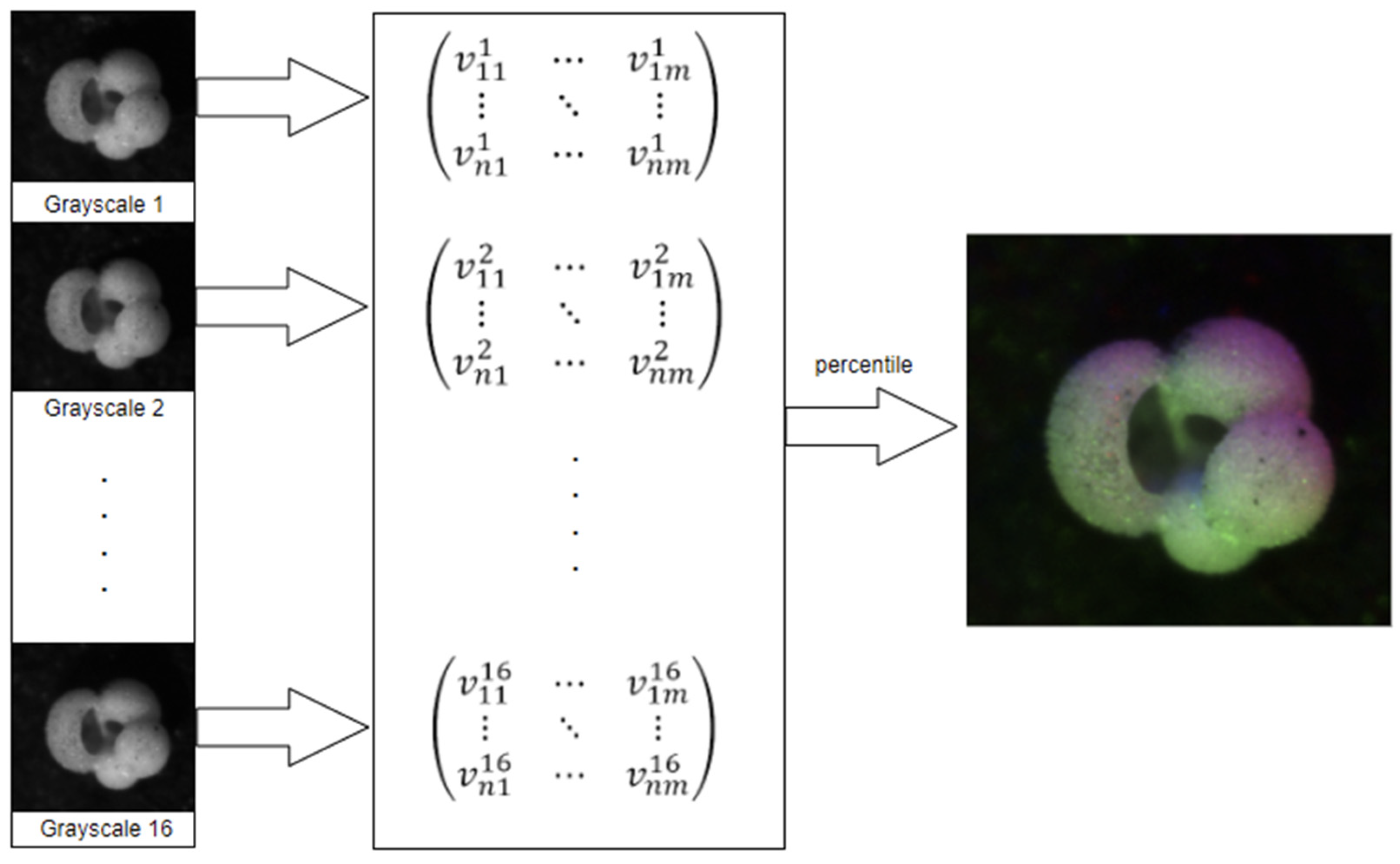
The percentile pre-processing pipeline, see Figure 1, works as follows:

Read the sixteen images;
Populate a $N \times M \times 16$ matrix with the grayscale values;
For each pixel, extract its sixteen grayscale values into a list;
Sort the list;
Use elements 2, 8, and 15 as RGB values for the new image;

Figure 1. Percentile pre-processing pipeline, sourced from [17].

A few variations of this method were also tested (the 20th/80th/median, for example), but they were discarded due to their performance being slightly worse than the original, losing out on 1-2% of accuracy per single-run training cycle on average.

3.1.2. Gaussian

The Gaussian method for image processing tries to find the optimal way to fit the sixteen grayscale image values at position

x

, represented as the vector

I_{16} (x)

, in a normal distribution, using the fitdist method in MATLAB.

The fitting of sixteen values into a normal distribution is independent of their ordering, thereby ensuring that no bias from the order of lighting angles is encoded into the colorized images.

Once the distribution is computed, the R, G, and B values of the colorized image are assigned as follows:

Given the gaussian random variable

X ~ N (μ, σ)

fit from

I_{16} (x)

R (x) = μ - 2 σ G (x) = μ B (x) = μ + 2 σ

If any assigned value is negative or exceeds 255, it is thresholded to the nearest valid color intensity value 0 or 255.

3.1.3. Mean-based

With mean-based methods, the main idea is to address the lack of ordering in the lighting angle of the various samples by combining the sixteen pictures of each sample into a single image that approximates the information contained in the grayscale images. The mean is then used to determine each of the RGB color values. The advantage of approaches like these is that they can be computed relatively quickly compared to more involved image colorization techniques. The techniques used to determine the RGB color values are detailed in the following sub-sections. Given a set of values

S = \{x_{1}, \dots, x_{n}\}

, the following means were calculated:

$A r i t h m e t i c M e a n (S) = \frac{1}{n} \sum_{i = 1}^{n} x_{i}$
$G e o m e t r i c M e a n (S) = {(\prod_{i = 1}^{n} x_{i})}^{\frac{1}{n}}$
$H a r m o n i c M e a n (S) = {(\frac{\sum_{i = 1}^{n} {x_{i}}^{- 1}}{n})}^{- 1}$

3.1.3.1. Luma Scaling

Considering that a mean grayscale image can be viewed as containing only luminosity information, it follows that a possible way to assign RGB values and colorize the picture would be to try to compute a color value according to its perceived luminosity. With images close to the resolution of Standard Definition (SD) television, which is 704×480 pixels, the Luma Scaling approach attempts to encode luma information in the component video following values used by the BT.601 standard. The formula for recovering luma information is:

Y^{'} = 0.299 \cdot R + 0.587 \cdot G + 0.114 \cdot B

This formula weighs the primary colors based on their brightness, with green the brightest component and blue the dimmest. The Luma Scaling images are obtained from these weights, which are multiplied by the mean image to get the intensity value for each color channel; the result is a basic recoloring obtained by computing the following:

Given the pixel at position

x

, let

I_{16} (x)

be the array of sixteen values of the grayscale intensity of the sixteen images in that position; the colored reconstruction is obtained as follows:

$R (x) = 0.299 \cdot A r i t h m e t i c M e a n (I_{16} (x))$
$G (x) = 0.587 \cdot A r i t h m e t i c M e a n (I_{16} (x))$
$B (x) = 0.114 \cdot A r i t h m e t i c M e a n (I_{16} (x))$ .

3.1.3.2. Means Reconstruction

This approach utilizes an important relationship between the three different means. Knowing that the order of luminosity between the three primary colors is

B l u e < R e d < G r e e n

and given an array of real numbers

S

, the following relationship holds true:

M i n (S) \leq H a r m o n i c M e a n (S) \leq G e o m e t r i c M e a n (S) \leq A r i t h m e t i c M e a n (S) \leq M a x (S) .

Given the vector of sixteen grayscale images of each sample

I_{16} (x)

at a given pixel position

x

, the Means Reconstruction approach maps every mean to a color channel according to the established order as follows:

$R (x) = G e o m e t r i c M e a n (I_{16} (x))$
$G (x) = A r i t h m e t i c M e a n (I_{16} (x))$
$B (x) = H a r m o n i c M e a n (I_{16} (x))$ .

3.1.3. HSVPP: Hue, Saturation, Value of brightness + Post-Processing

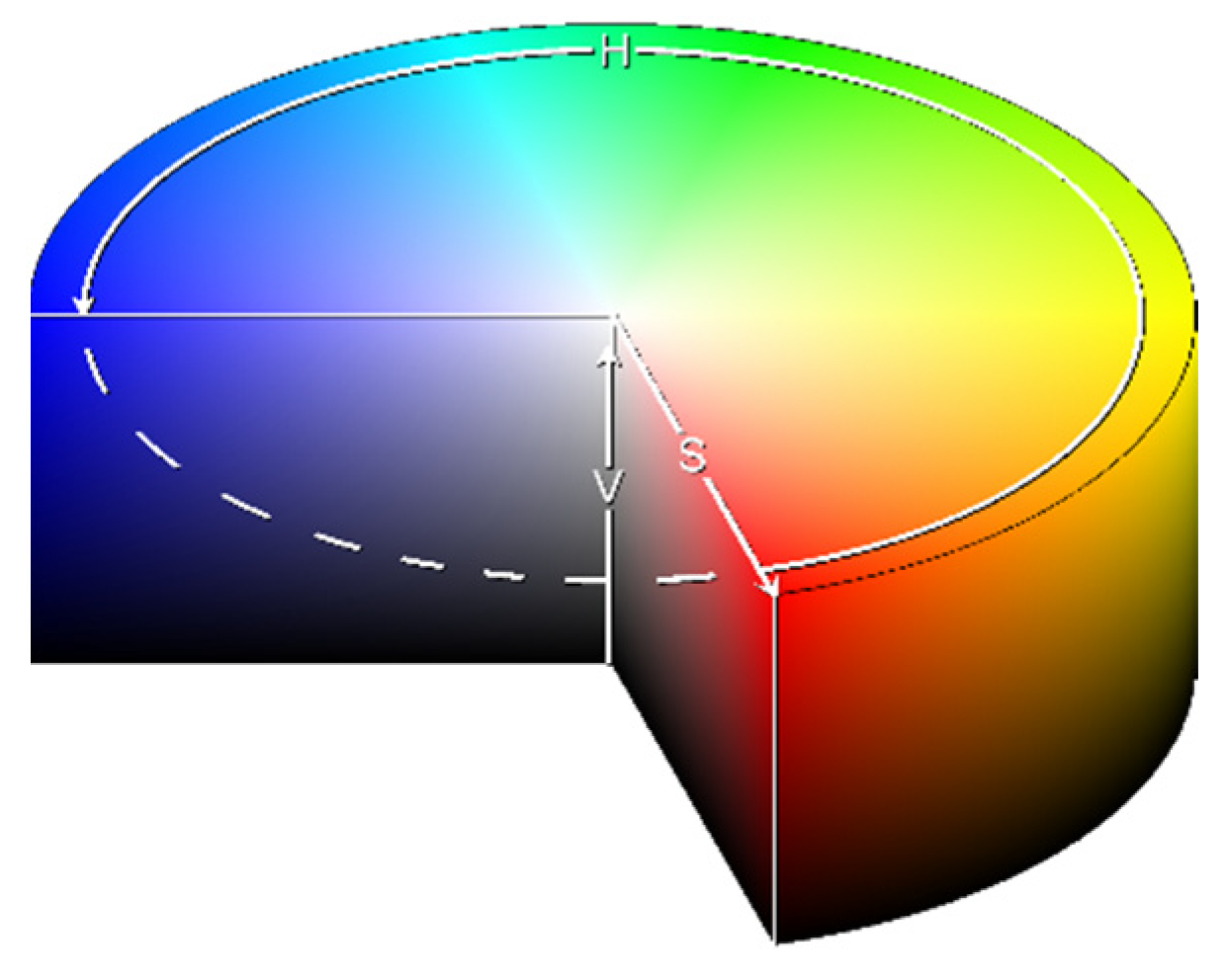
This method utilizes an alternative representation of RGB information. Instead of encoding each RGB color channel separately, each pixel is encoded with three different values that represent coordinates in the HSV color space, as illustrated in Figure 2.

To encode the three values this conversion is used:

Hue (H) encodes the angle of the color vector on the HSV space, with 0° being red, 120° being green, and 240° being blue, rescaled to [0,1] during computation;
Saturation (S) determines how far from the center of the circumference the color is placed in the range [0,1];
Value of brightness (V) calculates the height in the color space cylinder and measures color luminosity in the range [0,1].

The three values are computed for all sixteen grayscale images in the following manner:

H is assigned based on the index of the image, giving each a different color hue;
S is set to 1 by default, for maximum diversity between colors;
V is set to the grayscale image's original intensity, i.e., its brightness.

Since the ordering of the lighting angles differs across the classes, the sixteen images are shuffled randomly to prevent bias before computing H. Shuffling ensures that the network does not discriminate classes based on the order of lightning angles in the post-processed images.

After obtaining sixteen images of different colors, they are fused into a single RGB image by converting the HSV representation to RGB and then by summing the squared intensity of each channel together into a single colorized image.

Finally, it is possible to enhance the resulting images with some post-processing, mainly by increasing the brightness of the darker colors and reducing haze for a sharper image. Once this post-processing is done, the HSVPP dataset is ready to be fed to the network.

Figure 3. Examples of the six colorization methods. In the top row from left to right: Percentile, Gaussian, and Luma Scaling images; In the bottom row from left to right: Means Reconstruction, HSV, and HSVPP images.

3.2. Training

Once the dataset is built, networks are trained using a pre-trained ResNet50, which, as the name suggests, is a 50-layer CNN. The input layer is a 224×224×3 zero-pad layer. There are 48 hidden layers, two of which are a max and an average pool, respectively. Networks of the ResNet family utilize residual blocks to maximize depth while diminishing the number of parameters [19]. The output layer is a 1000-neuron SoftMax layer.

All networks were pre-trained with the open-source image dataset ImageNet, which contains millions of labelled images. Hyperparameters for all networks were set as follows:

Mini Batch Size: 30
Max Epochs: 20
Learning Rate: 10^-3

The main benefit of a pre-trained network is transfer learning. A modern neural network can carry over some of the knowledge gained in previous training cycles on a particular dataset when retraining it on a different dataset [19] . This carry-over of information is especially pronounced in deep learning models because they operate on a wide array of weights and features. Transfer learning significantly reduces the time and number of images needed to train the networks, an advantage when working with relatively small datasets.

The output layer of the pretrained networks has to be adapted to accommodate the task of foraminifera classification. Thus, all the output layers were replaced with fully connected SoftMax layers of seven neurons, one for each class of foraminifera available in the dataset. Images of the dataset were also resized to match the dimensions of the input layers.

By replacing the last layer with a seven-neuron SoftMax layer, the outputs form a vector

v

, whose values (scores) are:

\{\begin{matrix} 0 \leq v_{i} \leq 1 \forall i \\ \sum_{i = 1}^{7} v_{i} = 1 \end{matrix} .

Scores reflect the level of confidence with which the networks classify an input.

By diversifying the models, the information processed by each is different. Score fusion is a method that combines the confidence values of each model to build a more robust prediction. The fusion technique used here is the sum rule [16], defined as:

s u m = \sum_{i = 1}^{N} v; o u t = a r g m a x \{{s u m}_{j}\}, j = 1 \dots n

where

N

is the number of models and

n

the size of each confidence vector

v

. The sum rule is one of the best fusion methods because it does not suffer from potentially destructive operations like multiplication by zero.

4. Results

The dataset used for all tests is composed of a total of 1437 samples, divided into the following classes:

178 images are G. bulloides;
182 images are G. ruber;
150 images are G. sacculifer;
174 images are N. incompta;
152 images are N. pachyderma;
151 images are N. dutertrei;
450 images are "rest of the world," i.e., they belong to other species of planktic foraminifera.

The initial images were obtained using a reflected light binocular microscope, each taken with a light shining from the side at 22.5° intervals, using an AmScope SE305R-PZ binocular microscope at 30× magnification [3]. For every sample of foraminifera, sixteen grayscale pictures were taken at different illumination angles. The resolution of the images can vary per sample, but most are around 450×450 pixels. Upon manual inspection, the starting illumination angle for the sixteen images seems to change partially for different classes of foraminifera in the naming scheme used to sort the pictures. We believed the start angle could lead to biased results in classification if a specific class always had the same starting angle compared to the others. This problem was addressed, when pre-processing the images, by randomly sorting them while keeping the relative illumination angles ordered to avoid the insertion of bias within methods that leverage the light positional information.

The testing protocol for the dataset is the 4-fold cross-validation, and the performance metric is the F-score (

F_{1}

), defined as:

F_{1} = \frac{T_{p}}{T_{p} + \frac{1}{2} (F_{p} + F_{n})}

where

T_{p}

F_{p}

F_{n}

are respectively the total number of True positives and the False positive/negative predictions made by the model.

In Table 1, we compare our ensemble with that proposed in [3]. With

X (y)

, we report the performance of

y

ResNet50 trained with the

X

RGB approach for colorizing the images.

The conclusions that can be obtained from the results reported in Table 1 are the following:

The best-performing ensemble produces results that significantly improve those obtained by the method presented in [3] (Percentile), whose $F_{1}$ score was reported as 81%.
It appears that, in general, increasing the diversity of the ensemble yields better results. The approaches combining multiple preprocessed images sets consistently rank higher in $F_{1}$ scores than any individual method, iterated ten times. Combining fewer iterations of all the approaches yielded the best results overall.

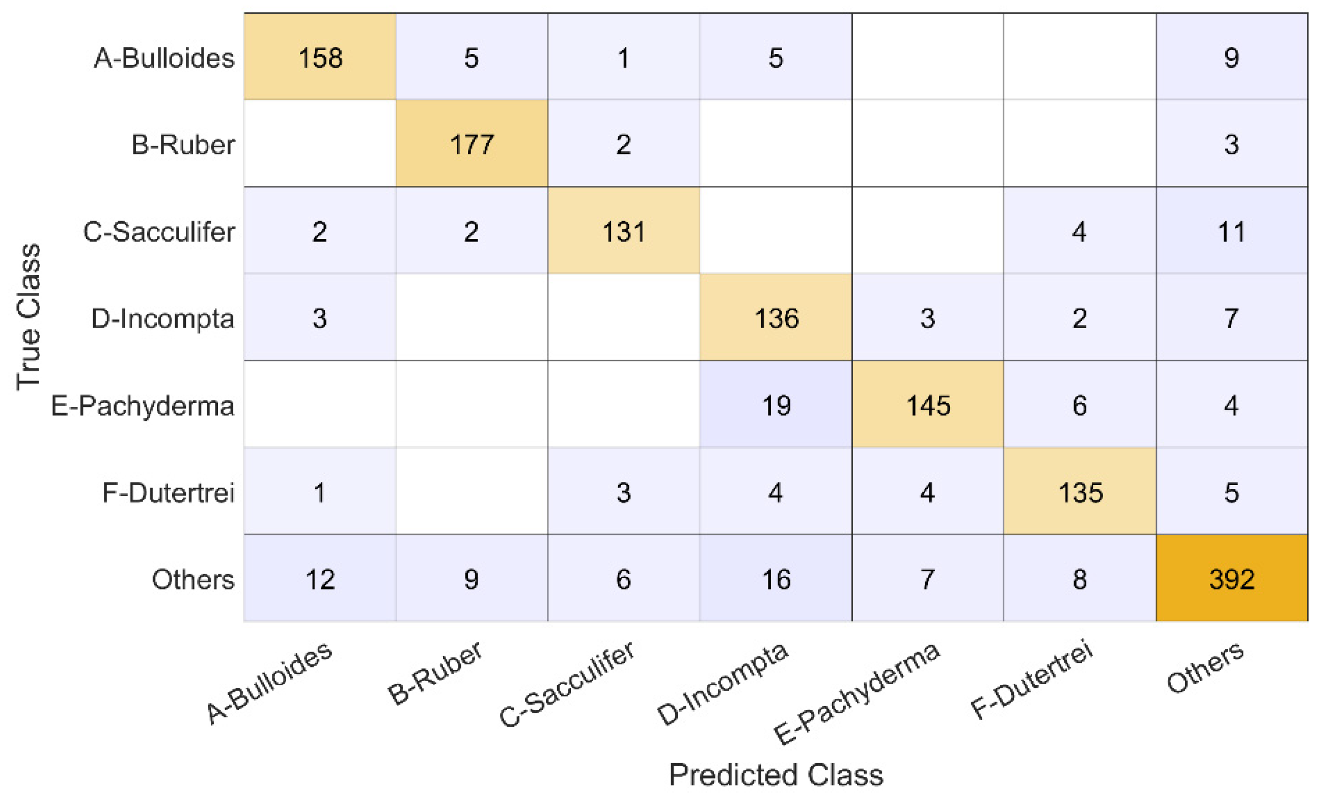
The breakdown of the 4-fold classification on the full dataset is presented in Figure 4 as a confusion chart, where we can see the number of true positives, false positives, and false negatives. The G. sacculifer was the class classified correctly the least, but this class had the smallest number of samples, 150 specimens, compared to the rest, which could have affected results. Also noteworthy is the high number of false positives predicted for the N. incompta class, consistent with the classification rate in [3], although if found the false negatives to be the larger issue.

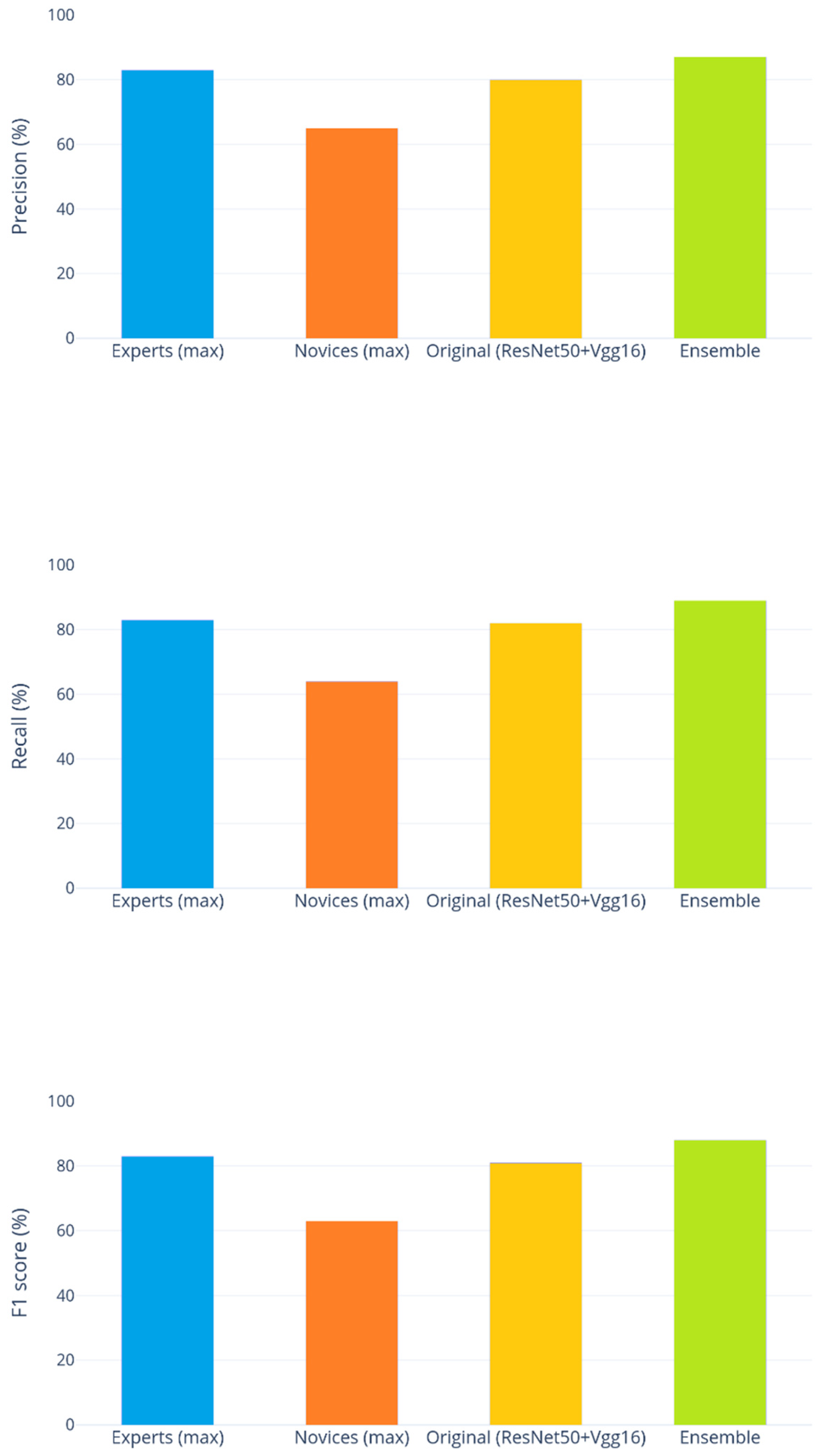
Comparing the final results of the ensemble with the study reported in [3], the precision averaged across the six labelled classes achieved by six human experts ranged from 59% to 83%, with a mean of 74%. In contrast, five human novices ranged from 49% to 65%, with 56% on average. The ensemble approach proposed in [3] was found to achieve an average precision of 80%, which is comparable to that of the experts. The best ensemble presented in Table 1, which is Percentile(2)+Gaussian(2)+Luma Scaling(2)+Means Reconstruction(2)+HSVPP(2), was found to achieve an average precision of 87%, a much better average than that of the experts and higher than any of them individually.

Similar results have been obtained for recall and the

F_{1}

score, which was always averaged across the six labelled classes. The six experts achieved recall between 32% and 83% (mean 60%), while the novices scored 47%–64% (mean 53%). The ensemble proposed in [3] (named Original(ResNet50+Vgg16) in the following figures) reported an average recall of 82%, while our ensemble reached 89%. The

F_{1}

score of the six experts ranged from 39% to 83% (mean 63%), the five novices obtained

F_{1}

scores between 47% and 63% (mean 53%), and the [3] reported an average of 81%. The ensemble presented in this paper scored 88%. These results are illustrated in Figure 5.

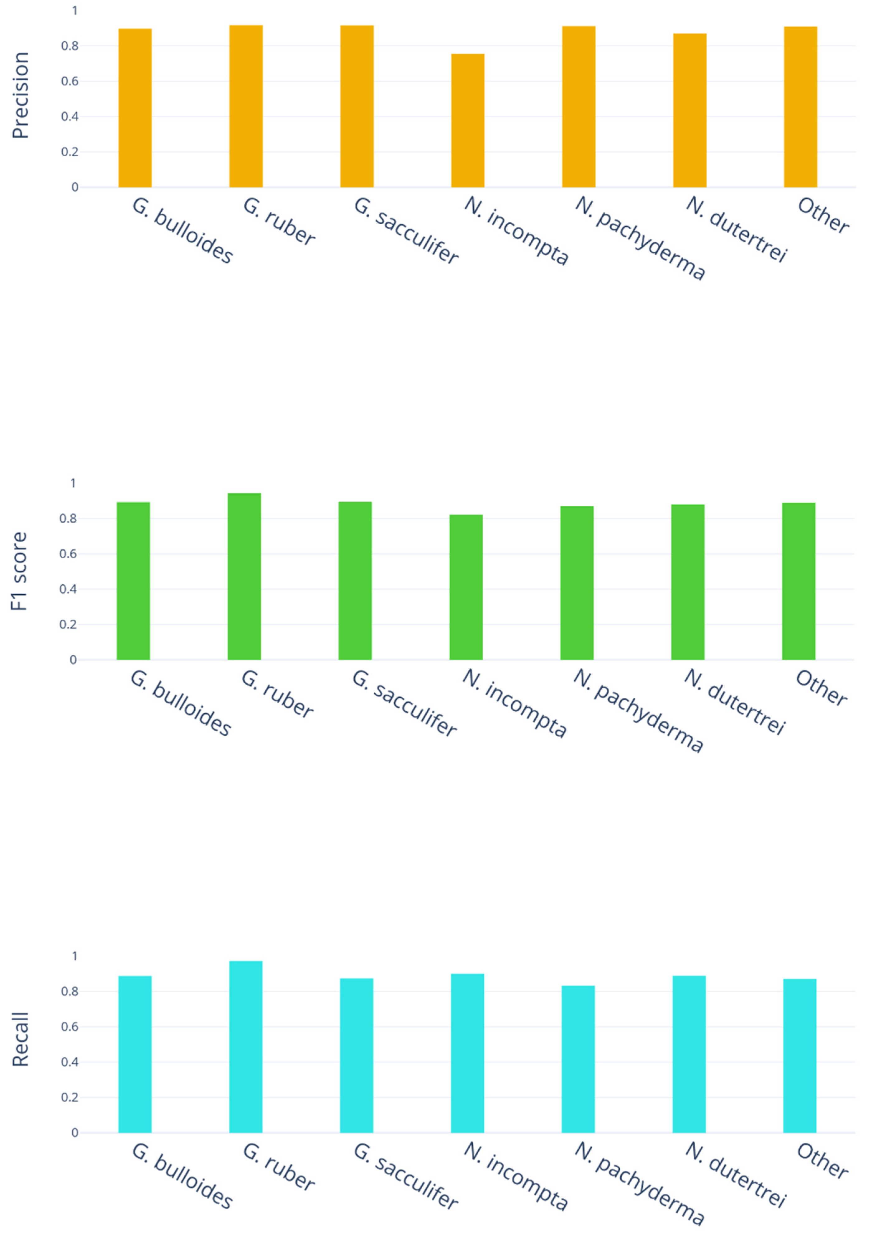
On a finer level, we have also charted the precision, recall and

F_{1}

scores across all the different classes in our study, as seen in Figure 6.

In both precision and

F_{1}

score, N. incompta comes out the lowest by a significant margin, achieving 0.76 in precision, while the other six classes average 0.9; the

F_{1}

score for N. incompta is 0.82, while the other six classes average 0.88. N. pachyderma has the poorest recall, achieving 0.83, while the other six classes average 0.9. In contrast, the highest precision, recall, and

F_{1}

score were all achieved on the G. ruber class, which may indicate it has features that are easier to distinguish than all the others.

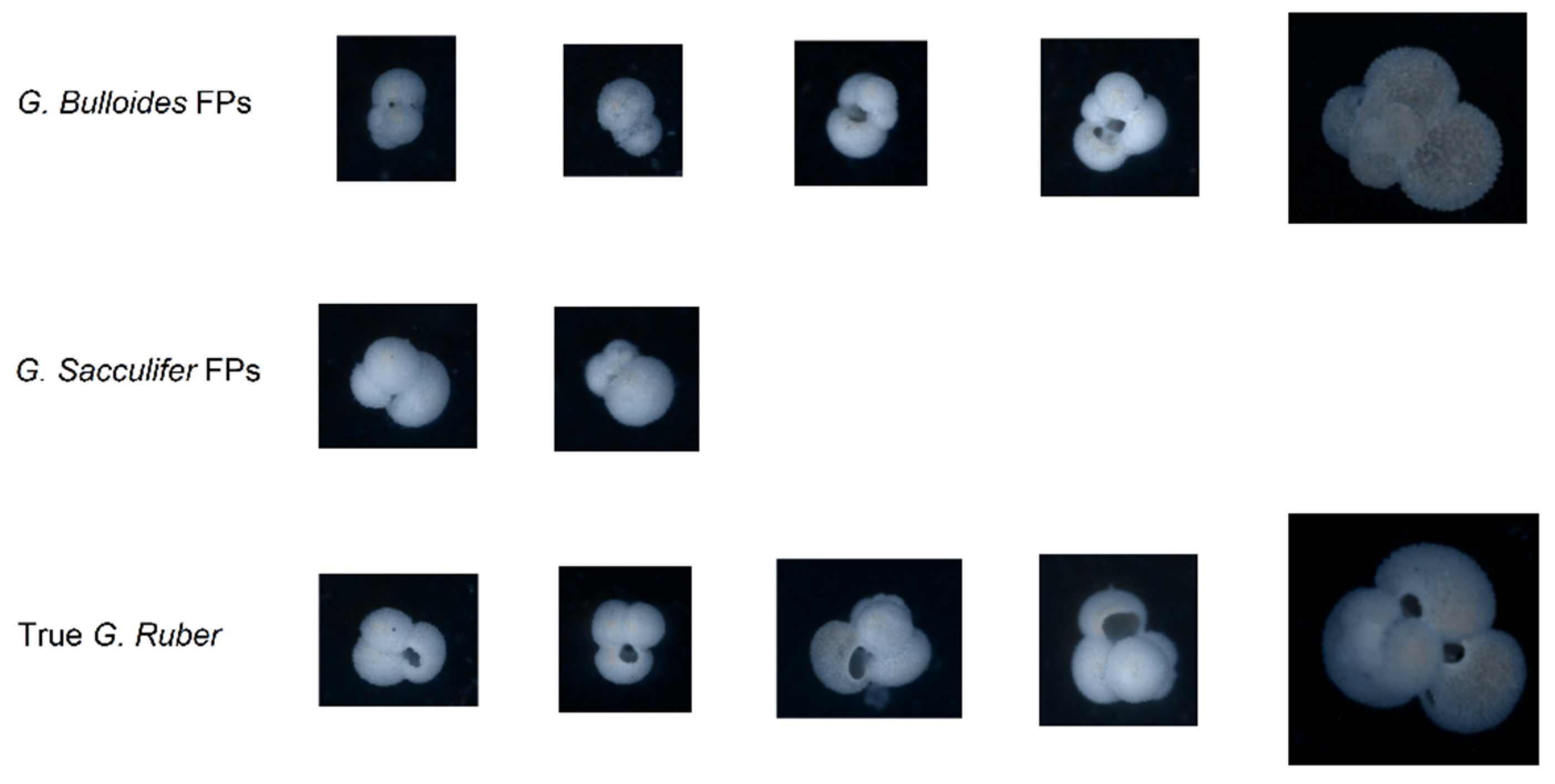
Out of the false positives for G. ruber, two were G. sacculifer, five were G. bulloides, and nine were Others, while the false negatives were only misclassified as G. sacculifer or as Other. The differences and similarities between the false positives and real data are illustrated in Figure 7.

It's important note that all the performance indicators for our method achieved scores higher than 75%, while in [3] some classes like N. dutertrei had precision less than 70%.

5. Conclusions

Although the sample size of the experiment is small, the impact of Ensemble Learning on the problem is definitely noticeable. There are, however, a few points of concern. The dataset only contained ~1500 images divided into seven classes of foraminifera, a problem we addressed with transfer learning. Nonetheless, the scope of the experience was limited to a very small portion of the real-world problem of foraminifera classification. We can, however, safely assume that with more samples per class, performance could be enhanced even further. What we are uncertain about, without experimental data, is how the model would respond to a larger set of classes. Image preprocessing and classification on multiple CNNs are very time-consuming tasks. Because our models were run on sub-optimal machines, our focus was directed toward maximizing accuracy while neglecting the time it took for training.

A possible future development of the project is the application of the technique used to generate an approximate normal map of an object from grayscale images with lights coming from the four cardinal directions. Since normal maps are used in 3D computer graphics to fake details such as bumps, dents, and lighting without the need for added geometry, these results could also be used to generate entirely new images with new lighting conditions, colors, and viewpoints without the need of the human labor usually needed to increase the size of the dataset.

Author Contributions

Conceptualization, L.N and G.F.; methodology, L.N; software, R.B., E.F., L.N and G.F.; investigation, L.N, S.B, R.B., E.F and G.F.; writing—original draft preparation, R.B., E.F, S.B., G.F. and L.N; writing—review and editing, S.B., G.F. and L.N.

Funding

This research received no external funding.

Data Availability Statement

https://doi.pangaea.de/10.1594/PANGAEA.897873.

Acknowledgments

Through their GPU Grant Program, NVIDIA donated the TitanX GPU used to train the CNNs presented in this work.

Conflicts of Interest

The authors declare no conflict of interest.

References

Zewen Li, Fan Liu, Wenjie Yang, Shouheng Peng and Jun Zhou, A Survey of Convolutional Neural Networks: Analysis, Applications, and Prospects, 2021. [CrossRef]
Christopher Menart, Evaluating the variance in convolutional neural network behavior stemming from randomness, 2020. [CrossRef]
R. Mitra, T.M. Marchitto, Q. Ge, B. Zhong, B. Kanakiya, M.S. Cook, J.S. Fehrenbacher, J.D. Ortiz, A. Tripati, E. Lobaton, Automated species-level identification of planktic foraminifera using convolutional neural networks, with comparison to human performance, 2019. [CrossRef]
Luc Beaufort, Denis Dollfus, Automatic recognition of coccoliths by dynamical neural networks, 2004. [CrossRef]
Luis F. Pedraza, Cesar A. Hernández, Danilo A. López, "A Model to Determine the Propagation Losses Based on the Integration of Hata-Okumura and Wavelet Neural Models", International Journal of Antennas and Propagation, vol. 2017, Article ID 1034673, 8 pages, 2017. [CrossRef]
Bing Huang, Feng Yang, Mengxiao Yin, Xiaoying Mo, Cheng Zhong, "A Review of Multimodal Medical Image Fusion Techniques", Computational and Mathematical Methods in Medicine, 2020. [CrossRef]
Akrem Sellami, Ali Ben Abbes, Vincent Barra, Imed Riadh Farah, Fused 3-D spectral-spatial deep neural networks and spectral clustering for hyperspectral image classification, Pattern Recognition Letters, Volume 138, 2020. [CrossRef]
Xingchen Zhang, Ping Ye, Gang Xiao, VIFB: A Visible and Infrared Image Fusion Benchmark, Proceedings of the IEEE/CVF Conference on Computer Vision and Pattern Recognition (CVPR) Workshops, 2020, pp. 104-105.
Alex Pappachen James, Belur V. Dasarathy, Medical image fusion: A survey of the state of the art, Information Fusion, Volume 19, 2014. [CrossRef]
Sarmad Maqsood, Umer Javed, Multi-modal Medical Image Fusion based on Two-scale Image Decomposition and Sparse Representation, Biomedical Signal Processing and Control, Volume 57, 2020. [CrossRef]
Y. LeCun et al., "Backpropagation Applied to Handwritten Zip Code Recognition," in Neural Computation, vol. 1, no. 4, pp. 541-551, Dec. 1989. [CrossRef]
Bengio, Y. & Lecun, Yann, Convolutional Networks for Images, Speech, and Time-Series, 1997.
Y. LeCun, L. Bottou, Y. Bengio and P. Haffner, "Gradient-based learning applied to document recognition," in Proceedings of the IEEE, vol. 86, no. 11, pp. 2278-2324, Nov. 1998. [CrossRef]
Xingchen Zhang, Ping Ye, Henry Leung, Ke Gong, Gang Xiao, Object fusion tracking based on visible and infrared images: A comprehensive review, Information Fusion, Volume 63, 2020. [CrossRef]
Ian Goodfellow, Yoshua Bengio, Aaron Courville, Deep Learning, The MIT Press, 2016.
Kuncheva L.I. Combining Pattern Classifiers. Methods and Algorithms, Wiley, 2nd edition, 2014.
http://hdl.handle.net/20.500.12608/29285.
https://it.wikipedia.org/wiki/Hue_Saturation_Brightness.
Fuzhen Zhuang, Zhiyuan Qi, Keyu Duan, Dongbo Xi, Yongchun Zhu, Hengshu Zhu, Hui Xiong, Qing He, A Comprehensive Survey on Transfer Learning. [CrossRef]

Figure 2. HSV color space representation as found on [18].

Figure 4. Confusion chart of the 4-fold cross validation results obtained by our ensemble.

Figure 5. Precision, recall and

F_{1}

score comparison between [3] and the best ensemble presented in the paper.

Figure 5. Precision, recall and

F_{1}

score comparison between [3] and the best ensemble presented in the paper.

Figure 6. precision, recall and

F_{1}

score of the best ensemble across al classes of the dataset.

Figure 6. precision, recall and

F_{1}

score of the best ensemble across al classes of the dataset.

Figure 7. Visual comparison of false positives (FPs) in the classification of G. ruber with hand-picked true samples.

Table 1.

F_{1}

scores across the specified training cycles.

Table 1.

F_{1}

scores across the specified training cycles.

4-fold cross-validation
[3]	0.850
Percentile(1)	0.811
Percentile(10)	0.853
Luma Scaling(10)	0.870
Means Reconstruction(10)	0.874
Gaussian(10)	0.873
HSVPP(10)	0.843
Percentile(3)+Luma Scaling(3)+ Means Reconstruction(3)	0.877
Gaussian(3)+Luma Scaling(3)+ Means Reconstruction(3)	0.879
Percentile(2)+Gaussian(2)+Luma Scaling(2)+ Means Reconstruction(2)+HSVPP(2)	0.885

Disclaimer/Publisher’s Note: The statements, opinions and data contained in all publications are solely those of the individual author(s) and contributor(s) and not of MDPI and/or the editor(s). MDPI and/or the editor(s) disclaim responsibility for any injury to people or property resulting from any ideas, methods, instructions or products referred to in the content.

© 2023 by the authors. Licensee MDPI, Basel, Switzerland. This article is an open access article distributed under the terms and conditions of the Creative Commons Attribution (CC BY) license (http://creativecommons.org/licenses/by/4.0/).

Copyright: This open access article is published under a Creative Commons CC BY 4.0 license, which permit the free download, distribution, and reuse, provided that the author and preprint are cited in any reuse.

MDPI Initiatives

Important Links

Choose an area of interest and we will send you notifications of new preprints at your preferred frequency.

Disclaimer

Improving Foraminifera Classification Using Convolutional Neural Networks with Ensemble Learning

Abstract

1. Introduction

2. Convolutional Neural Networks

3. CNN Ensemble Learning

3.1. Image Pre-Processing

3.1.1. Percentile

3.1.2. Gaussian

3.1.3. Mean-based

3.1.3.1. Luma Scaling

3.1.3.2. Means Reconstruction

3.1.3. HSVPP: Hue, Saturation, Value of brightness + Post-Processing

3.2. Training

4. Results

5. Conclusions

Author Contributions

Funding

Data Availability Statement

Acknowledgments

Conflicts of Interest

References

MDPI Initiatives

Important Links

Subscribe