Preprint
Article

Decision-Making Underlying Support-Searching in Pea Plants

Altmetrics

Downloads

162

Views

76

Comments

0

A peer-reviewed article of this preprint also exists.

Submitted:

28 February 2023

Posted:

01 March 2023

You are already at the latest version

Alerts
Abstract
Finding a suitable support is a key process in the life history of climbing plants. Climbers that find a suitable support have greater performance and fitness than those that remain prostrate. Numerous studies on climbing plant behavior have elucidated the mechanistic details of support searching and attachment. Far fewer studies have addressed the ecological significance of support-searching behavior and the factors that affect it. Among these, the diameter of supports influences their suitability for twining plants. When support diameter increases beyond some point climbing plants are unable to maintain tensional forces and therefore lose attachment to the trellis. Here we further investigate this issue by putting pea plants in the situation to choose between supports of different diameters while their movement was recorded by means of a three-dimensional motion analysis system. The results indicate that the way climbing plants move can vary depending on whether they are presented with one or two potential supports. Furthermore, when presented with a choice between a thin and a thick support, the plants showed a distinct preference for the former than the latter. The present findings shed further light on how climbers make decisions as far as support search is concerned, and provide evidence that plants adopt one of several alternative plastic responses in a way that optimally corresponds to environmental scenarios.
Keywords: 
Subject: Social Sciences  -   Decision Sciences

1. Introduction

Scientists have long been intrigued by the specialized adaptations of climbing plants that enable them to compete for necessary resources such as sunlight [1]. But, despite this prolonged fascination, we know surprisingly little about how climbers make ‘decisions’ with regard to stimulus searching and attachment behaviors. Indeed, climbing plants can be an ideal model system to study the decision-making in plants because they show rapid changes in response to environmental cues [2]. For them, finding a suitable support upon which they can climb is among the most important factors affecting their growth and development [3].
The study of climbing plant behavior is chiefly based on Darwin’s observations on the oscillatory movements of exploring stems and tendrils (i.e., circumnutation) [4]. He noted that vines are not only able to locate potential supports and grow towards them, but they can even show aversion towards them [4]. He first described this effect with regard to Bignonia capreolata L. tendrils that initially seized and then let go of sticks that were inappropriate in terms of size. If, because of its thickness a stimulus was perceived as ‘inadequate’, after initially seizing it, the tendrils let go of it [4]. A similar phenomenon was observed when herbaceous twining vines met a very thick trunk. Instead of winding around the tree trunk, they wound around themselves. As far as annual vines were concerned, Darwin commented that, independently of diameter constraints, it would have been maladaptive for the vines to wrap around thick, hence large, trees, as they would improbably reach higher light levels by the end of the growing season [4].
The cases cited above provide a degree of support to speculative claims that some climbing plants can judge the thickness of potential supports and modify their circumnutation patterns to a greater or lesser extent depending on features of potential supports with respect to what would be expected by chance movement. Experimental evidence demonstrating that this might indeed be the case has been forthcoming from recent studies that used kinematic analysis to characterize the movements of the tendrils of pea plants (Pisum sativum L.) [5-9]. Guerra and colleagues demonstrated that pea plants are able to perceive a support and modulate the kinematics of the tendrils’ aperture depending on its thickness [7]. The aperture of the tendrils refers to the maximum distance between the tips of the tendrils reached during movements leaning towards a support. The average and the maximum velocity of the tendrils were found to be higher for thinner supports compared to thicker ones. In temporal terms, it took more time for the tendrils to reach peak velocity and maximum aperture when the supports were thinner [5,7]. Further, they modulate the production of a number of secondary velocity peaks (i.e., submovements) as a function of the support’s thickness [6]. The frequency of submovements tends to increase when the support is thick. This signifies that they need to make more adjustments in order to establish contact points along the support [6].
These results are in line with the above evidence highlighting that for climbing plants thinner and thicker supports are different [4,10-13] with the grasping of thick supports being more ‘difficult’ since it is more energy-consuming with respect to grasping thinner ones. In fact, it implies that the plant not only needs to increase the length of its tendrils in order to efficiently wrap itself around the stimulus [14] but also has to strengthen tensional forces to counteract gravity [2,15] and modulate kinematics [7].
In light of these considerations, the aim of the current study is twofold. First, to ascertain what pea plants do when confronted with differently sized supports. To test this, after germination pea plants have been exposed to both a thin and a thick support. We hypothesized that if pea plants inevitably prefer thinner supports, then we should observe a significantly higher frequency of movements directed toward them. Second, to ascertain whether such a decisional process impacts on the kinematics of tendrils’ circumnutations, we compared a ‘choice’ condition termed as the “double-support” (DS) condition in which a thin and a thick support were present in the environment with a “single-support” (SS) condition where only a thin support was present in the environment. On the basis of the pioneering observations by the Darwin [4], we expect a preference for thin than thick support. Further we foresee differences across conditions evident at the level of movement kinematics, despite the plants will prefer the thinner support they might still keep into account the thicker one (as a potential option for an everchanging environment) by programming a hybrid kinematical patterning accounting for differently sized supports.

2. Results

2.1. Qualitative results

For all plants and in both experimental conditions (i.e., DS and SS), the tendrils displayed a circumnutating growing pattern. As soon as a plant sensed the support it strategically altered the tendril’s movement trajectory, so to bend towards the support (Figure 1a, b). For the DS condition, plants exhibited a very strong preference for the thin support, and grew less than the plants for the SS condition by the time they grasped the support (Figure 1c, d). Eight of the nine plants for the DS condition began to grow and move toward the thin support relatively early, even while they were too tiny to reach out for any support. These plants were able to aim fairly precisely toward the thin support and grasp it by modulating/twisting the angles of the new petiole, and this is visible to the naked eye (see movie M1). Only one plant made an attempt to cling onto the thick support, but ultimately failed and fell.

2.2. Kinematic results

The descriptive statistics and the kinematic results when comparing the DS with the SS conditions are provided below (Table 1 and Table 2). Please remember that here the comparison is between the thin support for the SS condition and the thin support for the DS condition. This is because for the DS condition plants always choose the thinner support.

2.2.1. Number of circumnutation

For the DS condition subjects performed, on average, 24.924 (SD 4.247, SE = 0.303, 95% CI: [24.327, 25.521]) circumnutations, whereas for the SS condition they performed on average 26.553 (SD = 6.156, SE = 0.439, 95% CI: [25.688, 27.418]) circumnutations. The Bayesian Mann-Whitney U analysis revealed a Bayes factor (BF10) of 314.656, suggesting that there is a decisive difference between the SS and the DS conditions with respect to the number of circumnutations (BF10 = 314.656, BF01 = 0.003, W = 14220, R-hat = 1.008, 95% CI: [–0.657, –0.229]).

2.2.2. Circunnutation duration

The duration of the circumnutation was on average, 66.746 mins for a single circumnutation (SD = 13.190, SE = 0.940, 95% CI: [64.893, 68.600]) for the DS condition, whereas for the SS condition, it was on average 69 mins (SD = 14.451, SE = 1.030, 95% CI: [66.969, 71.031]). The Bayesian Mann-Whitney U analysis revealed a Bayes factor (BF10) of 0.387, suggesting anecdotal evidence that there is no difference between the SS and the DS conditions with respect to circumnutation duration (BF10 = 0.387, BF01 = 2.584, W = 17083, R-hat = 1.000, 95% CI: [–0.354, 0.029]).

2.2.3. Distance from the circumnutation center to the origin

The center distance from the origin was 16.004 cm (SD = 10.145, SE = 1.030, 95% CI: [14.579, 17.430]) for the DS condition, whereas it was 28.660 cm (SD = 25.146, SE = 1.792, 95% CI: [25.127, 32.194]) for the SS condition. The Bayesian Mann-Whitney U analysis revealed a Bayes factor (BF10) of 43.665, suggesting that there is a decisive difference between the SS and the DS with respect to the center distance from origin for the plants’ conditions (BF10 = 43.665, BF01 = 0.023, W = 15057, R-hat = 1.007, 95% CI: [–0.596, –0.192]).

2.2.4. Length of the circumnutation major axis

The length of the circumnutation major axis was 91.214 mm (SD = 38.929, SE = 2.774, 95% CI: [85.744, 96.684]) for the DS condition, whereas it was 72.908 mm (SD = 43.538, SE = 3.102, 95% CI: [66.791, 79.026]) for the SS condition. The Bayesian Mann-Whitney U analysis revealed a Bayes factor (BF10) of 734.705, suggesting that there is a decisive difference between the SS and the DS conditions with respect to the length of circumnutation major axis (BF10 = 734.705, BF01 = 0.001, W = 24455, R-hat = 1.016, 95% CI: [0.275, 0.676]).

2.2.5. Circumnutation length

The circumnutation length for the DS condition was 243.403 mm (SD = 124.957, SE = 8.903, 95% CI: [225.846, 260.961]), whereas for the SS condition, it was 188.148 mm (SD = 115.972, SE = 8.263, 95% CI: [171.853, 204.443]). The Bayesian Mann-Whitney U analysis revealed a Bayes factor (BF10) of 980.421, suggesting that there is a decisive difference between the SS and the DS condition with respect to circumnutation length (BF10 = 980.421, BF01 = 0.001, W = 24433, R-hat = 1.015, 95% CI: [0.290, 0.693]).

2.2.6. Circumnutation area

The area of circumnutation for the DS condition is on average 4992.504 mm2 (SD = 4634.422, SE = 330.189, 95% CI: [4341.325, 5643.684]), whereas for the SS condition is 3217.099 mm2 (SD = 3505.097, SE = 249.728, 95% CI: [2724.601, 3709.598]). The Bayesian Mann-Whitney U analysis revealed a Bayes factor (BF10) of 1267.886, suggesting that there is a decisive difference between the SS and the DS condition with respect to the area of circumnutation (BF10 = 1267.886, BF01 = 0.0008, W = 24611.5, R-hat = 1.008, 95% CI: [0.299, 0.697]).

2.2.7. Amplitude of maximum peak velocity

The amplitude of maximum peak velocity was on average 6.541 mm/min (SD = 5.650, SE = 0.403, 95% CI: [5.748, 7.335]) for the DS condition, whereas it was 4.660 mm/min (SD = 2.840, SE = 0.202, 95% CI: [4.260, 5.059]) for the SS condition. The Bayesian Mann-Whitney U analysis revealed a Bayes factor (BF10) of 4137.588, suggesting that there is a decisive difference between the SS and the DS condition with respect to amplitude of maximum peak velocity (BF10 = 4137.588, BF01 = 0.0002, W = 25438, R-hat = 1.014, 95% CI: [0.380, 0.780]).

2.2.8. Correlational analyses

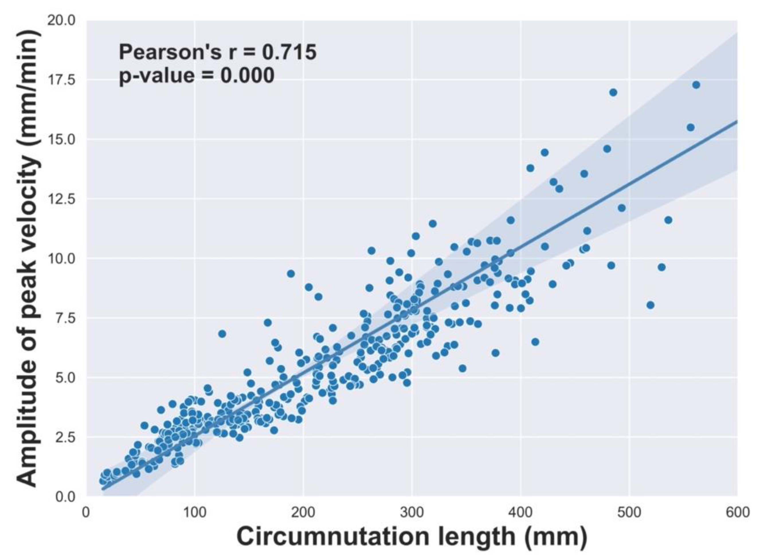
We noticed a non-significant difference for circumnutation duration across conditions while the amplitude of peak velocity increased for the DS with respect to the SS condition. We felt that this may indicate the put in place of a sort of isochrony principle [16] by the plants (see Discussion section). To test this, we performed Pearson’s correlation analysis [17] between circumnutation length and the amplitude of peak velocity [18]. The results indicate a significant correlation between these measures (Pearson’s r = 0.715, p-value = .000, 95% CI: [0.663, 0.760]; Figure 2)

3. Discussion

In the current study, we examined the behavior of pea plants raised in the presence of either a single support or two supports differing in size. The results suggest that their kinematical patterning differs depending on whether they are exposed to either one or two potential supports. And that when they are put in the position to choose between a thin or a thick support, they manifest a clear preference for the former. These findings support Darwin’s [4] and others’ [3,11,19] observations suggesting that when support diameter increases beyond a certain point, climbing plants are unable to maintain tensional forces that facilitate coiling and attachment to the support. Thus, a support with a large diameter appears to be unsuitable for coiling and climbing.
But how climbing plants do avoid an unsuitable host and choose a suitable one? A common believe is that the physiological mechanisms underlying behavioral responses in plants tend to be caused by non-integrated, local reactions [20]. As proposed by Saito, these ‘reactions’ might also be at the basis of the decision-making processes related to support diameter characterizing tendrils’ coiling [12]. In this view, changes in the coiling responses may be caused by local reactions in the tendrils. For instance, in many climbing plants, the coiling of tendrils is thought to be caused by the contraction of the gelatinous fibers (G fibers) after stimuli have been contacted [12,21]. Put simply, at the basis of climbers’ support selection there might be a passive and automatic mechanism that makes it possible to select a support with an appropriate diameter.
A point worth noting is that most studies on how climbers select a support based on diameter information focus on the final coiling response, with no or little reference to the choreography assumed by the tendrils during the approach phase [7,8,22]. To fill this gap, we have measured the kinematics of tendrils’ circumnutation from the start of their growth until they grasped the support. The emerging picture might suggest a trade-off in terms of metabolic use. Grasping a thicker support would imply the growth of longer tendrils, which in turn would be more demanding in terms of energy consumption. This metabolically based decision would also reflect on movement kinematics as the movement towards thicker supports is much slower than for thinner supports [7] and implies a great deal of on-line adjustments [6]. Therefore, a certain degree of information processing is required to integrate, interpret, and compute the relative information that determines a preference for thin supports.
These aspects are particularly evident when comparing kinematics for the one and the two supports conditions of the present study, signifying that plants can perceive their surroundings and generate circumnutation patterns accordingly. When comparing circumnutation between the thin support for the SS and the DS conditions plants move faster and execute less but larger circumnutations for the latter than for the former. This signifies that despite they are aiming at supports of a similar size, being exposed to an alternative (the thicker support for the DS condition) determines a decisional complexity that is played out in the kinematics of circumnutation. Most importantly, our findings suggest that pea plants’ movement seems planned on the basis of the isochrony principle [16]. The isochrony principle refers to a spontaneous tendency to increase the velocity of a movement depending on the linear extent of its trajectory to maintain the execution time approximately constant [23]. In our circumstances, plants maintain movement duration constant and scale velocity in order to cover longer distances as witnessed by the longer circumnutation paths. This appears to be the easiest and most readily chosen organizational option by the plant to program the circumnutational patterning when a decision based on alternatives has to be taken.
Decision-making has been customarily considered as a people-centric process [24,25], implying the making of a choice from a number of alternatives to achieve a desired result [26]. In recent years, decision-making has been studied on a variety of organisms [27], including plants [28,29]. Dener and colleagues investigated decision-making in the root development of pea plant (Pisum sativum) using the risk sensitivity theory (RST) [28]. According to RST, the rational decision is the one that maximizes fitness [30]. In the study, root growth displayed both risk-prone and risk-averse behaviors, which better support the RST hypothesis than previous animal testing. It appears that pea plants make more "rational" economic decisions than species such as birds and humans in terms of risk sensitivity [28,31]. Plant decision-making is also explored in the context of the social environment. Gruntman and colleagues compared the responses of Potentilla reptans centered on their ability to outcompete their neighbors for accessing light [29]. Observed shifts in the responses between vertical growth, shade tolerance, and lateral growth suggest that plants can choose adaptively from several alternatives under light-competition scenarios [29].
Altogether, these findings suggest that plants possess the ability to make decisions and adjust their behavior in response to their surroundings. Our findings add this to the literature demonstrating that plant behavior is flexible, as opposed to rigid and mechanical [32], reinforcing the idea that plants are open systems with a remarkable ability to deal with the complexities of an ever-changing environment [33].
At this stage, the natural question is how and at which level pea plants implement such decisions which translate into specific behavioral patterns. One possible mechanism could be light acquisition at the level of the stomata [34,35], which might allow them to distinguish the light reflections determined by differently sized supports. Alternatively, Souza and colleagues introduced the concept of “plant electrome” describing the totality of the ionic dynamics at different scales of plant organization, engendering a constant electrical activity [36,37]. Souza and colleagues demonstrated that, rather than pure random noise, the amount of complexity characterizing environmental stimuli might alter several characteristics of the temporal dynamics of the plant electrome [36,38,39]. It was reported that some frequencies (the higher ones) exhibited by non-stimulated plants faded after stimulation. Only the lowest frequencies remain, allowing for low-energy-cost long-distance signaling [37]. In this view, the electrome could be considered as a unifying factor of whole plant reactivity in a constantly changing environment and therefore might be a good candidate to understand the flexible behavior of plants [37].
In conclusion, the results of this study offer a contextual framework for the different well-known responses of climbing plants when searching for a support. More importantly, we have demonstrated a decision-making ability in plants, which allows them to adaptively ‘choose’ between responses, according to the relative structure of available supports. Overall, the results of our study suggest that plants are capable of acquiring and integrating complex information about their environment in order to adaptively modify their extent of plastic responses. Such complex decision-making in plants could have important implications for our understanding of the processes that govern plant behavior. And open to the possibility that plants may deploy a higher level of ‘cognitive’ complexity than previously thought, providing further evidence against traditional views considering plants as passive organisms.

4. Materials and Methods

4.1. Subjects

16 snow peas (Pisum Sativum var. Saccharum cv Carouby de Maussane) were chosen as study plants. Seeds were potted at 8 cm from the pot’s border and sowed at a depth of 2.5 cm.

4.2. Type of support

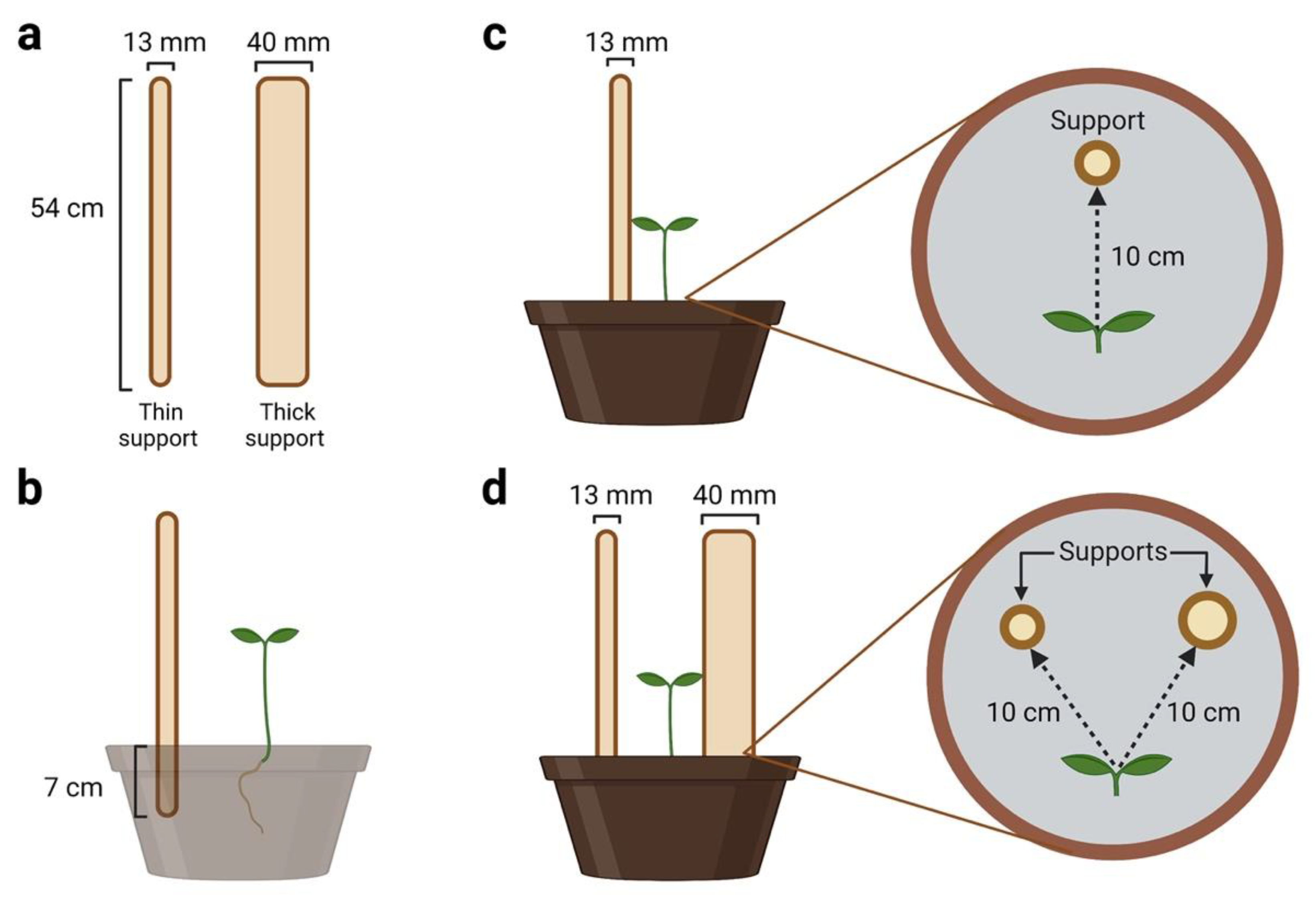
Two types of wooden support were considered: a ‘thin’ support of 13 mm in diameter (Koto -13 mm) and a ‘thick’ support of 40 mm in diameter (Koto - 40 mm; Figure 3a). Both supports were 54 cm in height. The supports were inserted 7 cm below the soil surface (Figure 3b).

4.3. Experimental conditions

The subjects were randomly assigned to two experimental conditions termed single (SS) and double support (DS) conditions. For the SS condition, 8 plants were raised individually in the presence of the ‘thin’ support (Figure 3c). For the DS condition (Figure 3d), 8 plants were raised individually in the presence of both the ‘thin’ and the ‘thick’ support. The location of the differently sized supports was counterbalanced across subjects to avoid a potential bias due to the direction of circumnutation (clockwise or counterclockwise). The supports were positioned so that the first leaf developed by a sprout faced the midpoint between the two supports. This was done to prevent a growing bias in favor of either one or the other support.

4.4. Experimental setup

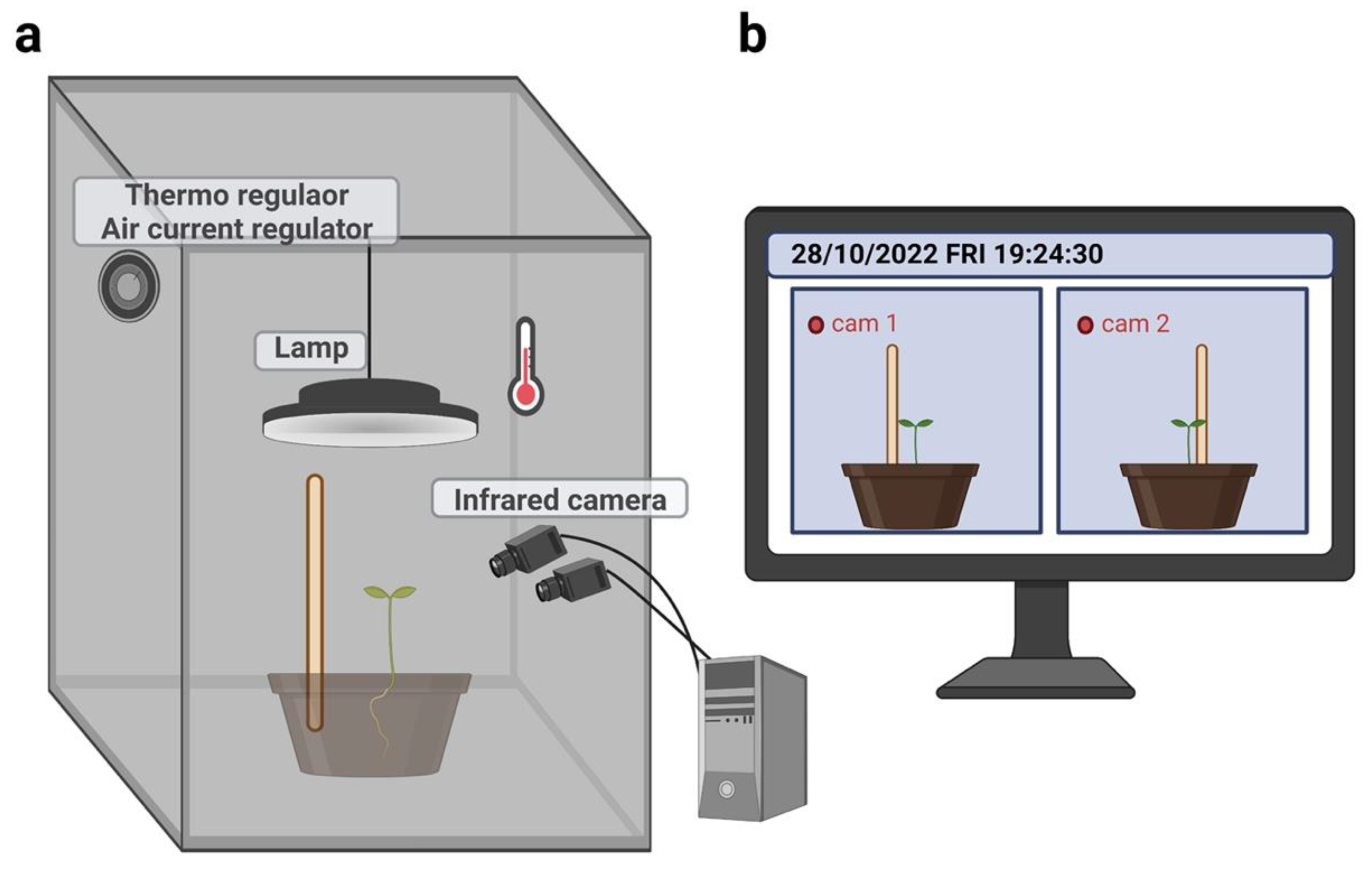
Plants grew individually in a thermo-light-controlled growth chamber (Cultibox SG combi 80×80×160 cm; Figure 4). The temperature was set at 26 °C by means of an extractor fan equipped with a thermo-regulator (TT125 vents; 125 mm-diameter; max 280 mc/h) and an input-ventilation fan (Blauberg Tubo 100 - 102 m3/h). The two-fan combination allowed for a steady air flow rate into the growth chamber with a mean air residence time of 60 seconds. The fan was carefully placed so that air circulation did not affect the plants’ movements. Cylindrical pots (40cm in diameter, 20cm in depth) were filled with river sand (type 16SS, dimension 0.8/1.2 mm, weight 1.4) and positioned at the center of the growth chamber. Each plant was exposed for 12 hours (6 a.m. to 6 p.m.) to a cool white led lamp (V-TAC innovative LED lighting, VT-911-100W, Des Moines, IA, USA) that was positioned 50 cm above each seedling. Photosynthetic Photon Flux Density at 50 cm under the lamp in correspondence with the seedling was 350 µmolph/(m2s) (quantum sensor LI-190R, Lincoln, Nebraska, USA). At the beginning of each experiment, the pots were fertilized using a half-strength solution culture (Murashige and Skoog Basal Salt Micronutrient Solution; see components & organics). The pots were watered three times a week using distilled water (Sai Acqua Demineralizzata, Parma, Italy).

4.5. Kinematic acquisition and data processing

For each growth chamber, a pair of RGB-infrared cameras (IP 2.1 Mpx outdoor varifocal IR 1080P) were placed 110 cm above the ground, spaced at 45 cm to record stereo images of the plant (Figure 4). The cameras were connected via Ethernet cables to a 10-port wireless router (D-link Dsr-250n) connected via Wi-Fi to a PC. The frame acquisition and saving process were controlled by CamRecorder software (Ab.Acus s.r.l., Milan, Italy; Figure 4). Each camera’s intrinsic, extrinsic, and lens distortion parameters were estimated using a Matlab Camera Calibrator App. Depth extraction from the single images was carried out by taking 20 pictures of a chessboard (squares’ size 18×18 mm, 10 columns × 7 rows) from multiple angles and distances in natural non-direct light conditions. For stereo calibration, the same chessboard used for the single-camera calibration process was placed in the middle of the growth chamber. The two cameras synchronously acquired the frame every 180 seconds (frequency 0.0056 Hz). RGB images were acquired during the daylight cycle and infrared images during the night cycle. The anatomical landmarks of interest were the tendrils developing from the considered leaf. We considered the initial frame as the one corresponding to the appearance of the tendrils for the considered leaf. The end frame was defined as the frame in which the tendrils start to coil the support. Images from both left and right cameras were used in order to reconstruct 3D trajectories. An ad hoc software (Ab.Acus s.r.l., Milan, Italy) developed in Matlab was used to identify anatomical points to be investigated by means of markers, and to track their position frame-by-frame on the images acquired by the two cameras to reconstruct the 3D trajectory of each marker. The markers on the anatomical landmarks of interest (i.e., the tendrils) were inserted post-hoc. The tracking procedures were at first performed automatically throughout the time course of the movement sequence using the Kanade-Lucas-Tomasi (KLT) algorithm on the frames acquired by each camera, after distortion removal. The tracking was manually verified by the experimenter, who checked the position of the markers frame-by-frame. The 3-D trajectory of each tracked marker was computed by triangulating the 2-D trajectories obtained from the two cameras. Finally, the trajectory was reconstructed with a series of coordinates in 3D (x, y, z), where the x-z plane is the horizontal plane, and the x-y plane and z-y plane as the vertical planes perpendicular to each other.

4.6. Dependent measure

The considered dependent measures were the following [40]:
(i)
Number of circumnutations: the number of circumnutations performed by a plant from the time it was potted to the time it grasped the support.
(ii)
Circumnutation duration: the time taken by a plant to complete a single circumnutation.
(iii)
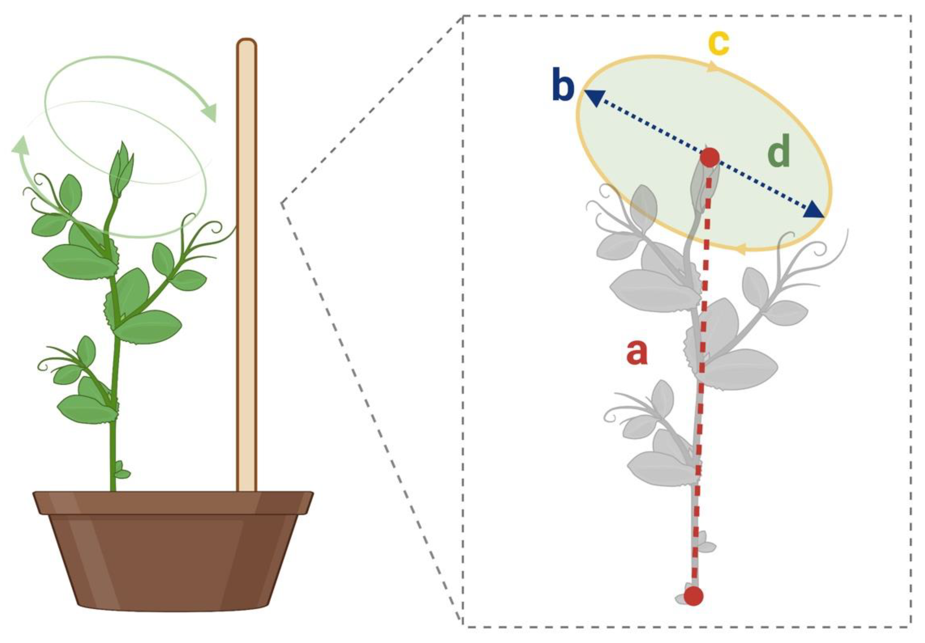
Distance from the center of circumnutation to the origin (Figure 5. segment a): The distance between the circumnutation center and the plant origin.
(iv)
Length of the circumnutation major axis (Figure 5. segment b): the maximum distance between two points of the circumnutation trajectory.
(v)
Circumnutation length (Figure 5. segment c): the length of the overall path computed as the sum of all the Euclidean distances between subsequent points during a single circumnutation.
(vi)
Circumnutation area (Figure 5. segment d): the sum of pixels with a value equal to 1 obtained from the binarization of the circumnutation trajectory.
(vii)
Amplitude of peak velocity: values for the average of maximum velocity.

4.7. Statistical analysis

The descriptive statistics including mean, standard deviation (SD), standard error (SE), and coefficient of variation have been calculated. Statistical analyses were conducted using the Bayesian approach. The objective of Bayesian estimation is to allocate credibility to a distribution of alternative parameter values (posterior distribution) that is consistent with the observed data, by generating a large number of samples using the Markov chain Monte Carlo approach (MCMC). In this study, we adopt the two-sided Bayesian Mann-Whitney U test since the dependent variables are not normally distributed. Mann-Whitney U test is a non-parametric test that does not require the assumption of normality. The analysis was performed using JASP [41] nested within the environment R (see used packages) [42]. We choose the default prior defined by a Cauchy distribution centered on a zero-effect size (δ) and a scale of 0.707 because prior knowledge regarding the exposition of plants to a double-support condition is absent [43,44]. Data augmentation is generated with 5 chains of 1000 iterations that allows for simpler and more feasible simulation from a posterior distribution. In the analysis, W is calculated in the Mann-Whitney U test as the smaller of the rank total between the two conditions. Bayes factor (BF) is obtained to quantify the relative predictive performance of two hypotheses [43]. In our study, BF quantifies evidence for the presence or absence of the difference between the DS condition and the SS condition. The null hypothesis (H0) here is that there is no difference in kinematics between the DS and the SS condition. The alternative hypothesis (H1) is that there is a difference. The BF10 value is the likelihood given H1 divided by H0. The BF01 value is calculated as H0 divided by H1. The results are reported based on Jeffery’s scheme that proposes a series of labels for which specific Bayes factor values can be considered either “no evidence”, “anecdotal (1 – 3)”, “moderate (3 – 10)”, “strong (10 – 30)”, “very strong (30 – 100)”, or “decisive (> 100)” relative evidence for alternative hypothesis [45]. R-hat is also reported to check the degree of convergence of MCMC algorithms based on outcomes stability. The closer the value of R-hat is to 1, the better convergence to the underlying distribution. Credible intervals (CI) are set as 95%, which is simply the central portion of the posterior distribution that contains 95% of the values.

Author Contributions

Conceptualization, Q.W. and U.C.; methodology, Q.W.; software, Q.W. and V.S.; validation, Q.W.; formal analysis, Q.W.; investigation, Q.W., S.G and B.B.; resources, M.B.; data curation, Q.W.; writing—original draft preparation, Q.W. and U.C.; writing—review and editing, U.C. and Q.W.; visualization, Q.W.; supervision, U.C.; project administration, Q.W. All authors have read and agreed to the published version of the manuscript.

Funding

This research received no external funding.

Data Availability Statement

The data is available online.

Acknowledgments

Figures 3-5 were created with BioRender.com. Qiuran Wang is funded by the China Scholarship Council (CSC). We thank Matthew Sims for the invaluable comments to this research project.

Conflicts of Interest

The authors declare no conflict of interest.

References

  1. Niklas, K.J. Climbing plants: attachment and the ascent for light. Current Biology 2011, 21, R199–R201. [Google Scholar] [CrossRef]
  2. Gianoli, E. The behavioural ecology of climbing plants. AoB Plants 2015, 7. [Google Scholar] [CrossRef]
  3. Gianoli, E.; Gonzalez-Teuber, M. Effect of support availability, mother plant genotype and maternal support environment on the twining vine Ipomoea purpurea. Plant Ecology 2005, 179, 231–235. [Google Scholar] [CrossRef]
  4. Darwin, C. The movements and habits of climbing plants; John Murray: London, UK, 1875. [Google Scholar]
  5. Ceccarini, F.; Guerra, S.; Peressotti, A.; Peressotti, F.; Bulgheroni, M.; Baccinelli, W.; Bonato, B.; Castiello, U. Speed–accuracy trade-off in plants. Psychonomic Bulletin & Review 2020, 27, 966–973. [Google Scholar]
  6. Ceccarini, F.; Guerra, S.; Peressotti, A.; Peressotti, F.; Bulgheroni, M.; Baccinelli, W.; Bonato, B.; Castiello, U. On-line control of movement in plants. Biochemical and Biophysical Research Communications 2020. [CrossRef]
  7. Guerra, S.; Peressotti, A.; Peressotti, F.; Bulgheroni, M.; Baccinelli, W.; D’Amico, E.; Gomez, A.; Massaccesi, S.; Ceccarini, F.; Castiello, U. Flexible control of movement in plants. Sci Rep 2019, 9, 16570. [Google Scholar] [CrossRef]
  8. Guerra, S.; Bonato, B.; Wang, Q.; Peressotti, A.; Peressotti, F.; Baccinelli, W.; Bulgheroni, M.; Castiello, U. Kinematic Evidence of Root-to-Shoot Signaling for the Coding of Support Thickness in Pea Plants. Biology 2022, 11, 405. [Google Scholar] [CrossRef]
  9. Castiello, U. (Re) claiming plants in comparative psychology. Journal of Comparative Psychology 2020, 135, 127–141. [Google Scholar] [CrossRef]
  10. Carrasco-Urra, F.; Gianoli, E. Abundance of climbing plants in a southern temperate rain forest: host tree characteristics or light availability? Journal of Vegetation Science 2009, 20, 1155–1162. [Google Scholar] [CrossRef]
  11. Goriely, A.; Neukirch, S. Mechanics of climbing and attachment in twining plants. Physical Review Letters 2006, 97, 184302. [Google Scholar] [CrossRef]
  12. Saito, K. A study on diameter-dependent support selection of the tendrils of Cayratia japonica. Sci Rep 2022, 12, 1–8. [Google Scholar] [CrossRef]
  13. Putz, F.E.; Holbrook, N.M. Biomechanical studies of vines. The Biology of Vines 1992, 73–98. [Google Scholar]
  14. Rowe, N.P.; Isnard, S.; Gallenmüller, F.; Speck, T. 2 Diversity of Mechanical Architectures in Climbing Plants: An Ecological Perspective. Ecology and Biomechanics: A Mechanical Approach to the Ecology of Animals and Plants 2006, 35.
  15. Sousa-Baena, M.S.; Hernandes-Lopes, J.; Van Sluys, M.-A. Reaching the top through a tortuous path: helical growth in climbing plants. Current Opinion in Plant Biology 2021, 59, 101982. [Google Scholar] [CrossRef]
  16. Viviani, P.; McCollum, G. The relation between linear extent and velocity in drawing movements. Neuroscience 1983, 10, 211–218. [Google Scholar] [CrossRef]
  17. Cohen, I.; Huang, Y.; Chen, J.; Benesty, J.; Benesty, J.; Chen, J.; Huang, Y.; Cohen, I. Pearson correlation coefficient. Noise Reduction in Speech Processing 2009, 1–4. [Google Scholar]
  18. Van Rossum, G.; Drake Jr, F.L. Python tutorial; Centrum voor Wiskunde en Informatica Amsterdam, The Netherlands: 1995; Volume 620.
  19. Putz, F.E. The natural history of lianas on Barro Colorado Island, Panama. Ecology 1984, 65, 1713–1724. [Google Scholar] [CrossRef]
  20. Karban, R. Plant behaviour and communication. Ecology Letters 2008, 11, 727–739. [Google Scholar] [CrossRef]
  21. Bowling, A.J.; Vaughn, K.C. Gelatinous fibers are widespread in coiling tendrils and twining vines. American Journal of Botany 2009, 96, 719–727. [Google Scholar] [CrossRef]
  22. Guerra, S.; Bonato, B.; Wang, Q.; Ceccarini, F.; Peressotti, A.; Peressotti, F.; Baccinelli, W.; Bulgheroni, M.; Castiello, U. The coding of object thickness in plants: When roots matter. Journal of Comparative Psychology 2021. [CrossRef]
  23. Sartori, L.; Camperio-Ciani, A.; Bulgheroni, M.; Castiello, U. Reach-to-grasp movements in Macaca fascicularis monkeys: the Isochrony Principle at work. Frontiers in Psychology 2013, 4, 114. [Google Scholar] [CrossRef]
  24. Svenson, O. Process descriptions of decision making. Organizational Behavior and Human Performance 1979, 23, 86–112. [Google Scholar] [CrossRef]
  25. Lunenburg, F.C. The decision making process. In Proceedings of the National Forum of Educational Administration & Supervision Journal; 2010. [Google Scholar]
  26. Eisenfuhr, F. Decision making. Academy of Management Review 2011, 19, 312–330. [Google Scholar]
  27. Kacelnik, A.; El Mouden, C. Triumphs and trials of the risk paradigm. Animal Behaviour 2013, 86, 1117–1129. [Google Scholar] [CrossRef]
  28. Dener, E.; Kacelnik, A.; Shemesh, H. Pea plants show risk sensitivity. Current Biology 2016, 26, 1763–1767. [Google Scholar] [CrossRef]
  29. Gruntman, M.; Groß, D.; Májeková, M.; Tielbörger, K. Decision-making in plants under competition. Nature Communications 2017, 8, 2235. [Google Scholar] [CrossRef]
  30. McNamara, J.M.; Houston, A.I. Risk-sensitive foraging: a review of the theory. Bulletin of Mathematical Biology 1992, 54, 355–378. [Google Scholar] [CrossRef]
  31. Schmid, B. Decision-making: are plants more rational than animals? Current Biology 2016, 26, R675–R678. [Google Scholar] [CrossRef]
  32. Calvo, P. The philosophy of plant neurobiology: a manifesto. Synthese 2016, 193, 1323–1343. [Google Scholar] [CrossRef]
  33. Souza, G.M.; Toledo, G.R.; Saraiva, G.F. Towards systemic view for plant learning: ecophysiological perspective. Memory and Learning in Plants 2018, 163–189. [Google Scholar]
  34. Chen, C.; Xiao, Y.-G.; Li, X.; Ni, M. Light-regulated stomatal aperture in Arabidopsis. Molecular Plant 2012, 5, 566–572. [Google Scholar] [CrossRef]
  35. Sharkey, T.D.; Raschke, K. Separation and measurement of direct and indirect effects of light on stomata. Plant Physiology 1981, 68, 33–40. [Google Scholar] [CrossRef]
  36. Souza, G.M.; Ferreira, A.S.; Saraiva, G.F.; Toledo, G.R. Plant “electrome” can be pushed toward a self-organized critical state by external cues: Evidences from a study with soybean seedlings subject to different environmental conditions. Plant Signaling & Behavior 2017, 12, e1290040. [Google Scholar]
  37. Debono, M.W.; Souza, G.M. Plants as electromic plastic interfaces: A mesological approach. Progress in Biophysics and Molecular Biology 2019, 146, 123–133. [Google Scholar] [CrossRef]
  38. Saraiva, G.; Ferreira, A.; Souza, G. Osmotic stress decreases complexity underlying the electrophysiological dynamic in soybean. Plant Biology 2017, 19, 702–708. [Google Scholar] [CrossRef]
  39. Bak, P.; Tang, C.; Wiesenfeld, K. Self-organized criticality: An explanation of the 1/f noise. Physical Review Letters 1987, 59, 381. [Google Scholar] [CrossRef]
  40. Simonetti, V.; Bulgheroni, M.; Guerra, S.; Peressotti, A.; Peressotti, F.; Baccinelli, W.; Ceccarini, F.; Bonato, B.; Wang, Q.; Castiello, U. Can Plants Move Like Animals? A Three-Dimensional Stereovision Analysis of Movement in Plants. Animals 2021, 11, 1854. [Google Scholar] [CrossRef]
  41. JASP Team, JASP (Version 0.17) [Computer software], 2023.
  42. R Development Core Team, R: A language and environment for statistical computing, R Foundation for Satistical Computing: 2010.
  43. van Doorn, J.; van den Bergh, D.; Böhm, U.; Dablander, F.; Derks, K.; Draws, T.; Etz, A.; Evans, N.J.; Gronau, Q.F.; Haaf, J.M. The JASP guidelines for conducting and reporting a Bayesian analysis. Psychonomic Bulletin & Review 2021, 28, 813–826. [Google Scholar]
  44. Ly, A.; Verhagen, J.; Wagenmakers, E.-J. Harold Jeffreys’s default Bayes factor hypothesis tests: Explanation, extension, and application in psychology. Journal of Mathematical Psychology 2016, 72, 19–32. [Google Scholar] [CrossRef]
  45. Jeffreys, H. The theory of probability; OuP Oxford: New York, NY, USA, 1998. [Google Scholar]
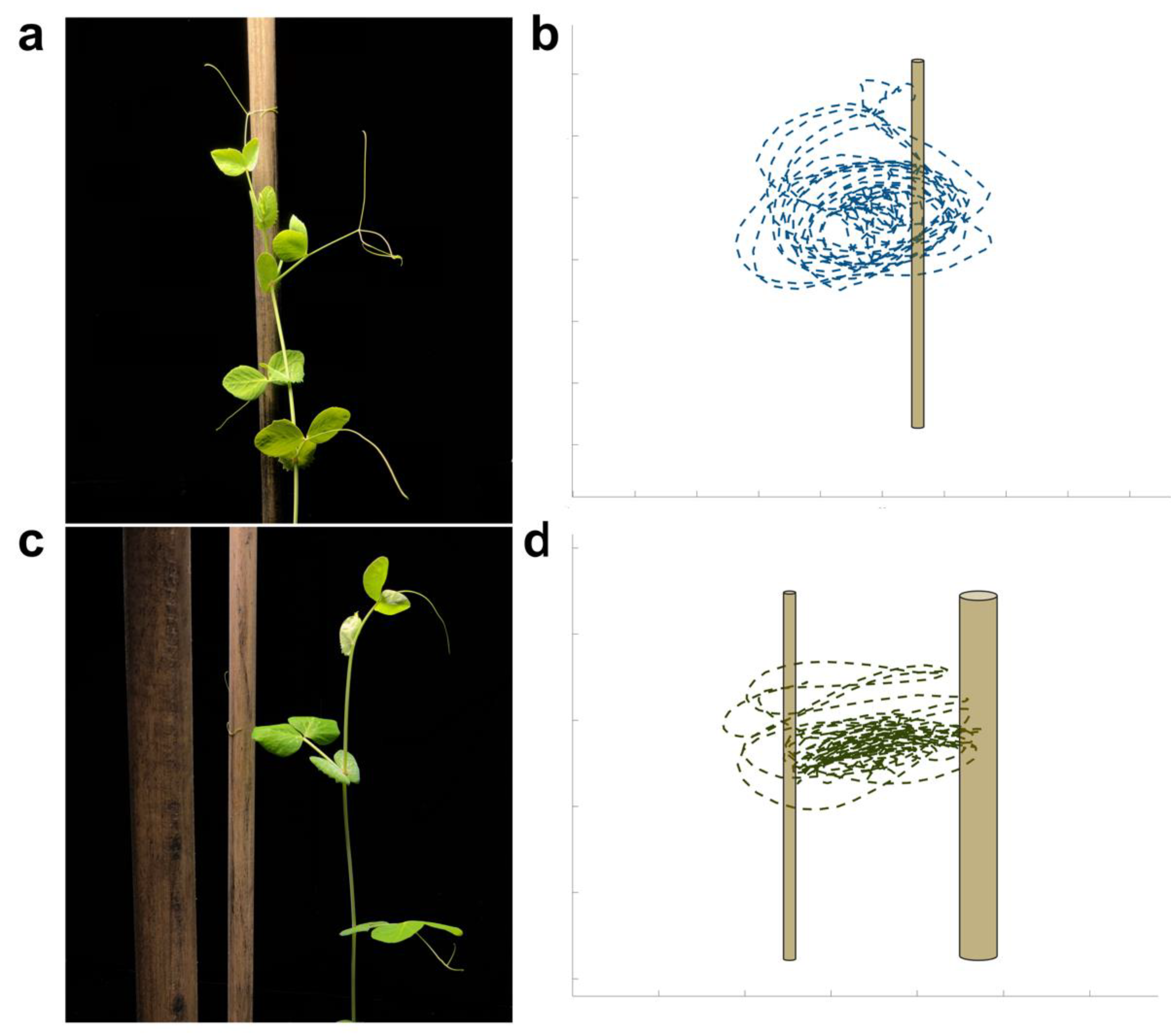
Figure 1. (a) A frame representing an exemplar plant grasping the support for the single-support (SS) condition and the graphical representation of its trajectory (b). (c) A plant grasping the thinner support for the double-support (DS) condition and the graphical representation of its trajectory (d).
Preprints 69251 g001
Figure 2. Pearson’s correlation coefficient between the “circumnutation length” and the “amplitude of peak velocity”.
Preprints 69251 g002
Figure 3. (a)Graphical depiction of the “thin” and the “thick” support; (b) the location of the support in the pot, and how it was inserted in the soil. The single-support and the double-support condition are represented in panels c and d, respectively.
Preprints 69251 g003
Figure 4. Graphical illustration of the experimental setup (a). Panel b represents how the plants were ‘seen’ by the infrared cameras.
Preprints 69251 g004
Figure 5. Graphical representation for some of the considered dependent measure. (a) The distance from the center of circumnutation to the origin is represented as red/dash line; (b) the length of the circumnutation major axis is represented as blue/dash line; (c) the circumnutation length is represented as yellow/solid line; (d) the circumnutation area is represented in green.
Preprints 69251 g005
Table 1. Descriptive statistics for the considered dependent measures.
95% CI
Group Mean SD SE Coefficient
of variation
Lower Upper
Number of circumnutations DS 24.924 4.247 0.303 0.170 24.327 25.521
SS 26.553 6.156 0.439 0.232 25.688 27.418
Circumnutation duration (min)
DS 66.746 13.190 0.940 0.198 64.893 68.600
SS 69.000 14.451 1.030 0.209 66.969 71.031
Distance from the circumnutation center to the origin (cm) DS 16.004 10.145 0.723 0.634 14.579 17.430
SS 28.660 25.146 1.792 0.877 25.127 32.194
Length of the circumnutation major axis (mm)

DS 91.214 38.929 2.774 0.427 85.744 96.684
SS 72.908 43.538 3.102 0.597 66.791 79.026
Circumnutation length (mm)
DS 243.403 124.957 8.903 0.513 225.846 260.961
SS 188.148 115.972 8.263 0.616 171.853 204.443
Circumnutation area (mm2)
DS 4992.504 4634.422 330.189 0.928 4341.325 5643.684
SS 3217.099 3505.097 249.728 1.090 2724.601 3709.598
Amplitude of maximum peak velocity (mm/min)
DS 6.541 5.650 0.403 0.864 5.748 7.335
SS 4.660 2.840 0.202 0.610 4.260 5.059
Note. DS = double-support condition; SS = single-support condition; SD = standard deviation; SE = standard error; CI = credible interval
Table 2. Two-sided Bayesian Mann-Whitney U test for the DS and the SS conditions.
BF₁₀ W R-hat
Number of circumnutation 314.656 14220.000 1.008
Circumnutation duration 0.387 17083.000 1.000
Distance from the circumnutation center to the origin 43.665 15057.000 1.007
Length of the circumnutation major axis 734.705 24455.000 1.016
Circumnutation length 980.421 24433.000 1.015
Circumnutation area 1267.886 24611.500 1.008
Amplitude of maximum peak velocity 4137.588 25438.000 1.014
Note. Result based on data augmentation algorithm with 5 chains of 1000 iterations.
Disclaimer/Publisher’s Note: The statements, opinions and data contained in all publications are solely those of the individual author(s) and contributor(s) and not of MDPI and/or the editor(s). MDPI and/or the editor(s) disclaim responsibility for any injury to people or property resulting from any ideas, methods, instructions or products referred to in the content.
Copyright: This open access article is published under a Creative Commons CC BY 4.0 license, which permit the free download, distribution, and reuse, provided that the author and preprint are cited in any reuse.
Prerpints.org logo

Preprints.org is a free preprint server supported by MDPI in Basel, Switzerland.

Subscribe

© 2024 MDPI (Basel, Switzerland) unless otherwise stated