1. Introduction
1.1. Problem Statement
The ubiquitousness of sensor data in modern manufacturing is creating opportunities as well as challenges for manufactures. Since both computer-aided engineering [
1] and time series-based machine learning (ML) showed significant advancements in recent years, an increasing number of manufacturers rely on ML-based solutions to create value out of sensor data. Especially fields like predictive maintenance [
2], condition monitoring [
3], and anomaly detection [
4] have achieved immense progress and have become well-known terms in the academic and industrial world.
A less-known research area is time series segmentation (TSS), which deals with splitting up a time series into distinct non-overlapping segments. In a manufacturing setting, TSS is usually based on multivariate time series data. TSS can be utilized to detect different operational states of production machines or to recognize human actions via tracking sensors. Multivariate time series data pose special challenges for algorithms. The most successful multivariate TSS approaches proposed in recent years are based on deep learning and use a supervised learning concept (e.g., [
5]). In recent work, we analyzed a TSS use case in manufacturing and proposed a novel deep learning architecture [
6]. The presented network was successful in splitting up the end-of-line testing cycle data of hydraulic pumps into different testing phases based on nine sensor channels. However, results were based on a sufficiently large training dataset was available for each pump variant. In this paper, we build on this previous work and revisit the use case with the difference that we face training data scarcity.
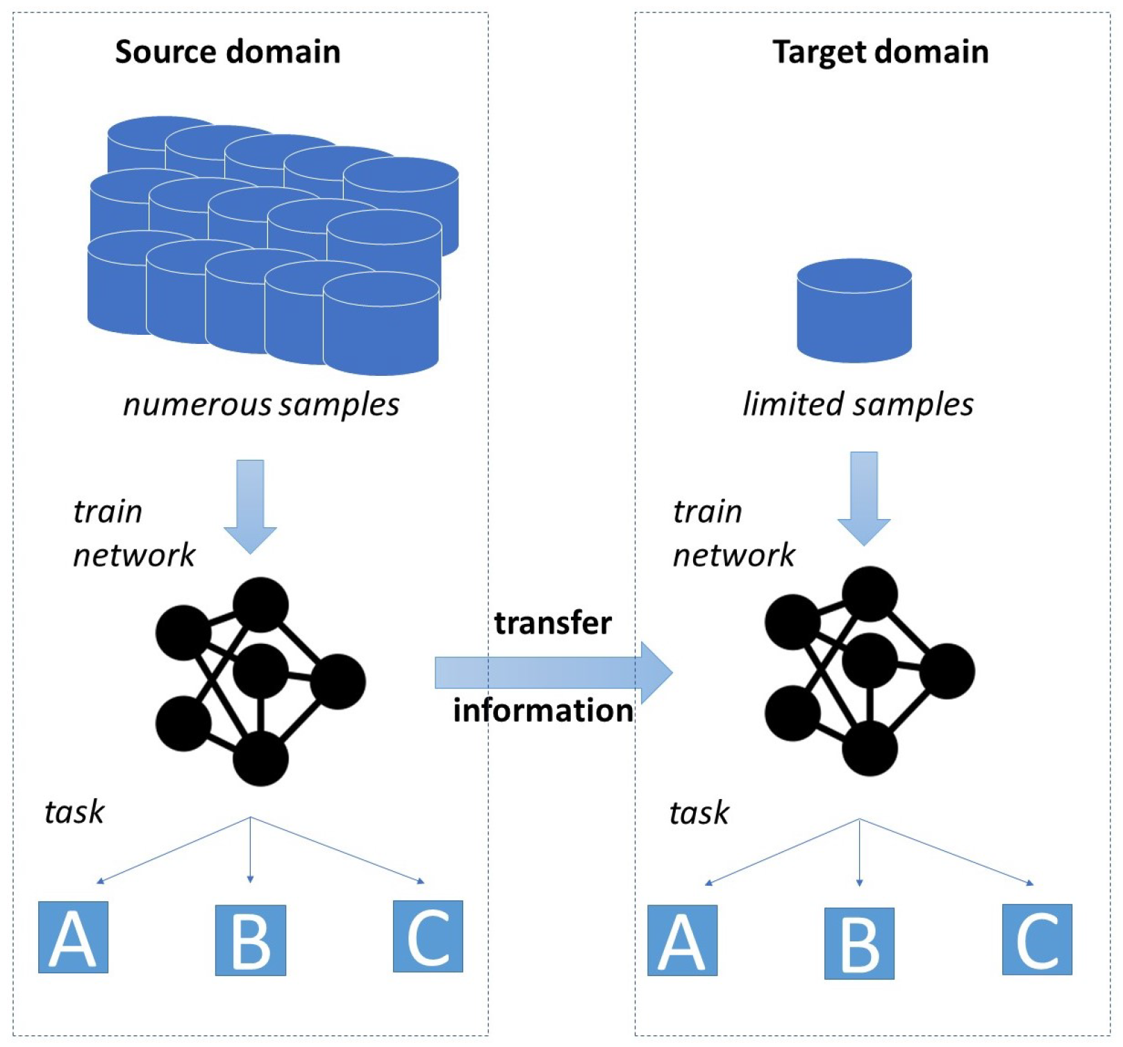
The biggest drawback of deep learning models is their heavy dependency on the availability of data. Especially, in many industrial environments the collection and labeling of required data is expensive and time consuming. In turn, there are many settings where only a limited amount of training data is available. This widespread issue of data scarcity led to the emergence of research fields that aim to find approaches being able to cope with a small amount of training data. Examples of corresponding approaches include few-shot learning, data augmentation and transfer learning (TL). The concept of TL is illustrated by
Figure 1. TL denotes the process of utilizing the information created when solving a task for solving a similar, but distinct task.
In the context of deep learning, TL describes the pretraining of the layers of a network by a
source dataset, before transferring the learned parameters to a different model, the
target model. Subsequently, the
target model is retrained by the
target dataset, which often comprises only a low number of training samples (finetuning). As basic idea the information the model learned by solving the
source problem might be helpful to boost the training process of the
target problem. Especially for production plants, TL constitutes a promising approach, as a high number of different product variants and models with widely varying quantities may be manufactured on the same shop floor. In particular, the data of products manufactured in high quantities might provide interesting information for similar goods with less turnover. This idea was recognized by many manufacturers, triggering a high number of publications in recent years about the successful use of TL in industrial settings (see exemplarily [
7,
8]). Especially in deep learning-based TSS, however, TL achieved very low attention compared to its high prevalence in other like image recognition or condition monitoring. There is close to no research on applying TL approaches to TSS settings and on analyzing what factors increase or limit the benefits of TL. One of the very few contribution covering the topic showed promising results when applying cross-domain TL to boost medical TSS, even though the scope of the analysis concerning TL is very limited [
9]. In general, no authors have ever performed a study focusing on how TL can be used to boost the performance of deep learning TSS models.
1.2. Own Contribution
With the presented problem setting and identified research gap in mind, this paper provides the following contributions:
We analyze the benefits of using TL for TSS in an industrial setting. The paper provides one of the very first works to even tackle the problem of TL for TSS in general.
We systematically analyze how pretraining with three different source datasets with varying degree of similarity to the target dataset affects the performance of the target model after finetuning.
We analyse to what degree the benefit of TL depends on the amount of available samples in the target dataset.
The use case analyzed in the paper deals with the segmentation of operational states within the end-of-line testing cycle of hydraulic pumps. This is an innovative application of time series-based deep learning for a practical manufacturing problem.
The remainder of the paper is structured as follows:
Section 2 provides an overview of related works in the area of industrial transfer learning for time series data. In
Section 3, the concept of TL, the used datasets, and the experimental designs are presented.
Section 4 describes the obtained experimental results and discusses them, followed by a conclusion and outlook in
Section 5.
2. Literature Research
Facilitated by the general breakthrough of deep learning in many domains, the related research field of TL recently got high attention and advanced significantly. Different surveys were published in recent years, providing a detailed overview of the start-of-the-art. The most extensive one focuses on the general concept of TL over all domains, including experimental results on text categorization and object detection [
10]. More recently, a systematic study was published that had focused on TL in the context of time series data, discovering that the publication frequency has sharply increased since the year 2019 [
11]. The study presented in [
12] provides a detailed summary of TL concepts, use cases, and trends in the context of industrial automation. Another field that is highly related to TL and recently got high attention is domain adaption [
13][
14]. In this paper, however, we deal with a setting that exceeds the scope of domain adaption (see
Section 3.1) and, therefore, we do not cover the various frameworks from the field. Instead we limit ourselves to review relevant contributions in two areas, namely time series-based TL and deep industrial TL. We clarify that our literature review does not cover recent contributions in the field of domain adaption
2.1. Transfer Learning for Time Series
The concept of TL has its origin in the area of image recognition. After showing promising results there, it found its way into time series-based ML. The research field is still relatively young, with most contributions being published after 2018. However, despite the novelty of the research field, time series-based TL has already been applied in various fields like manufacturing [
15], finance [
16], geoscience [
17], mobility [
18], and medicine [
19]. Successfully solved tasks include time series imaging [
20], anomaly detection [
21], classification [
22], and forecasting [
23]. A seminal work applying TL to time series classification analyzed how the pretraining of a model with a different
source datasets affects the classification accuracy of the
target task [
24]. In total, the authors tested more than 85
source datasets for pretraining and discovered that the benefit of pretraining significantly varies with the used
source dataset. While a high similarity between
source dataset and
target dataset tended to lead to performance improvement, pretraining with dissimilar datasets did not improve or even worsened the classification accuracy. Another interesting contribution demonstrates the successful application of TL to both convolutional neural networks (CNN) and long short-term-memory (LSTM) architectures when performing time series classification and time series predictions [
25].
Almost none of the previous works in the TL field focused on the task of TSS. While TSS problems might be less prevalent in everyday life of companies and researchers, they still deserve attention due to their importance for fields like human action recognition [
26], sleep staging [
5], and operational state detection [
6]. One contribution had a first look at the topic [
9] and successfully showed that feature extraction process of a TSS-CNN model can be improved when pretraining the model with a large, domain-independent
source dataset. However, a broad analysis focusing on TL as well as a detailed discussion of the implications of the results was not performed.
2.2. Deep Industrial Transfer Learning
Deep industrial transfer learning describes the concept of using formerly gained information and knowledge through deep learning to facilitate the solution of industrial problems [
27]. In industrial settings, it is often not feasible (or even not possible) to accumulate a sufficiently large amount of data required for traditional deep learning approaches. The reasons for the data scarcity include the variability and high customization of processes and products [
28], data protection regulations, and high cost of data collection, storage, and labeling [
29]. Industrial environments are highly volatile and dynamic. Wear, reconfigurations, and process adaptions [
28] often diminish the value of historical data, leading to only a limited amount of short-term data accurately representing the correct relationship between input data and label [
30]. Therefore, approaches like TL that attempt to address the issue of data scarcity have gained increasing attention in recent years.
[
15] compared different TL approaches for anomaly detection based on pump vibration data. In turn, [
31] used already outdated data for pretraining their network to boost the prediction accuracy compared to a cold-start network. Results were verified on two industrial datasets (solar, furnace). Another approach combined both few-shot learning and TL techniques to overcome the issue of a small training set in rotatory machine fault detection [
7]. [
8] used a huge general-domain dataset to train the feature extractor of a CNN, before finetuning the classificator with the small
target dataset to diagnose gear faults. [
32] analysed whether TL can help to identify bearing defects by transferring learned features across data of different working conditions. The authors could show that their proposed TL approach increases the effectiveness of vibration-based fault detection models. Staying in the area of vibration-based bearing fault detection, another contribution provided an analysis how and to what extent discriminative information found in varying settings (different sensor locations or working loads) can be transferred between networks [
33]. In turn, [
34] investigated online fault detection of pumps and motor bearing and achieved high accuracies by creating a transfer convolutional neural network compared to classic models. Finally, [
35] was able to show that the deep TL network created with a domain adaption module outperforms other approaches in a piston pump fault detection use case.
To the best of our knowledge, no other works have investigated the application of TL strategies to a TSS problem within an industrial setting. Almost all TL contributions from the time series domain focus on the tasks of forecasting, anomaly detection, and classification. There is a lack of research on TL strategies for TSS in general, and even more so for TSS use cases in industrial settings. The pump testing dataset we use in this paper was published in the context of one of our previous works [
6]. In the latter work, the dataset was used for TSS experiments in which the availability of a sufficient amount of training data was ensured. In this paper, however, we deal with data scarcity and investigate whether TL can help to facilitate the learning of the model when only few training samples are available. Thereby, we are the first to provide detailed results about the factors and conditions (sample size,
source dataset, layer freezing) that determine the benefit of TL in the context of TSS. Potential explanations on why certain conditions favor TL are discussed as well. Our findings extend previous research about time series-based TL and provide insightful implications for practical industrial use cases.
3. Experimental Design and Data
3.1. Transfer Learning Formalization
The idea of TL fundamentally differs from the traditional ML idea. Traditional ML approaches are isolation-based, meaning that they rely on an isolated dataset for the training of a distinct model in order to solve a single task. Usually, the models lack the ability to generalize well across different tasks or data. In turn, transfer learning allows incorporating previously learned knowledge from other tasks in order to avoid some of the common ML drawbacks. Usually, the transferable knowledge is more valuable if the domains of the different models are related. While TL is a broad field with a number of different approaches and concepts, this paper focuses on a specific TL setting in which both the
source domain and the
target domain have labeled data and the transfer consists of pretraining a model with a
source dataset (see
Figure 2).
In our work, we reuse the formalization introduced by [
36]. In general, a ML problem comprises two components, the domain and the task. A domain is formed by two elements, i.e., the feature space X and the probability distribution P(X). We denote a specific domain D as D=(X, P(X)). A task comprises two elements, namely the label space Y and the prediction function f(x) that is used to predict the label of a given instance x. The prediction function is learned by training the model via corresponding pairs of
and
. Moreover, function f(x) can be also interpreted as conditional probability distribution
. Thereby, a specific task is denoted as
or
.
With these definitions, transfer learning can be formalized: Assume that we have a
source domain , a
source task, a
target domain, and a
target task. TL aims to enhance finding the most accurate
target model f(x) in
by incorporating the information in
and
with either
, or
, or both. One subcategory of TL is domain adaption, which is applicable for scenarios, in which only the probability distributions
of
and
differ, while
and
are the same [
37]. However, the experimental design of our paper does not include any setting in which
source task and
target task are equivalent. In turn, domain adaption frameworks are not considered further.
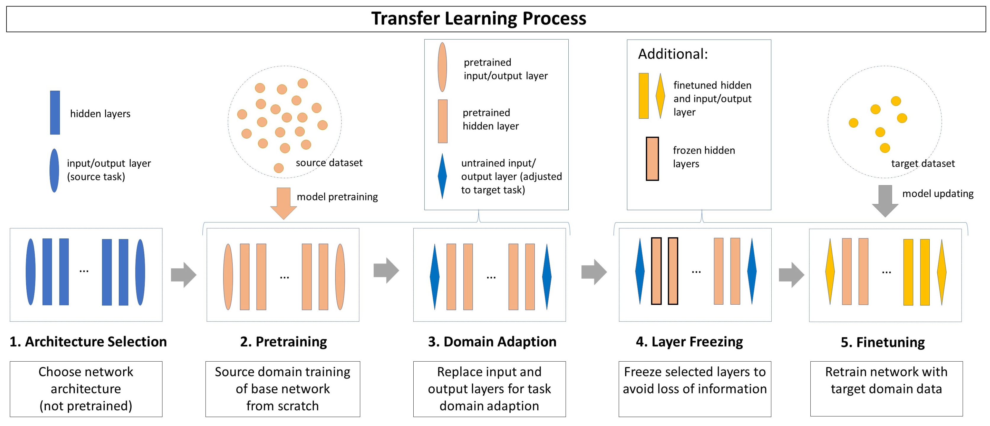
The TL approach used in this paper is illustrated in
Figure 2. It contains 5 steps:
Step 1 (Architecture Selection) An untrained network architecture is selected, whose hidden layer structure is assumed to solve both the source task and the target task. The input and output layers are chosen to fit the source task and source domain.
Step 2 (Pretraining) The network is trained with the source domain dataset on the source task. Usually, the source dataset is expected to contain a high number of samples to make the training effective.
Step 3 (Domain Adaption) The pretrained network is adapted to the target domain and target task, whereat the knowledge found in its hidden layers is preserved. To achieve this, only the input and output layers are replaced by untrained layers adapting the network to the target task and target domain.
Step 4 (Layer Freezing) Depending on the TL strategy, some or all hidden layers can be frozen before training for the target task. The parameters of a frozen layer are not updated in future training processes, which ensures that the knowledge learned during source domain training is preserved. As drawback, the adaption ability to the target domain data is limited.
Step 5 (Finetuning) The network is retrained on the target task with the target domain dataset. Usually, the target dataset has only a limited number of instances. The resulting model includes information from both the source domain and the target domain.
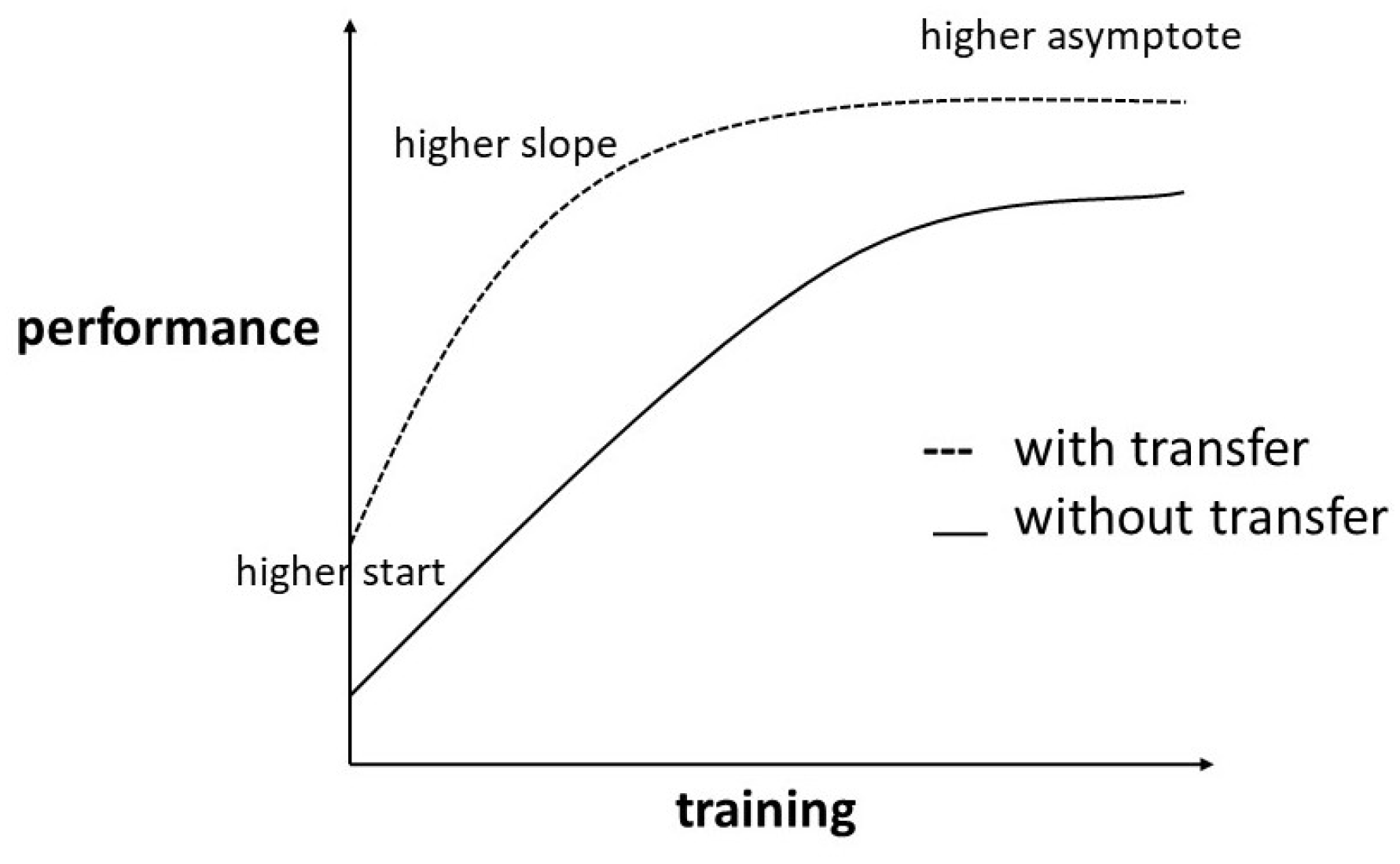
The potential advantages of TL are illustrated by
Figure 3. First, we obtain a better starting point for the model training compared to a cold start. This can be observed most often when
source domain and
target domain are heavily related and part of the learned knowledge is directly applicable to the
target task. Second, a higher slope (faster learning process) can be achieved as the result of pretraining the hidden layers. By pretraining, parameters are often set in a generally functional way and just have to be finetuned for the new task. The most important advantage for industrial use cases is the higher asymptote, meaning a higher accuracy of the final model. This can often be observed in cases where the
target dataset is very small and a part of the lacking information in the
target dataset can be filled by knowledge learned during the
source domain training. We will observe which of the three benefits can be found in the different experimental settings we describe.
In this paper, we aim to analyze how pretraining with different source datasets affects the performance of the target model. To enable a high comparability, the selected target dataset and target task stay constant across all experiments. We define three different settings:
Setting 1:Target domain and source domain share the same feature space X, and target task and source task share the same label space Y. However, the domains differ in terms of probability distribution P(X) of the feature space, while the tasks differ in the feature-label relationship (conditional probability ).
Setting 2: In addition to non-identical probability distributions P(X) and non-identical conditional probabilities , the label spaces Y of the source task and the target task differ as well. Only the feature space X of both domains is identical in this setting.
Setting 3: All four elements (feature space X, label space Y, feature probability distribution P(X),and conditional probability ) differ between source domain and target domain as well as source task and target task.
3.2. Overview on Used Datasets
In the experiments, two datasets from two different domains were used, namely (1) the Hydraulic Pump End-of-Line Dataset (HPEoL) and (2) the Opportunity Dataset.
(1) Hydraulic Pump End-of-Line Dataset
The Hydraulic Pump End-of-Line dataset collection was published recently. End-of-line testing is a type of manufacturing quality assurance process that is conducted at the end of the production line. It is used to ensure that the product meets the required specifications and that it is free from defects. In hydraulic pump testing, end-of-line testing usually consists of mounting the pump at a testbench and forcing it through a predefined testing cycle to check its function. The HPEoL dataset contains the end-of-line testing cycle data of around 198 hydraulic pumps measured by hydraulic and mechanical sensors on a hydraulic testbench. The dataset includes the testing cycle data of three different hydraulic pump types:
Direct control pumps (DC): 120 instances distributed over three versions (V35, V36, V38) differing in size and technical specifications with 40 instances each.
Speed-based (mechanical) control pumps (SC): 38 instances
Proportional control pumps (PC): 40 instances
For all control types, each sample corresponds to a multivariate time series with nine sensors representing the testing cycle of one specific pump. All 198 time series are multi-phased, meaning that each sample can be segmented into different segments representing the different testing phases of the testing cycle. While all phases of the testing cycle have to be completed for each pump, variations in the order of the phases and repetitions of phases are common. The data were collected with a frequency of 100 Hz. One testing cycle lasts between 3 and 7 minutes. Each time stamp has a integer-encoded state label representing the current testing phase of the pump at the time the sensor measures were taken. Supervised time series segmentation aims now to identify the different testing phases within the testing cycle by assigning state labels to all time stamps. Note that the testing cycles of the three different pump control types vary heavily (different label space Y), while the phases of different pump versions within a control type are very similar and only differ in the exact specification of a testing phase (identical label space Y, different conditional probabilities
). The number of different state labels for DC-types corresponds to 44, of PC-types to 43, and of SC-types to 44.
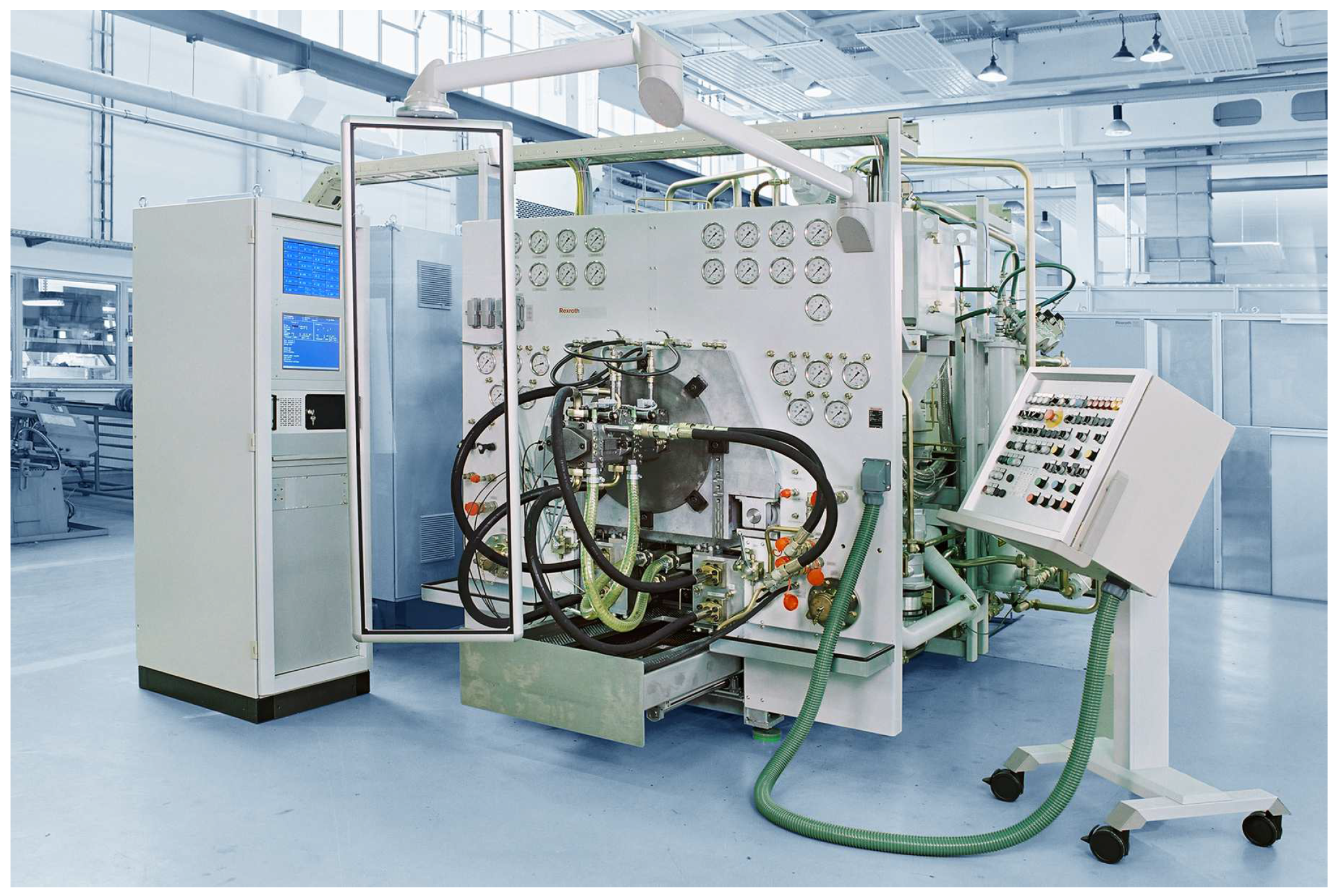
Figure 4 depicts a hydraulic testbench.
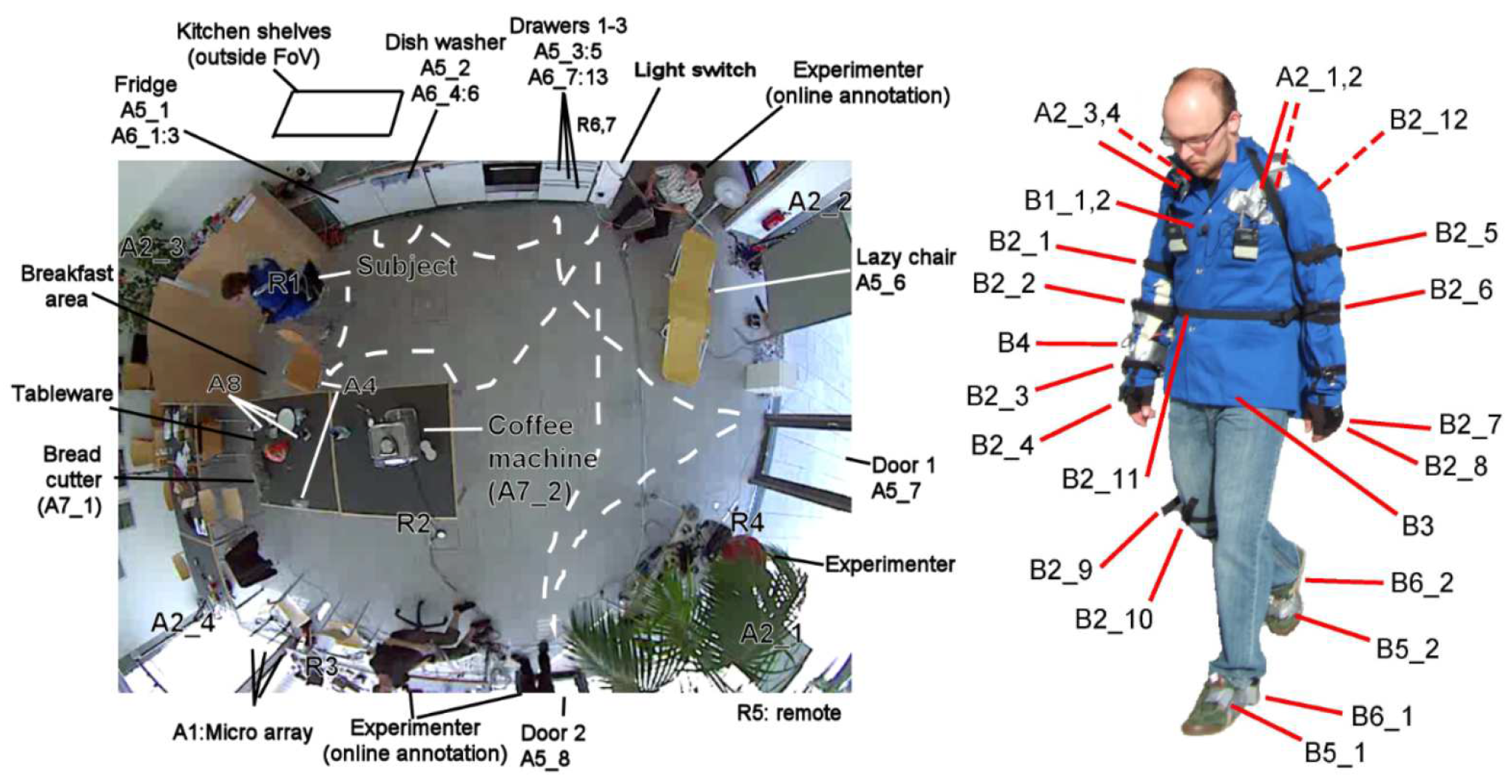
(2) Opportunity Dataset
The Opportunity dataset was published to examine and compare human activity recognition algorithms, including TSS. It includes sequences created by tracking a number of human subjects via body-worn, object-attached, and ambient sensors (like accelerometers or location sensors). The sequences are annotated by activity labels. It is a popular and widely used dataset in literature (e.g. [
26,
38] ), which has often been used for benchmarking time series-based approaches. The dataset can be structured into two parts, i.e., the ADL (Activities of Daily Life) section and the Drill section. The ADL section just follows the subjects accomplishing daily live activities (including relaxing and eating) and, in turn, has often longer time periods without a change in the activity label. In the Drill section, however, the subjects were told to perform several short activities (e.g., open doors) without any breaks in between. The activity labels, therefore, are rapidly changing, resulting in a setting that is more similar to the HPEoL dataset, in which many label switches are present within a short period of time.
Figure 5 shows the location of different sensors during the data collection process.
3.3. Model Architecture
All
source tasks and
target tasks investigated in this paper belong the category of supervised TSS tasks. More precisely, we target to find and train a deep learning model to enable it predicting the state labels for all timestamps of a multivariate time series. This is called dense labeling. The network architecture we use to analyze the impact of TL in this work is called PrecTime. The PrecTime architecture was introduced 2022 in one of our previous works [
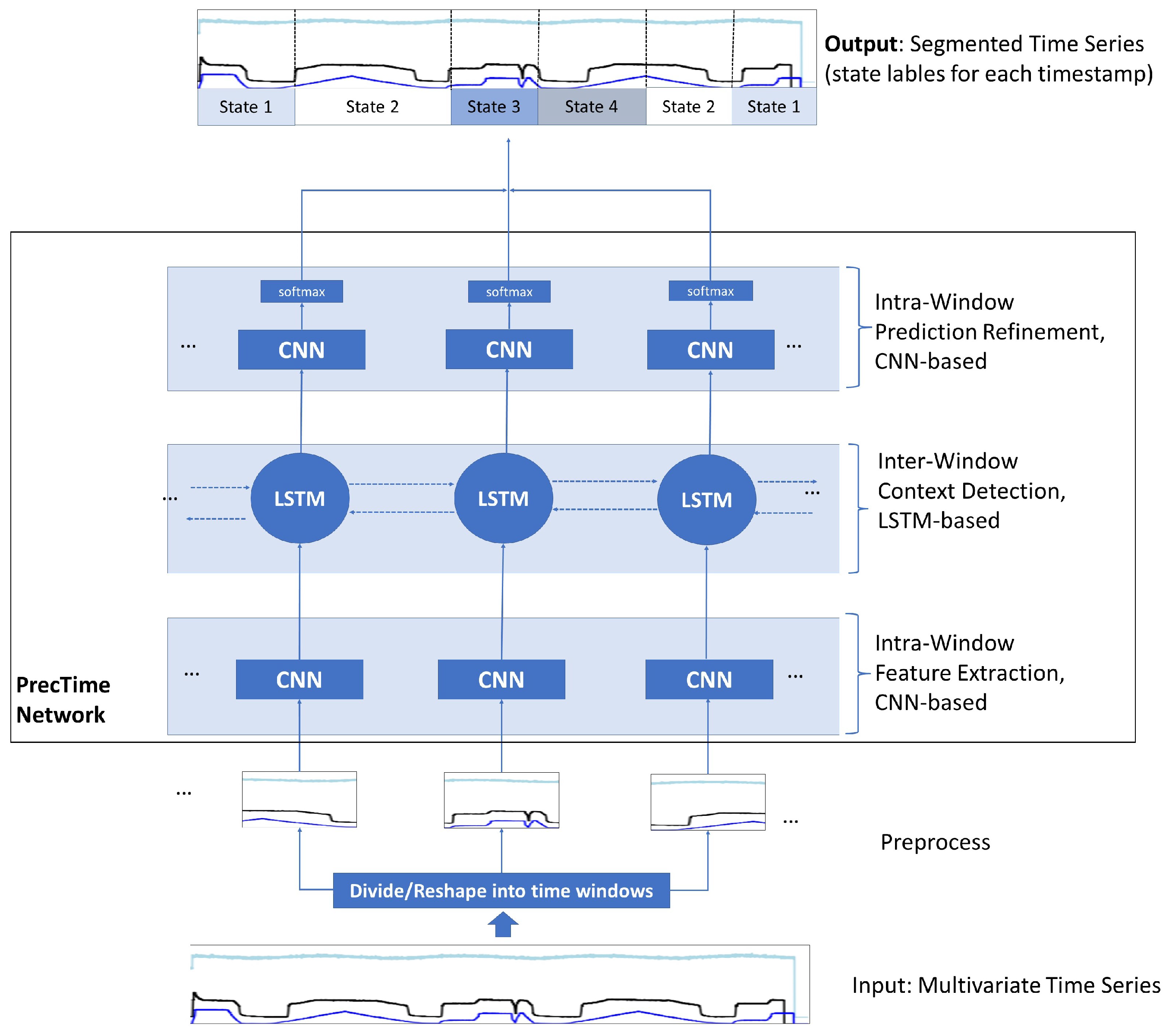
6]. It is designed for multivariate TSS and was already successfully applied to the HPEoL dataset and Opportunity dataset in isolation. As the output of the network is a sequence of state label predictions (one per time stamp), it is considered as a sequence-to-sequence model. The conceptual back bone of the network is illustrated in
Figure 6. PrecTime is a time window-based architecture consisting of three modules, i.e., a CNN-based intra-window feature extractor, an LSTM-based inter-window context detection, and an CNN-based intra-window prediction refinement model. The concrete details about the architecture, implementation, loss functions, and hyperparameters are described in [
6]. They were reused in this paper.
3.4. Experimental Setup
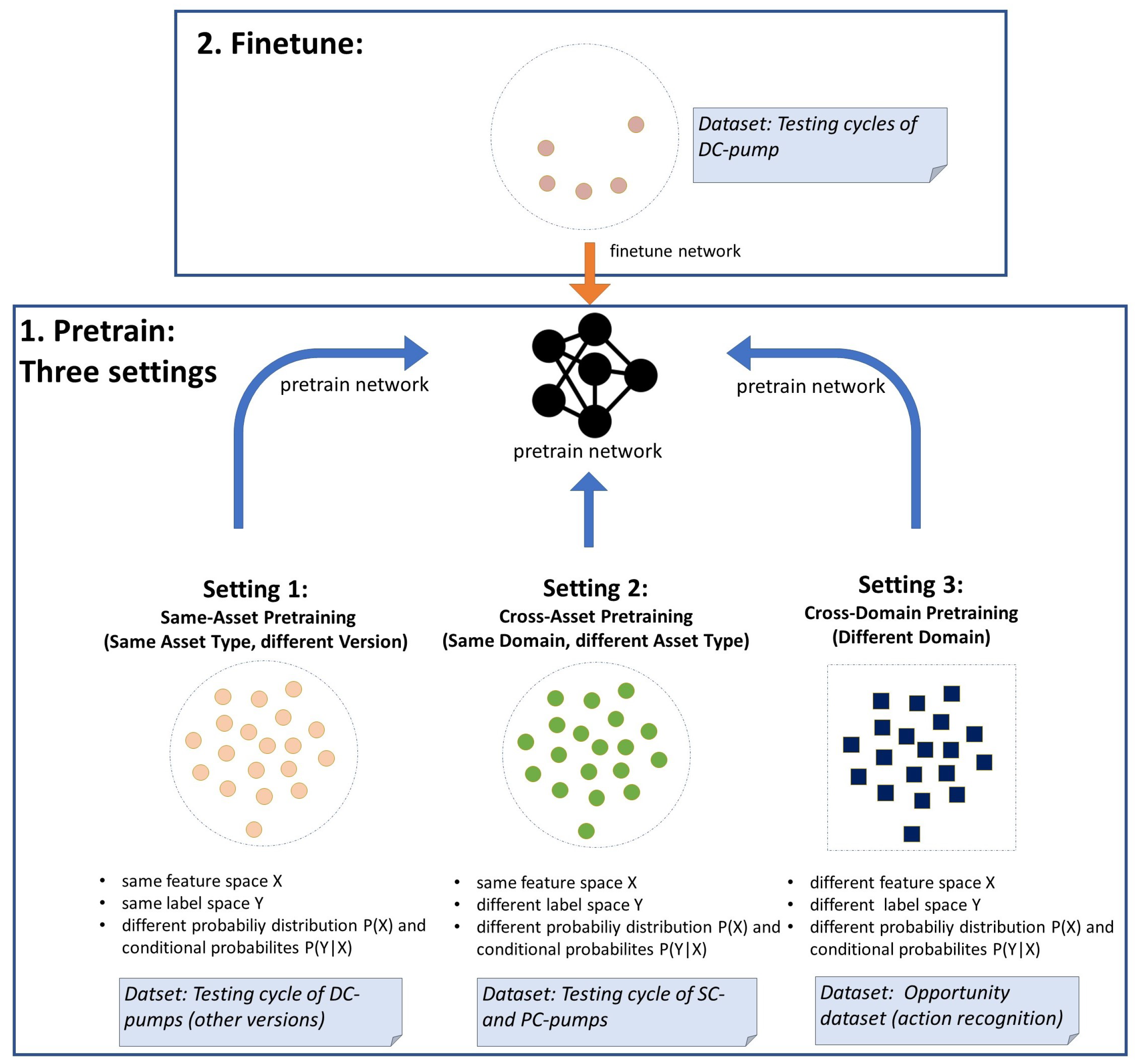
The experimental setup consists of three settings with varying
source datasets (see
Figure 7). The
source datasets were chosen in a way that three varying degrees of similarity between
source dataset and
target dataset are represented in the settings. The
target domains and
target tasks are kept constant over all experiments to enable direct comparability. In each setting, PrecTime is newly pretrained by the
source dataset, before being finetuned by the
target dataset. As the amount of samples used for training might seem very low for deep learning, it has to be noted that in our TSS use case each sample consists of several thousands of labeled datapoints (one label per time stamp). Thus, a far lower number of samples is required to achieve good results compared to other deep learning tasks. The three settings are explained in detail in the following section.
Setting 1 (Same-Asset Pretraining): Source data closely related to target data
In the first setting, both
source datasets and
target datasets are taken from the HPEoL dataset. For the experiment, all three subsets belonging to the DC pump type are selected, with each of the subsets representing the 40 samples of a distinct DC-pump version (V35,V36,V38). The technical design of the three pump versions differs only slightly. In turn, the testing cycles of the three pumps are very similar as well. Only detailed specifications of certain testing phase may vary. Based on the high similarity, we call this setting same-asset pretraining. Using the formalization introduced in
Section 3.1, we have a setting where the feature space X and label space Y of
source data and
target data is identical while the probability distribution P(X) and conditional probabilities
slightly differ. In the experiments, each pump version (V35,V36,V38) is used once as the
target dataset, while the data of the remaining two versions are merged to become the combined
source dataset. For each of these three scenarios, we perform various experimental runs, in which we limit the sample number in the
target training set to 1, 3, 5, and 10. This allows us to investigate how the number of samples in the
target training dataset affects the benefit of pretraining considering training speed and accuracy. Furthermore, two layer freezing approaches are compared. In the first approach all layers except the output layer were frozen (TL-fr). In the second approach all layers were set as trainable (TL-tr). A non-pretrained model that was trained only by the
target dataset is defined as the baseline (BL1). Additionally, as the feature space X and label space Y is identical, an additional baseline can be created by evaluating the model performance when merging the data of all three pump versions to one big training set (BL2). Note that this additional baseline is only available in Setting 1, as it requires equivalence of feature space and label space.
Setting 2 (Cross-Asset Pretraining): Source data distantly related to target data
Like in Setting 1, all source datasets and target datasets are subsets of the HPEoL dataset. However, in this case all three pump types (DC, SC, and PC) are considered. Each of the three DC pump versions (V35,V36,V38) is used as the target data, while both the SC pump subset and the PC pump subset are distinctly used as source data. The testing cycles of the different control types (DC, SC, and PC) differ heavily. However, the used testbenches and sensors are identical across all types. Therefore, we have still have an identical feature space X across source data and target data in this setting. We limit the target domain training data to three instances to make the impact of TL stronger visible. The TL is performed with all layers unfrozen. A non-pretrained model is set as the baseline (BL1).
Setting 3 (Cross-Domain Pretraining): Source data non-related to target data
In Setting 3, it is explored whether pretraining with a non-related
source dataset can boost the accuracy of the
target task. As in Setting 1 and 2, the three DC pump versions are distinctly chosen as
target sets. In this case, however, the pretraining is not done by HPEoL subsets, but by the Opportunity dataset (
Section 3.2). The Opportunity dataset contains sensor location and movement data of human subjects, and, therefore, covers a completely different domain compared to pump testing. Like in setting two, the
target domain training data are limited to three instances and the TL is performed with all layers unfrozen. Again the non-pretrained model BL1 is set as the baseline.
3.5. Implementation Details
The networks were trained on an
NVIDIA Tesla K80 with 6 cores, 56 GB RAM and 380 GB disk storage in the
Microsoft Azure cloud. The implementation was done with
Python mainly utilizing the
Tensorflow and
Keras packages. For the pretraining, all available samples found in the selected
source dataset were used. The
target dataset was split into training set and validation set. The size of the
target training dataset was set to a predefined limited size in each Setting (see
Section 4.3). The training sample size in Setting 1 was varied in different experimental runs (1, 3, 5, 10), while the training sample size in Settings 2 and 3 was kept constant as 3. To achieve comparability, the
target validation set was kept constant across all settings. It was defined to include 20 samples from the
target dataset. The evaluation of the model performance was done by tracking the progress of the validation accuracy for 100 epochs. The accuracy was calculated by dividing the number of time stamps, which were correctly labeled by the mode, by the total number of time stamps. In pretraining, the batch size was defined as 20, while during finetuning it was set equal to the number of training samples. Cross-entropy was chosen as the loss function to be optimized during the training process. The window-size was defined to be 100 in all experiments. The preprocessing included using zero-padding to bring all instances to a fixed length (45000 for HPEoL, 60000 for opportunity). For the Opportunity dataset only the drill-section data were used as samples and 113 sensors were selected as it is common practice in literature [
26]. Missing sensor values were interpolated.
4. Results and Discussion
The following section gives detailed insight into the experimental results and also discusses them.
4.1. Results for Setting 1: Same-Asset Pretraining
Table 1 provides an overview of the achieved validation accuracies in Setting 1. It can be clearly seen that the TL-fr approach (hidden layers set frozen) showed a very weak performance. Thus, the approach seems to be the wrong one for the use case of supervised TSS. In turn, we focus our analysis on TL-tr (all layers unfrozen), which showed a very strong performance in comparison. Pretraining with the
source dataset from the same asset type increased the final accuracy of network in all experiments. A clear negative correlation between the amount of available
target data and the benefit of TL can be observed, meaning TL shows its greatest potential when facing
target data scarcity. While the exact numbers differ in detail, the observations are consistent across all three DC pump versions. When having a
target training set of size one, the accuracy difference between the unfrozen TL-tr approach and the isolated training baseline (BL1) was ranging from 10% for the V38 pump to even 34% for the V35 pump. On the contrary, in the experimental runs using the highest number of
target training samples (10), the performance boost is decreasing to around 2-3%, which is helpful, but far less significant. Interestingly, no clear conclusion could be drawn about the benefit of combining
target data and
source data into one large training set and training the network with it (BL2). While in some experimental runs, the combined training led to accuracy improvement compared to isolated
target data training (BL1), in other cases it seemed to impede model performance. However, note that combining
source data and
training data into one big dataset (BL2) in no case showed a better performance than the TL-tr approach, emphasizing the superiority of using TL in this setting.
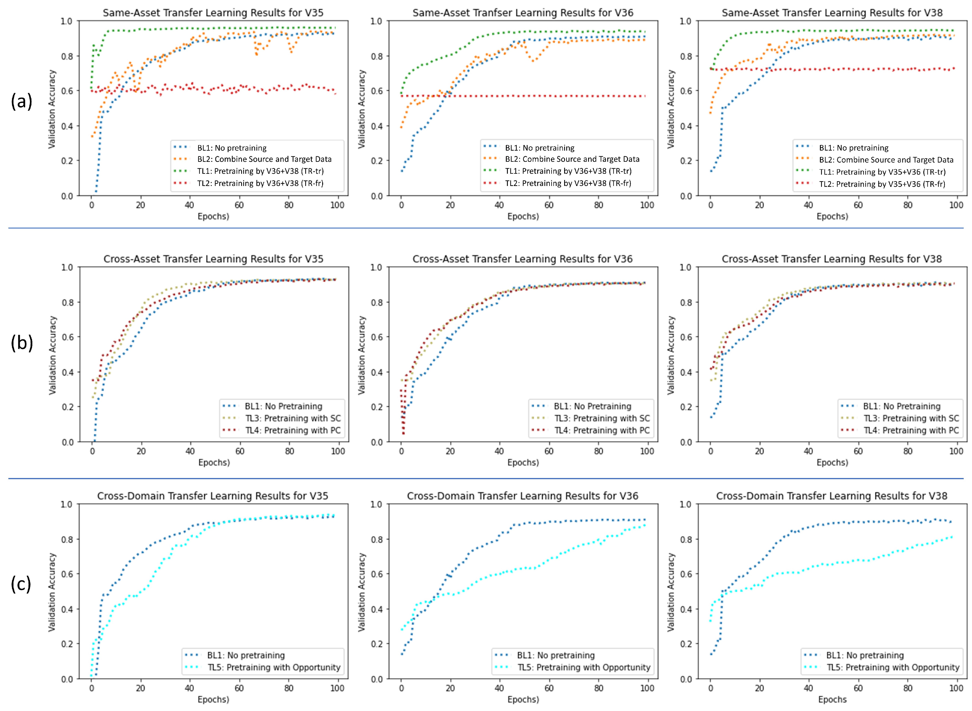
Figure 7.a shows the training progress of all three pump versions for a
target training set of size 3. Clearly, we can observe that for unfrozen TL (TL-tr) not only the final accuracy is improved (higher asymptote), but also the training speed is significantly increased. Very high accuracies (>90%) are reached far earlier compared to the two baselines (BL1, BL2). The main reason of the increased training speed seems to be not a steeper slope, but a higher starting point achieved through pretraining. The extent of this observation varies across the three pumps; it is most visible in the V35 training process. The high starting points after pretraining seem to be the result of using
source data and
training data of high similarity. For frozen TL, it becomes obvious that freezing all hidden layers almost completely eliminates any training progress in this setting. The models end up with almost the same performance before and after finetuning (TL-fr).
4.2. Results for Setting 2: Cross-Asset Pretraining
In Setting 2 (pretraining by
source data from different asset type), the benefits of TL are diminished clearly compared to Setting 1 (see
Table 2). When examining the final model performance, no clear differences (> 1%) across the three pretraining scenarios can be observed for any of the three DC pump versions. Therefore, the potential TL benefit of a higher asymptote is not observed in this setting.
However, when having a closer look on the training progress at
Figure 7.b, we can make an insightful observation. Despite all model training processes ending on a similar performance level after 100 epochs, in the first half of the training process, the models with applied TL show a better performance compared to the models without pretraining. This difference is disappearing more and more in later training stages. This can be explained with the fact that the pretrained models avoid a complete cold start and the pretraining already set parameters in a certain way that helps the
target data training process to progress quicker. Despite the non-identical label space of the
source data and
target data, the pretrained models seem to benefit from a certain relatedness in the nature of the data (shared feature space) at the start of the training.
4.3. Results for Setting 3: Cross-Domain Pretraining
As opposed to the observed benefits of TL in Settings 1 and 2, we can observe a form of negative TL in Setting 3. As the
source dataset (Opportunity) in this setting belongs to a completely different domain than the
target dataset (HPEoL), pretraining does not lead to any benefit, but instead impairs the training speed of the
target data (see
Figure 8c). The different nature of the data prevents a meaningful pretraining that can be exploited later by the
target task. However, despite the slowed training progress, the final asymptote level of the pretrained network (TL5) is similar to or only slightly below that of the non-pretraining scenario (BL1) for all three pump variants. This can be explained with the fact that all layers were set to trainable. Thus, the pretrained models are able to overcome their impaired starting point caused by cross-domain pretraining over the course of the training progress and fully adapt to the new domain.
Altogether, the findings provide systematic evidence for the hypothesis that the benefit of TL in TSS is increasing (1) with lack of
target training data and (2) increasing similarity between
source data and
target data.
Table 3 summarizes the observed results. While we assume these results are to some extent transferable to other domains, further research has to be done to confirm the general validity of our finding.
While freezing layers is often recommended in literature, in this work, it heavily aggravated the model performance in initial experiments (see TL-fr results in Setting 1) and was, therefore, not investigated deeper. However, checking different layer freezing strategies in a more nuanced way might be an interesting direction to go for future research.
5. Conclusion
We performed a systematic investigation of different TL scenarios and strategies for an industrial TSS problem. It was examined whether and how pretraining with close- to non-related source datasets improves the network learning performance of PrecTime, a sequence-to-sequence deep learning architecture for TSS. Focus points were the speed of the training process and the achieved validation accuracy after completing the training. The target task was specified to be the supervised segmentation of hydraulic pump testing cycles into different testing phases via the prediction of state labels. Three different source datasets were selected for pretraining (1) different versions of same pump type, (2) different pump types, and (3) different domains. It was observed that pretraining with a closely-related source dataset led to the biggest benefit (Setting 1), while pretraining with a source dataset from a different domain even aggravated the training progress (Setting 3). Additionally, we could show that TL performed best in comparison to baselines in such scenarios in which the target training dataset had the smallest sample size.
The main limitation of our study is the focus on a specific use case. While our results provide interesting findings, the domain-independence and general validity of the results still have to be established. Furthermore, the important topic of layer freezing was not investigated in depth. Therefore, future work could look deeper into different layer freezing strategies and aim at providing recommendations on which layers should be frozen and which layers set to trainable. Additionally, one could check if incrementally unfreezing layers over the course of the training process leads to promising results. Possible research directions could also include performing experiments with different TSS network architectures and datasets to validate and build on the findings of this paper. It could also be examined how pretraining with multiple datasets or a general-domain dataset affects the model performance. Finally, the transfer of knowledge between labeled data and unlabeled data could investigated in the context of TSS.
Author Contributions
Conceptualization, S.G.; methodology, S.G..; software, S.G.; validation,S.G.; formal analysis, S.G.; investigation, S.G.; resources, S.G.; data curation, S.G.; writing—original draft preparation, S.G.; writing—review and editing, M.R.; visualization, S.G.; supervision, M.R.; project administration, S.G..; funding acquisition, S.G. All authors have read and agreed to the published version of the manuscript.
Funding
This research received no external funding
Institutional Review Board Statement
Not applicable
Informed Consent Statement
Not applicable
Data Availability Statement
Conflicts of Interest
The authors declare that the publication of data must be approved by the Bosch Rexroth AG. The authors declare no conflict of interest. The funders had no role in the design of the study; in the collection, analyses, or interpretation of data; in the writing of the manuscript, or in the decision to publish the results
Sample Availability
Not applicable here.
Abbreviations
The following abbreviations are used in this manuscript:
| ADL |
activities of daily life |
| BL1 |
baseline 1 |
| BL2 |
baseline 2 |
| CNN |
convolutional neural network |
| DC |
direct control |
| HPEoL |
hydraulic pump end-of-line |
| LSTM |
long short-term memory |
| ML |
machine learning |
| PC |
proportional control |
| SC |
speed-based control |
| TL |
transfer learning |
| TSS |
time series segmentation |
References
- Kaveh, A.; Talatahari, S.; Khodadadi, N. Stochastic Paint Optimizer: theory and application in civil engineering. Engineering With Computers, 2022; 1–34. [Google Scholar] [CrossRef]
- Hoppenstedt, B.; Pryss, R.; Stelzer, B.; Meyer-Brötz, F.; Kammerer, K.; Treß, A.; Reichert, M. Techniques and Emerging Trends for State of the Art Equipment Maintenance Systems - A Bibliometric Analysis. Applied Sciences 2018, 8, 1–29. [Google Scholar] [CrossRef]
- Hoppenstedt, B.; Reichert, M.; Kammerer, K.; Probst, T.; Schlee, W.; Spiliopoulou, M.; Pryss, R. Dimensionality Reduction and Subspace Clustering in Mixed Reality for Condition Monitoring of High-Dimensional Production Data. Sensors 2019, 19, 3303. [Google Scholar] [CrossRef] [PubMed]
- Kammerer, K.; Hoppenstedt, B.; Pryss, R.; Stökler, S.; Allgaier, J.; Reichert, M. Anomaly Detections for Manufacturing Systems Based on Sensor Data–Insights into Two Challenging Real-World Production Settings. Sensors 2019, 19. [Google Scholar] [CrossRef] [PubMed]
- Phan, H.; Andreotti, F.; Cooray, N.; Chén, O.; de Vos, M. SeqSleepNet: End-to-End Hierarchical Recurrent Neural Network for Sequence-to-Sequence Automatic Sleep Staging 2018.
- Gaugel, S.; Reichert, M. PrecTime: A Deep Learning Architecture for Precise Time Series Segmentation in Industrial Manufacturing Operations, PrePrint (www.academia.edu), 2023.
- Lu, N.; Hu, H.; Yin, T.; Lei, Y.; Wang, S. Transfer Relation Network for Fault Diagnosis of Rotating Machinery With Small Data. IEEE transactions on cybernetics 2021, PP. [Google Scholar] [CrossRef] [PubMed]
- Cao, P.; Zhang, S.; Tang, J. Preprocessing-Free Gear Fault Diagnosis Using Small Datasets With Deep Convolutional Neural Network-Based Transfer Learning. IEEE Access 2018, 6, 26241–26253. [Google Scholar] [CrossRef]
- Matias, P.; Folgado, D.; Gamboa, H.; Carreiro, A. Time Series Segmentation Using Neural Networks with Cross-Domain Transfer Learning. Electronics 2021, 10, 1805. [Google Scholar] [CrossRef]
- Zhuang, F.; Qi, Z.; Duan, K.; Xi, D.; Zhu, Y.; Zhu, H.; Xiong, H.; He, Q. A Comprehensive Survey on Transfer Learning. Proceedings of the IEEE 2021, 109, 43–76. [Google Scholar] [CrossRef]
- Weber, M.; Auch, M.; Doblander, C.; Mandl, P.; Jacobsen, H.A. Transfer Learning With Time Series Data: A Systematic Mapping Study. IEEE Access 2021, 9, 165409–165432. [Google Scholar] [CrossRef]
- Maschler, B.; Weyrich, M. Deep Transfer Learning for Industrial Automation: A Review and Discussion of New Techniques for Data-Driven Machine Learning. IEEE Industrial Electronics Magazine 2021, 15, 65–75. [Google Scholar] [CrossRef]
- Li, W.; Gao, H.; Su, Y.; Momanyi, B.M. Unsupervised Domain Adaptation for Remote Sensing Semantic Segmentation with Transformer. Remote Sensing 2022, 14. [Google Scholar] [CrossRef]
- Liu, X.; Yoo, C.; Xing, F.; Oh, H.; Fakhri, G.; Kang, J.W.; Woo, J. Deep Unsupervised Domain Adaptation: A Review of Recent Advances and Perspectives. APSIPA Transactions on Signal and Information Processing 2022. [Google Scholar] [CrossRef]
- Heistracher, C.; Jalali, A.; Strobl, I.; Suendermann, A.; Meixner, S.; Holly, S.; Schall, D.; Haslhofer, B.; Kemnitz, J. Transfer Learning Strategies for Anomaly Detection in IoT Vibration Data. IECON 2021 – 47th Annual Conference of the IEEE Industrial Electronics Society. IEEE, 10/13/2021 - 10/16/2021, pp. 1–6. [CrossRef]
- He, Q.Q.; Pang, P.C.I.; Si, Y.W. Multi-source Transfer Learning with Ensemble for Financial Time Series Forecasting; 2021; pp. 227–233. [CrossRef]
- Yan, J.; Wang, L.; He, H.; Liang, D.; Song, W.; Han, W. Large-Area Land-Cover Changes Monitoring With Time-Series Remote Sensing Images Using Transferable Deep Models. IEEE Transactions on Geoscience and Remote Sensing 2022, 60, 1–17. [Google Scholar] [CrossRef]
- Lian, R.; Tan, H.; Peng, J.; Li, Q.; Wu, Y. Cross-Type Transfer for Deep Reinforcement Learning Based Hybrid Electric Vehicle Energy Management. IEEE Transactions on Vehicular Technology 2020, 69, 8367–8380. [Google Scholar] [CrossRef]
- Aldayel, M.S.; Ykhlef, M.; Al-Nafjan, A.N. Electroencephalogram-Based Preference Prediction Using Deep Transfer Learning. IEEE Access 2020, 8, 176818–176829. [Google Scholar] [CrossRef]
- Gross, J.; Buettner, R.; Baumgartl, H. Benchmarking Transfer Learning Strategies in Time-Series Imaging: Recommendations for Analyzing Raw Sensor Data. IEEE Access 2022, 10, 16977–16991. [Google Scholar] [CrossRef]
- Wen, T.; Keyes, R. Time Series Anomaly Detection Using Convolutional Neural Networks and Transfer Learning. [CrossRef]
- Gikunda, P.; Jouandeau, N. Homogeneous Transfer Active Learning for Time Series Classification; pp. 778–784. [CrossRef]
- Warushavithana, M.; Mitra, S.; Arabi, M.; Breidt, J.; Pallickara, S.L.; Pallickara, S. A Transfer Learning Scheme for Time Series Forecasting Using Facebook Prophet; pp. 809–810. [CrossRef]
- Fawaz, H.I.; Forestier, G.; Weber, J.; Idoumghar, L.; Muller, P.A. Transfer learning for time series classification. 2018 IEEE International Conference on Big Data (Big Data), 2018; 1367–1376. [Google Scholar]
- Dridi, A.; Afifi, H.; Moungla, H.; Boucetta, C. Transfer Learning for Classification and Prediction of Time Series for Next Generation Networks; pp. 1–6. [CrossRef]
- Yao, R.; Lin, G.; Shi, Q.; Ranasinghe, D. Efficient Dense Labeling of Human Activity Sequences from Wearables using Fully Convolutional Networks. [CrossRef]
- Maschler, B.; Vietz, H.; Jazdi, N.; Weyrich, M. Continual Learning of Fault Prediction for Turbofan Engines using Deep Learning with Elastic Weight Consolidation; pp. 959–966. [CrossRef]
- Kammerer, K.; Pryss, R.; Reichert, M. Context-Aware Querying and Injection of Process Fragments in Process-Aware Information Systems. 2020 IEEE 24th International Enterprise Distributed Object Computing Conference (EDOC), 2020, pp. 107–114. [CrossRef]
- Maschler, B.; Knodel, T.; Weyrich, M. Towards Deep Industrial Transfer Learning for Anomaly Detection on Time Series Data; pp. 01–08. [CrossRef]
- Tercan, H.; Guajardo, A.; Meisen, T. Industrial Transfer Learning: Boosting Machine Learning in Production. 2019 IEEE 17th International Conference on Industrial Informatics (INDIN). IEEE, 7/22/2019 - 7/25/2019, pp. 274–279. [CrossRef]
- Zhou, X.; Zhai, N.; Li, S.; Shi, H. Time Series Prediction Method of Industrial Process with Limited Data Based on Transfer Learning. IEEE Transactions on Industrial Informatics, 2022; 1–10. [Google Scholar] [CrossRef]
- Xu, W.; Wan, Y.; Zuo, T.Y.; Sha, X.M. Transfer Learning Based Data Feature Transfer for Fault Diagnosis. IEEE Access 2020, 8, 76120–76129. [Google Scholar] [CrossRef]
- Wu, S.; Jing, X.Y.; Zhang, Q.; Wu, F.; Zhao, H.; Dong, Y. Prediction Consistency Guided Convolutional Neural Networks for Cross-Domain Bearing Fault Diagnosis. IEEE Access 2020, 8, 120089–120103. [Google Scholar] [CrossRef]
- Xu, G.; Liu, M.; Jiang, Z.; Shen, W.; Huang, C. Online Fault Diagnosis Method Based on Transfer Convolutional Neural Networks. IEEE Transactions on Instrumentation and Measurement 2020, 69, 509–520. [Google Scholar] [CrossRef]
- He, Y.; Tang, H.; Ren, Y. A Multi-channel Transfer Learning Framework for Fault Diagnosis of Axial Piston Pump. In 2021 Global Reliability and Prognostics and Health Management (PHM-Nanjing); 2021; pp. 1–7. [CrossRef]
- Lin, Y.P.; Jung, T.P. Improving EEG-Based Emotion Classification Using Conditional Transfer Learning. Frontiers in Human Neuroscience 2017, 11. [Google Scholar] [CrossRef] [PubMed]
- Sun, S.; Shi, H.; Wu, Y. A survey of multi-source domain adaptation. Information Fusion 2015, 24, 84–92. [Google Scholar] [CrossRef]
- Chambers, R.D.; Yoder, N.C. FilterNet: A Many-to-Many Deep Learning Architecture for Time Series Classification. Sensors (Basel, Switzerland) 2020, 20. [Google Scholar] [CrossRef] [PubMed]
- Chavarriaga, R.; Sagha, H.; Bayati, H.; Millan, J.d.R.; Roggen, D.; Förster, K.; Calatroni, A.; Tröster, G.; Lukowicz, P.; Bannach, D.; Kurz, M.; Hölzl, G.; Ferscha, A. Robust activity recognition for assistive technologies: Benchmarking machine learning techniques. 2010.
|
Disclaimer/Publisher’s Note: The statements, opinions and data contained in all publications are solely those of the individual author(s) and contributor(s) and not of MDPI and/or the editor(s). MDPI and/or the editor(s) disclaim responsibility for any injury to people or property resulting from any ideas, methods, instructions or products referred to in the content. |
© 2023 by the authors. Licensee MDPI, Basel, Switzerland. This article is an open access article distributed under the terms and conditions of the Creative Commons Attribution (CC BY) license (http://creativecommons.org/licenses/by/4.0/).
