Preprint
Article

A Mixed Clustering Approach for Real Time Anomaly Detection

Altmetrics

Downloads

164

Views

31

Comments

0

A peer-reviewed article of this preprint also exists.

This version is not peer-reviewed

Submitted:

01 March 2023

Posted:

02 March 2023

You are already at the latest version

Alerts
Abstract
Anomaly Detection in real time data is accepted as a vital research area. Clustering has effectively been tried for this purpose. As the datasets are real time, the time of generating of the data is also important. In this article, we introduce a mixture of partitioning and agglomerative hierarchical approach to detect anomalies from such datasets. It is a two-phase method which follows partitioning approach first and then agglomerative hierarchical approach. The dataset can have mixed attributes. In phase-1, a unified metric defined on mixed attributes is used. The same is also used for merging of similar clusters in phase-2. Also, we have kept the track of time attribute of each data instance which produces the clusters with their lifetimes in phase-1. Then in phase-2, we merge the similar clusters. While merging, the similar clusters, the lifetimes of the corresponding clusters with overlapping cores are to be superimposed producing fuzzy time intervals. This way, each cluster will have an associated fuzzy lifetime. The data instances either belonging sparse clusters or not belonging to any of the clusters can be treated as anomalies. The efficacy of the algorithms can be established using both complexity analysis as well as experimental studies.
Keywords: 
Subject: Computer Science and Mathematics  -   Data Structures, Algorithms and Complexity

1. Introduction

The widespread use of computers, databases and associated networks makes them vulnerable to attacks. The attacks are in the form hacking or intruding and which are actually malicious activities to undermine the integrity or security of the systems or their resources. We term them as anomalous activities and data instances associated with the activities as anomalies. An anomaly is the data object [1,2] which deviates, from the previously observed one. Detection of anomalies is now accepted as hot area of modern research.
Intrusion Detection Systems (IDS) are security tools that provide the safety, the security and the strength to any information and communication systems [3]. Recently, anomaly-based IDSs [4] are gaining popularity because of extensive use and their ability to detect insider attack or previously unknown attack. There are several approaches of IDS and one such approach is data mining-based approach.
Data mining is usually an iterative and interactive pattern finding process and its goal is to find patterns, associations, correlations, variations, anomalies, and similar statistically noteworthy structures from large datasets [5]. There are three fundamental practices of data mining namely unsupervised, supervised and semi-supervised learning [6]. Clustering [7] is an unsupervised learning practice frequently exercised to unearth patterns and distribution of data. While it has been widely used in social science and psychology [8], there are several algorithms developed for this purpose namely k-means, k-medoid, CLARA, CLARAN, ROCK, CACTUS, DBSCAN [7,8,9,10,11] etc. In [12], the authors have proposed a hierarchical algorithm which can be used for both static as well as dynamic datasets.
Static clustering mostly deals with the static dataset that are ready before the use of the algorithm. In [13], the authors have proposed several incremental clustering algorithms that can process new record or data instance as they are added to the dataset. However, there are some applications like Wireless Sensor Networks, IOT, Cloud, Finance and Social etc. where data are real time.
Clustering has been widely employed in many areas of anomaly detections. Using Weighted-Euclidean distance function in [14], anomaly detection techniques is proposed for traffic-anomaly detection. In [15], the authors have evaluated performance of k-means clustering-based anomaly detection method using KDD Cup 1999 network dataset. Although a few works have already been completed in this line, most of the aforesaid techniques considered the dataset with numeric attributes. In [16], an algorithm is proposed, which can detect anomalies from the datasets of mixed attributes. Using distance and dissimilarity functions, a fuzzy c-means based clustering method is discussed in [17] which nicely works on both numeric and categorical attributes. In [18], an approach for anomaly detection of mixed attribute-dataset is proposed which follows both partitioning and hierarchical approaches. Although most of the above-mentioned works are on static dataset, the anomaly detection from real time data is found to be interesting and it has caught attention to many researchers. In [19], the authors have proposed an anomaly detection technique of the aforesaid data which can be applicable to both multi-dimensional as well as categorical data. In [20], the authors have introduced time series data cube as new data structure in handling multi-dimensional data for the anomaly detection. Gupta et al [21], have made detailed study on anomaly detection of strictly temporal data for both discrete and continuous cases. In [22], the authors have presented a classification-based method of online detection of anomalies from highly unreliable data. In [23], a sequential k-means algorithm is presented where cluster-center are updated with the arrival of each data instance. In [24], an efficient online anomaly detection algorithm for data streams is proposed which takes into consideration the temporal proximity of the data instances.
In this article, we have put forwarded an anomaly detection algorithm for real time data with mixed attributes using clustering techniques. The algorithm follows both partitioning and agglomerative hierarchical approaches and each cluster produced by the method will have an associated fuzzy time interval as its lifetime. The algorithm starts with partitioning approach then follows agglomerative hierarchical approach. As the data in the dataset are real time like data stream, the time of generation of every data instance is important and the algorithm also takes this into account. The objective of this article is as follows. First of all, we define the data instance-cluster distance measure [10,18] in terms of both numeric and categorical attribute-cluster distance. After this, the similarity of a pair of clusters is expressed in an equivalent manner and a merge function based on the similarity is defined. Finally, a two-phase method for anomaly detection is proposed. In the phase-1, the first k- data instances are kept in k-different clusters along with their time stamps (time of generation) as cluster creation times or start time of the lifetimes. If a new data instance comes to any of the k-clusters, the lifetime of the cluster is extended by the current time stamp. Then the cluster’s categorical attribute’s frequency and the numeric value’s mean are updated. At the end of phase-1, each cluster is having an associated lifetime. Then agglomerative hierarchical approach starts. In this phase, a merge function based on similarity measure is used to merge two highly similar clusters if their lifetimes overlap. Then the overlapping lifetimes are kept in a compact form using set superimposition [25,26]. For the merger of the clusters at any stage two superimposed intervals are superimposed based on non-empty intersection of their cores. This way each resulting cluster will have an associated superimposed time interval [26] which produces a fuzzy time interval. The algorithm stops when no further merger is possible. The algorithm supplies set of clusters where each cluster will have an associated fuzzy time interval as its lifetime. One challenging issue in partitioning clustering is to specify the value of k and there are several methods developed for this purpose. Our algorithm has addressed this problem nicely by producing same number of stable clusters irrespective of the number of input clusters because numbers clusters will be reduced during merging phase. Clearly, the order of the output cluster set will be less than or equal to k. Thus, the output cluster set is more stable and invariant with respect to the number of input clusters. The data instances which either belong to sparse clusters or does not belong to any of the clusters will be considered as anomalies. The method’s efficacy is established using complexity analysis and experimental evaluation.
The article is arranged as follows. The recent developments in this area are explained in Section-2. In Section-3, we discuss the terms, notations and definitions that has been used here. In Section-4, we explain the proposed system using algorithm and flowchart. The complexity analysis is done in Section-5, and the results and findings of the experimental studies are given in Section-6, Finally, we wind-up the paper with conclusions and lines for future works in Section-7.

2. Related Works

Anomaly detection is the finding of the data object which deviates, from the previously observed one. In [1,2] the authors have discussed about anomalies and different clustering-based techniques and algorithm to identify them. Intrusion Detection Systems (IDS) are protection steps that can assure the safety and the security from unauthorized access [3]. There are several well-known IDS available and signature detections system [3] is one them. Off late the anomaly-based IDSs [4] are gaining popularity because of their wide-spread use and ability to detect insider attack or previously unknown attack. Most of the anomaly-based IDS follows clustering or classification approaches.
Data mining is a well-known area of research which includes techniques to discover pattern from large datasets. The most popular data mining tasks includes pattern mining, association rule mining, clustering, classification, anomaly detections etc. [5,6]. Clustering [7] is a popular technique used to find patterns and data distributions in datasets and it has extensively been used in many fields of human knowledge [7,8,9,10,11]. In [12], the authors have proposed a hierarchical algorithm which can be applied for both static as well as dynamic datasets. In [13], the authors have proposed several incremental clustering algorithms that can process new record or data instance as they are added to the dataset.
In [14], the authors have used Weighted-Euclidean distance function in k-means clustering algorithm for traffic-anomaly detection. In [15], the authors have studied the performance of k-means-based anomaly detection method. In [16] a hierarchical agglomerative algorithm is proposed for the anomaly detection in the datasets with mixed attributes. Based on minimization of cluster compactness and maximization of cluster separation in [27], the authors have proposed an anomaly detection technique. In [16], an R-based implementation of DBSCAN is proposed.
In [18], the authors have proposed a hybrid approach consisting of both partitioning and hierarchical algorithm for anomaly detections from the datasets with mixed attributes. In [19], the authors have proposed an anomaly detection technique of aforesaid data which can be applicable to both multi-dimensional as well as categorical data. In [20], the authors have introduced time series data cube as new data structure in handling multi-dimensional data for the anomaly detections. Gupta et al [21], have made detailed study on anomaly detection of strictly temporal data for both discrete and continuous cases. In [22], the authors have presented a classification-based method of on-line detection of anomalies from highly unreliable data. In [29], the authors have put forwarded a hybrid semi-supervised method for finding anomalies in high dimensional data. In [30], the authors have proposed a method using random forests for the improvement of the anomaly detection rate for streaming datasets.
Fuzzy is brought into clustering and anomaly detection by Linquan et al [17]. Using distance and dissimilarity functions a fuzzy c-means based method is discussed in [17] which nicely works both numeric and categorical attributes. In [31], the authors have made a detailed study on intrusion detection systems, fuzzy anomaly detection approach along with their advantages and limitations. In [32], the authors have proposed an algorithm to detect anomalies from temporal data. In [33], the authors proposed a real-time eGFC, to the log-based anomaly detection problem with time-varying data from the Tier-1 Bologna computer center. In [34], the authors have discussed a model using the association between fuzzy logic and ANN to recognize anomalies in transactions involved in the context of computer networks and cyberattacks. A sequential k-means clustering algorithm which updates cluster-center with the new arrival of each data instance is proposed in [23]. An efficient online anomaly detection algorithm based on temporal proximity is proposed in [24].
In [18], the authors introduced a set operation called superimposition which can be used on overlapping intervals to generate superimposed intervals. Applying Glivenko-Cantelli Lemma [35] of order statistics on superimposed intervals, fuzzy intervals can be generated [18]. In [26], the authors have used the set superimposition on locally frequent itemsets to generate periodically frequent itemsets from temporal datasets which in turn gives fuzzy periodic patterns. In [11], the same operation is used and with help of fuzzy variance for the clustering of frequent patterns. In [36], the authors have used set superimposition to solve a simple fuzzy linear equation. In this article we are using the aforesaid operation to find out the fuzzy time interval associated with each cluster as its lifetime.

3. Problem Definitions

In this section, we will navigate some significant terms, definitions, and formulae to be used in the proposed algorithm. Since most of the real-life datasets are hybrids, and the k-Means algorithm uses the distance between the object and the cluster, typical distance formulae do not work. Therefore, it is required to formulate a general distance function which can be appropriate for numeric, categorical, or hybrid attributes. The formulae are given below.
  • Definition 3.1 Distance in Categorical Attributes.
In [10,18], the authors have formulated a distance function for categorical attribute as follows. If the data instances set have categorical attributes A1, A2, ….Ad. The domain (Ai; i=1,2,…d)={ai1, ai2,…aim} comprises-finite, unordered possible values that can be taken by each attribute Ai, such that for any a, b∈dom(Ai), either a=b or a≠b. Any data instance xi is a vector (xi1, xi2,….xid)/, where xipdom(Ap), p=1,2,…d. The distance d(xi, Cj) between data instance xi and cluster Cj, i=1, 2,…n and j=1,2,….k. as proposed in [10,18] is given by
d ( x i , C j ) = p = 1 d w p d ( x i p , C j ) , w h e r e p = 1 d w p = 1
Here wi, the weight factor associated with each attribute, describes the importance of the attribute which controls the contribution attribute-cluster distance to data instance-cluster distance. The attribute-cluster distance between xip and Cj is proposed in [10,18] as follows.
d ( x i p , C j ) = | C j ( A p = x i p ) | | C j ( A p ϕ ) |
Obviously d(xip, Cj) ∈ [0,1] means d(xip, Cj)=1 only if all the data instance in Cj for which Ap=xip and d(xip, Cj)=0 only if no data instance in Cj for which Ap=xip. With the help of equation (2), equation (1) becomes
d ( x i , C j ) = p = 1 d w p d ( x i p , C j ) = p = 1 d w p | C j ( A p = x i p ) | | C j ( A p ϕ ) |
where d(xi, Cj)∈[0, 1], ,i=1, 2,…n and j=1,2,…k.
  • Definition 3.2 Calculating the Weight of an Attribute.
In [10,37], the formula to calculate the weights of attributes is given as follows. The importance IA of an attribute is quantified by the entropy metric as follows.
I A = ρ ( x ( A ) ) log ( ρ ( x ( A ) ) ) d x ( x )
where x(A) is the value of the attribute A, and ρ (x(A)) is the distribution function of data along A dimension. As the values of categorical attribute are discrete and independent, then an attribute’s probability is computed by counting the frequency of the attribute value. Accordingly, any categorical attribute Ap ‘s (p∈{1,2,…,d}) importance can be evaluated by the formula [10,37].
I A p = t = 1 m p ρ ( a p t ) log ρ ( a p t )
And
ρ a p t = D A p = a p t D A p ϕ
where aptdom(Ap), mp is the A p’s total number of possible values, and D is the whole dataset. From equation (5) it is concluded that an attribute’s importance is directly proportional to the number of different values of the categorical attribute. Although, practically, an attribute with immensely diverse values contributes minimum to the cluster. Hence, equation (5) can further be modified as
I A p = 1 m p t = 1 m p ρ ( a p t ) log ρ ( a p t )
Therefore, we can quantify the importance of an attribute using its average entropy over each attribute value. Hence, each attribute’s weight [10,37] is estimated by.
w p = I A p t = 1 d I A t , p = 1 , 2 , ... , d
Suppose all the attributes make equal contributions in the cluster structure of the data, then, their weights will be constant, i.e. wp=1/d, with p=1,2,…,d [see e.g., [10,37]]. Consequently, the instance or object-cluster distance in equation (3) can be modified as [10,37]
d ( x i , C j ) = 1 d p = 1 d | C j ( A p = x i p ) | | C j ( A p ϕ ) |
  • Definition 3.3 Distance in Numeric Attributes.
The distance formula in [10] for numeric attributes of the data instance is defined as follows. Let xi=(xi1, xi2,…xin) be the numeric attribute of a data instance xi, then the distance d(xi, Cj) between xi; i=1,2,..n and cluster Cj; j=1,2,…k is defined as follows.
d ( x i , C j ) = e ( 0.5 | | x i c j | | 2 ) t = 1 k e ( 0.5 | | x i c t | | 2 )
where cj is the centroid of cluster Cj, and d(xi, Cj)[0, 1].
  • Definition 3.4 Distance in Mixed Attributes.
In [10,37] the distance in mixed attributes is proposed as follows. Suppose xi =[xci, xni], the data instance with xci=(xci1, xci2,… xcidc) categorical and xni=(xni1, xni2,… xnidn) numerical attributes where (dc+dn=d). Using equations (1) and (9), the distance d1(xi, Cj) between the data instance xi and cluster Cj is defined [10,37] as follows:
d 1 ( x i , C j ) = p = 1 d c w p | C j ( A p = x c i p ) | | C j ( A p ϕ ) | + w d c + 1 e ( 0.5 | | x n i c n j | | 2 ) t = 1 k e ( 0.5 | | x n i c n t | | 2 )
Here, p = 1 d c + 1 w p = 1 and cnj is the centroid of cluster Cj.
Since all the data instances-clusters distances are compared and the data instance having minimum data instance-clusters value is to be put in the corresponding cluster, the formula d(xi, Cj) [10,37] can be rewritten as follows:
d ( x i , C j ) = ( 1 p = 1 d c w p | C j ( A p = x c i p ) | | C j ( A p ϕ ) | ) + w d c + 1 e ( 0.5 | | x n i c n j | | 2 ) t = 1 k e ( 0.5 | | x n i c n t | | 2 )
It is worth mentioning here that we subtract the distance in categorical attributes from 1 to fit it on to the same scale as the distance in numeric attributes. Obviously, d(xi, Cj)[0, 1]. If xi∈Cj, d(xi, Cj)=0. In equation (11), the numerical attributes are included as a whole in the Euclidean distance, hence, it can be treated as one of the indivisible components, and only one weight can be assigned to it. Thus, we will have dc+1 attribute weights in total, and their summation is equal to 1. Under such settings, we the attribute weights can be taken as
w d c + 1 = 1 d c + 1
In addition,
w p = d c I A p ( d c + 1 ) t = 1 d I A p , p = 1 , 2 , ... , d c
In this manner, the totat weight of the numeric and categorical parts are 1/(dc+1) and dc/(dc+1) respectively. As the actual weight of each categorical attribute is adjausted by its importance as in equation (7), the equation (12) can give us the weights for mixed attributes.
  • Definition 3.5 Similarity of the Cluster Pair.
Let Ciand Cj { i, j = 1, 2, …k and i≠j } be two clusters obtained by partitioning phase, and ci and cj be their centroids, then the similarity measure [18] S(Ci, Cj) between Ciand Cj is expressed as,
S(Ci, Cj)=(Sn(Ci, Cj)+1-Sc(Ci, Cj))/2
where Sn(Ci, Cj) = the similarity in numeric attributes
= w d c + 1 e 0.5 | | c i c j | | 2 t = 1 k e 0.5 | | c i c t | | 2 + t = 1 k e 0.5 | | c t c j | | 2
and Sc(Ci, Cj) = the similarity of Ci and Cj on categorical attributes [18]
= p = 1 d c w p | C m ( A p = x i p ) | + | C n ( A p = x i p ) | | C m ( A p ) | + | C m ( A p ) | ; i = 1 , 2... m
Using equations (14) and (15), equation (13) becomes [see eg [18]]
S ( C i , C j ) = w d c + 1 e 0.5 | | c i c j | | 2 t = 1 k e 0.5 | | c i c t | | 2 + t = 1 k e 0.5 | | c t c j | | 2 + ( 1 p = 1 d c w p | C m ( A p = x i p ) | + | C n ( A p = x i p ) | | C m ( A p ϕ ) | + | C m ( A p ϕ ) | ) 2
In equation (16), we subtract the similarity in categorical attributes from 1 to make the measure onto same scale as that of numeric attributes. Since Sn (Ci, Cj)[[0,1] and Sc(Ci, Cj)[[0,1], it follows that S(Ci, Cj)[[0,1]. For identical cluster pairs, S(Ci, Cj)=0, and S(Ci, Cj)=1, for completely dissimilar pairs
  • Definition 3.6 Fuzzy Set.
A fuzzy set A in a universe of discourse X is characterized by its membership function μA(x) ∈[0, 1], x∈X where μA(x) represents the grade of membership of x in A. [see e.g., 38].
  • Definition 3.7 Convex Normal Fuzzy Set.
A fuzzy set A is termed as normal [38] if at least one x∈X, for which μA(x) =1. For a fuzzy set A, an α-cut Aα[38] is represented by Aα={x∈X; μA(x)≥α}. If all the α-cuts of A are convex sets then A is said to be convex [38].
  • Definition 3.8 Fuzzy Number.
A convex normal fuzzy set A [38] on the real line R with the property that an x0∈R such that μA(x0) =1, and μA(x) is piecewise continuous is called fuzzy number.
  • Definition 3.9 Fuzzy Interval.
Fuzzy intervals [38] are types of fuzzy numbers such that [a, b]⊂R such that μA(x0)=1for all x0 [a, b], and μA(x)is piecewise continuous.
  • Definition 3.10 Support and core of a fuzzy set
The support of a fuzzy set A in X is the crisp set containing every element of X with membership grades greater than zero in A and is notified by S(A) ={x∈X; μA(x) > 0}, whereas the core of A in X is the crisp set containing every element of X with membership grades 1 in A [see e.g. 38]. Obviously core [t1, t2]=[t1, t2], since a closed interval [t1, t2] is an equi-fuzzy interval with membership 1 [see e. g. 25].
  • Definition 3.11 Set Superimposition.
In [25] an operation named superimposition (S) was proposed. We re-write the operation as follows.
A1 (S) A2 = (A1- A2)(1/2) (+) (A1A2)(1) (+)(A2- A1)(1/2)
Where (A1- A2)(1/2)) and (A2- A1)(1/2) are fuzzy sets having fixed membership (1/2), and (+) denotes union of disjoint sets. To elaborate it, let A1=[x1, y1] and A2=[x2, y2] are two real intervals such that A1 A2≠ϕ, we would get a superimposed portion.
In the superimposition process of two intervals the contribution each interval on the superimposed interval is ½ so from equation (17) we get
[x1, y1](S)[x2, y2]= [x(1),x(2)](1/2) (+) [x(2),y(1)](1) (+) (y(1),y(2)](1/2)
where x(1)=min(x1, x2), x(2)=max(x1, x2), y(1)=min(y1, y2), and y(2)=max(y1, y2)
Similarly, if we superimpose three intervals [x1, y1], [x2, y2], and [x3, y3], with i = 1 3 x i , y i ≠ϕ the resulting superimposed interval will look like
[x1, y1](S)[x2, y2](S)[x3,y3]=[x(1),x(2)](1/3)(+)[x(2),x(3)](2/3)(+) [x(3),y(1)](1) (+) [y(1),y(2)](2/3)(+)[y(2),y(3)](1/3)
[see e.g. [23,24]]
where the sequence {x(i); i-1, 2, 3} is found from {xi; i=1, 2, 3} by arranging ascending order of magnitude and {y(i); i-1, 2, 3} is found from {yi; i=1, 2, 3}in the similar fashion.
Let [xi, yi], i=1,2,…,n, be n real intervals such that i = 1 n [ x i , y i ]  ≠ ϕ. Generalizing (19) we get.
[x1, y1](S) [x2, y2](S) ... (S)[xn, yn] =[x(1), x(2)](1/n) (+) [x(2), x(3)](2/n)(+) ... (+) [x(r), x(r+1)](r/n)(+) ... (+) [x(n), y(1)](1)(+)[y(1),y(2)]((n-1)/n)(+)...(+)[y(n-r),y(n-r+1)](r/n)(+)...(+)[y(n-2),y(n-1)](2/n)(+)[y(n-1),y(n)](1/n)
In (4), the sequence {x(i)} is formed of the sequence {xi} in ascending order of magnitude for i=1,2,…n and similarly {y(i)} is formed of the {yi} in ascending order of magnitude [25]. In (20), we observe that the membership functions are the combination of empirical probability distribution function and complementary probability distribution function and they are given by
γ 1 ( x ) = 0 ,                                       x < x ( 1 )     r 1 m ,       x r 1 < x < x ( r ) 1 ,             x > x ( m )                                    
And
γ 2 ( x ) = 1 ,                                       x < y ( 1 )     1 r 1 n ,       y r 1 < x < y ( r ) 0 ,             x > y ( n )                                    
Using Glivenko-Cantelli Lemma of order statistics [35], the equations (21) and (22), will jointly give us the membership function of the fuzzy interval [see e.g. 25].
  • Definition 3.12 Superimposition of superimposed intervals.
Let A=[x(1), x(2)] (1/m) (+) [x(2), x(3)](2/m) (+) ... (+) [x(r), x(r+1)](r/m) (+) ... (+) [x(m), y(1)](1)(+)[y(1),y(2)]((m-1)/m)(+)...(+)[y(m-r),y(m-r+1)](r/m)(+)...(+)[y(m-2),y(m-1)](2/m)(+)[y(m-1),y(m)](1/m) be the superimposition of m intervals and B=[x(1)/, x(2)/] (1/n) (+) [x(2)/, x(3)/](2/n) (+) ... (+) [x(r)/, x(r+1)/](r/n) (+) ... (+) [x(n)/, y(1)/](1)(+)[y(1)/,y(2)/]((n-1)/n)(+)...(+)[y(n-r)/,y(n-r+1)/](r/n)(+)...(+)[y(n-2),y(n-1)/](2/n)(+)[y(n-1)/,y(n)/](1/n) be superimposition of n intervals, then A(S)B is the superimposition of (m+n) intervals and is given by
A(S)B=[x((1)), x((2))](1/(m+n)) (+) [x((2)), x((3))](2/(m+n))(+) ... (+) [x((m)), x((m+1))](m/(m+n))(+) ... (+) [x((m+n)), y((1))](1)(+)[y((1)),y((2))]((m+n-1)/(m+n))(+)...(+)[y(((m+n-r)),y((m+n-r+1))](r/(m+n))(+)...(+)[y((m+n-2)),y((m+n-1))](2/(m+n))(+)[y((m+n-1)),y((m+n))](1/(m+n))
where{x((1)), x((2)), ..x((m)), x((m+1))…x((m+n))} is the sequence formed from x(1), x(2), ..x(m), x(1)/, x(2)/…x(n)/ in ascending order of magnitude and {y((1)), y((2)), ..y((m)), y((m+1))…y((m+n))} is the sequence formed from y(1), y(2), ..y(m), y(1)/, y(2)/…y(n)/ in ascending order of magnitude. From (24), we get the membership function as
γ 1 ( x ) = 0 ,                                       x < x ( 1 )     r 1 m + n ,       x ( r 1 ) < x < x ( r )       1 ,             x > x ( m + n )                                    
And
γ 2 ( x ) = 1 , x < y ( 1 ) 1 r 1 m + n , y ( r 1 ) < x < y ( r ) 0 , x > y ( m + n )
By the equations (24) and (25), using Glivenko-Cantelli lemma of order statistics [35], we get the membership function of the fuzzy interval generated from the identity (23).
  • Definition 3.13 Merge Function.
Let [ti, ti/] and [tj, tj/] are lifetimes of Ci and Cj {i, j=1,2,…n} respectively such that [ti, ti/][tj, tj/]≠ϕ then the merge() function [18] is defined as C=merge(Ci, Cj)= Ci∪ Cj, if and only if S(Ci, Cj)≤σ, a pre-defined threshold where C is the cluster obtained by merging Ci and Cj. It is to be mentioned here that C will be associated with the superimposed interval [ti, ti/] (S)[tj, tj/] as its lifetime. To merge the clusters with superimposed time intervals, we compute the intersection of the cores of the superimposed time intervals. If it is found to be non-empty, then the clusters are merged and the corresponding superimposed time intervals are again superimposed to get a new superimposed time interval.

4. Proposed Algorithm

We have already mentioned that the proposed algorithm is a two-phase algorithm consisting of both partitioning and agglomerative hierarchical approaches. It is a variation of k-means algorithm which also uses a merge function also. First it follows k-means approach to find k-clusters then the merge function is used to merge similar pairs of clusters. Since the data generated are real time, the algorithm also takes into consideration the time attribute associated with data instances. At the end of phase-1, each resulting clusters will have an associated time interval as its lifetime. During 2nd phase, a pair of similar clusters are merged if they have overlapping-lifetimes (non-empty intersection) and the overlapping time intervals are kept as superimposed interval [Definition of superimposed intervals is given in section-3]. The algorithm is narrated as follows. First of all, the algorithm selects first k, d-dimensional data instances as centroid of k-clusters along with their timestamp (time of generation) as start time of the lifetime. If a data instance is included in a cluster based on its distance with the cluster-centroid, then its time of generation is added to the lifetime to get an updated lifetime, in otherward, the lifetime of the cluster is extended with current time-stamp (time of generation) as the end time of the lifetime. During execution process if a data instance moves from one cluster to another then the lifetimes of both former and later clusters are also updated. For example, if the outgoing data instance has time stamp which is either start time or end time of the former cluster then the lifetime of the former cluster is updated by taking next or previous time stamp of the cluster. The frequency of the categorical and the centroid of the numeric values of the cluster are updated. Again, if the time stamp of outgoing data instance falls within the lifetimes of both former and later clusters then there will not be any changed in the lifetimes of both the clusters however the frequencies of the categorical values and the centroid of the numeric values are updated. Similarly, if the time stamp of data instance moving from one to another cluster falls outside the later cluster’s lifetime then the later cluster’s lifetime is also updated along with its frequency and centroid. Using the above principle, the algorithm computes each incoming data instance’s distance with the centroids of each clusters Cj; j=1,2,3….k, and puts it on the cluster with minimum distance value. It is to be mentioned here that the weights of the categorical attributes are taken to be same. Consequently, the frequency of categorical values, the centroid of the numeric values, and the lifetime of the corresponding cluster are updated. For convenient updating, the centroid of the clusters and the categorical attribute values, two auxiliary matrices are maintained for each cluster, one for storing the frequencies and the other for storing the centroid vectors. Then the weights of the categorical attributes are computed. The process of phase-1 continues till no assignment occurs. At the end of phase-1, each of the k-clusters will have an associated lifetime. In phase-2, the merge function [merge function is defined in Section 3] is applied to the output of phase-1 as follows. Each pair of clusters from k-clusters are merged to produce bigger cluster if their similarity value is within a specified threshold and their lifetimes overlaps. Then overlapping lifetimes will be kept in a compact form as a superimposed time interval which in turn produces fuzzy time intervals. At any intermediate stage of merging, it is required to check the intersection of the cores of the lifetimes of the clusters, to be merged. If they intersect then the clusters are merged along with superimposition two superimposed intervals. The superimposition of two superimposed intervals will produce a new superimposed interval with reconstruction of its membership function [The Definition is given is Section-3]. Again, while merging in the first iteration the lifetimes being closed intervals, their intersection will be computed and if they are found to be non-empty, they will be simply superimposed using the formula of interval superimposition [Definition is given in section-3]. While in the subsequent iterations merging will be associated with the superimposition of the superimposed intervals produced by the previous iteration based on the non-empty intersection of their cores. For storing the boundaries of the time intervals to be superimposed we have used two sorted arrays, one for storing left boundaries and other for right boundaries. The process would continue till no merging of the clusters is possible or a particular level becomes empty. The algorithm produces less than or equal to clusters where each cluster associated with fuzzy time interval as its lifetime. The algorithm is better described with pseudo-code given below
Algorithm1
Step 1: Given an online d-dimensional dataset with both categorical and numeric attributes.
Step 2: Select the number k, to decide the number of clusters.
Step 3: Take first k, data instances and assign them as K-cluster centroid along with their time-stamp as start time of lifetime of the clusters.
Step 4: Assign each incoming data instance to the closest centroid using equal weights for the categorical attributes.
Step 5: Update the two auxiliary matrices maintained for storing the frequency of each categorical value occurring in the cluster, and the mean vector of the numerical parts of all the data instances belonging to the cluster.
Step 6: Extend or update the lifetime of the clusters using the time-stamp of the current data instance to be inserted to the cluster
Step 7: Compute the weights of categorical attributes.
Step 8: if (assignment does not occur)
                    go to step 9.
                    else
                    re-assign each data instance to the new closest centroid of each cluster.
                    go to step 5
Step 9: for each possible pair of clusters (Ci, Cj) with lifetimes as a superimposed intervals S[ti] and S[tj] respectively
                    { if (core(S[ti])∩core(S[tj]) = empty)    break;
           else if (sim(Ci, Cj)<=sigma)
                                        {merge (Ci, Cj);
                                          superimpose the lifetimes
                    }
 continue
}
Step 10: Output clusters

5. Time Complexity

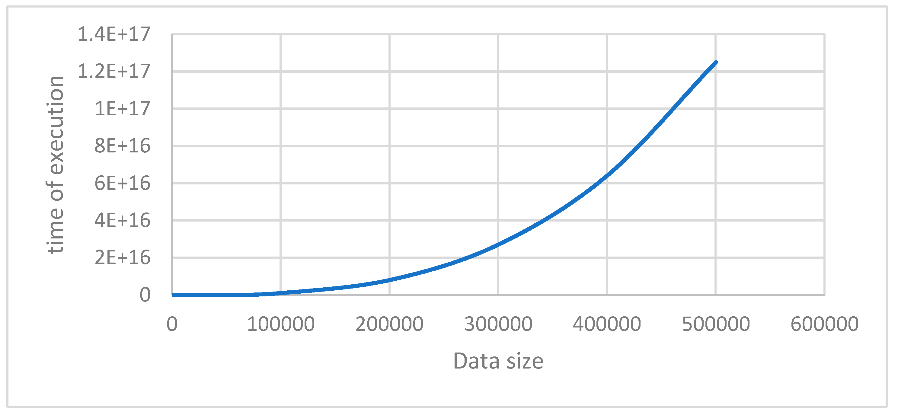
To calculate the time complexity, we proceed as follows. Since the data are real time, it is quite difficult to prefix the number of data instances. Without loss of generality, we assume that the data are finite let say n. Let k (<=n) be the number of clusters and dn= no of numeric attributes and dc= no of categorical attributes so that d=dn+dc+1 = the total number of attributes, where the extra attribute is the time attribute. The computational cost for calculating centroid is O(n+nkdn). The computational cost for step1, step2, and step 3 is O(nkdn). The step 4 take O(kn+nk) time, as for each centroid, the distance of the data instance has to be computed, and minimum distance has to be chosen to assign the data instance in that cluster. The O(nk) time is needed to compute the minimum distance for each k-clusters. Since each data instance is associated with a time stamp it needs another O(nk) time. The cost of updating the two matrices along with lifetimes of clusters is O(3k). This is the computational cost of step 5. Also, the computational cost of updating the weights of categorical attributes is O(ankdc), where a= average number of possible values that the categorical attributes can take. Thus the total computational cost of step 4 and step 5 is O(3k+2nk+ankdc)=O(ankdc). If i be the number of iterations, then the total computational cost for phase-1 is O(i(nkdn+ ankdc))=O(iankdc). For phase-2, we need to merge the clusters obtained during phase-1 based on the non-empty intersection of lifetimes or core(lifetimes) and also a similarity measure. For merging two clusters with lifetimes requires O(n1n2); where n1 and n2 are sizes of the two clusters to be merged. Also, merging is associated with the superimposition of the cluster’s lifetimes. Let m1 are number of intervals superimposed in the lifetime of one cluster and m2 are number of intervals superimposed in the lifetime of another cluster and their cores have non-empty intersection. For the intersection of cores O(1) time is required. If m1 intervals are superimposed in the m2 such that m1<=n and m2<=n, then the boundaries of one superimposed interval are to be inserted on other as two sorted arrays. So, this is basically merging four sorted arrays to produce two sorted arrays one for left end points and others for right end points. The searching in four sorted array requires O(logm1+logm2+ logm1+logm2)=O(4logn)=O(logn) time as m1=O(n) and m2=O(n). The insertion in sorted arrays will require O(m1+m2+m1+m2)=O(4n)=O(n). If t be number of iterations in phase-2, the total cost will be O(t(logn+n))=O(klogn+kn), as t<=k. The total cost of all the steps is O(iankdc+klogn+kn). Since k is constant dc<=n, i<=k<=n, a<=n so i is also constant. The overall complexity of the algorithm is O(n.n.n)=O(n3). Which shows efficacy of the algorithm.

6. Experimental Settings and Discussions

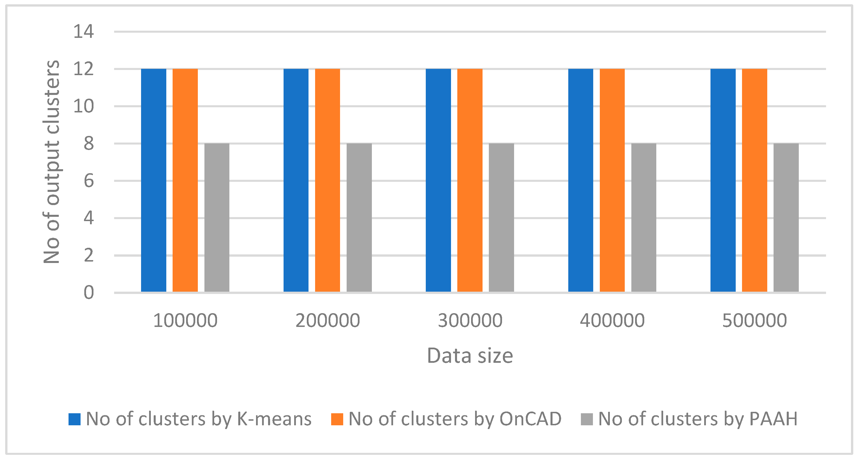
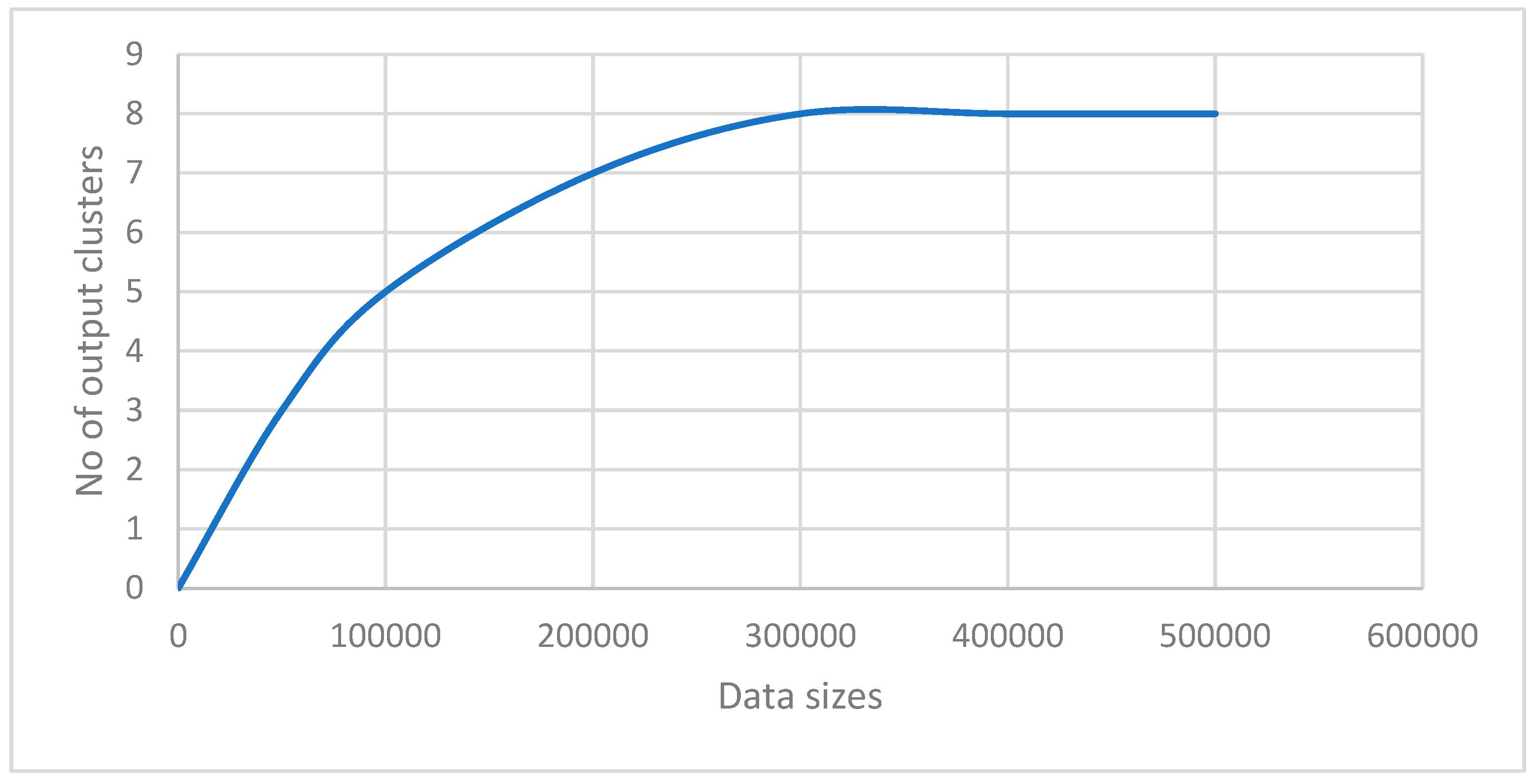
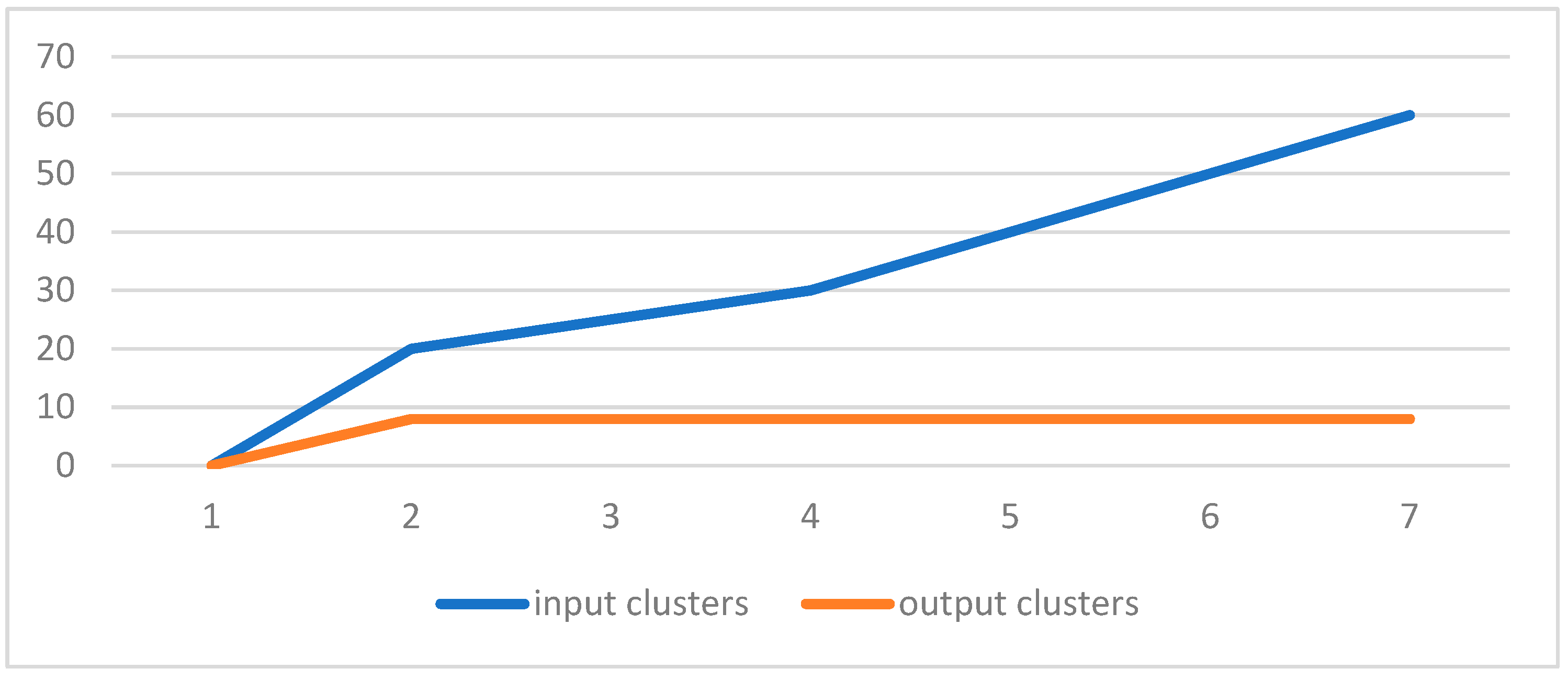
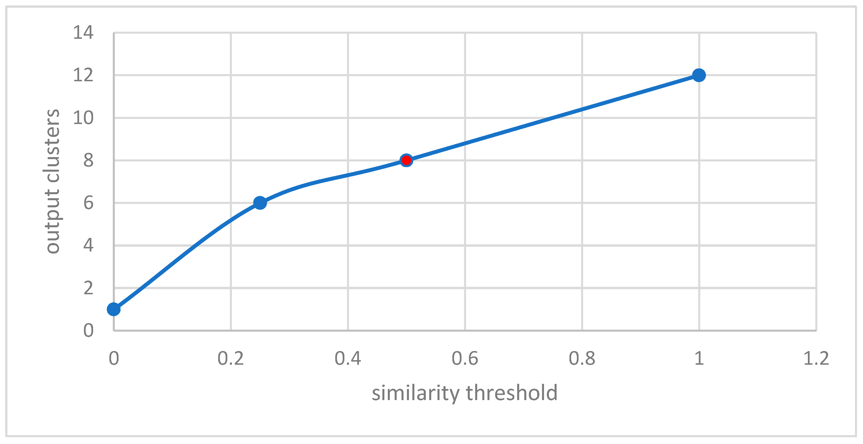
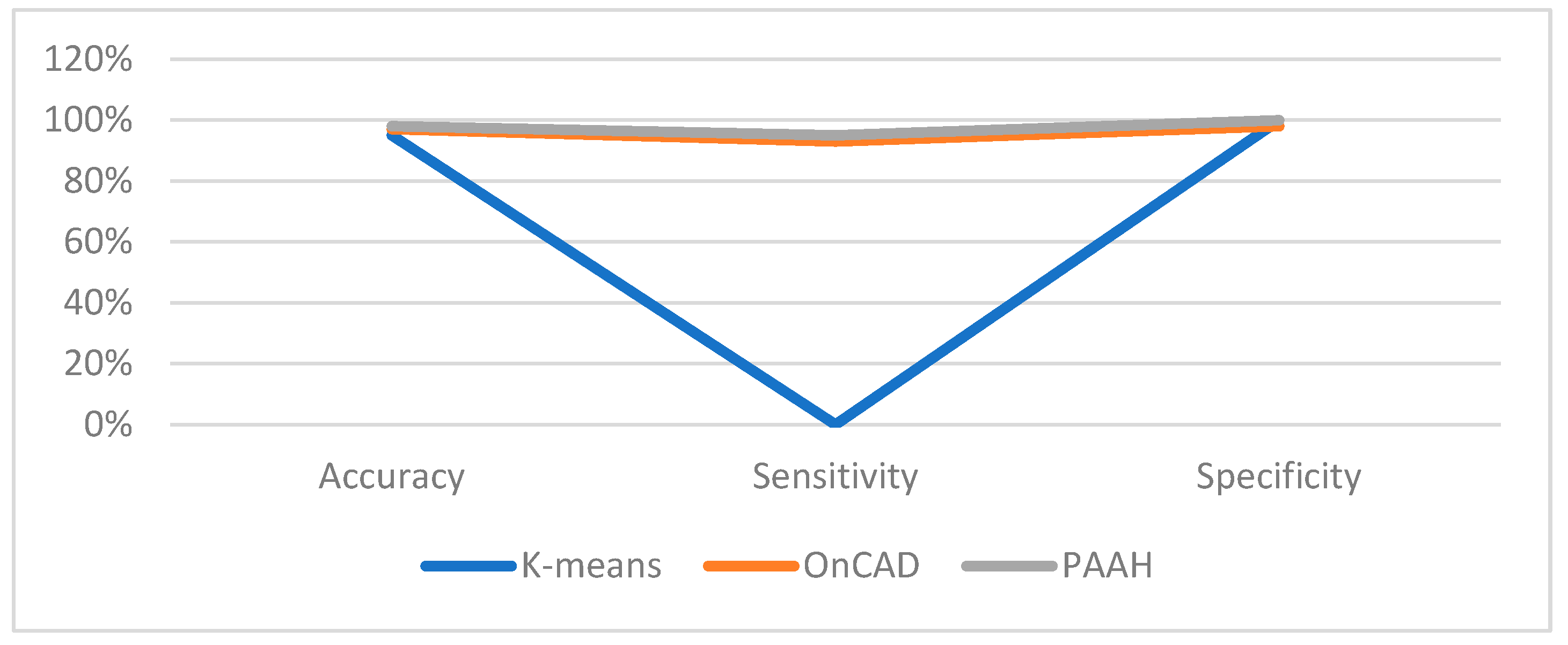
We have made an experimental study with help of a synthetic dataset. We have generated stream of datasets of different sizes with fixed dimension. The generated dataset is quite similar to KDD Cup 99 which has 41 properties with 38 numeric and 3 flag properties. We have taken the dimension of our dataset as 41, with 37 numeric, 3 categorical and 1 temporal attributes (time-stamp). We have also kept the noises from 0 to 5%. The weight of each attribute is assumed to be same. For comparative studies, we have used two algorithms [23,24]. We have implemented the algorithms in MatLab. It has been observed that the aforesaid algorithms work nicely on lower dimensional datasets. Also, they can’t handle categorical attribute values. Also, there is no explicit references of temporal attributes. Secondly, k-means [23] algorithm gives a specified number of clusters which is not realistic in case of real time clustering. OnCAD [24], needs a couple of input parameters to be specified. Our algorithm outperforms the aforesaid algorithms in the sense that it can handle higher dimensional data with numeric, categorical and temporal attributes. The comparative analysis is presented in both tabular form and graphically in Table-1, Table-2, Figure-1 and Figure-2. Although the number of clusters k has to be specified in the partitioning phase, during phase-2, the merge function minimizes the number of clusters. So, even if we start with a large number input clusters, we arrive at quite less number of stable clusters. The similarity threshold has to be adjusted accordingly. In this work, we have taken different values of similarity threshold like 0, 0.25, 0.5, 0.75 to justify our claim. The results are expressed graphically in Figure-3, Figure-4, Figure-5, and Figure-6.
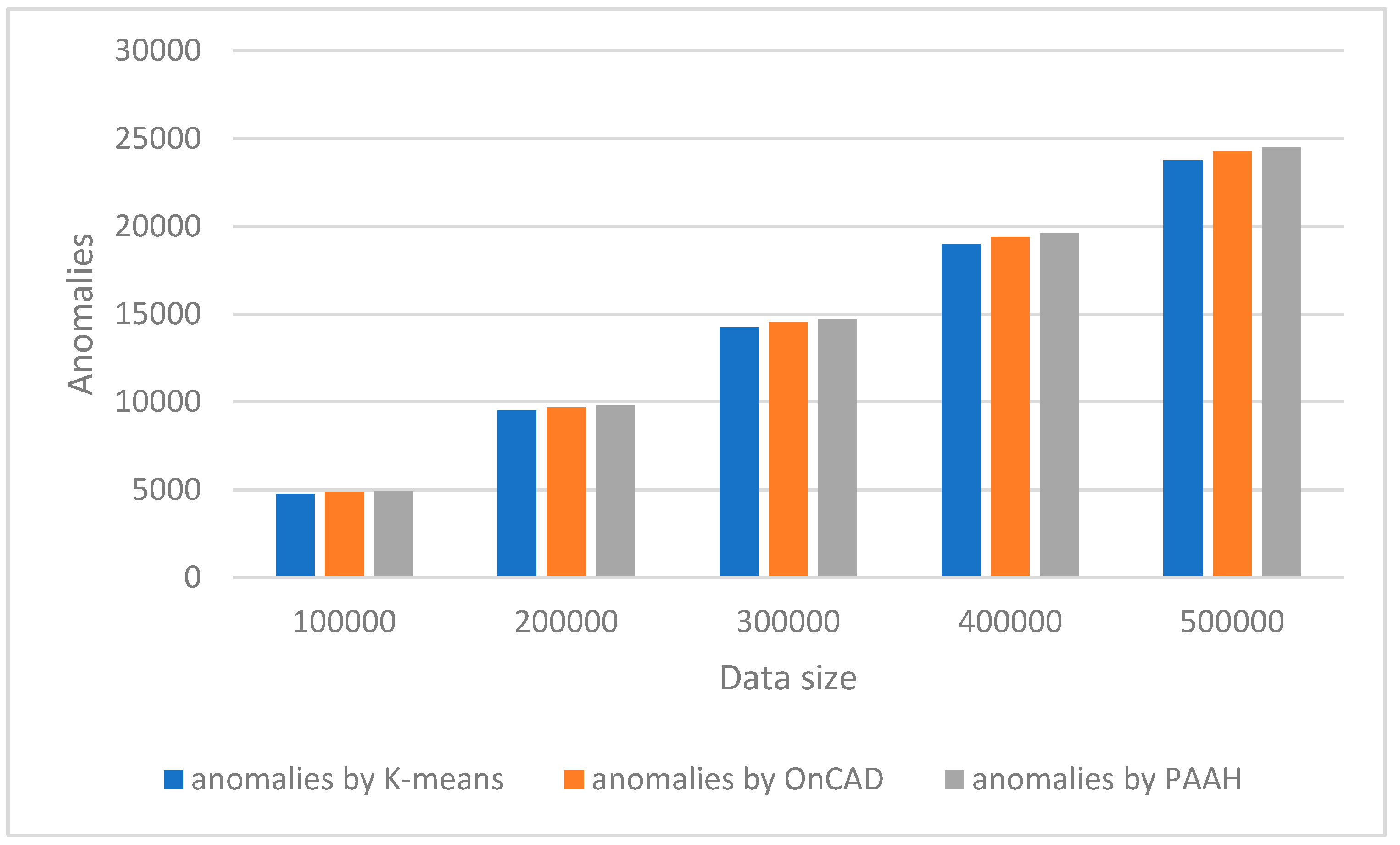
Furthermore, our algorithm explicitly keeps track of the temporal attribute, the time of arrival of data instances as time stamp which others do not. In the first phase, the algorithm generates clusters along with time interval list where each cluster will be associated with a time-interval which later merge to produce clusters with fuzzy time intervals. We have also done the complexity analysis which shows that the algorithm is quite efficient. Also, we have found that our method can extract the anomalies more accurately. The method is scalable in case of data sizes. The results are presented in a tabulated form and graphical in Table-2 and Figure-7.
Table 1. Comparative analysis in terms of different parameters.
Preprints 69315 i002
Figure 1. Comparative analysis.
Preprints 69315 g001
Table 2. Comparative analysis of output clusters.
Preprints 69315 i003
Figure 2. Comparative analysis of output clusters.
Preprints 69315 g002
Table 2. Comparative analysis of anomalies.
Preprints 69315 i004
Figure 3. Comparative analysis of anomalies.
Preprints 69315 g003
Figure 4. Data size vs output cluster.
Preprints 69315 g004
Figure 5. input clusters vs output clusters.
Preprints 69315 g005
Figure 6. Similarity threshold vs output clusters.
Preprints 69315 g006
Figure 7. Data size vs. time of execution.
Preprints 69315 g007

7. Conclusions

In this article, we propose a clustering algorithm for the detection of anomalies for real time data with both numeric and categorical attributes. The algorithm follows both partitioning and agglomerative hierarchical approaches. Each cluster produced by the method will have an associated fuzzy time interval. In the first phase, it follows partitioning approach like k-means clustering algorithm and then it follows agglomerative hierarchical approach. As the dataset is real time consisting data stream, the time of generation of every data instance is important and the algorithm takes this into consideration during execution. In the first phase, initially first k-data instances are kept in k-different clusters along with their time stamp (time of generation) as time of cluster creation or start time of lifetimes of the clusters. If a new data instance enters any of the k-clusters its time stamp is also added to the lifetime. Then frequency of categorical values and mean of numeric values of the cluster will be updated. At the end phase-1, the algorithm supplies a set of k-clusters where each cluster will be having a lifetime. Then agglomerative hierarchical approach starts. In this phase, the algorithm checks whether the lifetime of clusters intersects or not. If intersects then the corresponding clusters are merged based on the similarity value and the resulting lifetimes are kept in a compact form using a method called superimposition [25,26]. This way each resulting cluster will be associated with a superimposed time interval which in turn generates fuzzy time interval [26]. The algorithm stops when no further merger is possible. The algorithm supplies set of clusters where each cluster will have an associated fuzzy time interval as its lifetime. One of the most challenging problems in k-means clustering algorithm is to select the number of input clusters. However, our algorithm has overcome this problem by producing same number of stable clusters irrespective of the number of input clusters. Obviously, the number of output clusters is less than or equal to that at the beginning. The data instance or group of data instances which does not belong to any of the cluster or belongs to sparse clusters will be considered as anomalies. We have made experimental studies with a synthetic dataset and we have shown that our algorithm outperforms two well-known algorithms namely k-means [23] and OnCAD [24] in terms of accuracy, specificity, sensitivity, number of anomalies found, number of clusters generated, execution time and the stability of the output clusters. Furthermore, the output cluster set would be minimal in comparison others. The algorithm is found to be run in cubic time.

Availability Data and Material

The corresponding author states that the data, code and other materials can be made available on request.

DECLARATION

Conflict of Interest/Competing Interest: The corresponding author states that there is no conflict of interest or competing interest exists among the authors.

Ethical statement

The corresponding author states that there is no need of ethical statement as there is no investigation containing animal experimentations, human participations, clinical trials, identifiable human subjects etc.

References

  1. Pamula, R., Deka, J. K. Nandi, S.; “An Outlier Detection Method based on Clustering”, Proceedings of 2011 Second International Conference on Emerging Applications of Information Technology, India (February 2011) 253-256.
  2. Zhang, Y., Liu, J. and Li, H; “An Outlier Detection Algorithm Based on Clustering Analysis”, The Proceedings of 2010 First International Conference on Pervasive Computing, Signal Processing and Applications, September 2010.
  3. Agrawal, S., and Agrawal, J.; “Survey on Anomaly Detection on Data Mining Techniques”, Procedia Computer Science, 60(2015), pp. 708-713.
  4. Pocha, A. and Park, J. M.; “An overview of anomaly detection techniques: Existing solutions and latest technologies”, Computer Networks, 51(12), 2007, pp. 3448-3470.
  5. Zaki, M. J., and Wong, L.; “Data Mining Techniques”, WSPC-2003, Lecture Notes Series. http://www.cs.rpi.edu/~zaki/PaperDir/PGKD04.pdf.
  6. Soni, D.; “Understanding the different types of machine learning”, Towards Data Science, 2019. https://towardsdatascience.com/understanding-the-different-types-of-machine-learning-models-9c47350bb68a.
  7. Hartigan, J. A.; “Hartigan, "Clustering Algorithms", John Wiley & Sons, 1975.
  8. Bailey, K.; "Numerical Taxonomy and Cluster Analysis". Typologies and Taxonomies, (1994). 34.
  9. Gibson, D., Kleinberg, J. and Raghavan, P.; "Clustering categorical data: An approach based on dynamical systems", In Proc. of the 24th Int’l Conf. on Very Large Databases, New York (1998) 311-323. [CrossRef]
  10. Cheng, Yiu-ming, and Jia, H; “A Unified Metric for Categorical and Numeric Attributes in Data Clustering”, Hong Kong University Technical Report (July 2011), http://www.comp.hkbu.edu.hk/tech-report.
  11. Mazarbhuiya, F. A., Abulaish, M.; “Clustering Periodic Patterns using Fuzzy Statistical Parameters”, International Journal of Innovative Computing Information and Control (IJICIC), Vol. 8, No. 3(b), 2012, pp. 2113-2124.
  12. Gil-Garcia, R., Badia-Contelles, J. M, and Pons-Porrata, A.; ” Dynamic Hierarchical Compact Clustering Algorithm”, CIARP 2005, LNCS 3775, pp. 302-310.
  13. Hammouda, K. M., and Kamel, M. S.; “Efficient phrase-based document indexing for web document clustering”. IEEE Transactions on Knowledge and Data Engineering, 16(10):1279–1296, 2004. [CrossRef]
  14. Munz, G., Li, S., and Carle, G.; “Traffic Anomaly Detection using K-Means Clustering”, Allen Institute for Artificial Intelligence, 2007.
  15. Riad, A. M., Elhenawy, Ibrahim, Hassan, Ahmed and Awadallah, N; “visualize network anomaly detection by using k-means clustering algorithm”, International Journal of Computer Networks & Communications (IJCNC) Vol.5, No.5, September 2013.
  16. Mazarbhuiya, F. A. AlZahrani, M. Y. and Georgieva L.; “Anomaly Detection Using Agglomerative Hierarchical Clustering Algorithm”, ICISA 2018, Lecture Notes on Electrical Engineering (LNEE) Volume 514, Springer, Hong Kong, pp 475-484.
  17. Linquan, X., Wang, W., Liping, C., and Guangxue, Y. “An Anomaly Detection Method Based on Fuzzy C-means Clustering Algorithm”, Proceedings of the Second International Symposium on Networking and Network Security, April 2010, China, pp. 089-092.
  18. Mazarbhuiya, F. A. AlZahrani, M. Y. and Mahanta, A. K.; “Detecting Anomaly Using Partitioning Clustering with Merging”; ICIC Express Letters Vol. 14(10), Japan, October 2020, pp. 951-960.
  19. Retting, L., Khayati, M., Cudre-Mauroux, P. and Piorkowski,” 2015 IEEE International Conference on Big Data”, CA, USA.
  20. Li, X. and Han, J.; “Mining approximate top-k subspace anomalies in multi-dimensional time-series data,” in Proceedings of the 33rd International Conference on Very Large Data Bases, Vienna, Austria, September 23-27, 2007, 2007, pp. 447–458.
  21. Gupta, M., Gao, J., Aggrawal, C. C., and Jain, J; “Outlier detection for temporal data: A survey,” IEEE Transactions on Knowledge and Data Engineering, vol. 25, no. 1, pp. 1–1, 2014.
  22. Zhao, Z., Birke, R., Han, R., Robu, B., Bouchenak, S., Ben Mokhtar S., and Chen, L. Y.;” RAD: On-line Anomaly Detection for Highly Unreliable Data”, November 2019. https://arxiv.org/abs/1911.04383.
  23. MacQueen, J.; “Some methods for classification and analysis of multivariate observations,” in Berkeley Symposium on Mathematical Statistics and Probability, vol. 1, no. 14. Oakland, CA, USA., 1967, pp. 281–297.
  24. Chenaghlou, M., Moshtaghi, M., Lekhie, C., and Salahi, M.; “Online Clustering for Evolving Data Streams with Online Anomaly Detection”, Advances in Knowledge Discovery and Data Mining, June 2018, pp. 508-521.
  25. Baruah, H. K.; “The Randomness-Fuzziness consistency principle”, International Journal of Energy, Information and Communications, Vol 1(1), Nov-2010, Japan.
  26. Mahanta, A. K., Mazarbhuiya, F. A., and Baruah, H. K.; “Finding Calendar-based Periodic Patterns”, Pattern Recognition Letters, Vol. 29(9), Elsevier publication, USA, 2008, pp. 1274-1284. [CrossRef]
  27. Alguliyev, R., Aliguliyev, R., and Sukhostat, L., “Anomaly Detection in Big Data based on Clustering” In Statistics, Optimization & Information Computing, Vol. 5, Dec 2017, pp. 325-340.
  28. Zhao, Z., Mehrotra, K. G., and Mohan, C. K.; “Online Anomaly Detection Using Random Forest”, In: Mouhoub M., Sadaoui S., Ait Mohamed O., Ali M. (eds) Recent Trends and Future Technology in Applied Intelligence. IEA/AIE 2018. Lecture Notes in Computer Science, Springer, Cham.
  29. Song, H., Jiang, Z., Men, A., and Yang, B.; “A Hybrid Semi-Supervised Anomaly Detection Model for High Dimensional data”. Computational Intelligence and Neuroscience, Vol 2017, pp. 1-9. [CrossRef]
  30. Zhao, Z., Mehrotra, K. G., and Mohan, C. K.; “Online Anomaly Detection Using Random Forest”, In: Mouhoub M., Sadaoui S., Ait Mohamed O., Ali M. (eds) Recent Trends and Future Technology in Applied Intelligence. IEA/AIE 2018. Lecture Notes in Computer Science, Springer, Cham.
  31. Masdari, M., and Khezri, H.; “Towards fuzzy anomaly detection-based security: a comprehensive review”, Fuzzy Optimization and Decision Making, Vol 20(2001), 2020, pp. 1-49. [CrossRef]
  32. Izakian, H., and Pedrycz, W.; “Anomaly detection in time series data using fuzzy c-means clustering”, In proc. of 2013 Joint IFSA World congress and NAFIPS Annual meeting, Canada.
  33. Decker, L. Leite, D., Giommi, L., and Bonakorsi, D.; “Real-time anomaly detection in data centers for log-based predictive maintenance using fuzzy-rule based approach, April 2020, https://arxiv.org/pdf/2004.13527.pdf.
  34. de Campos Souza, P. V., Guimarães, A. J., Rezende, T. S., Silva Araujo, V. J., and Araujo, V. S.; “Detection of Anomalies in Large-Scale Cyberattacks Using Fuzzy Neural Networks”, AI 2020, 92-116, https://www.mdpi.com/2673-2688/1/1/5. [CrossRef]
  35. Loeve, M. ; “Probability Theory,” Springer Verlag, New York, 1977.
  36. Mazarbhuiya, F. A., Mahanta, A. K., and Baruah, H. K. Baruah,; “The Solution of fuzzy equation A+X=B using the method of superimposition”, Applied Mathematics, 2011, 2, 1039-1045.
  37. Basak, J., and Krishnapuram, R.; “Interpretable hierarchical clustering by constructing and unsupervised decision tree”, IEEE Trans. Knowledge and Data Engineering, vol.17, no.1, pp.121-132, 2005. [CrossRef]
  38. Klir, J., and Yuan, B.; “Fuzzy Sets and Logic Theory and Application”, Prentice Hill Pvt. Ltd. (2002).

Author’s Profile

Preprints 69315 i001 FOKRUL ALOM MAZARBHUIYA received B.Sc. from Assam University, India and M.Sc. from Aligarh Muslim University, India. After that he obtained his Ph.D. in Computer Science from Gauhati University, India. He worked as an Assistant Professor in College of Computer Science and Information Systems, King Khalid University, Saudi Arabia during 2008 to 2011 and, as an Assistant Professor, Information Technology, College of Computer Science and IT, AlBaha University, Saudi Arabia during 2011 to 2018. Since 2019, he is serving as a faculty member in the School of Fundamental & Applied Sciences, Assam Don Bosco University, India. He has published more than 60 research articles in various International and National Journals. His research interest includes Data Mining, Information Security, Fuzzy Mathematics and Fuzzy logic.
MOHAMED SHENIFY received his B.Sc. in computer science from Indiana State University, Terre Haute, Indiana, USA in May 1990; his M.Sc. in computer science from Ball State University, Muncie, Indiana, USA in December 1991 and his PhD in computer science from Illinois Institute of Technology, Chicago, Illinois, USA in May 1998. He is currently working as an Associate Professor at the College of Computer Science and Information Technology (CSIT), Albaha University, Saudi Arabia. His research interests include natural language processing, information retrieval, health care systems, fuzzy logic, and computing education
Disclaimer/Publisher’s Note: The statements, opinions and data contained in all publications are solely those of the individual author(s) and contributor(s) and not of MDPI and/or the editor(s). MDPI and/or the editor(s) disclaim responsibility for any injury to people or property resulting from any ideas, methods, instructions or products referred to in the content.
Copyright: This open access article is published under a Creative Commons CC BY 4.0 license, which permit the free download, distribution, and reuse, provided that the author and preprint are cited in any reuse.
Prerpints.org logo

Preprints.org is a free preprint server supported by MDPI in Basel, Switzerland.

Subscribe

© 2024 MDPI (Basel, Switzerland) unless otherwise stated