Application of Active Disturbance Rejection in a Bearingless Machine with Split Winding

1. Introduction

Magnetically suspended induction machines meet a specific industry demand for less noisy motors that can reach higher speeds and do not cause product contamination in situations where the machine directly handles the process. The induction motor is a multivariable, nonlinear system [1] that has a strong coupling between variables. When used in bearingless systems, the degree of control complexity is even greater, especially when placed in situations with shaft load application. In these cases, linear controllers may not achieve a sufficiently fast and stable response for adequate suspension and control of the other system parameters. The emergence of microprocessor devices and power electronics has provided conditions for the application of advanced control theories such as predictive controllers, sliding mode controllers, neural and artificial network-based controllers, Fuzzy controllers, and others [2]. In recent years, the ADRC Control technique has been used for the control of various types of systems. ADRC Control is a controller originally based on nonlinear functions, composed of three main blocks: Tracking Differentiator (TD), Extended State Observer (ESO), and a block corresponding to the control law that has received different contributions over the years. This work investigated the application of ADRC controllers to the position control of a split-winding induction machine, aiming to understand the limitations of applying this type of controller to the motor-bearing system and to explore the benefits that a technique with active disturbance rejection can bring to radial position control. In [3], [4] investigates the application of the Active Disturbance Rejection Control (ADRC) technique on the stabilization and control of the rotor radial position of a bearingless induction machine with split winding.

2. Split Winding Bearingless Motor

The first split-winding bearing motor was proposed by Salazar & Stephan [5]. They built a 4-pole two-phase motor that used the motor’s torque coils for radial force generation. In this topology, only one of the phases was responsible for radial position control and both phases were used for torque generation. The two-phase motor proposed by [5] was the starting point for the work of [6], who proposed a three-phase motor in which the coils of each phase were divided into two. In this topology, the three phases were used in the generation of radial force and torque. In [7] Paiva’s work, the speed vector control of the three-phase motor-mancal was done using neural networks for rotor flux estimation. In this work, the performance of the machine operating with a conventional state estimator and with a neural state estimator was compared. Valci in [8] analyzed the feasibility of using a conventional induction machine as a split-winding bearingless motor. He performed position and current control of the machine, however, he observed that radial position control was not satisfactory for speeds below rated. In [9] studied the replacement of PID controllers for radial position control with controllers based on Fuzzy logic. Noting the strong nonlinear and parameter-varying characteristics of induction motor bearings, he analyzed the contribution of Fuzzy controllers on transient and permanent regime performance. In order to reduce the number of equipment needed for machine control in [10] optimized the structure of the motor bearing by proposing a new way to connect the coils in the machine stator. In [10] investigated the spatial distribution of the machine’s coils and realized that it was possible to generate the radial position control components using only two phases. In this topology, the coils of one of the machine phases are connected directly to the center point of the inverter’s DC bus. In this way, only two phases are controlled and the drive structure is optimized.

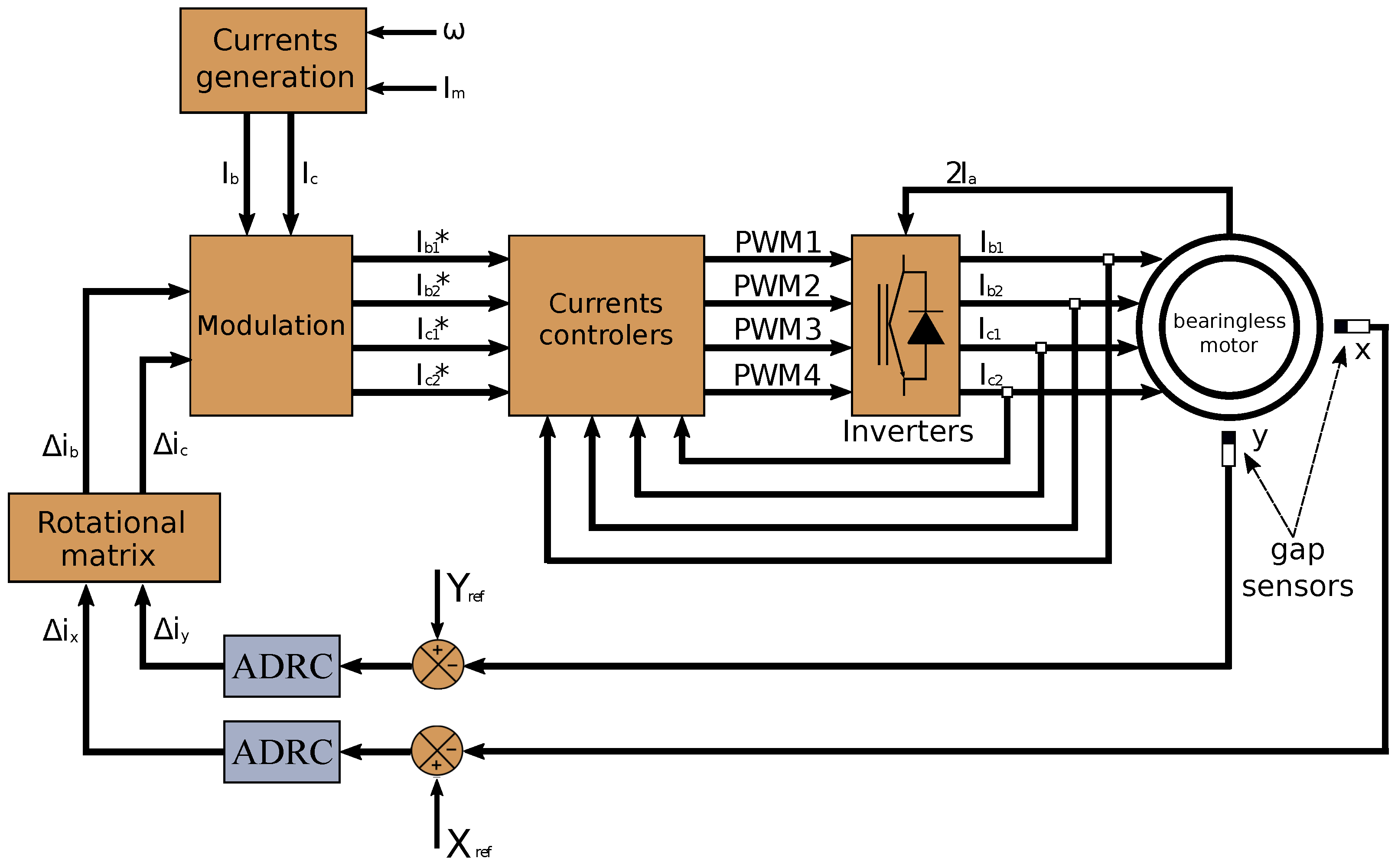
In this paper, the ADRC control technique is applied with two different structures to the control of a bearingless induction machine, the first structure uses linear estimation while the second uses nonlinear estimation. The results obtained show the dynamic behavior of the system output and states for the two versions.

2.1. Operation Principle

In the bearingless split winding induction machine, the electric currents in the stator and rotor coils generate magnetic fields that interact with each other. As a result of this interaction, forces arise that act on the rotor promoting its rotation and radial positioning. In the stator of the three-phase bearing motor, there are three divided groups of windings, each phase being displaced by ${120}^o$ relative to the others. With this distribution, it is possible to control the radial positioning of the rotor in all directions from the composition of the radial forces generated. Figure 1 shows the position of the windings relative to the X and Y axes.

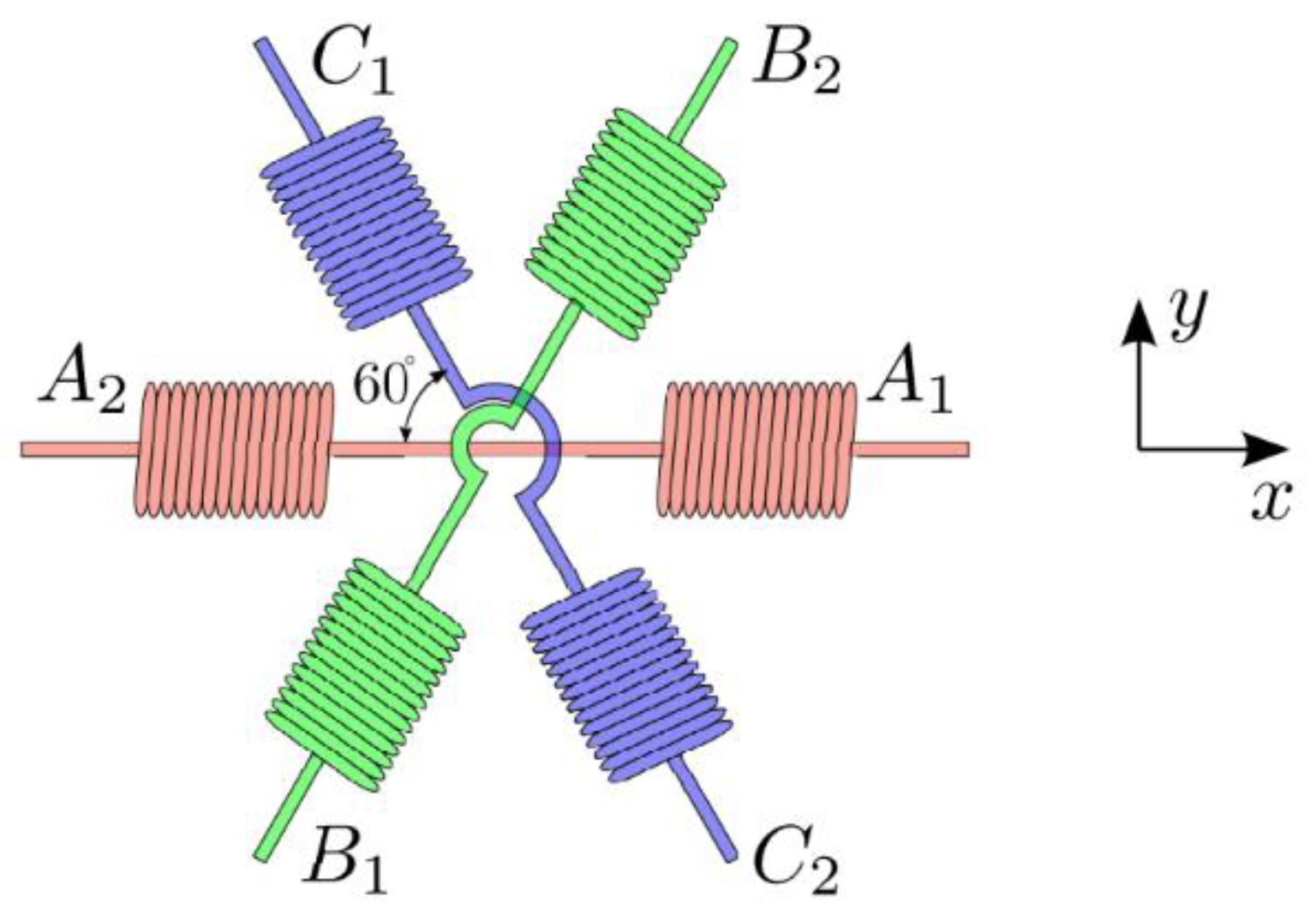
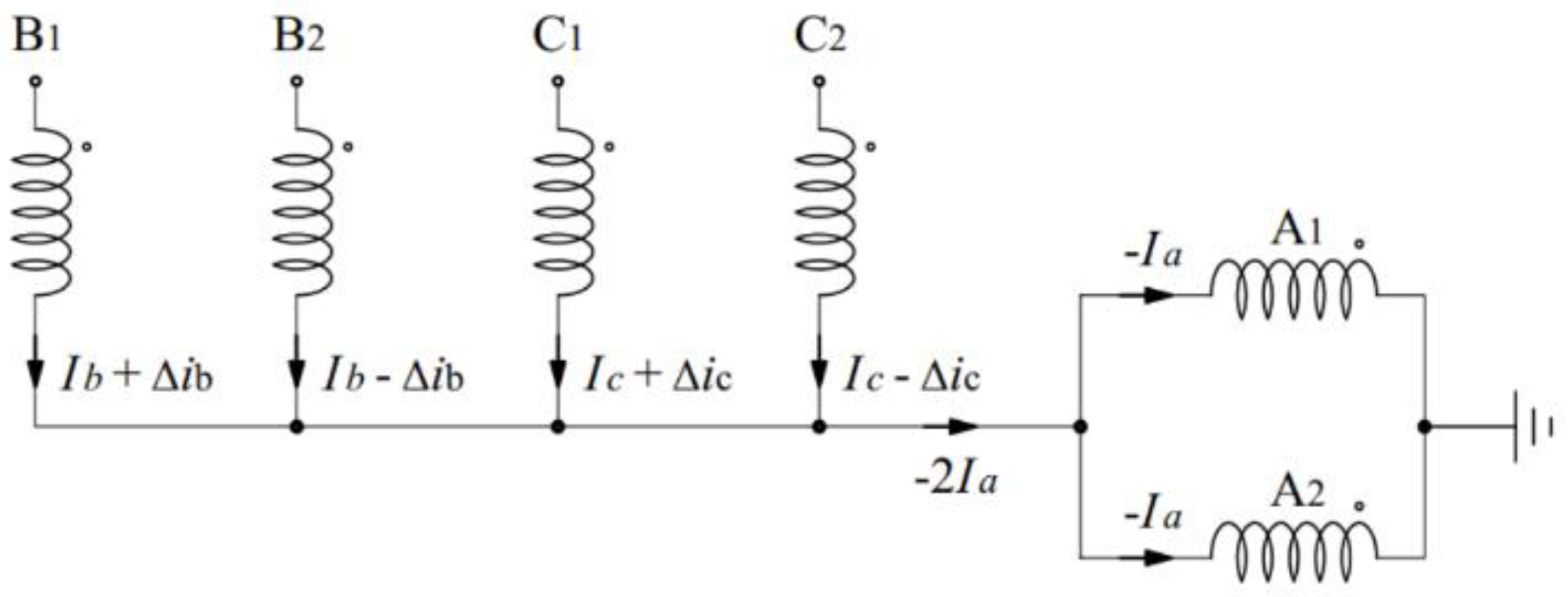
In the optimization proposal by [10] the coil connection arrangement was modified to the structure shown in Figure 2. This modification reduced the number of control and drive components for the currents in each phase.

Considering the currents ${\mathrm{I}}_b$ and ${\mathrm{I}}_c$ are given respectively by:

$$\begin{array}{c}\hfill I_b=I_{m}cos(\omega t-\frac{2\pi }{3})\\ \hfill I_c=I_{m}cos(\omega t+\frac{2\pi }{3})\end{array}$$

(1)

The sum of these currents, for the circuit in Figure 2 results in:

$$\begin{array}{c}\hfill I_b+I_c=I_{m}cos\left(\omega t\right)\end{array}$$

(2)

Since $I_b+I_c=-I_a$, it can be seen that for the modification performed by [10], the characteristics of the coil currents of phase A have been preserved.

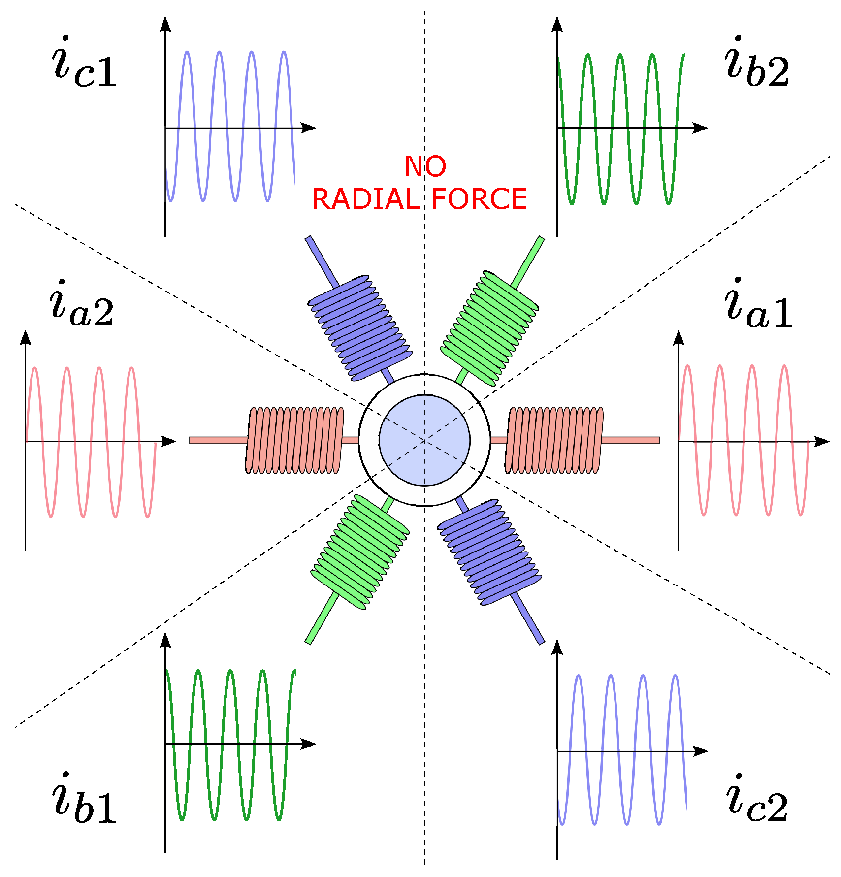
To illustrate the behavior of the currents per phase in the split-wound three-phase induction machine driven by a 4-arm inverter. Figure 3 shows the waveforms of the currents in each phase for the situation where the rotor is centered on the air gap. When the rotor is centered the modulation components are zero, therefore the phase currents have the same modulus $I_a=I_b=I_c$.

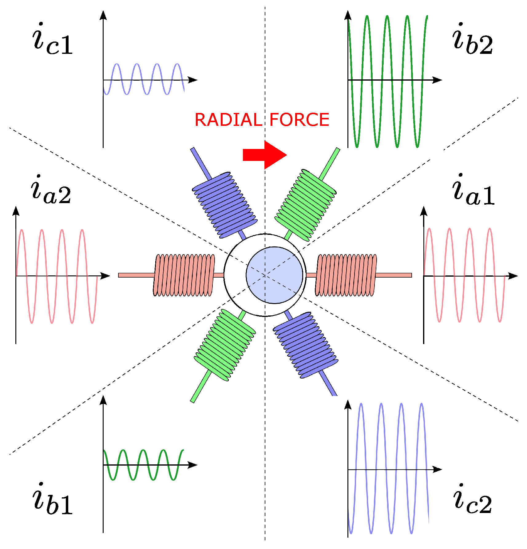
When unbalance occurs in one of the modulation components or disturbances that tend to move the rotor radially, the phase currents are altered by the control system in order to generate radial forces that bring the rotor back to the center of the stator.

Figure 4 shows the behavior of the currents during radial force generation to the right. To move the rotor shaft in the indicated direction, the control system must increase the currents of coils ${\mathrm{B}}_1$ and ${\mathrm{C}}_2$, and reduce the currents of coils ${\mathrm{B}}_2$ and ${\mathrm{C}}_1$.

3. ADRC Control

Modern control theory is focused on the time domain and can be applied to systems with multiple inputs and outputs, linear and nonlinear systems, and time-varying and time-invariant systems. One of the difficulties of modern state feedback control systems is that some variables are not accessible by measurement. In this sense, the concept of state observer becomes very useful to reconstruct non-measurable state variables from measurable variables. The Active Disturbance Rejection Control technique uses state observers to estimate in real-time the disturbances involved in the controlled process and then uses this information to obtain a good disturbance rejection capability [11]. 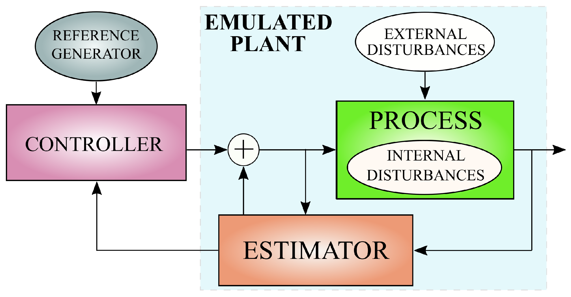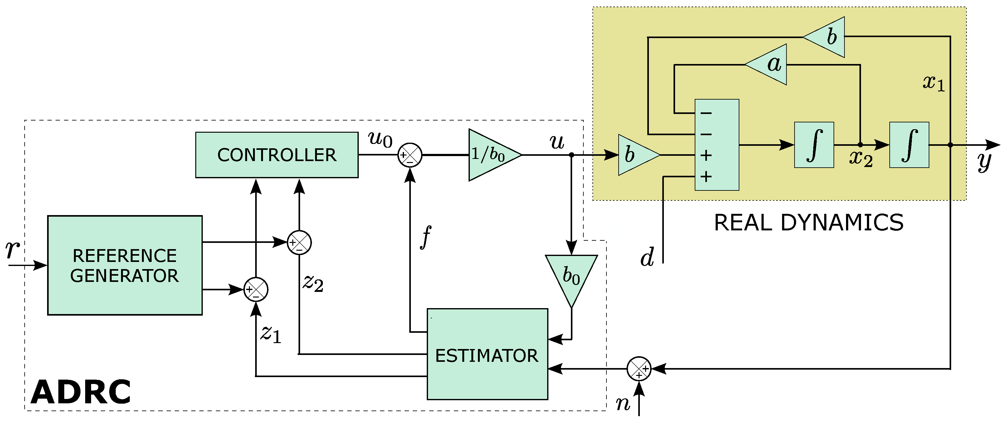In [12] ADRC control was proposed as a two-degree-of-freedom controller, with an inner loop for state estimation and disturbance rejection and an outer loop for controlling the process output dynamics. This structure is implemented based on three blocks, a reference generator, responsible for generating a smoothed version of the input signal and its derivatives, an estimator, responsible for estimating the process states and all the dynamics that differentiate it from a simple integrator system, and the control law, which subtracts from the original control the dynamics estimated by the observer. Figure 5 presents the general idea of the operating principle of an ADRC controller.

Considering a second-order process with representation in the state of states given by

$$\begin{array}{ccc}\hfill \ddot{y}& =& -a\dot{y}-by+w+bu\hfill \end{array}$$

(3)

y is the output; u is the input; w represents an external disturbance; a and b are system parameters. An approximate value of the disturbance b is the information needed for the ADRC implementation. Considering that there is no measurement available it is possible to approximate its value according to (3)

$$\begin{array}{c}\hfill \ddot{y}=-a\dot{y}-by+w+(b-b_0)u+b_{0}u=f+b_{0}u\end{array}$$

(4)

The term f in expression (4) is called the generalized disturbance and its value is given by $f=-a\dot{y}-by+w+(b-b_0)u$. The generalized disturbance is capable of encompassing a wide range of uncertainties and effects, such as: combined external and time-varying disturbances, unmodeled internal dynamics, nonlinearities, and internal parameter variations.

Assuming $x_1=y$ and $x_2={\dot{x}}_1$, the second-order system of equation (4) can be represented in state space by:

$$\begin{array}{ccc}\hfill {\dot{x}}_1& =& x_2\hfill \\ \hfill {\dot{x}}_2& =& f+b_{0}u\hfill \\ \hfill y& =& x_1\hfill \end{array}$$

(5)

If the generalized disturbance f can be estimated, its effect can be removed from the dynamics of the controlled process using (6).

$$\begin{array}{ccc}\hfill u& =& \frac{u_0-f}{b_0}\hfill \end{array}$$

(6)

The ADRC control of the process represented in (4) is shown in Figure 6.

The generalized disturbance is capable of encompassing a wide range of uncertainties and effects, such as: external and time-varying disturbances, unmodeled internal dynamics, nonlinearities, and internal parameter variations. ADRC groups these uncertainties and effects and uses this information to remove the effects of this information from the process control.

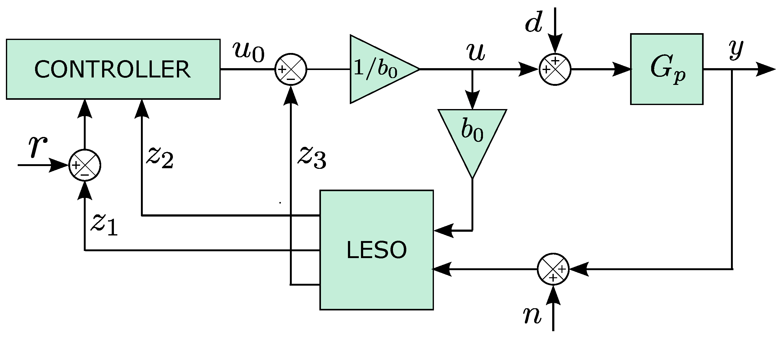
In [13] a linear structure for ADRC applied to second-order systems was proposed. The block diagram in Figure 7 shows the application of linear ADRC to a second-order $G_p$ system.

The output y is controlled by a LADRC from the application of input r. The states estimated by the linear extended state observer (LESO), are given by $z_1,z_2$, and $z_3$. The parameter $b_0$ is a tuning parameter. The external disturbances are represented by: d (input disturbance) and n (measurement noise).

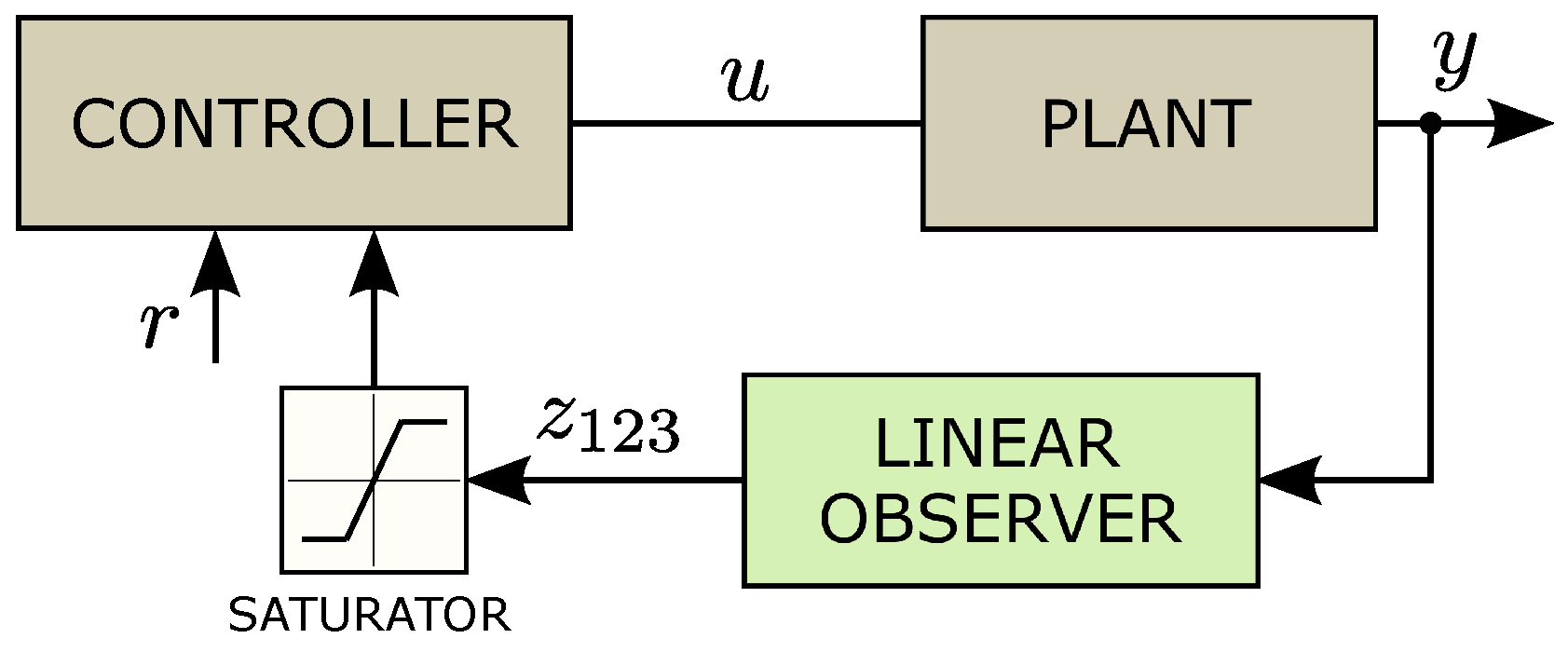
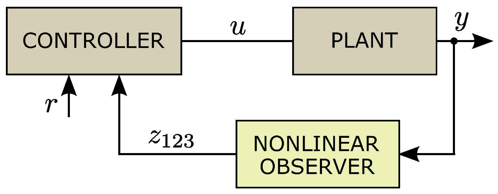
Keeping fixed the linear ADRC structure proposed in [13] this paper analyzed the application of two extended state observer structures. The first structure uses a linear observer with saturator at the output as shown in Figure 8. This structure mitigates the effects arising from the high error values between the estimated states and their actual values. The second structure uses nonlinear extended state observer as shown in Figure 9. This structure makes it possible to observe the influence of adding the nonlinearities on the dynamic performance of the system.

4. Description of the System

4.1. System Overview

Figure 10 provides an overview of the bench. The equipment has been grouped into the following blocks: monitoring and control, drive, and bearingless machine.

The bearingless motor block consists of the bearingless electric induction machine on which the tests were performed. The drive block comprises the entire infrastructure of electronic components and equipment responsible for providing the power supply at the appropriate levels to control the machine variables. The monitoring and control block consists of the electronic circuits, processors, and monitoring devices that were necessary to implement the system’s control and supervision routines. The variable $i_{abxy}$ represents the four-phase electrical connections that allow the drive block to supply controlled electrical currents to the bearing motor. The figure also indicates the reading of these $i_{abxy}$ currents performed by the monitoring and control block. The variable ${\Delta }_{xy}$ represents the signals corresponding to the radial positions of the x and y axes of the bearing motor read by the monitoring and control block. Finally, the orange arrow named PWM indicates the signals sent by the monitoring and control block to the drive block.

Figure 11 shows a real image of the experimental bench. This structure is located in the Actuation and Control Systems Laboratory in the Computer and Automation Engineering Department at UFRN.

4.2. Split-Winding Bearingless Machine

The prototype used works vertically with the goal of simplifying radial position control. The machine’s rotor is supported in the axial position by a mechanical bearing that is also responsible for fixing the machine’s lower end. Figure 12 shows the prototype.

The electrical data of the machine is detailed in Table 1.

4.3. Sensors

Two types of sensors are used on the bench: displacement sensors and current sensors. The displacement sensors detect the variation of the radial position of the machine shaft and the current sensors detect the phase currents reaching the machine.

4.4. DSP TMS320F28335

The DSP $TMS320F28335$ is a digital signal controller that has characteristics of a conventional processor because it contains in its structure circuits capable of executing programs stored in memories and also has additional circuits for digital signal processing, which includes hardware with special architecture and instructions for mathematical calculations and are able to perform real-time operations. In addition, the $TMS320F28335$ has in its structure memory and programmable input and output components, which makes the $TMS320F28335$ also a microcontroller.

4.5. Control Algorithm Implementation

The block diagram in Figure 13 shows the blocks needed for the practical experiments with the system. With the exception of the inverter block, all other blocks were implemented in C language in the DSP programming interface.

The general idea of the control algorithm is the existence of two cascaded control loops: the current control loop, with fast dynamic response and with the objective of making the currents in the controlled phases follow the specified reference; and the position control loop, which has slower dynamics than the current control loop and operates in a more external way, generating the references for the current control loop. The position control loop aims to maintain the radial position at the reference values $Y_{ref}$ and $X_{ref}$, for this, the position control signals are added to the magnetization currents $I_m$ to generate the necessary currents for the positioning of the rotor radial. The bias current block is responsible for generating via software the magnetizing currents of the machine. This block implements equations 1 and its arguments are the angular velocity and the peak value of the magnetizing currents. In the control algorithm, there are two ADRC blocks, one for each radial positioning axis of the machine. These blocks implement all the blocks required in the structure of the ADRC technique. These blocks receive the error calculated from subtracting the radial positions of the rotor by its references $Y_{ref}$ and $X_{ref}$ and perform the necessary operations to generate the correction signal ${\Delta }_{i}y$ and ${\Delta }_{i}x$. The rotational transformation block converts the control signals calculated in the x-y positioning referential to b-c corresponding to the spatial alignment of the controlled motor-mani fold coils. The function of the modulation block is to perform the composition of the rotation currents $I_b$ and $I_c$ with the control signals ${\Delta }_{i}b$ and ${\Delta }_{ic}$ and thus generate the references $I_{b1}^{*},I_{b2}^{*},I_{c1}^{*}$ and $I_{c2}^{*}$. Finally, the current control block implements four digital PI controllers, which monitor the machine currents and generate the PWM control signals for driving the inverters.

5. Experiments and Results

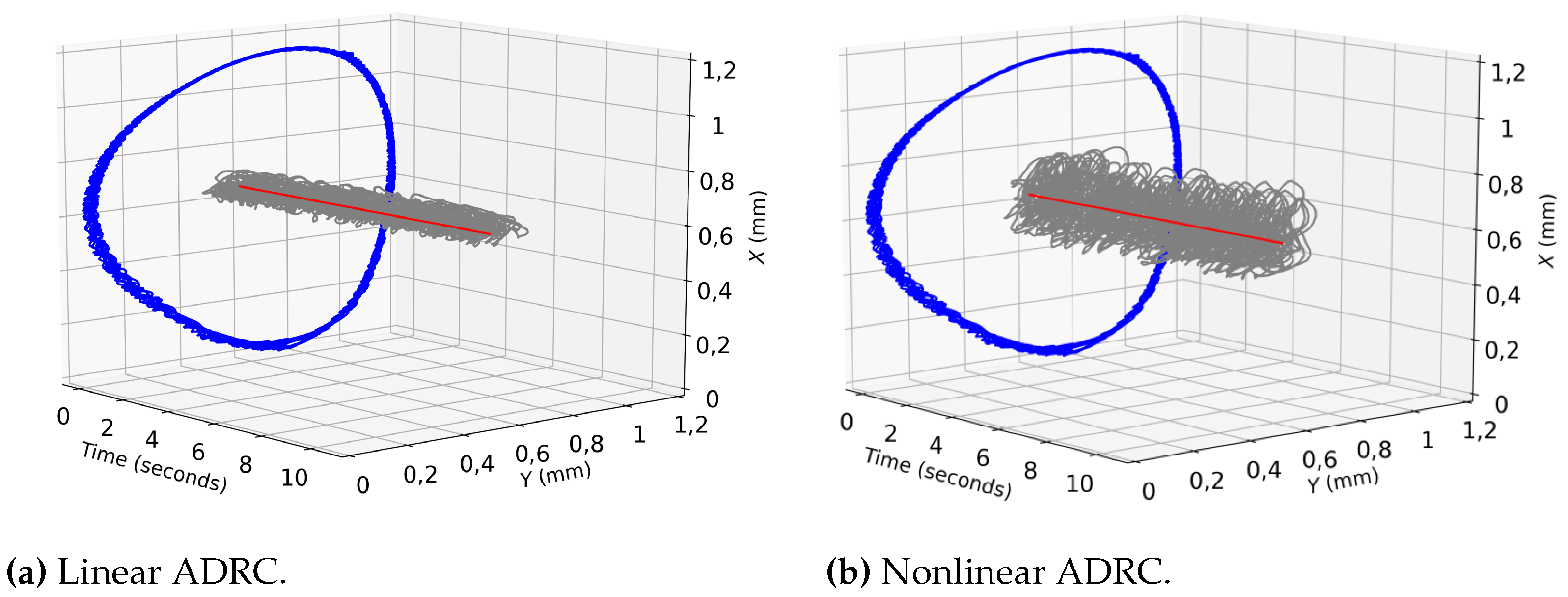
Two versions of ADRC controllers have been implemented in the $TMS320F28335$ DSP. The first one used the linear form proposed by Gao (2003) for the extended observer and the PD controller. The other version used fal-type nonlinearities in the observer structure. The results in three dimensions for the two implemented controllers can be seen in Figure 14a and 14b.

Figure 14a shows the behavior of positions X and Y in steady state for the first version of the controller. A mean error of $-1.17\%$ with a standard deviation of $0.03$ mm was obtained for the X axis. As for the Y-axis, an average error of $0.76\%$ with a standard deviation of $0.05$ mm was obtained. Figure 14b shows the behavior of the X and Y positions in a steady state for the version with nonlinearities. The mean error for the X-axis was $-0.09\%$ with a standard deviation of $0.07$ mm. For the Y axis, the mean error was $-0.05\%$ with a standard deviation also of $0.05$ mm. The results indicate the effect of adding non-linearity on the observer’s structure. It was possible to improve the regime error with the non-linear versions, but the variation around the reference became more evident, indicating an increase in the aggressiveness of the controller response.

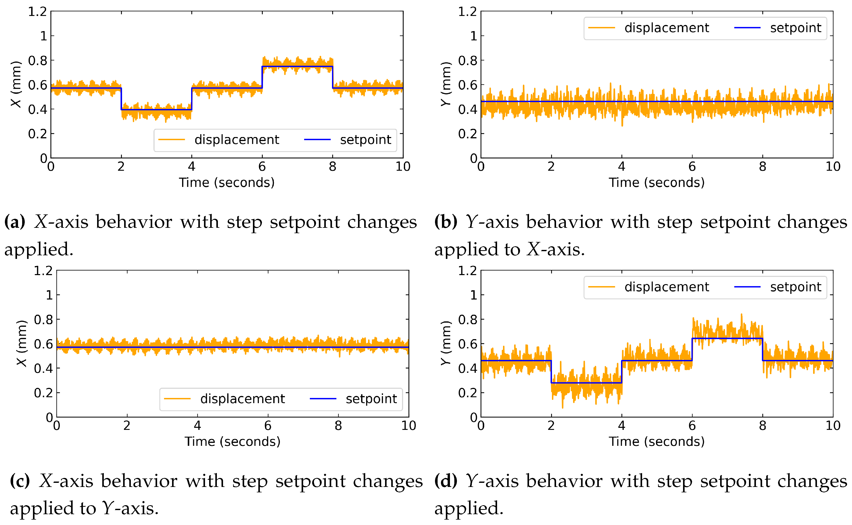
Figure 15a,b shows the behavior of the radial position signals when there are step-type reference variations in the X-axis only, keeping the Y- axis reference fixed, and Figure 15c,d when step-type variations occur in Y, keeping the X-axis reference is fixed.

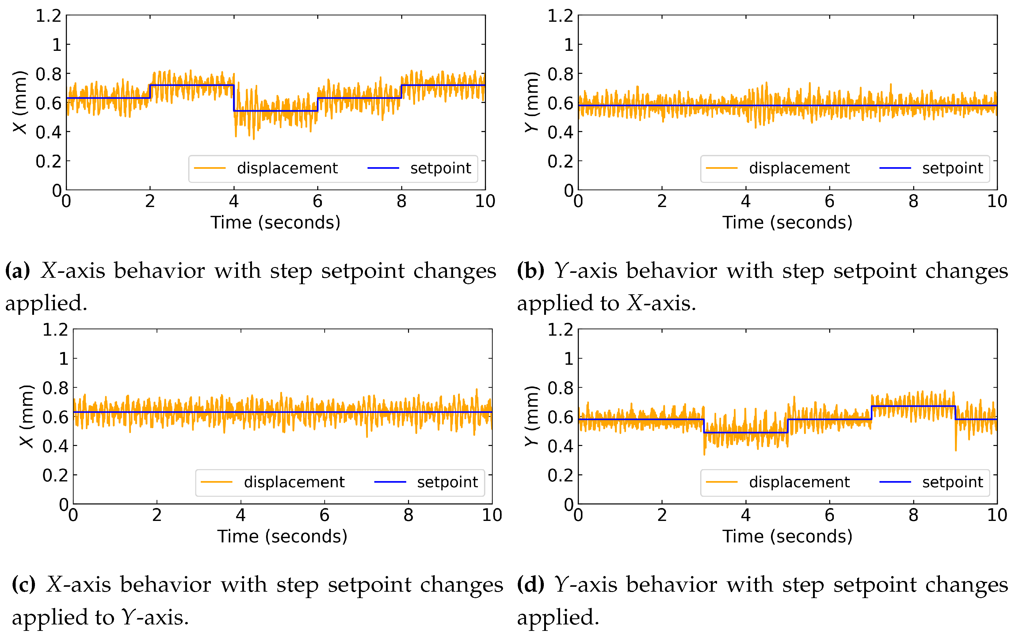
The results in Figure 15 show that step variations in one of the axes do not result in a significant influence on the dynamic behavior of the opposite axis. Variations in the axes were also performed for the controller with a non-linear observer. The results also indicate that there is a decoupling in the dynamic behavior of the radial position between the two axes.

The same test was performed to the controller with nonlinear observer. The results are showed in Figure 16.

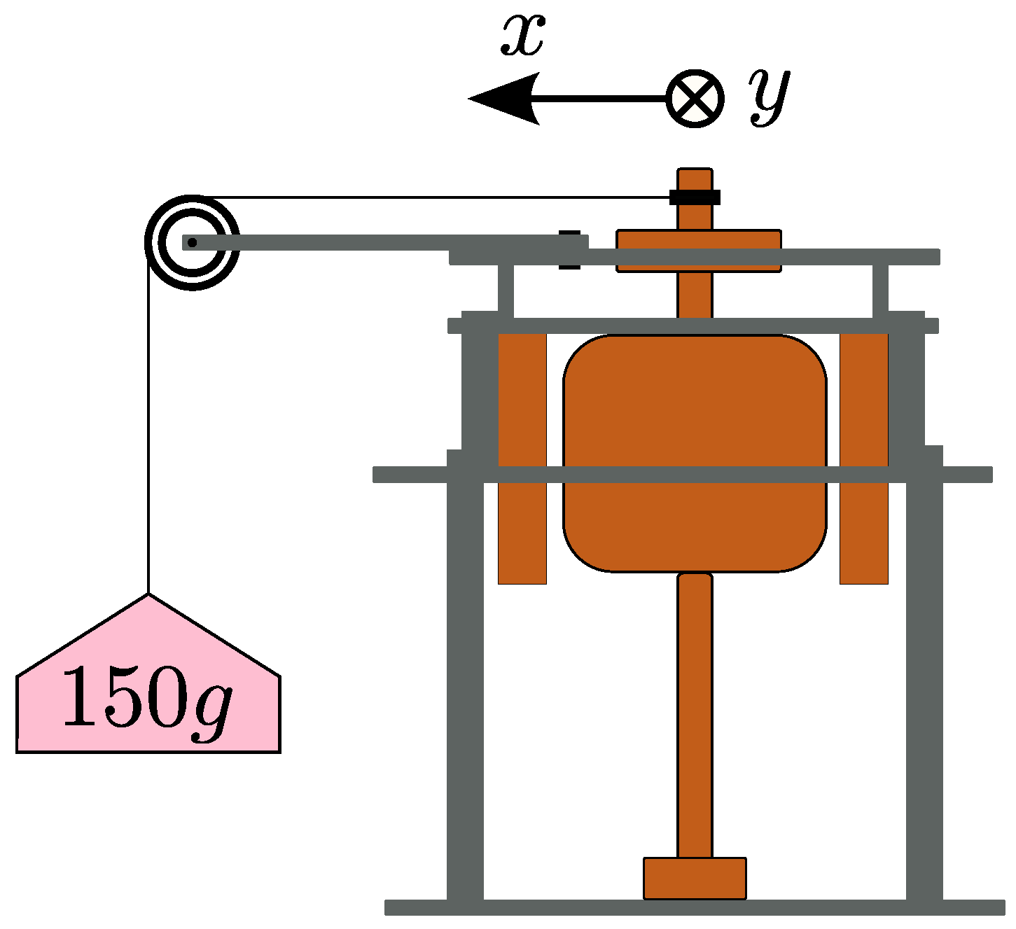
The addition of a radial load to the machine shaft in operation is an important analysis since this load is seen by the position controllers as an external disturbance in the form of a step. Therefore, it is a simple way to impose a perturbation and analyze the robustness of the controller in situations like this. For this analysis, an apparatus that allowed the addition of a radial load aligned with the X-axis was used. Figure 17 illustrates how the device was used to add the radial disturbance.

Figure 15. Response of radial position control under step setpoint changes for Linear ADRC.

Figure 15. Response of radial position control under step setpoint changes for Linear ADRC.

Figure 17. Illustrative image of the machine subjected to load addition.

Figure 17. Illustrative image of the machine subjected to load addition.

For each controller, the $z_1$, $z_2$, and $z_3$ states of the X and Y axes were collected in a time interval that allowed detecting the exact instant of addition of the radial load to the machine axis. Figure 18 and Figure 19 show the behavior of the states of the X and Y axes for the four implemented controllers. In each graph, a green dashed vertical line was inserted to indicate the instant the application of 150 grams of radial load aligned to the X-axis. This load was inserted so that the radial effort was applied in the positive direction of the axis. Figure 18a,b show the state behavior of the linear controller. Visually, it is possible to state that there was a certain degree of rejection of the radial disturbance, but it is evident that the regime error of the X-axis increased after the moment of application of the load. The Y-axis remained stable. It is not possible to perceive variations in the $z_3$ state on the scale used because the linear controller was implemented with saturators at the observers’ output in order to avoid the Peak phenomenon.

Figure 16. Response of radial position control under step setpoint changes for Nonlinear ADRC.

Figure 16. Response of radial position control under step setpoint changes for Nonlinear ADRC.

Figure 18. Estimated states behavior for Linear ADRC under radial load application.

Figure 18. Estimated states behavior for Linear ADRC under radial load application.

Through the analysis of the $z_1$ states of Figure 19a,b it is possible to conclude that the ADRC controller with NESO was less influenced by the application of the radial load in the steady state since qualitatively the response was very similar for the intervals before and after the addition of the disturbance. The behavior of the states indicated an aggressive reaction of the controller in the transient regime, resulting in high values of $z_2$ during this region of the collection. The change in the mean value observed for the $z_3$ state indicates that this variable was able to identify the addition of the external disturbance. the good rejection of the observed perturbation may be a result of this. Quantitatively, the results of Figure 18a,b and Figure 19a,b can be summarized according to Table 2. Table 2 shows the average values in a steady state of the observed states.

Figure 19. Estimated states behavior for Nolinear ADRC under radial load application.

Figure 19. Estimated states behavior for Nolinear ADRC under radial load application.

The value of the $z_1$ state for the linear controller indicates that there was a displacement of the mean value of the output after applying the load. This is a limitation of the linear observer as its states need to read limited in amplitude to avoid peak phenomenon and guarantee stability. As indicated by the value of $z_3$ after applying the load, it was blocked in the imposed saturation. The saturation of state outputs impairs the ability to reject disturbances. The mean value of the $z_1$ state of the non-linear indicates that it was able to reject the load addition. Furthermore, the significant change in the value of $z_3$ shows that it was able to identify the disturbance.

The value of $z_3$ in Table 2 becomes more negative after adding the load because the control loop error is given by:

$$\begin{array}{c}\hfill Error=pos-ref\end{array}$$

(7)

that is, when the radial position is displaced from the reference value in the sense of increasing the error value, the control signal must increase in order to restore the equilibrium position close to the reference. Knowing that the control signal is calculated by:

$$\begin{array}{ccc}\hfill u& =& \frac{u_0-z_3}{b_0}\hfill \end{array}$$

(8)

it means that the more negative the value of $z_3$, the greater the values of the control signals and the greater the control effort in the sense of rejecting the action of the disturbance in the system output. The more positive the displacement value is in relation to the reference, the greater the control signal must be.

Finally, to analyze the relationship between the value of $z_3$ and the intensity of the radial disturbance applied to the motor shaft and also to verify to what extent the system could reject the radial load, masses of 32 grams were added one by one in the application support of the load. This test was performed with the NESO-based controller only. In the first step, the radial load support was aligned on the X-axis and then on the Y-axis. For each added mass, the regime errors of the X and Y positions were calculated and the $z_3$ states were collected. The results are shown in Figure 20a,b and Figure 21a,b. Figure 20a,b show the results for the radial load bearing aligned with the X-axis.

Figure 20a shows that the regime error remained close to zero for loads of up to 224 grams. When the radial load increased to 256 grams, the position control in the X-axis became unstable but remained stable on the Y-axis. Figure 20b shows the estimation of generalized disturbances for the X and Y axes increase in load and the $z_3$ state of the X-axis. This variable becomes more negative as the load increases, as expected. Figure 20b also shows that the load added in the X direction also influenced the $z_3$ state of the Y axis. This indicates that the load support was not perfectly aligned with the desired axis, or that the X and Y sensors could not have been perfectly spaced 90 degrees apart. Figure 21a and 21b show the same analysis, this time for the radial load added in the positive direction of Y. The Y axis showed a lower radial disturbance rejection capacity since it only managed to keep the regime error close to zero up to 160 grams of load. The Y-axis control became unstable for the 192-gram load, while the X-axis remained stable for all analyzed loads. Figure 21b indicates that there is also an approximately linear relationship between the value of $z_3$ and the value of the added charge. Likewise, there was a smaller scale detection of radial disturbance by the $z_3$ state of the X-axis. In this test, the influence on the cross-axis was greater. The results of the load curve for both axes showed that there is a linear relationship between the perturbation and the $z_3$ state. This relationship is fundamental to the success of the strategy and indicates that the extended state observers are capable of detecting external disturbances without the need for physical sensors installed in the process.

6. Conclusions

In this paper, the application of the ADRC active disturbance rejection technique to a bearingless induction machine was analyzed. During the laboratory tests, two structures for the extended state estimator were used, a linear structure and a nonlinear structure. The results for step reference variation, for both versions, show good dynamic decoupling between the radial displacements in the X and Y axes. The test with load imposition showed that both observers were able to detect the generalized disturbance, however, only the nonlinear observer was able to maintain the same average system output value before and after load application. The results obtained show the success of the ADRC technique in the active estimation and rejection of disturbances in the radial positioning process of a split rotor bearingless machine. The results also show the higher active rejection capability of the technique applied with a nonlinear observer since with this type of observer disturbances of this nature are estimated and compensated.