1. Introduction
The alum sludge (also red mud or bauxite tailings) is a byproduct of the drinking water treatment process alum [
1]. In recent decades, several studies have examined the use of alum sludge as a soil stabilizer [
2]. As a soil stabilizer, alum sludge has the main advantage of improving the soil’s physical properties, such as strength and stability [
3]. The reason for this is that alum sludge contains high levels of alum, which reacts with the soil to form a solid and stable structure [
4]. As a result of this reaction, soil density and compaction increase and improving soil stability and reducing erosion sensitivity [
4]. But also, for pure aluminum sludge stability gained by adapted scheduling of bauxite tailings is critical to warrant safe tailings deposition [
5].
According to Nguyen et al. [
4], alum sludge as a soil stabilizer reduces the soil’s flexibility and makes it less susceptible to deformation. This reduction in flexibility results in improved soil structure and increased stability [
4]. Also, in geotechnical side, Nguyen et al. [
4] showed that with increasing sludge to the soil, the undrained compression strength (UCS) of soil increased. In addition, several studies have demonstrated that alum sludge can be an effective alternative to traditional soil stabilizing agents, such as cement and lime [
6,
7,
8].
Alum sludge as a soil stabilizer can have several environmental advantages [
9]. The first benefit is that it reduces the amount of waste produced by the alum production process by recycling the sludge and reusing it for soil stabilization [
9]. Furthermore, alum sludge reduces the need for conventional soil stabilizers, which are often derived from non-renewable sources and may emit large amounts of carbon dioxide [
10]. In addition to improving soil stability, alum sludge can also improve soil chemical properties [
9]. Studies have shown that alum sludge can neutralize soil acidity and improve soil pH [
11,
12]. The importance of this is that soil acidity can inhibit plant growth and reduce crop yields [
11]. As a result, better water infiltration and retention occurs in the soil, which is essential for the growth and development of plants. Additionally, improving soil permeability can reduce soil erosion and contribute to improving soil health [
13]. Alum sludge is cost-effective when used as a soil stabilizer compared to traditional soil stabilizers such as cement, coal and fly ash [
14].
As a soil stabilizer, alum sludge has been shown to have varying efficiency depending on the type of soil and the conditions of its application. As an example, clay soils are naturally active, so the use of alum sludge may greatly benefit them [
15]. Similarly, the effectiveness of alum sludge as a soil stabilizer can be affected by environmental factors such as temperature, humidity, and rainfall [
16]. Studies showed that it is important to consider the specific soil and environmental conditions when using alum sludge as a soil stabilizer [
16,
17].
In the history of studies, various factors have been identified as influencing the behavior of sludge. There are several parameters to consider, including soil and sludge density, specific gravity of soil, liquid limit and plasticity of soil, sludge content etc. The multiplicity of parameters and the non-linearity. It would be necessary to predict performance using an equation with a large number of parameters that would require quantification, which does not exist. In the last two decades, artificial intelligence (AI) methods have been used to resolve this issue. Using artificial intelligence techniques, it is possible to determine the relationship between different parameters with a high degree of accuracy without prior knowledge. Various topics in geotechnical engineering, such as slope stability [
18,
19,
20], tunnelling [
21,
22,
23], pavement and road construction [
24,
25], soil cracking [
26,
27,
28], rock mechanics [
29,
30], soil dynamics [
31,
32,
33,
34] and soil stabilizers [
35,
36,
37] have been addressed using artificial intelligence methods [
38]. Nevertheless, only two studies have used artificial intelligence to predict properties from mixing sludge with soil [
39,
40]. Aamir et al. [
41] used a small database of 18 datasets to predict the CBR parameter using artificial neural network (ANN). A high
R2 of 0.99 was observed as well as a small RMSE of 0.057. Similarly, Shah et al. [
39] used a 21-sets database and artificial neural network (ANN) method to predict the CBR of mixtures of sludge and soil. The results of the study were very promising with a
R2 of 0.97 and an RMSE of 0.58. However, the big gap is that both studies used only one classic artificial intelligence method, ANN, and grey box methods were not employed. Grey box methods are those methods that have an output like a tree or an equation. Also, the used databases were relatively small, which may limit the range of values of the parameters.
In order to fill these gaps, this study uses two black-box AI methods, namely artificial neural network (ANN) and super vector machines (SVM), as well as a grey-box AI method, namely genetic programming (GP), in order to predict CBR. By using this approach, both black-box and grey-box models will be examined. The ANN method that is currently used as standard will be compared with another black-box method, SVM. A database of 27 CBR test results on a variety of soil types was used for this purpose. Initially, there are nine input parameters from laboratory tests, whose number are discussed in detail. The sensitivity of the AI models as well as the importance of the input parameters has been evaluated.
2. Data-Driven Modeling
After analyzing the collected database, CBR was predicted using three artificial intelligence methods, including artificial neural network (ANN), genetic programming (GP) and support vector machine (SVM).
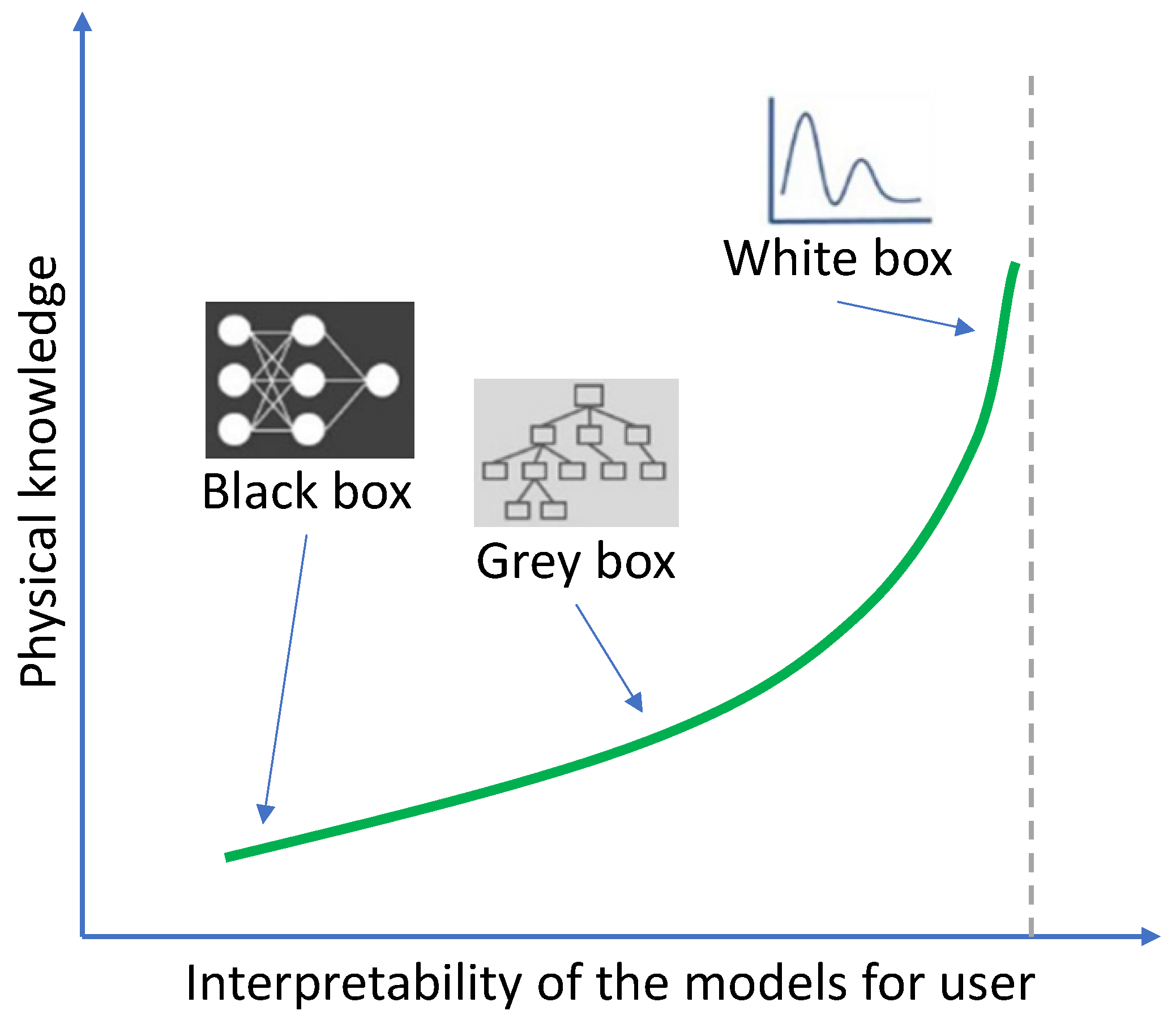
The use of AI algorithms for material characterization and design has been met with skepticism due to concerns about the reliability of their complex models. The lack of transparency and knowledge extraction processes in AI-based models is a major challenge. Mathematical modeling techniques can be categorized as white-box, black-box, and grey-box, depending on their level of transparency (
Figure 4). While white-box models are based on first principles and provide an explanation of the underlying physical relationships of a system, black-box models do not provide any feasible structure of the model. Grey-box models, on the other hand, identify the patterns between the data and provide a mathematical structure of the model. ANN is a popular black-box modeling technique widely used in engineering, but its weights and bias representation does not provide details about the derived relationships. GP is a newer grey-box modeling technique that uses an evolutionary process to develop explicit prediction functions, making it more transparent than other ML methods, especially black-box methods such as ANN and SVM. The mathematical structures derived by GP can be used to gain important information about the system performance.
Figure 4.
Classification of the AI modelling techniques (Adapted from Giustolisi et al. [
41] and Zhang et al. [
42]).
Figure 4.
Classification of the AI modelling techniques (Adapted from Giustolisi et al. [
41] and Zhang et al. [
42]).
2.1. Support Vector Machine (SVM)
In supervised learning model (SVM) method, initially developed by Vapnik [
43], weights are calculated based on input data, known as training data, in order to learn the governing function from a set of inputs. SVM selects a limited number of input sample vectors, which are always a fraction of the total number of samples. These input vectors are referred to as support vectors. Using these input vectors, parameter values of the method for minimizing error are calculated. As a result, SVM requires much less data than similar methods such as ANN, and as a result, it takes much less time and money.
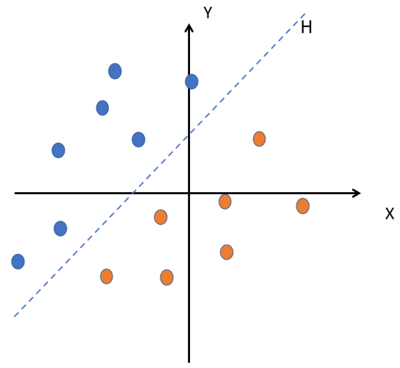
The goal of this method is to find a classifier that separates the data and maximizes the distance between these two classes.
Figure 5 shows a plane cloud that separates two sets of points.
Figure 5.
The hyperplane H that separates the two groups of points.
Figure 5.
The hyperplane H that separates the two groups of points.
According to
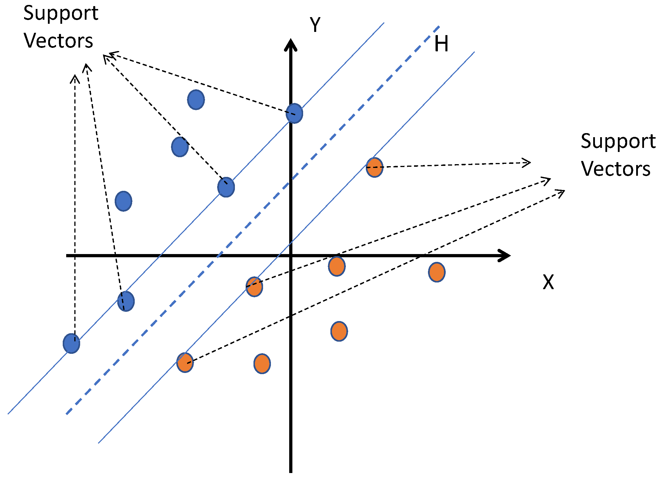
Figure 6, the closest points used alone to determine the hyperplane are called support vectors. As is clear, there are many hypermaps that can divide samples into two categories. The principle of SVM is to choose something that maximizes the minimum distance between the hypermap and the training samples (that is, the distance between the hypermap and the support vectors), this distance is called the margin.
Figure 6.
Support vectors.
Figure 6.
Support vectors.
Kernel function, as an important part of SVM method, receives data as input and transforms them into the required form. Various functions are provided for this purpose. Some of these functions, including linear, nonlinear, polynomial, radial basis function (RBF), and sigmoid, are given in equations 8 to 12. According to Equations 8 to 12, the kernel function is a series of mathematical functions that provide a window for data manipulation. With the help of this transformation, a complex and non-linear level of decision-making becomes a linear equation, but in a larger number of dimensional spaces.
where
xi and
xj are vectors in input space,
γ and
σ parameters define the distance influence of a single sample,
d is degree of polynomial,
c ∈
R is the relative position to the origin,
κ’ is a real-valued positive type function/kernel,
α,
T and
c are certain values.
In this study, two important functions, i.e., radial basis function (RBF) and Gaussian kernel, which have been successful in past research, were evaluated along with two other functions, i.e., Sigmoid kernel and Polynomial kernel functions.
2.2. Artificial Neural Network (ANN)
Artificial Neural Networks (ANNs) have a history that dates back to the mid-20th century when the mathematical model for the perceptron was first introduced by Rosenblatt [
44]. The development of the backpropagation algorithm in the 1980s by Rumelhart et al. [
45] improved the training of multi-layer ANNs and led to their widespread use in various fields. Since then, ANNs have continued to evolve with the development of new architectures and learning algorithms [
46].
The Artificial Neural Network (ANN) is a machine learning model that is based on the structure and function of the human brain [
46]. Artificial neural networks are composed of interconnected nodes or artificial neurons that process information and make predictions in response to inputs. By combining the inputs and the weights assigned to each connection, the interconnected nodes produce an output. There are a number of applications for artificial neural networks, including image classification, speech recognition, and natural language processing, among others. In the field of machine learning and artificial intelligence, they have proven to be effective at solving complex problems.
Due to their ability to learn from data and make accurate predictions or classifications based on that data, artificial neural networks (ANNs) have become one of the most powerful tools in the field of machine learning and artificial intelligence [
38]. As a result, they simulate the structure and function of the human brain, which is composed of many neurons connected by synapses.
Each node or artificial neuron in an ANN performs simple computations based on the input it receives and the weights assigned to the connections [
48]. One neuron’s output is then passed on as input to other neurons in the network, allowing the information to be processed and transformed multiple times before it is finally produced. Feedforward refers to this process of processing and transforming information through multiple layers of neurons.
There are various types of artificial neural networks, each designed for a particular task or application. The most popular types of ANNs include feedforward networks, recurrent networks, and convolutional neural networks [
49]. An ANN can be used for a variety of purposes, and each type has its own strengths and weaknesses.
As the most basic type of ANN, feedforward networks are used for simple tasks such as binary classification and linear regression. On the other hand, recurrent networks are used for sequences of data, such as speech or text, and are capable of capturing temporal relationships. An image or video analysis can be performed using convolutional neural networks, which are specifically designed to capture the spatial relations between pixels in an image or video.
Artificial Neural Network (ANN) can be used to model complex relationships with no established mathematical relationships [
49]. The ANN method is consisting of artificial neurons and is commonly used to fit nonlinear statistical data. For this purpose, ANN identifies the relationships between input and output parameters based on the strength of the connection between the two neurons, known as “weight”. Next, the network seeks to optimize the matrix of weights, which is achieved through practice and adjustment, which is called the paradigm [
51]. One of the strongest paradigms is the back-propagation paradigm. In this study, two back-propagation algorithms are used: (i) Levenberg-Marquardt (LM) algorithm [
52], and (ii) Bayesian Regularization (BR) [
53] algorithm.
Input, hidden and output layers are 3 main components of ANN architecture. In this study, for each algorithm, i.e., LM and BR, one, two, three, four and five hidden layers are considered. Log-sig and tan-sig are transfer functions within each neuron. In this study, 5 different architectures of ANN, with 1 to 5 hidden layers, were modelled for each algorithm. Furthermore, by trial and error, 45 neurons were considered for each hidden layer and each network 3 times is re-trained.
2.3. Genetic Programming (GP)
John Koza, a computer scientist and researcher at Stanford University, developed the first genetic programming system in the early 1990s. Using this system, he evolved computer programs capable of solving mathematical problems and controlling robots. Several genetic programming frameworks and toolkits were developed as a result of this development.
As a subfield of Artificial Intelligence and Evolutionary Computation, Genetic Programming (GP) is a method for solving complex problems using a process inspired by natural selection and genetics. In this approach, potential solutions are represented as trees of operations (also known as computer programs) and then improved using genetic algorithms.
The GP algorithm generates an initial population of computer programs at random and evaluates their fitness in accordance with a problem-specific objective function. Through genetic operators such as crossover and mutation, the best programs are selected to produce the next generation. The process continues until a satisfactory solution is found or a stopping criterion is met.
A wide range of problems can be solved using GP, including function approximation, symbolic regression, and even game play. There are several strengths of GP, including its ability to find complex solutions that are difficult or impossible to discover manually, as well as its ability to handle high levels of uncertainty and noise in the data. It can, however, be computationally expensive and may have difficulty finding solutions in a reasonable amount of time for very complex problems.
3. Database Collection and Processing
3.1. Experiment and Data Collection
The database was prepared based on the results of two studies [
4,
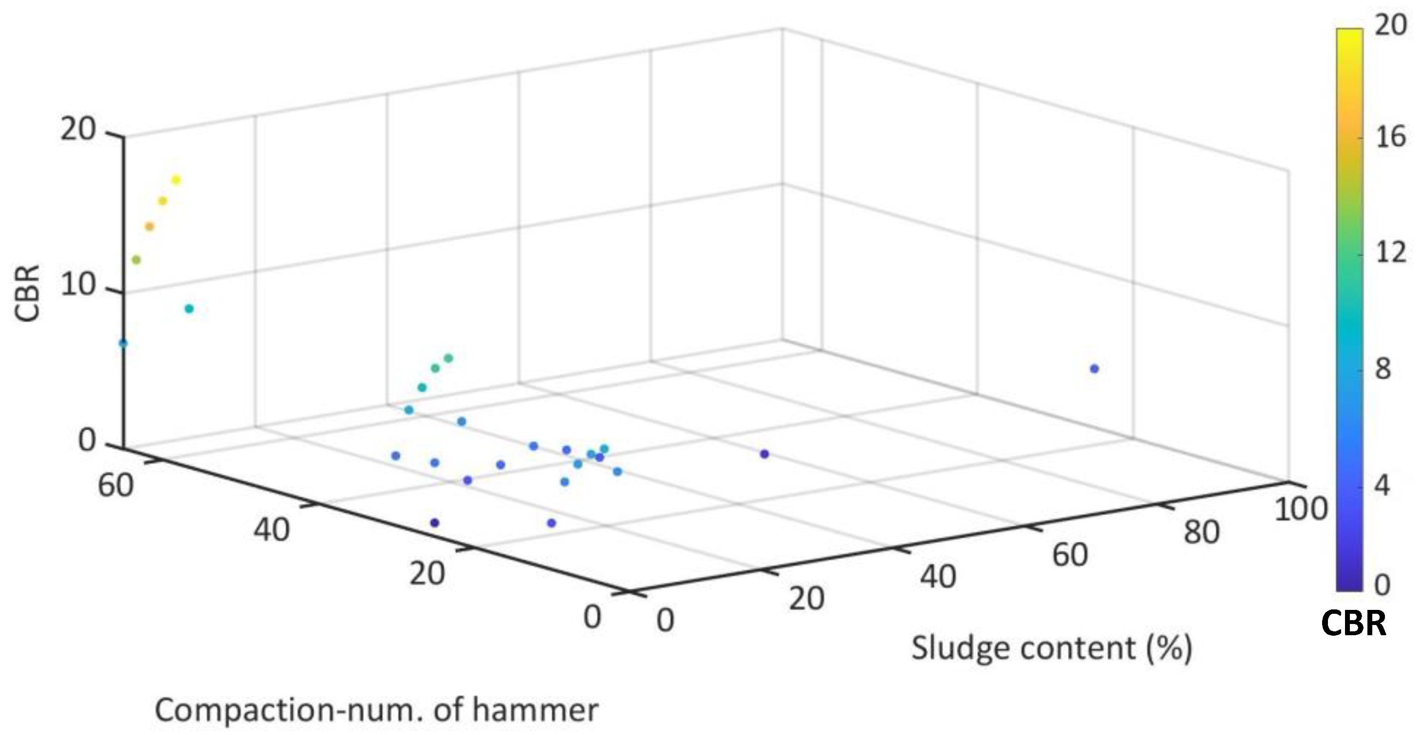
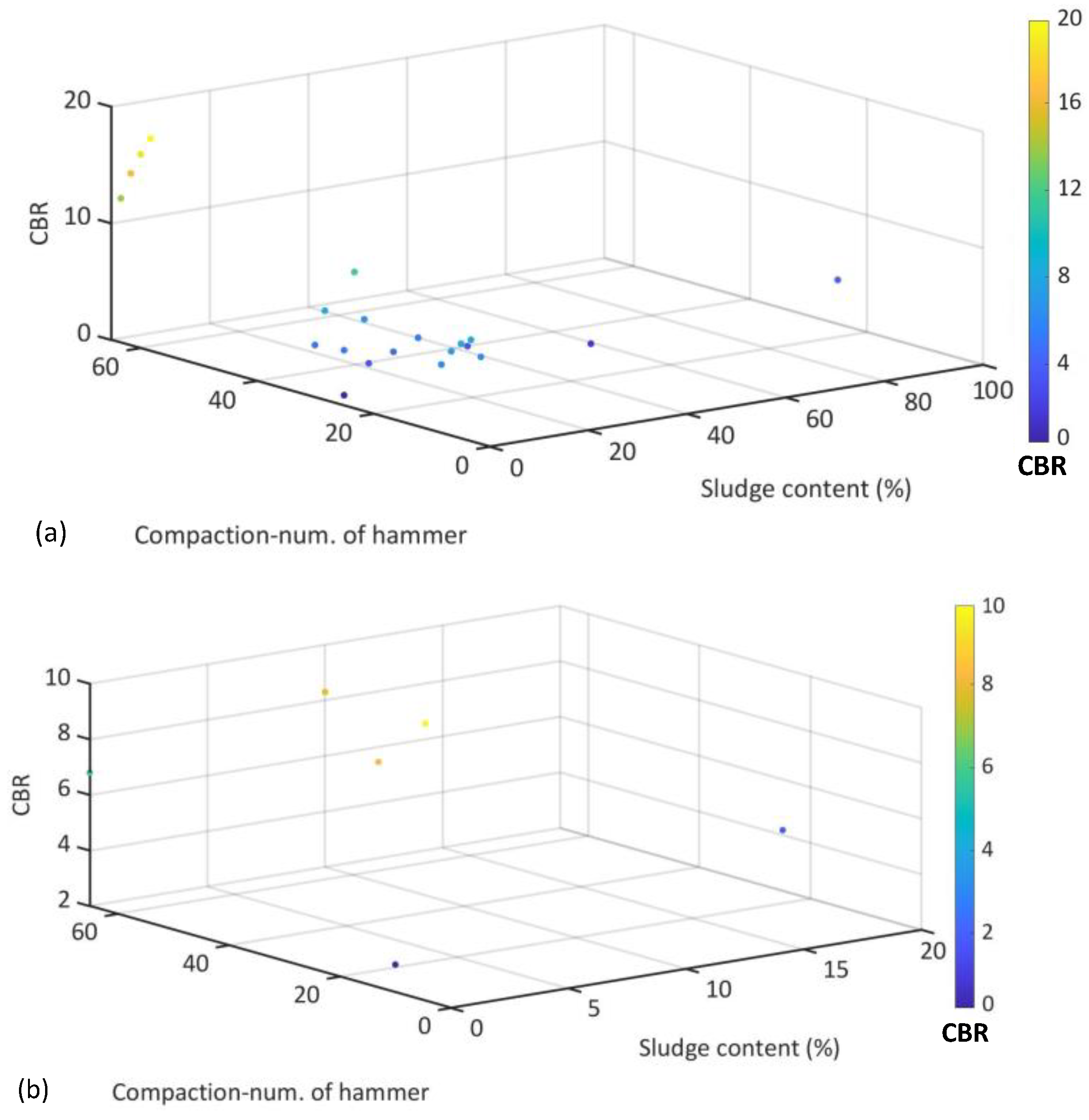
40]. A 3D representation of the collected database for CBR is shown in
Figure 1. The existing database considers nine input parameters, including liquid limit (LL) and plasticity index (PI) of soil, the sludge content, compaction number of blows, optimum moisture content (OMC) and maximum dry density (MDD) of soil and mixture and bulk modulus Gs of soil. CBR is the only output.
Figure 1.
Database used for modelling based on the CBR.
Figure 1.
Database used for modelling based on the CBR.
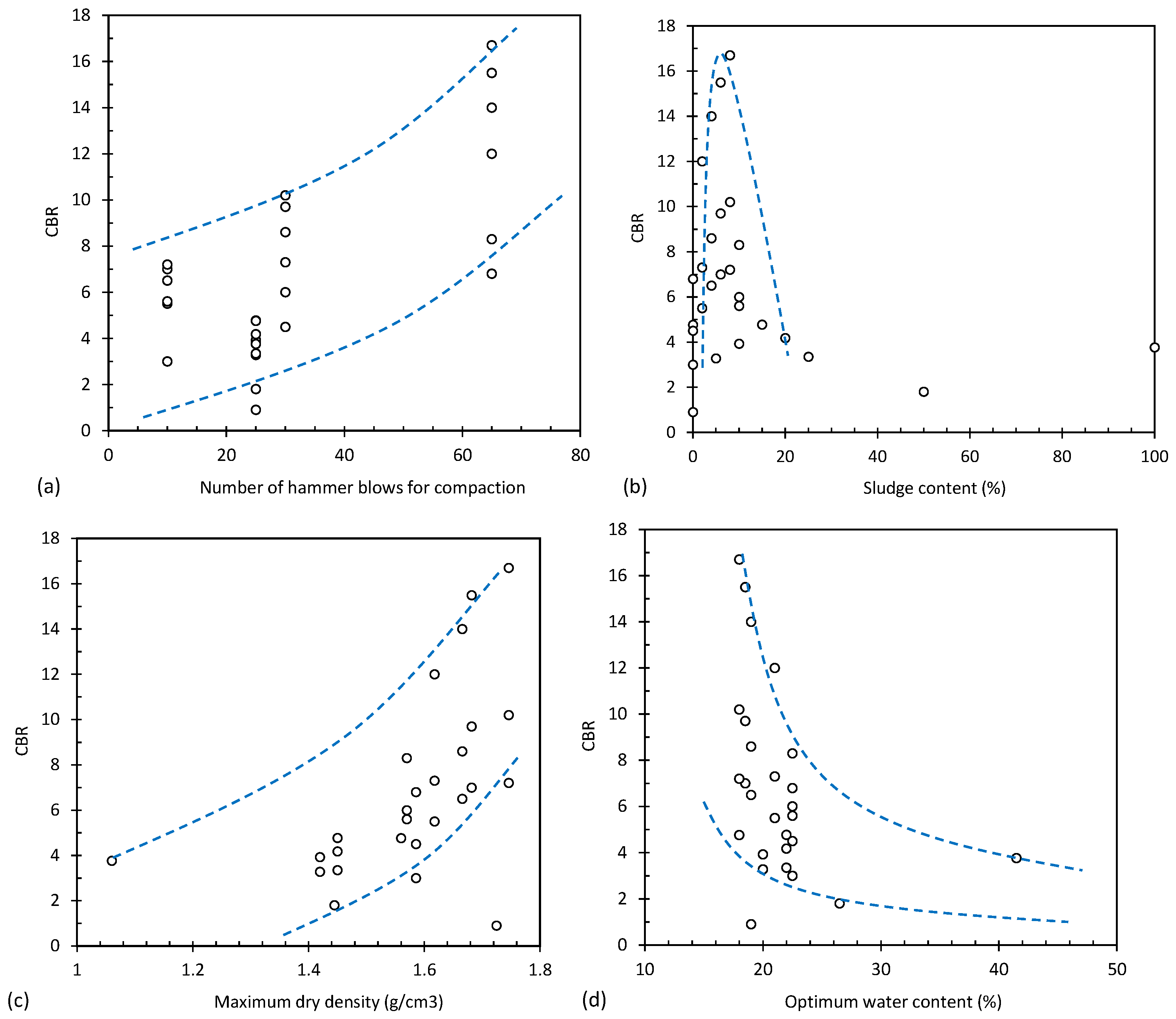
Figure 2 shows the effect of different input parameters, such as compaction number of blows, sludge content, maximum dry density and optimum water content, on CBR. According to the results in
Figure 2a, with an increase in the number of compression hammer blows, CBRs increased dramatically as the number of compression hammers increased.
Figure 2b illustrates the effect of sludge content on CBR. It can be seen from
Figure 2b that as the sludge content increased, CBR increased significantly at first. When the sludge content reached around 8%, CBR began to decrease as the sludge percentage increased.
Figure 2c shows the effect of increasing the maximum dry density (MDD) of the soil on the CBR of the soil. According to the results, it can be concluded that the CBR increased as the maximum dry density of the soil increased. In addition,
Figure 2d shows the effect of optimum moisture content (OMC) on CBR. Results depict that CBR decreased as optimum water content increased.
Figure 2.
Effect of (a) compaction number of blows, (b) sludge content, (c) MDD and (d) OMC on the CBR in collected database.
Figure 2.
Effect of (a) compaction number of blows, (b) sludge content, (c) MDD and (d) OMC on the CBR in collected database.
In order to provide a more detailed analysis of the database,
Table 1 shows the statistical information including the minimum, maximum, mean and standard deviation.
3.2. Preparation of the Data for AI Modelling
3.2.1. Normalization
In a database, each input or output variable has a specific unit. The data normalization function can eliminate the weight of the units, reduce network errors, and increase training speed by adjusting the data between zero and one. The linear normalization function utilized in this study is outlined below.
The four terms in this equation are Xmax, Xmin, X, and Xnorm, which correspond to maximum, minimum, actual, and normalized values, respectively.
3.2.2. Testing and Training Databases
There are two types of databases required for the implementation of mathematical models, namely training databases and testing databases. For all three mathematical models, training and testing were randomly divided.
Figure 3 shows the main division of the database, where 80% of the main database was used for training and 20% for testing.
A random database division resulted in two test and experiment databases that were considered fixed and were used in all three mathematical models. Statistical parameters are shown in
Table 2 and
Table 3, respectively, for the training and test databases. The statistical information, including the minimum, maximum, mean, and standard deviation, is very similar for both databases. This issue can increase the accuracy of the network in predicting the output.
Figure 3.
Distribution of (a) training and (b) testing databases.
Figure 3.
Distribution of (a) training and (b) testing databases.
3.2.3. Statistical Parameters
The performance of a network can be evaluated through a variety of parameters such as coefficient of determination (
R2) and mean absolute error (MAE). Equations 2-7 show the definitions of Mean Absolute Error (MAE), Mean Square Error (MSE), Root Mean Square Error (RMSE), Mean Squared Logarithmic Error (MSLE), Root Mean Squared Logarithmic Error (RMSLE), and Coefficient of Determination (
R2).
Where N is the number of datasets, Xm and Xp are actual and predicted values, and , are the average of actual and predicted values, respectively. Ideally, the model should have a R2 value of 1 and a MAE, MSE, RMSE, MSLE, RMSLE value of 0.
4. Results
4.1. Support Vector Machine (SVM)
In order to derive an optimal SVM model, multiple parameters were adjusted, and the resulting model with the most favorable performance is delineated in this section.
Table 4 presents the specifications of the best Support Vector Machine (SVM) model derived through parameter tuning. The model was constructed using the Sequential Minimal
Optimization (SMO) algorithm with a penalty parameter of
C = 2 and a tolerance value of 0.001. The epsilon parameter, which controls the width of the margin, was set to 0.5. The input data was pre-processed using standardization to ensure that each feature had a mean of zero and a standard deviation of one. The kernel function used in this model was the radial basis function (RBF), which is a popular kernel function for SVMs due to its flexibility in modeling complex, nonlinear relationships between input variables. The gamma parameter of the RBF kernel was set to 0.5, which controls the smoothness of the decision boundary. A lower value of gamma results in a smoother decision boundary, while a higher value of gamma leads to a more complex boundary that can overfit the data. Overall, these specifications provide a well-performing SVM model that can accurately classify data while avoiding overfitting. These parameters can be used as a starting point for future SVM modeling tasks or as a benchmark for comparing the performance of other SVM models.
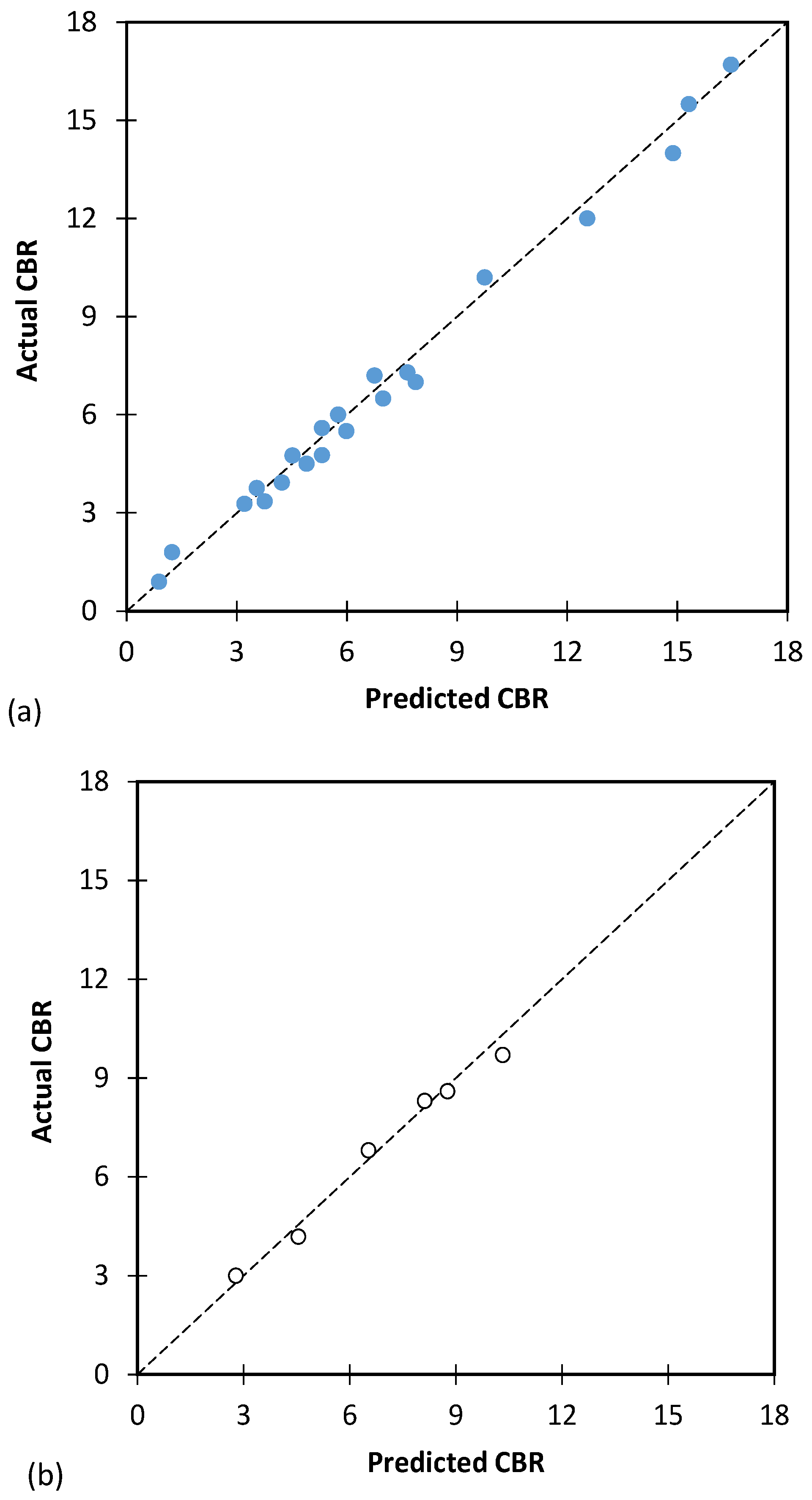
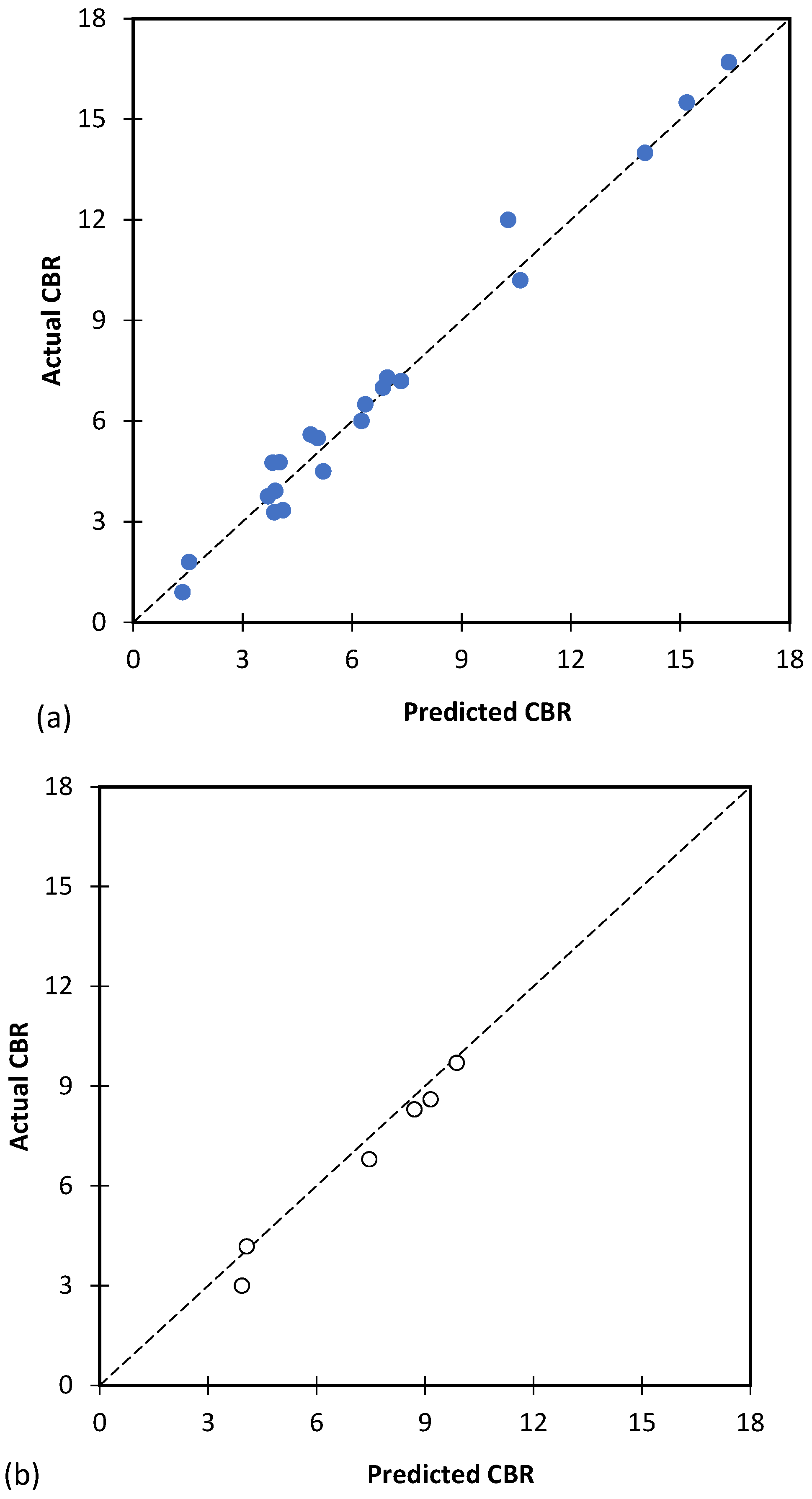
The predicted values of CBR against the values obtained from the test in the laboratory for the training and testing database are shown in
Figure 7. The results show that the SVM model has been able to predict CBR values with good accuracy.
Table 5 presents the performance metrics of an SVM used to predict California Bearing Ratio (CBR) values for a mixture of Alum sludge and soil. Both training and testing data sets were used to evaluate the performance of the SVM model.
The first performance metric is Mean Absolute Error (MAE), which measures the average absolute difference between the predicted and actual CBR values. In both the training and testing sets, the values are 0.497 and 0.512, respectively, indicating that the model has an average error of approximately 0.5. A second performance metric is the Mean Squared Error (MSE), which measures the average squared difference between the predicted and actual CBR values. Both the training and testing sets have values of 0.409 and 0.357, respectively, indicating that the model has a relatively low overall error in predicting CBR values. The third performance metric is the Root Mean Squared Error (RMSE), which is the square root of the Mean Square Error (MSE). Both the training and testing sets have 0.640 and 0.598 values, respectively, indicating that the model has a relatively low overall error in predicting CBR values. In addition to Mean Squared Log Error, the fourth performance metric is Mean Squared Log Error (MSLE). MSLE measures the difference between the logarithm of the predicted CBR values and the logarithm of the actual CBR values. For both the training and testing sets, the values are 0.017 and 0.011, respectively, indicating that the model has a relatively low overall error when predicting CBR values. The fifth performance metric is the Root Mean Squared Log Error (RMSLE), which is the square root of the MSLE. In both the training and testing sets, the values are 0.129 and 0.103 respectively, which indicates that the model has a relatively low overall error in predicting CBR values on a logarithmic scale. The final performance metric is the R2, which measures the amount of variance in the CBR values that can be explained by the model. As can be seen from the values for the training and testing sets, the model has a high degree of correlation between the predicted and actual CBR values. The results suggest that the SVM model is capable of predicting CBR values for the mixture of Alum sludge and soil, as indicated by the low error values and high R-squared values for both training and testing.
4.2. Artificial Neural Network (ANN)
In this study, all artificial neural network (ANN) modeling was performed using MATLAB (R2020a: The Math Works Inc., Natick, MA, USA).
Table 6 displays the results of the Bayesian regularization (BR) and Levenberg-Marquardt (LM) algorithms for all networks. The table contains the
R2 and mean absolute error (MAE) values for both test and training datasets. The results are based on the best-performing network among all 45 neurons and three training repetitions, as determined by the highest
R2 and lowest MAE values.
The findings indicate that the network with two hidden layers achieved the highest performance for both the BR and LM algorithms. Moreover, the average accuracy of the BR algorithm was superior to that of the LM algorithm.
Figure 8 depicts the comparison between the predicted values of the artificial neural network (ANN) model and the actual values of laboratory experiments. The results indicate that the ANN model has exhibited a very high level of precision in predicting the California Bearing Ratio (CBR) values for both the training and testing databases.
Table 7 displays the best outcomes of utilizing the ANN modeling method to predict the California Bearing Ratio (CBR) for the mixtures of alum sludge and soil. The performance indicators of the ANN model are exhibited for both the training and testing datasets. The ANN model yielded a Mean Absolute Error (MAE) of 0.392 and 0.303 for the training and testing datasets, respectively. Similarly, the Mean Squared Error (MSE) values for the training and testing datasets were 0.200 and 0.116, correspondingly. Furthermore, the Root Mean Squared Error (RMSE) values obtained for the training and testing datasets were 0.447 and 0.341, respectively. The ANN model’s Mean Squared Log Error (MSLE) values were 0.005 and 0.002 for the training and testing datasets, respectively, while the Root Mean Squared Log Error (RMSLE) values were 0.074 and 0.046 for the training and testing datasets, respectively. The ANN model yielded a high coefficient of determination (
R²) of 0.989 and 0.980 for the training and testing datasets, respectively, implying that the model is highly precise in predicting the CBR values for a mixture of alum sludge and soil.
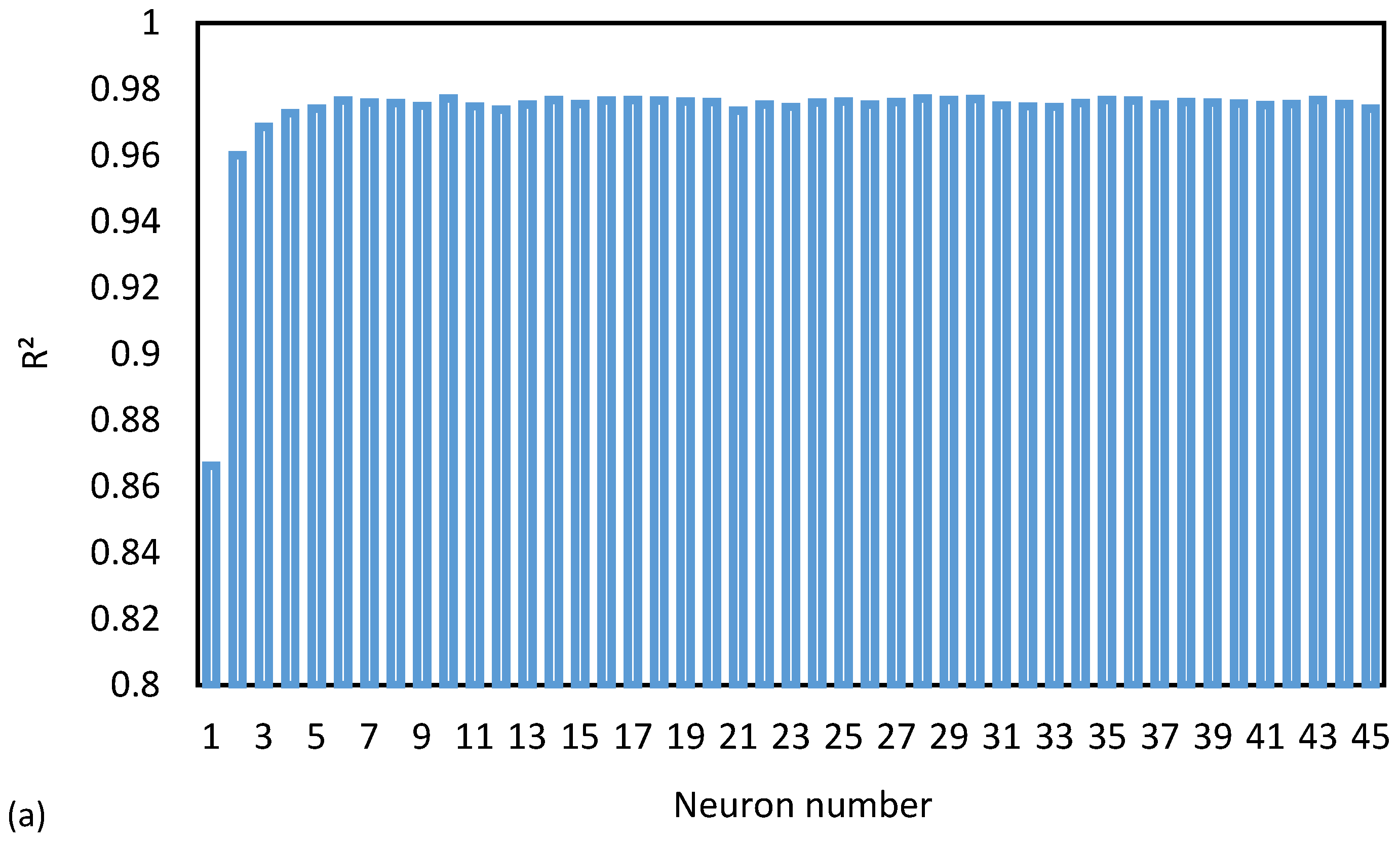
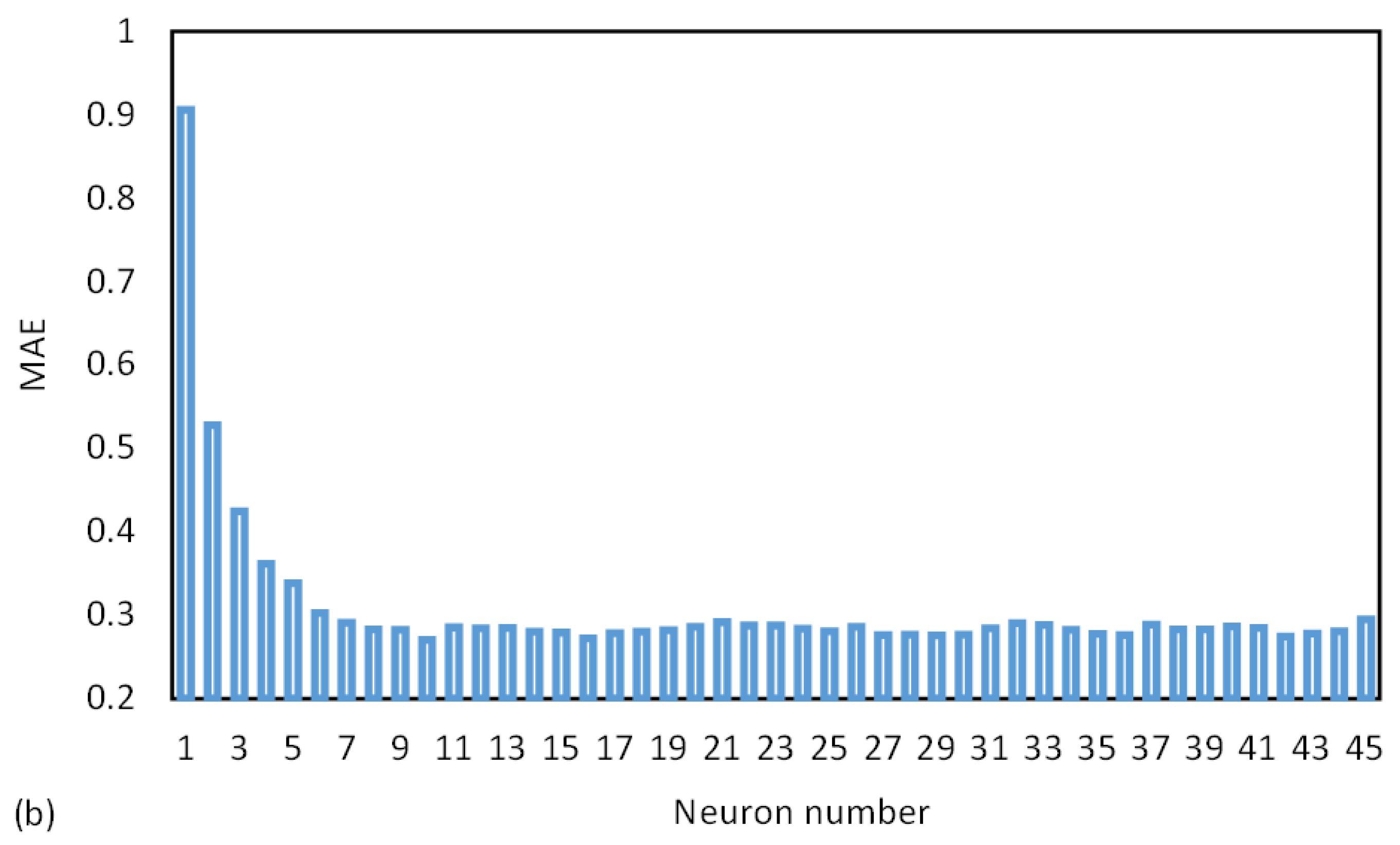
One of the key determinants of the precision and complexity of an artificial intelligence (AI) model is the number of neurons present in each hidden layer. To find the most optimal number of neurons, the group of analyses is conducted.
Figure 9a shows the accuracy of the ANN model based on the number of neurons present in each hidden layer. According to the results, the accuracy of the ANN model does not improve significantly beyond a certain number of neurons which is 10 neurons. Therefore, it is essential to determine the optimal number of neurons to achieve the best accuracy while minimizing the complexity of the model.
Figure 9b displays the model’s error rate for each neuron. The results show that the error rate remains almost constant after the 10th neuron. Thus, the optimal number of neurons for the ANN model was determined to be 10. This information is crucial for researchers and developers of AI models, as it allows them to minimize complexity while achieving the best accuracy. By optimizing the number of neurons, the performance of the AI model can be significantly enhanced.
4.3. Genetic Programming (GP)
The genetics of programming involves applying evolutionary algorithms to generate computer programs through the use of genetic operators such as crossover and mutation. Important parameters that affect the effectiveness of genetic programming include population size, mutation rate, and fitness evaluation function. In this study, after a series of analyses, the best and most optimized GP model was selected based on its ability to produce high-quality programs for a given problem domain.
Figure 10 shows the projected values of CBR by the best GP model against the actual values obtained in the experiments for both training and testing. According to the findings presented in
Figure 10, the best genetic programming (GP) model was capable of accurately predicting the values of California Bearing Ratio (CBR) in the experiments, as indicated by the close match between the model’s projected values and the actual values obtained. These results suggest that the GP model has a high level of accuracy in predicting CBR values.
A significant distinction between genetic programming (GP) and black box models is that the GP produces an equation as an outcome, which can be directly utilized by the reader. In this study, Equation 13 represents the GP model outcome for predicting California Bearing Ratio (CBR) values. The reason for the length of this equation is that it incorporates seven distinct inputs, namely liquid limit, plasticity index, alum sludge content, number of compaction blows, optimum moisture content of soil and mixture, and
Gs of soil. It is worth noting that traditional methods are incapable of producing an equation such as Equation 13, with the consideration of all seven influential inputs. Consequently, this study represents the first successful attempt to formulate an equation for predicting CBR numbers based on these seven important inputs. Also, it is important to notice that the parameters in Equation 1 are normalized value and the readers should normalize their values based on the
Table 1 and then use them in Equation 13.
where
X1,
X2,
X3,
X4 ,
X5 ,
X6 ,
X7 are LL, PI, AS content, number of compaction blows, OMC of soil, OMC of mixture and G
s of soil.
Table 9 presents the results of GP model to predict California Bearing Ratio (CBR) for the mixtures of Alum sludge and soil. The GP model’s performance was evaluated using various performance metrics on both the training and testing datasets. The mean absolute error (MAE) of the model on the training database was 0.459, indicating that, on average, the model’s predictions were off by 0.459 CBR units. The MAE on the testing database was slightly higher at 0.475, indicating that the GP model’s generalization ability was slightly worse than its performance on the training database. The mean squared error (MSE) on the training database was 0.358, indicating that the GP model’s predictions had a higher variance than its performance on the testing database (0.304). The root mean squared error (RMSE) on the training database was 0.598, indicating that the GP model’s predictions had a higher magnitude of error than its performance on the testing database (0.552). The mean squared logarithmic error (MSLE) on the training set was 0.010, and the corresponding value on the testing set was slightly lower at 0.009, indicating that the GP model’s predictions were more accurate on the testing set. The root mean squared logarithmic error (RMSLE) on the training set was 0.100, and the corresponding value on the testing set was slightly lower at 0.097. Finally, the coefficient of determination (
R²) was high for both the training set (0.980) and the testing set (0.948), indicating that the model explained most of the variance in the data and that it had a good fit to the data. In conclusion, the results suggest that the GP model can be used to accurately predict CBR for a mixture of Alum sludge and soil, and that it generalizes well to unseen data. However, the model’s predictions on the training set had a higher variance and magnitude of error compared to the testing set.
5. Discussion
5.1. Comparison of Different Models
Table 10 compares the results of three artificial intelligence (AI) models, namely artificial neural network (ANN), support vector machine (SVM), and genetic programming (GP), to predict the California bearing ratio (CBR) using different performance metrics for both the training and testing databases. The performance metrics used to evaluate the models’ performance include mean absolute error (MAE), mean squared error (MSE), root mean squared error (RMSE), mean squared logarithmic error (MSLE), root mean squared logarithmic error (RMSLE), and coefficient of determination (
R²).
Also,
Table 11 shows the ranking of different AI models. The SVM model was the first AI model examined in this study and is known as a black box model. The ANN method, another black box model, is subsequently employed to explore other black box models’ performance. The GP method is utilized to examine the grey box AI methods.
The results demonstrate that the SVM model exhibits the lowest accuracy for both the training and test datasets, but still, it is a good performance. In contrast, the ANN method performs significantly better and predicts CBR values with high accuracy, achieving R2 of 0.989 and 0.980 for the training and test databases, respectively. The GP method, a grey box model, achieves slightly lower accuracy than the ANN method but still performs well, with R2 of 0.98 and 0.948 for the training and testing databases, respectively. Notably, the GP method offers the benefit of producing an equation as output, which can be used for other datasets.
The reason is that SVM and GP models are known to be better suited for problems with a small number of inputs and a large number of data points, whereas ANN models are better suited for problems with a large number of inputs and a small number of data points. These findings contribute to a better understanding of the performance of different AI models for predicting CBR, which may have implications for future research and practical applications in the field of civil engineering and transportation planning.
5.1 The Variable Importance of Input Parameters
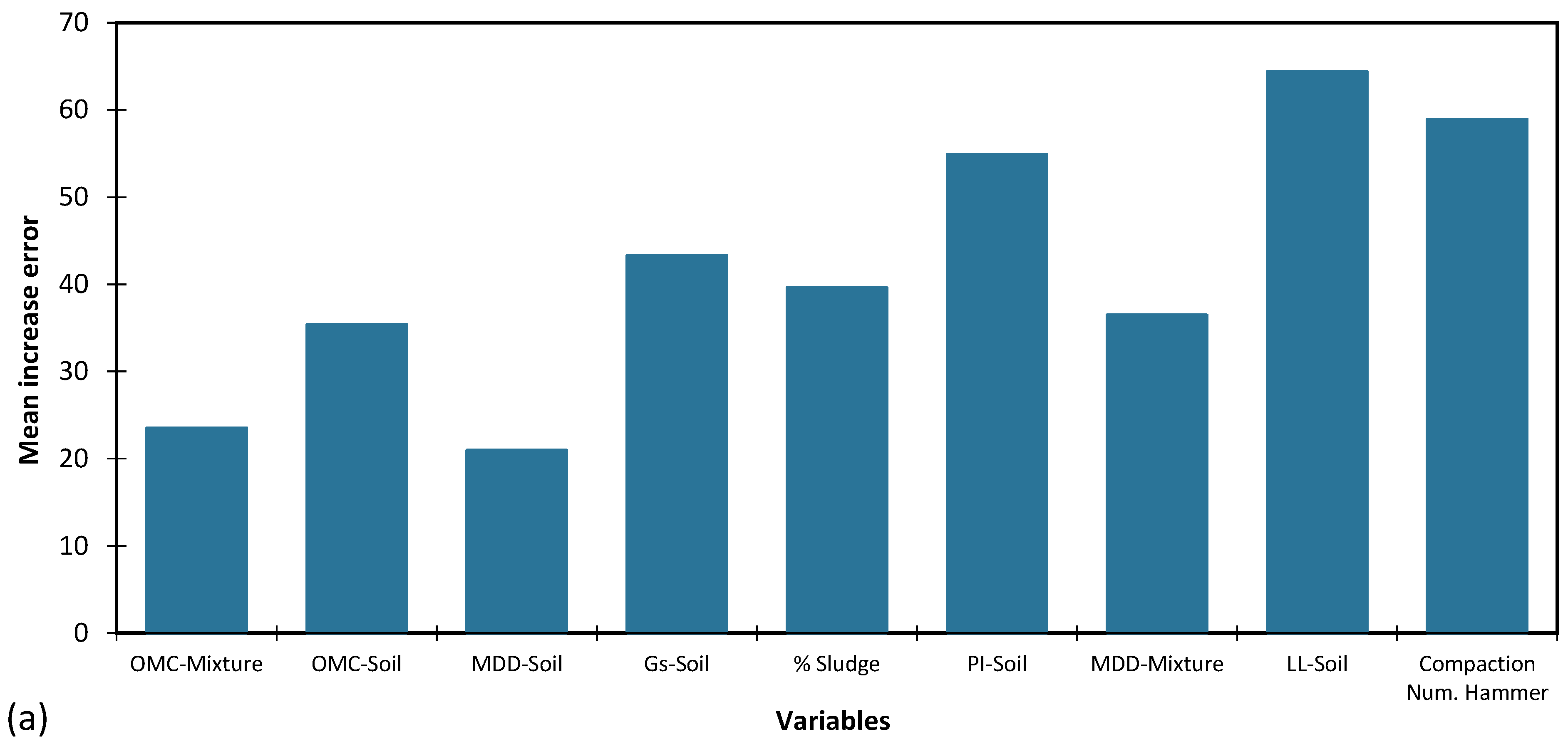
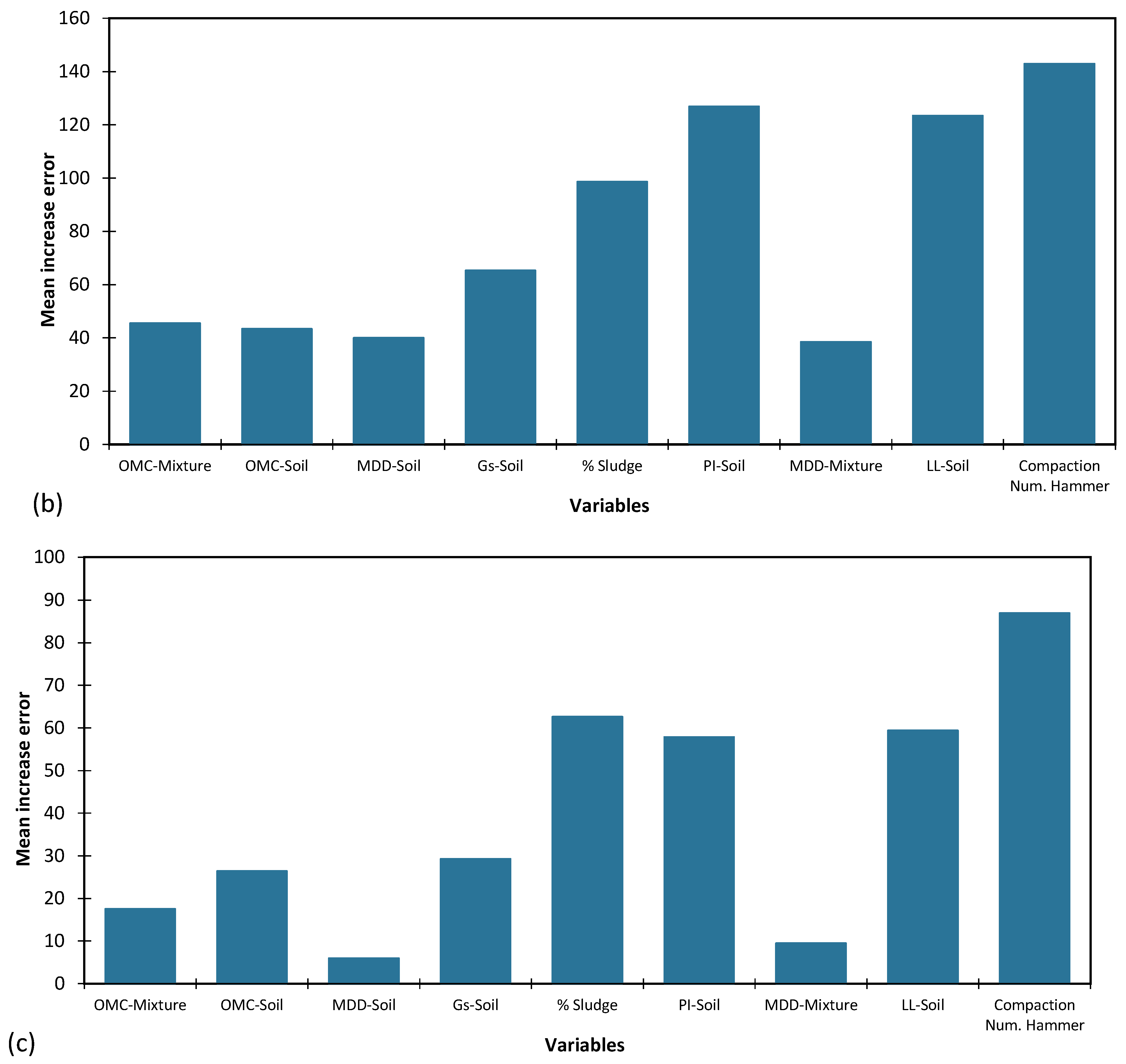
Investigating the significance of input parameters is a crucial aspect of artificial intelligence modelling. In this study, the impact of individual input parameters on network error was examined by altering each parameter by 100%, while maintaining all other inputs at actual values. The resulting network errors were recorded for each alteration and are presented in
Figure 11 for each of the three AI models tested, namely Artificial Neural Networks (ANN), Support Vector Machines (SVM), and Genetic Programming (GP). Greater network error resulting from a given parameter alteration indicates that the network exhibits increased sensitivity to that particular parameter. The variable importance ranking was evaluated based on the input parameters, including Liquid limit of soil (LL-Soil), Plasticity index of soil (PI-Soil),
Gs of soil, number of compaction blows (Compaction Num. Hammer), optimum moisture content of soil (OMC-Soil), maximum dry density of soil (OMC-Mixture), Optimum moisture content of mixture (OMC-mixture), maximum dry density of mixture (MDD-Mixture), and sludge content (% Sludge).
Table 12 summarizes the ranking of inputs based on the different AI models.
The results reveal that the SVM model ranked LL of soil as the most important input parameter, followed by number of compactions blows and PI of soil. While MDD of soil was the least important parameter. Also, ANN ranked number of compactions blows as the most important input parameter, followed by PI and LL of soil. While MDD of mixture was the least important parameter. GP ranked number of compactions blows as the most important input parameter, followed by sludge content and LL of soil. For all three models, and according to
Table 12, it can be concluded that parameters number of compactions blows, and LL of soil are respectively the most important input parameters, while MDD of soil and mixture are the least important.
The explanation for the variation in the importance ranking of input parameters across AI models could be the differences in the underlying algorithms and architectures. SVM is a kernel-based method that tries to find a hyperplane that maximally separates data points. ANN is a feed-forward neural network with hidden layers, and it is trained using a back-propagation algorithm. GP is an evolutionary algorithm that evolves a population of candidate solutions using genetic operators such as mutation and crossover. Therefore, these algorithms have different ways of handling input parameters and constructing models.
Another explanation for the variation in importance ranking could be the nature of the input parameters themselves. Some parameters may have stronger correlations with the target variable, which is CBR, in certain data sets or applications, while others may be less relevant. Moreover, different input parameters may interact with each other in complex ways, making it challenging to determine their individual contributions to the model’s performance.
The California Bearing Ratio (CBR) is a measure of the soil’s load-bearing capacity and is widely used in geotechnical engineering to assess the suitability of soils for construction. The CBR test involves measuring the resistance of a soil sample to penetration by a standard plunger under controlled conditions of moisture and compaction. The stiffness and load-bearing capacity of a soil depend on various factors, including its texture, structure, moisture content, density, and compaction effort. The liquid limit of soil is an important input parameter for predicting CBR because it reflects the soil’s ability to resist deformation and support loads. A soil with a high liquid limit is more plastic and less stable, which results in lower CBR values. In contrast, a soil with a low liquid limit is more rigid and stable, leading to higher CBR values. The number of compaction blows is another critical input parameter for predicting CBR because it represents the compaction effort applied to the soil during construction. The more compaction blows applied, the higher the soil density and stiffness, which result in higher CBR values. Conversely, inadequate compaction effort leads to low soil density and stiffness, resulting in lower CBR values.
Regarding the maximum dry density, it is an indicator of the soil’s compactability and weight. However, it does not directly relate to the soil’s stiffness and load-bearing capacity, which are the primary factors affecting CBR. Therefore, while it may affect CBR values to some extent, its influence is relatively weak compared to other parameters such as liquid limit and compaction effort.
6. Conclusions
The use of Alum sludge in geotechnical engineering has gained importance due to its cost-effectiveness and environmental benefits, as it has been found to improve the strength and stability of soils. CBR test is a crucial parameter in geotechnical engineering, which measures the load-bearing capacity of soil. However, predicting the CBR of soil-Alum sludge mixture can be challenging due to the large number of input variables. This highlights the significance of utilizing artificial intelligence (AI) methods to overcome this challenge, as this approach has not been widely used in this field.
This study aimed to address gaps in the literature by utilizing three different methods, including two black-box models (artificial neural network and support vector machine) and one grey-box model (genetic programming), to predict CBR of soil-Alum sludge mixture. The study compared the performance of the different models using a database of 27 CBR test results on various CBR of soil-Alum sludge mixtures and evaluated the sensitivity and importance of the input parameters. The database consisted of nine parameters, including liquid limit of soil, plasticity index of soil, specific gravity of soil, number of compaction blows, optimum moisture content of soil, maximum dry density of soil, optimum moisture content of mixture, maximum dry density of mixture, and sludge content.
The results show that the SVM model had the lowest accuracy, while the ANN model performed significantly better, achieving high accuracy with R2 of 0.989 and 0.980 for the training and test databases, respectively. The GP method had slightly lower accuracy than the ANN method but still performed well, with R2 of 0.98 and 0.948 for the training and testing databases, respectively. The GP method has the advantage of producing an equation as output, which can be used for other datasets. Overall, the study provides valuable insights into the performance of different AI models for predicting CBR and can be useful for future research and practical applications.
The paper also showed the importance of determining the optimal number of neurons to achieve the best accuracy while minimizing the complexity of the model. The results demonstrated that the accuracy of the ANN model did not improve significantly beyond 10 neurons, indicating that this is the optimal number of neurons. This information is crucial for researchers and developers of AI models, as it allows them to minimize complexity while achieving the best accuracy.
The examination of parameter sensitivity and importance indicated that the number of compaction hammer blows and the soil’s liquid limit were the most significant parameters, while the maximum dry density parameters for soil and mixture were the least significant. This can be attributed to the fact that liquid limit and the number of compaction blows are crucial input parameters for CBR prediction, as they represent the soil’s ability to withstand deformation and support loads. On the other hand, maximum dry density serves as an indicator of soil compactability and weight but has a weaker impact on CBR compared to liquid limit and compaction effort. This information is important for engineers and researchers to optimize their soil stabilization process.
Conflicts of Interest
The authors declare that they have no known competing financial interests or personal relationships that could have appeared to influence the work reported in this paper.
References
- Nguyen, M.D.; Adhikari, S.; Mallya, D.S.; Thomas, M.; Surapaneni, A.; Moon, E.M.; Milne, N.A. Reuse of aluminium-based water treatment sludge for phosphorus adsorption: Evaluating the factors affecting and correlation between adsorption and sludge properties. Environmental Technology & Innovation 2022, 27, 102717. [Google Scholar]
- Nguyen, M.D.; Thomas, M.; Surapaneni, A.; Moon, E.M.; Milne, N.A. Beneficial reuse of water treatment sludge in the context of circular economy. Environmental Technology & Innovation 2022, 102651. [Google Scholar]
- Fiore, F.A.; Rodgher, S.; Ito, C.Y.K. dos Santos Bardini, V.S. and Klinsky, L.M.G., Water sludge reuse as a geotechnical component in road construction: Experimental study. Cleaner Engineering and Technology 2022, 9, 100512. [Google Scholar] [CrossRef]
- Nguyen, M.D.; Baghbani, A.; Alnedawi, A.; Ullah, S.; Kafle, B.; Thomas, M.; Moon, E.M.; Milne, N.A. Experimental Study on the Suitability of Aluminium-Based Water Treatment Sludge as a Next Generation Sustainable Soil Replacement for Road Construction 2023, Available at SSRN 4331275.
- Shaygan, M.; Usher, B.; Baumgartl, T. Modelling Hydrological Performance of a Bauxite Residue Profile for Deposition Management of a Storage Facility. Water 2020, 12, 1988. [Google Scholar] [CrossRef]
- James, J.; Pandian, P.K. Industrial wastes as auxiliary additives to cement/lime stabilization of soils. Advances in Civil Engineering 2016, 624. [Google Scholar] [CrossRef]
- Gonzalez, J.; Sargent, P.; Ennis, C. Sewage treatment sludge biochar activated blast furnace slag as a low carbon binder for soft soil stabilisation. Journal of Cleaner Production 2021, 311, 127553. [Google Scholar] [CrossRef]
- Sahebzadeh, S.; Heidari, A.; Kamelnia, H.; Baghbani, A. Sustainability features of Iran’s vernacular architecture: A comparative study between the architecture of hot–arid and hot–arid–windy regions. Sustainability 2017, 9, 749. [Google Scholar] [CrossRef]
- Odimegwu, T.C.; Zakaria, I.; Abood, M.M.; Nketsiah, C.B.K.; Ahmad, M. Review on different beneficial ways of applying alum sludge in a sustainable disposal manner. Civ. Eng. J 2018, 4, 2230–2241. [Google Scholar] [CrossRef]
- Mohamad, N.; Muthusamy, K.; Embong, R.; Kusbiantoro, A.; Hashim, M.H. Environmental impact of cement production and Solutions: A review. Materials Today Proceedings 2022, 48, 741–746. [Google Scholar] [CrossRef]
- Jiu-Yu, L.I.; Ning, W.A.N.G.; Ren-Kou, X.U.; Tiwari, D. Potential of industrial byproducts in ameliorating acidity and aluminum toxicity of soils under tea plantation. Pedosphere 2010, 20, 645–654. [Google Scholar]
- Shetty, R.; Vidya, C.S.N.; Prakash, N.B.; Lux, A.; Vaculik, M. Aluminum toxicity in plants and its possible mitigation in acid soils by biochar: A review. Science of the Total Environment 2021, 765, 142744. [Google Scholar] [CrossRef] [PubMed]
- Luo, H.L.; Hsiao, D.H.; Lin, D.F.; Lin, C.K. Cohesive soil stabilized using sewage sludge ash/cement and nano aluminum oxide. International Journal of Transportation Science and Technology 2012, 1, 83–99. [Google Scholar] [CrossRef]
- Baghbani, A.; Baumgartl, T.; Filipovic, V. Effects of Wetting and Drying Cycles on Strength of Latrobe Valley Brown Coal (No. EGU23-4804) 2023, Copernicus Meetings.
- Batley, G.E.; Kirby, J.K.; McLaughlin, M.J. Fate and risks of nanomaterials in aquatic and terrestrial environments. Accounts of chemical research 2013, 46, 854–862. [Google Scholar] [CrossRef] [PubMed]
- Huang, J.; Kogbara, R.B.; Hariharan, N.; Masad, E.A.; Little, D.N. A state-of-the-art review of polymers used in soil stabilization. Construction and Building Materials 2021, 305, 124685. [Google Scholar] [CrossRef]
- Jadhav, P.; Sakpal, S.; Khedekar, H.; Pawar, P.; Malipatil, M. Experimental Investigation of Soil Stabilization by Using Aluminium-based sludge.
- Omar, M.B.H.C.; Che Mamat, R.; Abdul Rasam, A.R.; Ramli, A.; Samad, A. Artificial intelligence application for predicting slope stability on soft ground: A comparative study. Int. J. Adv. Technol. Eng. Explor 2021, 8, 362–370. [Google Scholar] [CrossRef]
- Suman, S.; Khan, S.Z.; Das, S.K.; Chand, S.K. Slope stability analysis using artificial intelligence techniques. Natural Hazards 2016, 84, 727–748. [Google Scholar] [CrossRef]
- Baghbani, A.; Daghistani, F.; Naga, H.A.; Costa, S. Development of a Support Vector Machine (SVM) and a Classification and Regression Tree (CART) to Predict the Shear Strength of Sand Rubber Mixtures. In Proceedings of the 8th International Symposium on Geotechnical Safety and Risk (ISGSR), Newcastle, Australia 2022. [Google Scholar]
- Lin, S.S.; Shen, S.L.; Zhang, N.; Zhou, A. Modelling the performance of EPB shield tunnelling using machine and deep learning algorithms. Geoscience Frontiers 2021, 12, 101177. [Google Scholar] [CrossRef]
- Baghbani, A.; Baghbani, H.; Shalchiyan, M.M.; Kiany, K. Utilizing artificial intelligence and finite element method to simulate the effects of new tunnels on existing tunnel deformation. Journal of Computational and Cognitive Engineering 2022. [CrossRef]
- Ayawah, P.E.; Sebbeh-Newton, S.; Azure, J.W.; Kaba, A.G.; Anani, A.; Bansah, S.; Zabidi, H. A review and case study of Artificial intelligence and Machine learning methods used for ground condition prediction ahead of tunnel boring Machines. Tunnelling and Underground Space Technology 2023, 125, 104497. [Google Scholar] [CrossRef]
- Tijanić, K.; Car-Pušić, D.; Šperac, M. Cost estimation in road construction using artificial neural network. Neural Computing and Applications 2020, 32, 9343–9355. [Google Scholar] [CrossRef]
- Anysz, H.; Foremny, A.; Kulejewski, J. February. Comparison of ANN classifier to the neuro-fuzzy system for collusion detection in the tender procedures of road construction sector. In IOP Conference Series: Materials Science and Engineering 2019, Vol. 471, p 112064. IOP Publishing.
- Xu, J.J.; Zhang, H.; Tang, C.S.; Cheng, Q.; Tian, B.G.; Liu, B.; Shi, B. Automatic soil crack recognition under uneven illumination condition with the application of artificial intelligence. Engineering Geology 2022, 296, 106495. [Google Scholar] [CrossRef]
- Baghbani, A.; Costa, S.; Choundhury, T.; Faradonbeh, R.S. Prediction of Parallel Desiccation Cracks of Clays Using a Classification and Regression Tree (CART) Technique. In Proceedings of the 8th International Symposium on Geotechnical Safety and Risk (ISGSR), Newcastle, Australia 2022. [Google Scholar]
- Onyelowe, K.C.; Aneke, F.I.; Onyia, M.E.; Ebid, A.M.; Usungedo, T. AI (ANN, GP, and EPR)-based predictive models of bulk density, linear-volumetric shrinkage & desiccation cracking of HSDA-treated black cotton soil for sustainable subgrade. Geomechanics and Geoengineering 2022, 1–20. [Google Scholar]
- Lawal, A.I.; Kwon, S. Application of artificial intelligence to rock mechanics: An overview. Journal of Rock Mechanics and Geotechnical Engineering 2021, 13, 248–266. [Google Scholar] [CrossRef]
- Tariq, Z.; Elkatatny, S.M.; Mahmoud, M.A.; Abdulraheem, A.; Abdelwahab, A.Z.; Woldeamanuel, M. Estimation of rock mechanical parameters using artificial intelligence tools. In 51st US Rock Mechanics/Geomechanics Symposium. OnePetro 2017. [Google Scholar]
- Njock, P.G.A.; Shen, S.L.; Zhou, A.; Lyu, H.M. Evaluation of soil liquefaction using AI technology incorporating a coupled ENN/t-SNE model. Soil Dynamics and Earthquake Engineering 2020, 130, 105988. [Google Scholar] [CrossRef]
- Baghbani, A.; Choudhury, T.; Samui, P.; Costa, S. Prediction of secant shear modulus and damping ratio for an extremely dilative silica sand based on machine learning techniques. Soil Dynamics and Earthquake Engineering 2023, 165, 107708. [Google Scholar] [CrossRef]
- Baghbani, A.; Costa, S.; O’Kelly, B.C.; Soltani, A.; Barzegar, M. Experimental study on cyclic simple shear behaviour of predominantly dilative silica sand. International Journal of Geotechnical Engineering 2022, 1–15. [Google Scholar] [CrossRef]
- Baghbani, A.; Costa, S.; Faradonbeh, R.S.; Soltani, A.; Baghbani, H. Experimental-AI Investigation of the Effect of Particle Shape on the Damping Ratio of Dry Sand under Simple Shear Test Loading 2023, preprint.
- Baghbani, A.; Daghistani, F.; Baghbani, H.; Kiany, K. Predicting the Strength of Recycled Glass Powder-Based Geopolymers for Improving Mechanical Behavior of Clay Soils Using Artificial Intelligence (No. 9741). EasyChair 2023.
- Baghbani, A.; Daghistani, F.; Baghbani, H.; Kiany, K. Predicting the Strength of Recycled Glass Powder-Based Geopolymers for Improving Mechanical Behavior of Clay Soils Using Artificial Intelligence (No. 9741). EasyChair 2023.
- Baghbani, A.; Daghistani, F.; Kiany, K.; Shalchiyan, M.M. AI-Based Prediction of Strength and Tensile Properties of Expansive Soil Stabilized with Recycled Ash and Natural Fibers (No. 9743). EasyChair 2023.
- Baghbani, A.; Choudhury, T.; Costa, S.; Reiner, J. Application of artificial intelligence in geotechnical engineering: A state-of-the-art review. Earth-Science Reviews 2022, 228, 103991. [Google Scholar] [CrossRef]
- Aamir, M.; Mahmood, Z.; Nisar, A.; Farid, A.; Ahmed Khan, T.; Abbas, M.; Ismaeel, M.; Shah, S.A.R.; Waseem, M. Performance evaluation of sustainable soil stabilization process using waste materials. Processes 2019, 7, 378. [Google Scholar] [CrossRef]
- Shah, S.A.R.; Mahmood, Z.; Nisar, A.; Aamir, M.; Farid, A.; Waseem, M. Compaction performance analysis of alum sludge waste modified soil. Construction and Building Materials 2020, 230, 116953. [Google Scholar] [CrossRef]
- Giustolisi, O.; Doglioni, A.; Savic, D.A.; Webb, B.W. A multi-model approach to analysis of environmental phenomena. Environ Model Softw 2007, 22, 674–682. [Google Scholar] [CrossRef]
- Zhang, Q.; Barri, K.; Jiao, P.; Salehi, H.; Alavi, A.H. Genetic programming in civil engineering: Advent, applications and future trends. Artificial Intelligence Review 2021, 54, 1863–1885. [Google Scholar] [CrossRef]
- Vapnik, V.N. An overview of statistical learning theory. IEEE transactions on neural networks 1999, 10, 988–999. [Google Scholar] [CrossRef] [PubMed]
- Rosenblatt, F. The perceptron: a probabilistic model for information storage and organization in the brain. Psychological review 1958, 65, 386. [Google Scholar] [CrossRef] [PubMed]
- Rumelhart, D.E.; Hinton, G.E.; Williams, R.J. Learning representations by back-propagating errors. nature 1986, 323, 533–536. [Google Scholar] [CrossRef]
- LeCun, Y.; Bengio, Y.; Hinton, G. Deep learning. nature 2015, 521, 436–444. [Google Scholar] [CrossRef] [PubMed]
- Shanmuganathan, S. Artificial neural network modelling: An introduction. Springer International Publishing 2016, 1–14. [Google Scholar]
- Dongare, A.D.; Kharde, R.R.; Kachare, A.D. Introduction to artificial neural network. International Journal of Engineering and Innovative Technology (IJEIT) 2012, 2, 189–194. [Google Scholar]
- Macukow, B. Neural networks–state of art, brief history, basic models and architecture. In Computer Information Systems and Industrial Management: 15th IFIP TC8 International Conference, CISIM 2016, Vilnius, Lithuania, September 14-16 2016, Proceedings 15 (pp. 3-14). Springer International Publishing.
- Sun, Y.; Zeng, W.D.; Zhao, Y.Q.; Qi, Y.L.; Ma, X.; Han, Y.F. Development of constitutive relationship model of Ti600 alloy using artificial neural network. Computational Materials Science 2010, 48, 686–691. [Google Scholar] [CrossRef]
- Agatonovic-Kustrin, S.; Beresford, R. Basic concepts of artificial neural network (ANN) modeling and its application in pharmaceutical research. Journal of pharmaceutical and biomedical analysis 2000, 22, 717–727. [Google Scholar] [CrossRef]
- Marquardt, D.W. An algorithm for least-squares estimation of nonlinear parameters. Journal of the society for Industrial and Applied Mathematics 1963, 11, 431–441. [Google Scholar] [CrossRef]
- Burden, F.; Winkler, D. Bayesian regularization of neural networks. Artificial neural networks: methods and applications 2009, 23–42. [Google Scholar]
|
Disclaimer/Publisher’s Note: The statements, opinions and data contained in all publications are solely those of the individual author(s) and contributor(s) and not of MDPI and/or the editor(s). MDPI and/or the editor(s) disclaim responsibility for any injury to people or property resulting from any ideas, methods, instructions or products referred to in the content. |
© 2023 by the authors. Licensee MDPI, Basel, Switzerland. This article is an open access article distributed under the terms and conditions of the Creative Commons Attribution (CC BY) license (http://creativecommons.org/licenses/by/4.0/).
