1. Introduction
Sandy beaches provide a natural barrier for coastal protection against marine storms. Also, they are a key asset for coastal tourism and socioeconomic system of many countries ( Di Luccio et al., 2018). Particularly, the Mediterranean coastal zone is severely impacted by extreme climatic events (e.g., storm surges and high waves) coupled with human-induced pressures (e.g., uncontrolled coastal urbanization), resulting in a growing vulnerability (Mejjad et al., 2022; Satta et al., 2017). In consequence, assessing how climate change, and in particular, the projected changes of sea level and wind waves can affect the sandy beaches is of paramount importance.
The magnitude of beach flooding depends on the total water level at the coast. In turn, this depends on the astronomical tidal level, changes in the mean sea level, the storm surge and the wave runup (Holman and Guza, 1984). Regarding the later, as waves approach the coast, part of the energy dissipates due to wave-breaking in the surf zone and the remaining energy reaches the beach and drives oscillations of the water edge over the foreshore (Gomes da Silva et al., 2018). The vertical value of this oscillations is called runup, composed of a steady super elevation called setup, and a fluctuating component called swash (Holman and Guza, 1984; Stockdon et al., 2006). In regions with small tidal range and relatively mild storm surges, like the Mediterranean Sea (Amores et al., 2020; Marcos and Tsimplis, 2007; Tsimplis et al., 1995), the wave runup can represent the main contributor of the total water level under extreme wave conditions (Agulles et al., 2021).
In the last decades, great efforts have been done to develop wave runup empirical equations based on field observations (Gomes da Silva et al., 2020). Among them, Stockdon et al. (2006) have developed an empirical formulation that has become a standard in runup computations. Based on the work of Holman, (1986) and gathering the information obtained in ten field experiments, Stockdon et al. (2006; hereinafter S2006) fitted runup observations from video cameras to beach slope and incident wave parameters. They have obtained a formulation for the setup and swash that has been widely used with reliable results in many different contexts (e.g: Atkinson et al., 2017; Di Luccio et al., 2018). A foreseen problem with this formulation is that it does not take into account the modification of wave parameters by refraction, diffraction, bottom friction and breaking, among other effects, that take place when the waves approach the coast. Alternatively, the use of wave phase-resolving numerical models capable to simulate the wave runup in the swash zone has increased in the last years thanks to the increase of computational power (Enríquez et al., 2019; Roelvink et al., 2018; Zijlema et al., 2011). While numerical models offer greater flexibility and are capable of simulating complex coastlines and bathymetries, they entail a much higher computational cost compared to using empirical equations. Additionally, the calibration of numerical models requires suitable data, which can add to the complexity and cost of their implementation. Both approaches, the empirical and the numerical, have been applied to a broad variety of situations. In particular, projections of future beach flooding due to global warming have been implemented using empirical approaches (Didier et al., 2015; Vousdoukas et al., 2020), numerical ones (Agulles et al., 2021; Enríquez et al., 2019; Orejarena-Rondón et al., 2019) or mixed ones (Stockdon et al., 2014).
Uncertainties associated to climate projections are an important information that must be provided to stakeholders (Cobb et al., 2021). Those uncertainties come from several sources like future greenhouse gas emissions (GHG), natural variability or model limitations (Giorgi, 2010; Hawkins and Sutton, 2009; Horton et al., 2020; Oddo et al., 2020). The first two sources are commonly addressed by running ensembles of model simulations under different GHG scenarios (Hawkins and Sutton, 2009). The third one, however, requires from specific studies that consider the particularities of the modelling system, defined hereinafter as the model itself, as well as its particular configuration and the boundary conditions used to force it. In the case of beach flooding some studies have quantified the quality of the model results during short periods of time corresponding to field experiments on a specific beach (Di Luccio et al., 2018; Gomes da Silva et al., 2018; Xie et al., 2019). However, up to our knowledge there has not been a detailed comparison on how different elements of the modelling system impact on the accuracy of the wave runup estimates for an extended period of time.
The goal of this paper is to quantify the errors associated with estimates of wave runup on sandy beaches, and to assess how these errors vary depending on the choices adopted in the modelling setup. The strategy followed has been to implement several modelling approaches based on empirical and numerical models with different degrees of complexity (1D and 2D) and to compare their results with a long time series of observations in two different sandy beaches which are representative of Mediterranean beach typology. This quantification of the error sources can help to assess the relative impact of model limitations in the uncertainties associated to projections of future wave runup.
The work is organized as follows. In
Section 2, data and site description are presented along with the methodology of the experimental protocol proposed to obtain the wave runup uncertainties. Results of the different methodologies proposed are shown in section 3. To conclude, discussion and conclusions are presented in sections 4 and 5.
2. Data and methods
2.1. Study Sites
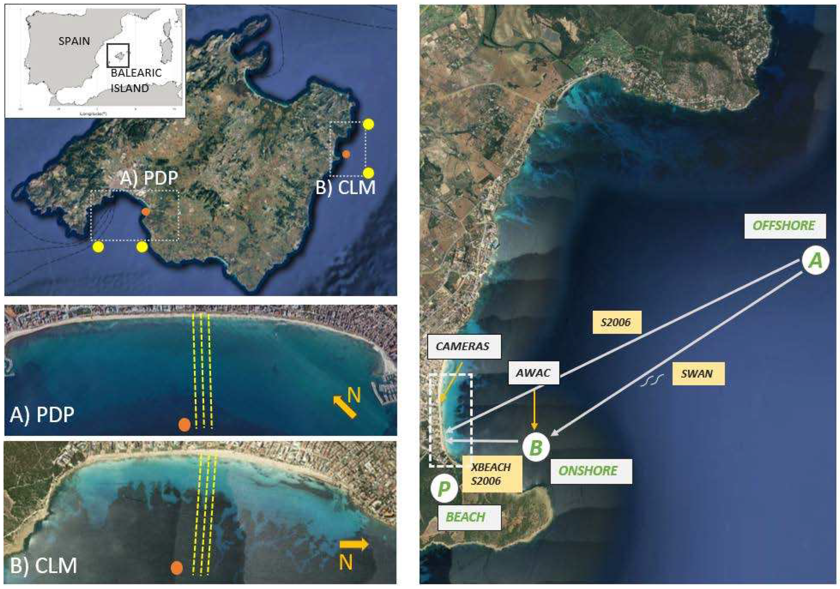
In this work we analyse two microtidal sandy beaches located in the Mallorca Island (Western Mediterranean Sea, see
Figure 1). These beaches can be considered representative of a large fraction of Mediterranean sandy beaches. Specifically, the Playa de Palma beach (hereinafter, PDP) located on the South of the island and Cala Millor beach (hereinafter, CLM) located on the East. PDP is a large beach of ~4.5 km alongshore by ~30-50 m wide with fine grain size (0.20-0.25mm of D50) and relatively low slope of ~0.027 with dissipative conditions (
Figure 1a). CLM is ~1.7 km alongshore by 35-40 m wide, with a mixed rock and sand bed and a small cliff at the southernmost sector of the beach. It has a medium grain size (0.35-0.40mm of D50) with a mean beach slope ~0.044 and slightly reflective conditions (
Figure 1b). The two beaches are included in the beach monitoring programme of the Balearic Islands Coastal Observing and Forecasting System (SOCIB) since 2011. This programme includes periodic topography and bathymetry surveys, continuous video monitoring of the shoreline position and in situ measurements of nearshore waves and currents, among others (Tintoré et al., 2013).
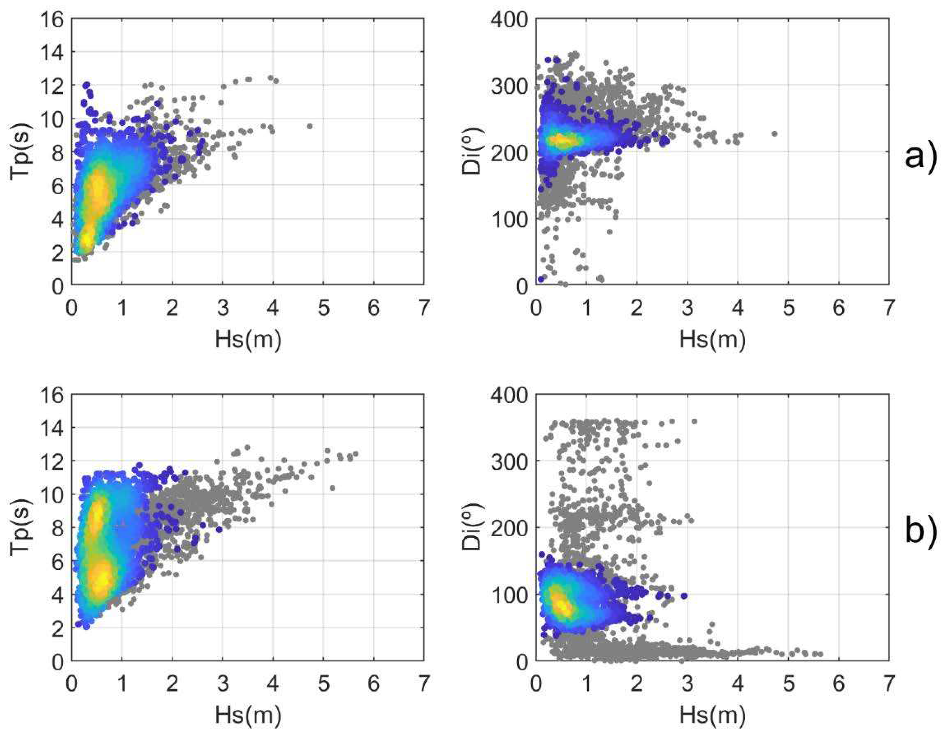
The wave conditions in both sites are showed in
Figure 2. The mean conditions of the two locations are similar with significant wave height (Hs) around 0.5-1.0 m and a peak period (Tp) of around 5-6 s. PDP is exposed to offshore wave conditions from the SSW to SW (dominant direction ~200º) and this dominant direction is kept as the waves refract and approach the shoaling zone (
Figure 2a). In contrast, in CLM there are large differences between offshore and onshore wave conditions, both for the mean and extreme waves (
Figure 2b). The offshore waves arrive from NNE to SSE (directions from ~30º to 150º) while the nearshore mean direction is around E (~100 º) due to diffraction.
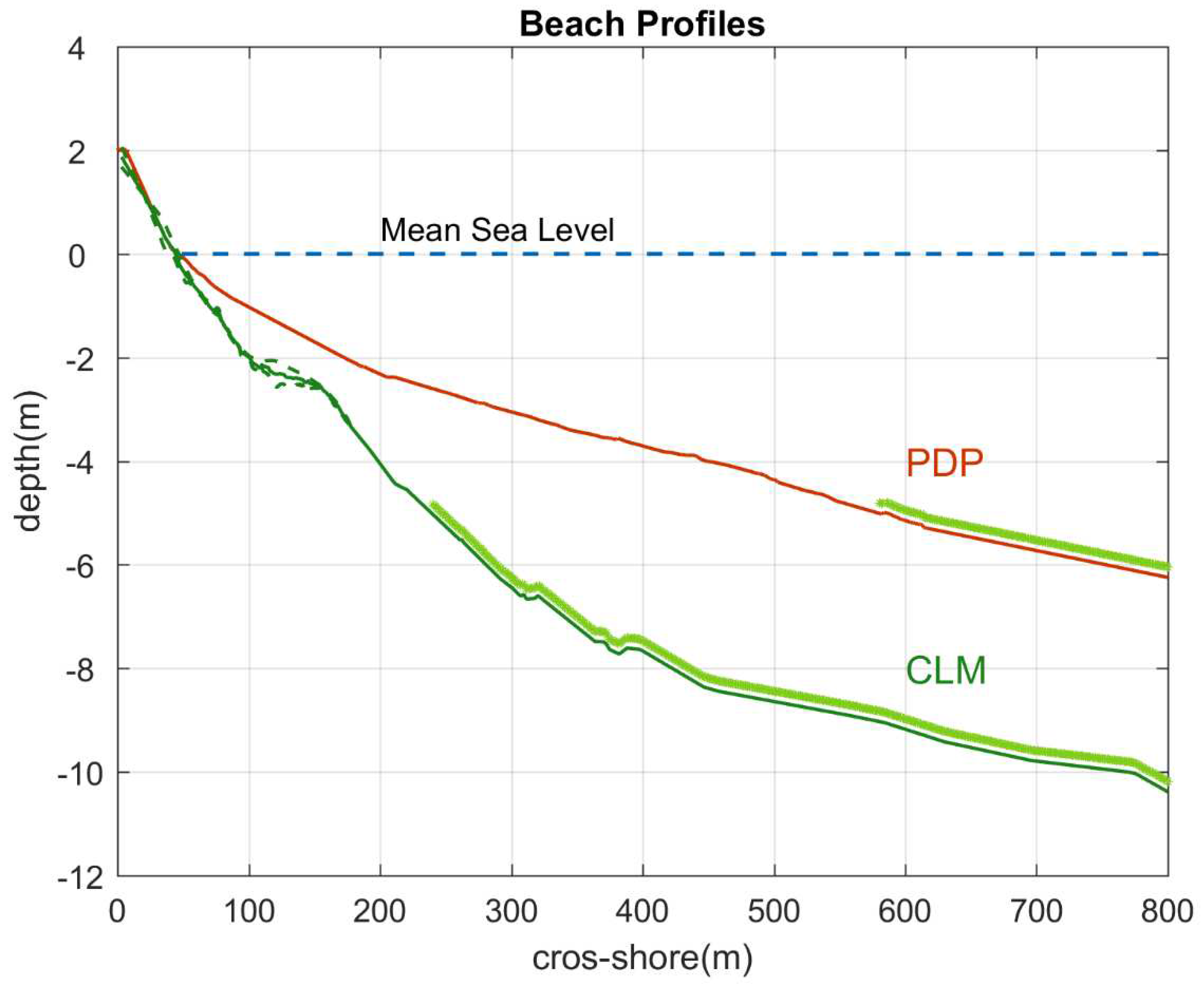
An important characteristic of Mediterranean coasts is the presence of vegetation in seabed. Seagrass meadows are commonly present at shallow depths in the whole basin and therefore along the coast in our study region (Cebrián et al., 1996; Ruiz et al., 2015; Telesca et al., 2015). In particular, the presence of seagrass is constant from depths between 5 and 40 m both in PDP and CLM (
Figure 3). This fact determines the magnitude of the bottom friction and has been carefully considered in the model configuration (see
Section 2.6.2).
2.2. Topo-Bathymetric Surveys
Bathymetry surveys were conducted by SOCIB (Tintoré et al., 2013), using a single-beam echo sounder, BioSonics DT/DE Series Digital Echosounder, in the CLM beach and a multi-beam echo sounder, R2Sonic2020, in PDP. The final spatial resolution is 1 m x 1 m. These measurements were complemented with topographies of the aerial beach obtained using a survey-grade RTK-GPS (Real Time Kinematic Global Position System). The surveys were conducted under calm conditions and more information can be found in
https://medclic.es/en/instrumentos/monitorizacion-de-playas/.
The characteristic cross-shore profile of each beach is obtained by averaging the transects located in the middle of the beach (area limited by yellow dashed lines in
Figure 1a and b). Winter and summer profile are available for CLM while only summer profile is available for PDP (
Figure 3). The beach slope (
) is calculated as the average slope over the swash zone. This zone has been delimited from the observed horizontal swash variability (see video imagery section).
2.3. Wave Data
Nearshore waves observations at hourly resolution are obtained from directional Acoustic Waves and Currents (AWACs) sensors located at ~20 m water depth at the two studied beaches (
Figure 1, orange dots), covering a period from 2012 to 2017 at PDP beach and from 2011 to 2019 at CLM beach. Data have been downloaded from
http://thredds.socib.es/thredds/catalog.html, and the wave parameters for each beach are presented in
Figure 2.
Offshore waves conditions were retrieved from the SIMAR database developed and maintained by Puertos del Estado (Pilar et al., 2008). SIMAR is a 62-year wave reanalysis generated with the WAM model (Hasselmann et al., 1988) from 1958 to 2020. It covers part of the Atlantic ocean and the Western Mediterranean (Longitude -12º to 8º and Latitude 34º to 48º) with a spatial resolution of ~3 Km and hourly temporal resolution (see yellow dots
Figure 1 for locations, and in Fig 2). Data can be obtained throughout the Puertos del Estado dataserver at
https://www.puertos.es/es-es/oceanografia/Paginas/portus.aspx.
2.4. Video Imagery
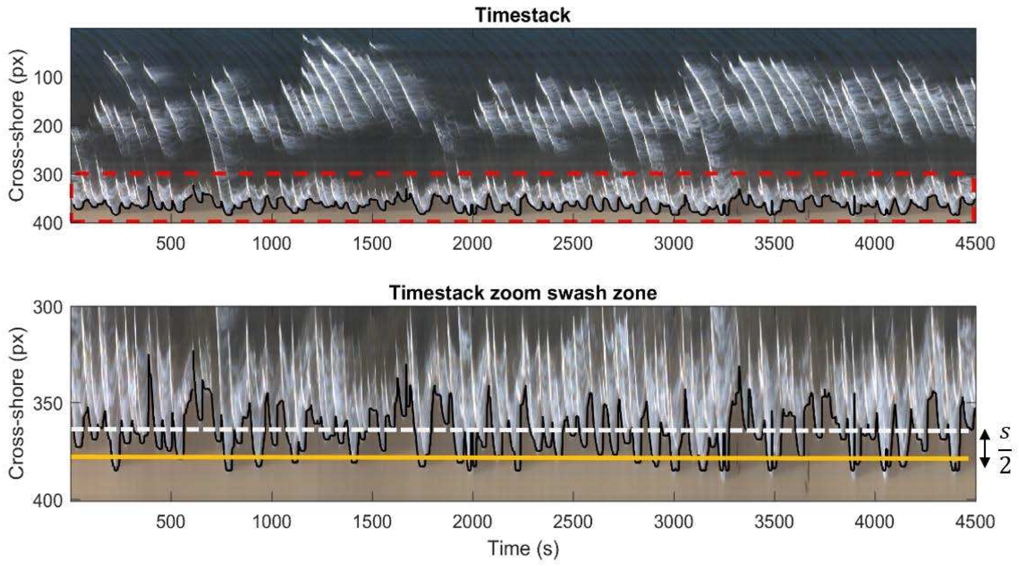
Timestack images cover the period from 2012 to 2017 in PDP and from 2011 to 2018 in CLM. Those images has been provided by the SOCIB beach monitoring facility (Alvarez-ellacuria et al., 2011). Timestack shows a cross-shore transects of pixel intensity sampled at 7.5 Hz over 10 minutes every hour (Simarro et al., 2017). This created timestack of pixel intensity, on which wave runup and rundown are showed as a black edge moving back and forth in the swash zone (
Figure 4). A quality control was applied to keep only those images clear enough to extract information on the wave runup. As a result, 2015 images were kept for PDP and 1909 images for CLM.
The wave runup is composed by a steady super elevation called setup () and a fluctuating component called swash () (Holman and Guza, 1984). In order to extract the setup from images, it would be necessary to know where exactly the coastline in calm conditions is located for each of the timestacks. Unfortunately, this is challenging because the coastline has been modified either by natural causes or by human intervention (e.g., beach nourishment) during the time covered by the images (i.e., 5 years at PDP and almost 8 years at CLM). Consequently, direct observations of wave setup were unavailable to validate the model results. Nevertheless, in order to have an idea about how crucial that could be for the goal of this work, we have compared the relative importance of setup and swash contributions to the total wave runup (see figure SI1). The setup component has been computed using the S2006 formulation and XBEACH simulations fed with nearshore waves from AWACs, while the swash has been infered from the images. The results show that setup is ~25-30% of the wave runup, so eventual unaccuracies in their estimates may be considered of second order of importance with regard to the goal of this study.
Therefore, we have decided to remove the mean value of the runup computed from each timestack, and thus obtaining only observations of the swash. In particular, the swash component is estimated as the 98% quantile of the water/land transition time series (
Figure 4 yellow line, bottom panel) respect to the mean value (
Figure 4 white dashed line, bottom panel). Thereby the swash 2% is retrieved from each timestack. Once the swash observations are obtained, it is necessary to transfer the horizontal swash to the vertical component using the beach slope (,
. Following previous works (Stockdon et al., 2006; Vousdoukas et al., 2012) ,
is defined as the average slope over a region ±2*STD around the swash zone, where STD is the standard deviation of the horizontal swash variability. Thus for PDP
is 0.027 and for CLM is 0.044. The standard deviation of the resulting vertical swash in PDP is 0.06 m and 0.12 m in CLM.
2.5. Empirical Runup Estimates
In this work we use the S2006 formulation as it is one of the most widespread empirical approaches used to estimate wave runup. The expression for
(i.e., the wave runup elevation which is exceeded by 2% of the incident waves) is composed by two terms, the setup (
) and the swash (
):
where
represent the beach slope at the swash zone,
the significant wave height and
the wavelength.
2.6. Numerical Approach
2.6.1. Nearshore Wave Climate
The SWAN numerical model (Booij and Holthuijsen, 1987) is used to propagate the offshore maritime climate up to the coast. SWAN is a third-generation wave model that solves the spectral action balance equation for the propagation of wave spectra (
http://swanmodel.sourceforge.net/). This model allows an accurate and computationally feasible simulation of waves in relatively large areas (Camus et al., 2013; Enríquez et al., 2017; Orejarena-Rondón et al., 2019). SWAN simulations are performed in a stationary mode over a regular 200 x 200 m grid (see gray dashed rectangles in
Figure 1). The boundary conditions to drive the model have been extracted from the closest SIMAR point located in deep waters (
Figure 1, yellow dots). The propagated sea states have been the same than those occurring in the period covered by the observations (Figure SI2 black dots). The model outputs in terms of Hs, Tp and mean direction have been extracted from the simulations at the same depths where AWACs are installed (~20 m depth). A comparison between the modelled nearshore waves and the waves recorded by the AWACs in PDP and CLM is shown in Figure SI3. A high agreement is found between observed and modelled nearshore waves with a root mean square error (RMSE) of 0.24 m and 0.22 m and a correlation of 0.86 and 0.86 for PDP and CLM, respectively.
2.6.2. Wave Runup
The wave propagation until the swash zone and the wave runup on the beach are simulated using the XBEACH model (Roelvink et al., 2015). XBEACH is an open-source numerical model which originally was developed to simulate hydrodynamic and morphodynamic processes and impacts on sandy beaches. The model solves the phase-averaged coupled equations for cross-shore and longshore hydrodynamics and morphodynamics. XBEACH has been implemented and validated in many situations (e.g: Harley et al., 2011; Roelvink et al., 2018; Vousdoukas et al., 2012b) becoming a standard faithfully tool for runup computations provided the model parameters were previously calibrated. The model is forced by observed or simulated nearshore waves (
Figure 1, orange dots) and has been implemented in 1D and 2D modes. The 1D runs were carried out without directonal spreading and assuming the waves to be perpendicular to the coastline orientation, with a cross-shore spatial resolution (dx) of 1 m and 20 minutes of Jonswap espectra mode. The 2D runs were implemented with a spatial resolution of 2 m in the cross-shore direction and 10m in the alongshore direction with the same set up of the 1D simulations.
The most important transformation in the wave characteristics occurs in the shoaling and breaking zones where the energy is considerably reduced. Moreover, in this critical zone, the bottom friction plays a paramount role in the wave dissipation, specially over vegetation grounds (Beck et al., 2018; Duarte et al., 2013; Menéndez et al., 2020). As we pointed out in section 2.1, the seagrass meadows are commonly present at shallow depths along the Mediterranean coasts and therefore in our study region (Cebrián et al., 1996; Ruiz et al., 2015; Telesca et al., 2015). In particular, the presence of seagrass is almost constant from depths between 5 and 40 m both in PDP and CLM (
Figure 3). Consequently, the vegetation module in XBEACH has been activated in the simulations. This module includes wave damping and wave breaking over vegetation fields at variable depths. Based on nonlinear formulation of the drag force, either irregular or monochromatic waves can be modelled considering geometric and physical characteristics of the vegetation field (Mendez and Losada, 2004; van Rooijen et al., 2015). In particular, the vegetation stem diameter (Bv), the mean shoot length (Ah), the vegetation density (N) and the drag coefficient (
) are parameters affecting the wave evolution and are included in the vegetation module. The first three parameters were set to the observed values in the region (Bv= 0.02 m, Ah = 0.35 m and N= 615 shoots/m
2 , de los Santos et al., 2019; Infantes et al., 2012).
In order to calibrate the drag coefficient, wave observations from another field experiment (Infantes et al., 2012) have been used. In that experiment, the wave height was measured along a cross-shore transect in CLM beach during the period from 7 to 23 July 2009 (see Figure SI4). In that beach, seagrass was present up to a depth of 6 m and the nearshore wave height observed during the experiment ranged from 0.3 to 1.2 m when a moderate storm hit the area. The wave propagation during the same period was simulated using XBEACH testing different values for the drag coefficient. The optimal value found was to use CD = 0.05, leading to a good agreement between the modelled and observed cross-shore wave transformation (see Figure SI4).
Simulating with XBEACH all the sea states corresponding to the available timestack observations (3924 cases in total for PDP and CLM) would require a highly computational effort. To overcome this, a clustering technique has been used to select a statistically representative set of sea states following two steps. First, sea states with directions out of ±30º with respect to the cross-shore direction and periods shorter than 4s have been discarded. Then, among the remaining ones, 100 sea states were selected using the k-means algorithm (Figure SI2 green dots). Those 100 states have been simulated to obtain the corresponding wave runup. Finally, the complete time series of wave runup has been reconstructed through the analogues identification method (see Camus et al., (2011) for the details of the methodology).
2.7. Experimental Protocol
In this study we aim at assessing the relative importance of different sources of error in the swash and setup computation. To do so, a series of complementary simulations have been performed with different configurations of the models (
Table 1). First, the calibrated XBEACH model is run in its 2D version and forced with observed bathymetry, seagrass coverage and nearshore waves from the AWAC. This simulation NUM2D-OBS will be considered as the benchmark run. Then, several simplifications of the system are considered. First, XBEACH is run with the same forcing but in its 1D version (NUM1D-OBS run). Next, the empirical formulation is utilized, based on the observed bathymetric slope and forced with nearshore waves, (EMP-OBS run). Then, instead of using observed nearshore waves, the empirical formulation is forced with simulated nearshore waves (EMP-ON run). Finally, the simplest approach is to use the empirical formulation using offshore waves from SIMAR (EMP-OFF run). This is the easiest most common approach since information on open sea waves is usually available from wave hindcasts.
Complementary, a set of sensitivity experiments have been also performed to estimate the impact of uncertainties in the bathymetric characteristics. In particular, the EMP-OBS experiment is repeated but varying the slope of the bathymetry ( ) from 0.025 to 0.075 to have a broader view of how the selected slope may affect the results (BATHY runs). In addition, the NUM1D-OBS experiment has been repeated using several bottom drag coefficients representative of the potential uncertainties associated to the representation of vegetation (FRIC runs). In particular the wave-seagrass bottom friction (Cd) has been set to 0.05 (like in NUM1D-OBS), 0.1, 0.2 and 0 (absence of vegetation). Finally, the sensitivity of the wave setup characterization has been estimated by comparing the setup component from runs EMP-OFF, EMP-NEAR, EMP-OBS and NUM1D-OBS.
All the simulations have been run for the two beaches and for the whole period when observations were available in each beach. Then, the quality of the model outputs have been assessed in terms of the RMS error, the bias and the correlation with respect to the observations.
3. Results
3.1. Impact of the Representation of the Incoming Waves
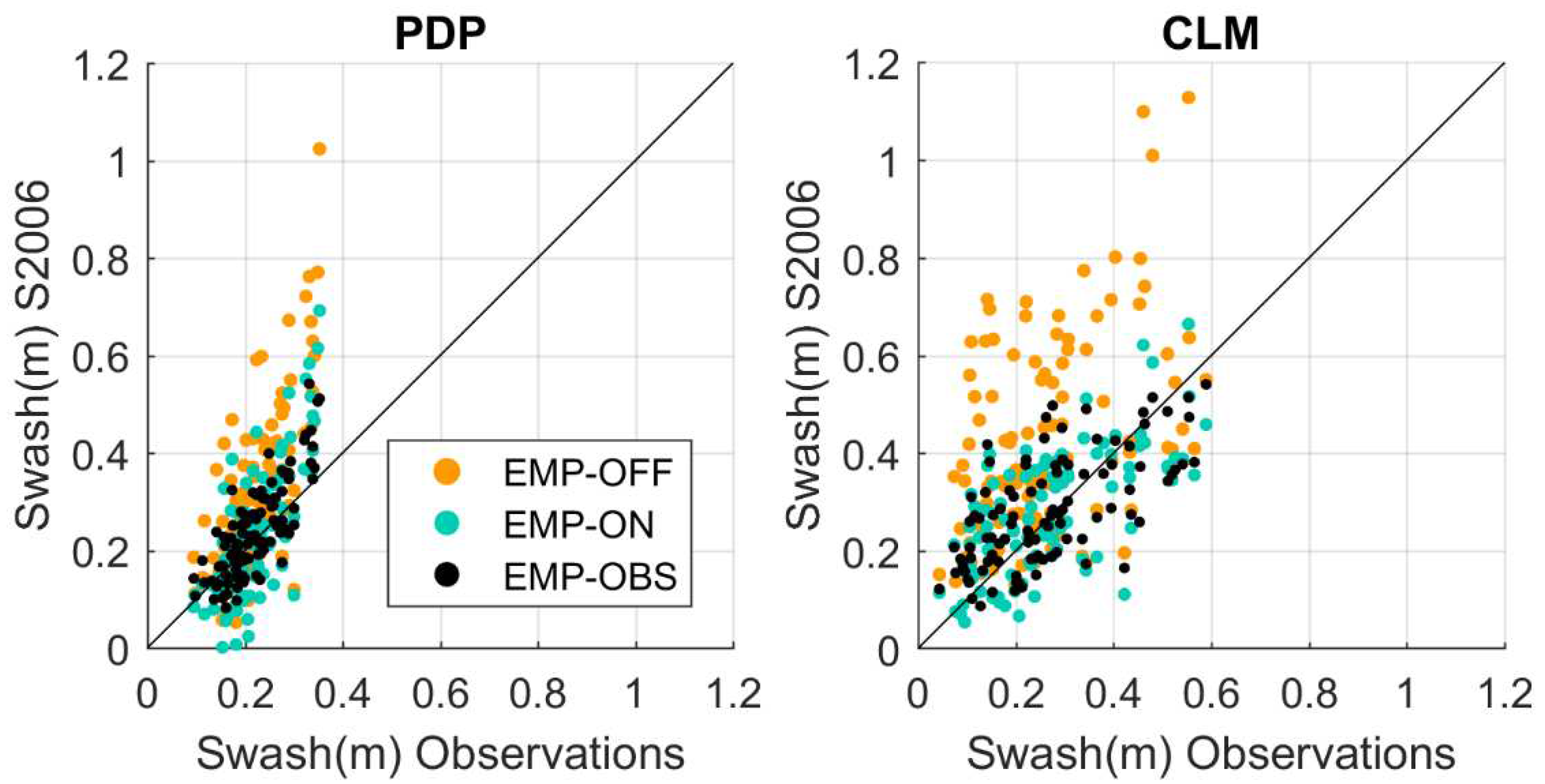
The comparison of the EMP-OFF, EMP-NEAR and EMP-OBS simulations shows that the source of information used to feed the empirical formulation has a significant impact on the swash results (
Figure 5 and
Table 2). Using observed nearshore waves, the RMSE is 0.07 m and 0.11 m for PDP and CLM, respectively. Using modelled nearshore waves, the RMSE increases to 0.09 m in PDP and 0.13 m in CLM. When offshore waves are considered the RMSE reach a maximum value of 0.13 m in PDP and 0.25 m in CLM. Moreover, the representation of the incoming waves also affects the bias (
Table 2). Using observed nearshore waves (either observed or modelled), the bias is almost negligible in both locations. However, if offshore waves are used there is an overestimation of the swash (i.e., the bias reaches 0.07 m in PDP and 0.16 m in CLM).
The RMSE and bias obtained in PDP are lower than those from CLM since PDP is located within an embedded bay, so the offshore and onshore waves are restricted to a range of directions and wave heights which implies smaller swash variability. In contrast, CLM is more exposed to offshore waves coming from different wave directions, so the range of observed swash values increases, and in consequence the RMSE and bias.
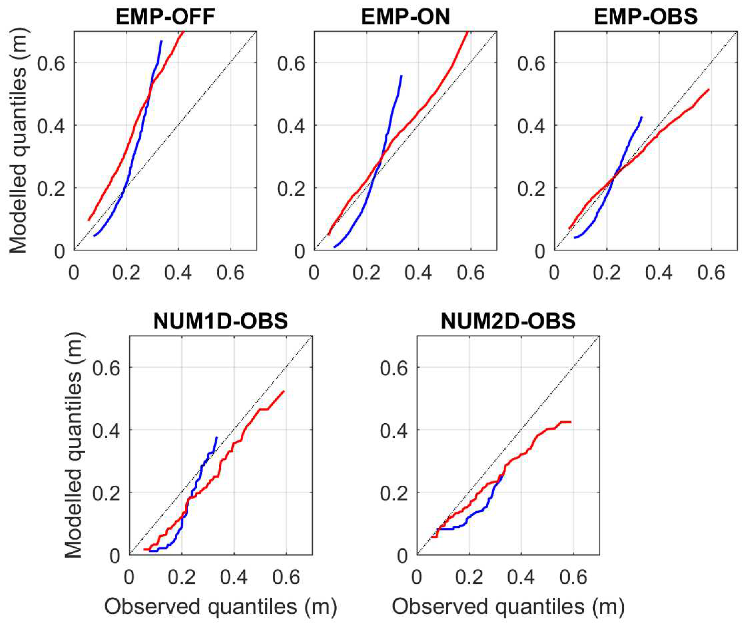
A complementary view can be obtained by looking at the quantile-quantile plots (see
Figure 6). In general, the empirical formulation provides higher values than the observations for all the quantiles with a clear overestimation of the extreme swash values. This is more noticeable in PDP than in CLM.
3.2. Empirical versus Numerical Approaches
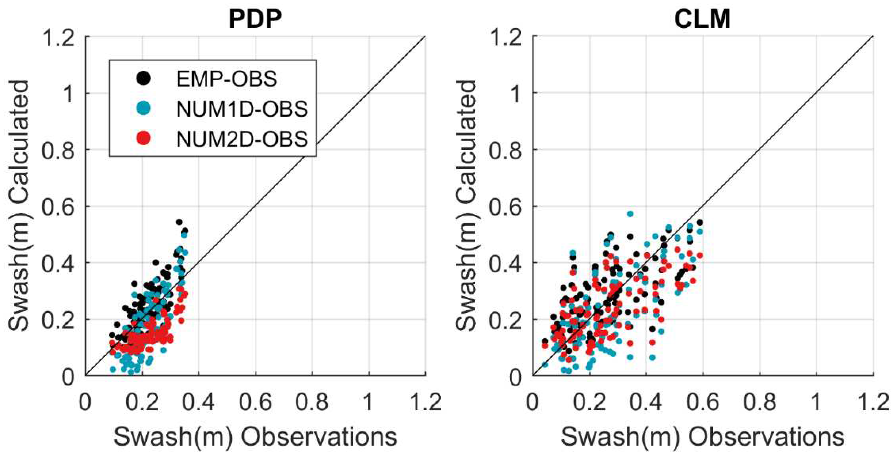
The results obtained using the S2006 formulation fed by observed nearshore waves are similar to those obtained using XBEACH in the 1D or 2D configuration. In PDP, the RMSE are 0.07 m, 0.09 m and 0.07 m, respectively, while in CLM the RMSE are 0.11 m, 0.14 m and 0.12 m (see
Figure 7 and
Table 2). Moreover, the numerical solutions show a negative bias (i.e., underestimates the swash) with values of -0.06 m for both runs in PDP and -0.07 m and -0.04 m for the 1D and 2D runs in CLM, respectively. The results suggest that the numerical approach exhibits similar skills to the simpler empirical formulation. However as discussed later, there is a compensating error in the use of S2006 due to the presence of vegetation. Regarding the quantile-quantile plots (
Figure 6), the results are somehow different in both locations. In PDP, the 1D modelling underestimates the observed swash except for the extreme values, which are correctly represented. Conversely, the 2D modelling also underestimates them. In CLM, the underestimation of the 1D modelling is almost constant and linked to the above-mentioned bias. The 2D modelling, instead, underestimates more the extreme values (about a 30%).
3.3. Sensitivity to Errors in the Bathymetry Slope
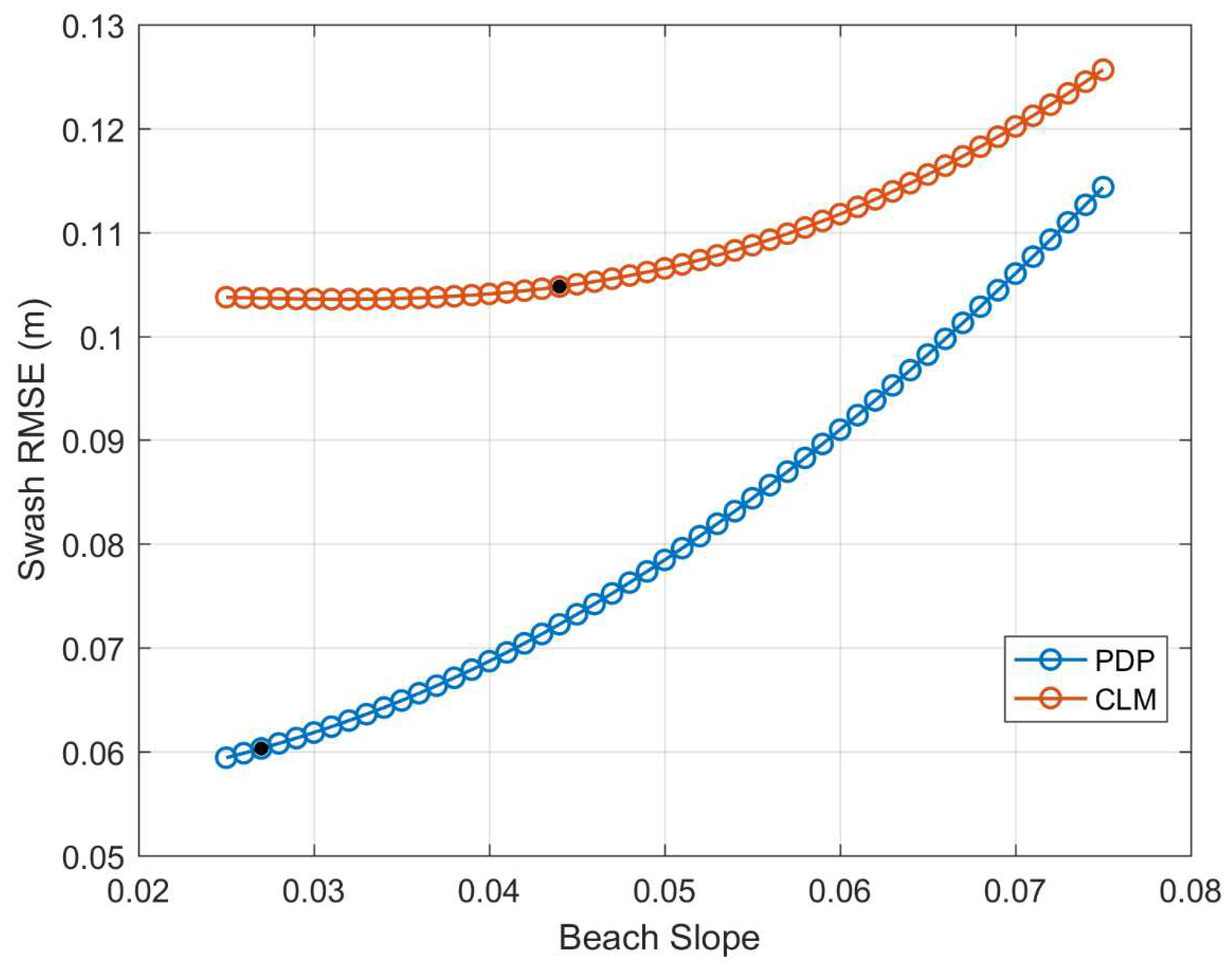
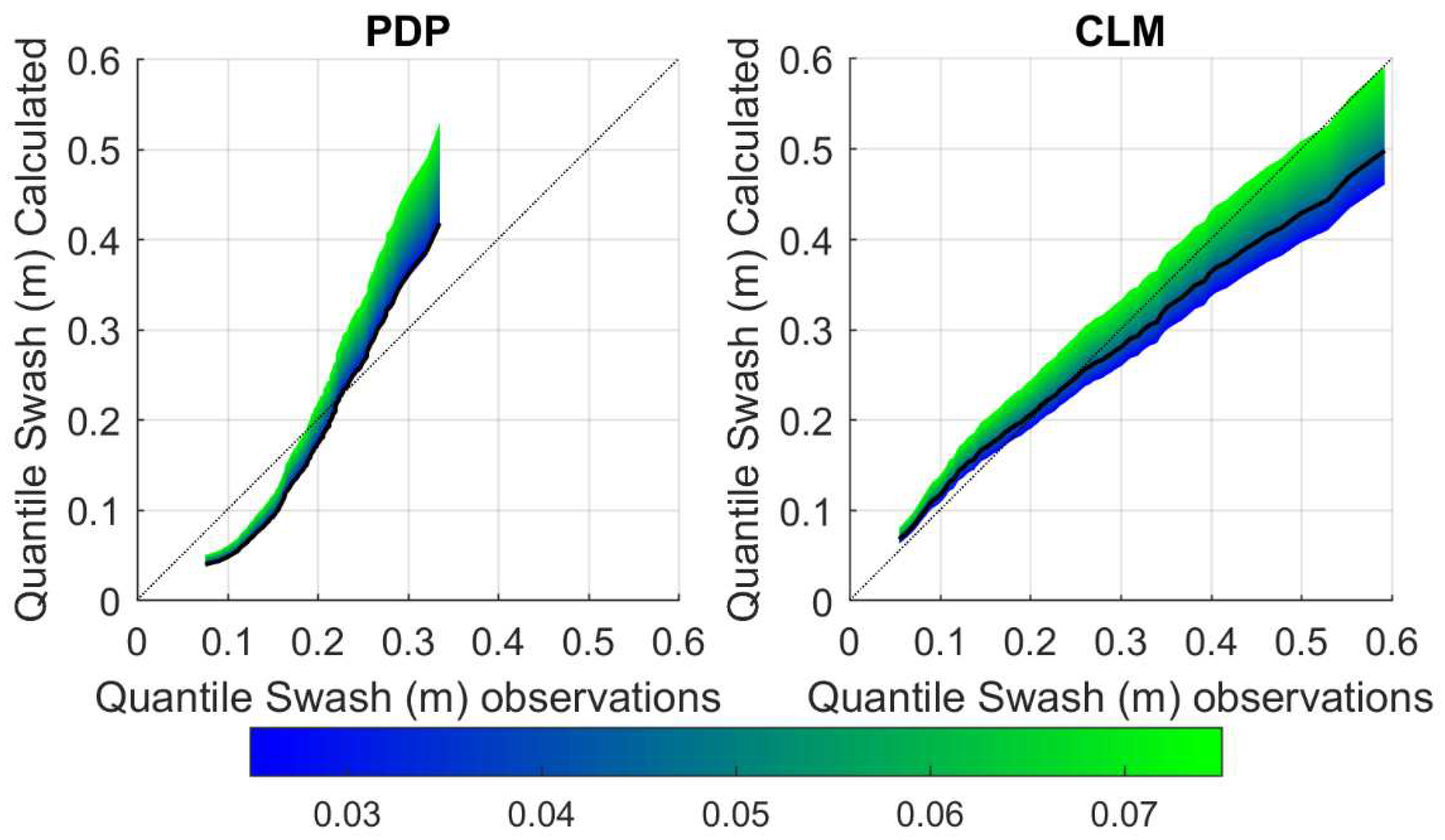
The beach slope have a significant impact on the wave runup estimation (Lange et al., 2022). Aiming at assessing what is the sensitivity of the swash calculation to the bathymetry , we have estimated the range of swash RMSE we obtain using S2006 forced by observed nearshore waves and perturbing the bottom slope from 0.025 to 0.075 (
Figure 8), covering all range of slopes for sandy beaches in the region (Agulles et al., 2021). The results for PDP, where the observed bottom slope is 0.027, show how RMSE would range from 0.06 m to almost the double, 0.11 m. In CLM, where the observed bottom slope is 0.044, the RMSE would increase when using larger slopes, going from 0.11 m to 0.13 m. Compared to the simulation run with the observed slope (EMP-OBS), we see that the RMSE only increases a maximum of 0.02 m. In other words, using an incorrect slope in CLM would result in an increase of less than 20% of the RMSE.
Inaccuracies in the bottom slope would also have an impact on the extreme values (
Figure 9). Namely, using larger slopes lead to larger extreme values in wave runup estimates (equ
$ations (1)–(3)). In PDP, this would imply that the extreme values would be even more overestimated, between 20 % and 40%. In CLM the extreme values are underestimated between -25% using a slope of 0.025 to almost 0% using a slope of 0.075 (
Figure 9).
3.4. Sensitivity to Errors in the Bottom Friction
Several sensitivity runs have been performed forcing the 1D version of Xbeach with observed nearshore waves and changing the bottom drag coefficient due to wave-seagrass interactions (see
Table 3 and Figure SI5). The inclusion of the vegetation module improves the results in both beaches. Without vegetation (FRIC 1), the RMSE is 0.19 m (0.15 m) for PDP (CLM). With the optimal drag coefficient (NUM1D-OBS), the RMSE is reduced to 0.08 m (0.13 m). For the other intermediate cases the results lay in the middle. Using vegetation with Cd= 0.20 the RMSE was 0.13 m (0.17 m) and with Cd=0.10, the RMSE was 0.10 m (0.13 m). Therefore, not considering the submerged vegetation in PDP would more than double the RMSE, while in CLM would represent only a 13% of error increase. Conversely, if the presence of vegetation is taken into account but the characteristics of the vegetation are unknown, and thus the bottom friction is not properly tuned, the resulting RMSE could increase up to 0.05 m in PDP and 0.04 m in CLM.
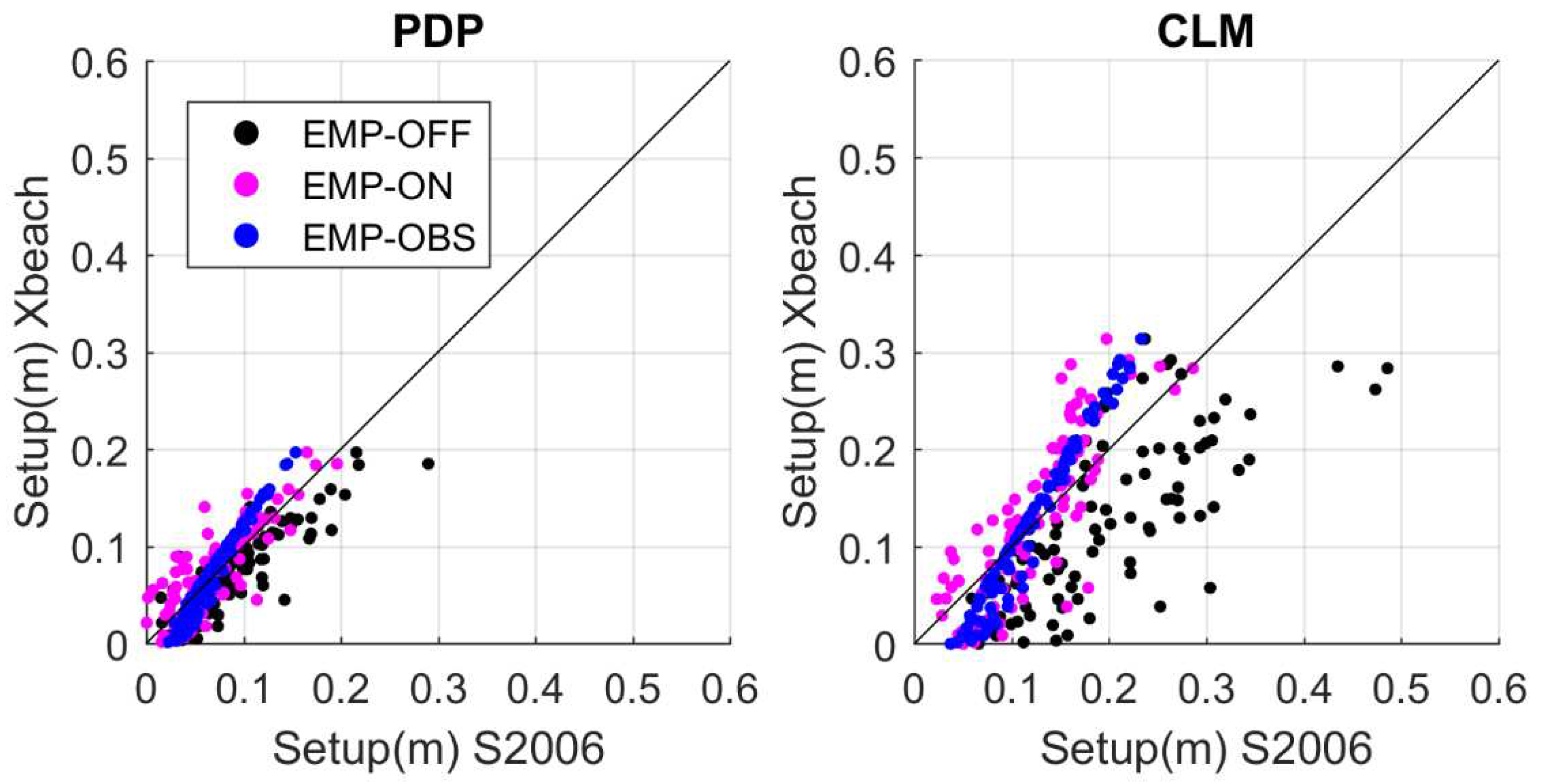
3.5. Sensitivity Analysis of the Wave Setup
As mentioned above, we assume that the wave setup extracted from video imagery is unreliable due to some unquantified processes that could happen on a beach modifying its width (i.e., abrupt erosion under an extreme event, gradually losing or gaining sand or human nourishment). Consequently, here we can only assess the sensitivity of the setup estimation to different configurations. Particularly, we compare the setup provided by the simulations based on S2006 (EMP-OFF, EMP-NEAR and EMP-OBS) with the results from the numerical simulation (NUM2D-OBS, see
Figure 10 and
Table 4). The RMS difference between the numerical and empirical approaches for PDP are 0.03 m, 0.02 m and 0.02 m, respectively. This represents around a 20 % of the RMSE of the swash estimates (
Table 2). In CLM, the RMS difference are 0.10 m, 0.05 m and 0.04 m (~30 % of the RMSE of the swash estimates). As expected, the primary source of discrepancies in the setup estimation is the data source for the waves, as happened for the swash (see
Section 3.1). Namely, using offshore waves induces a large positive bias. Since the setup component has less influence than the swash component on the total runup, the absolute contribution to runup uncertainties remains relatively low.
4. Discussion
The quantification of beach flooding requires the implementation of a modelling system able to propagate the information from open sea waves up to the beach. This can be done using cost-effective empirical approaches or using more sophisticated strategies based on numerical modelling that allows to cope with local specificities. If the runup estimates are needed for a large number of beaches (e.g., in regional assessments), then the second approach is unfeasible. And that is not only because of the computational cost, but also due to the lack of detailed information on nearshore bathymetries and bottom type (e.g. vegetation, sand, rock, etc), which determines the wave damping.
Under some circumstances, using an empirical approach can lead to results comparable to what is obtained with a calibrated numerical model. However, it is worth noting that there may be error compensation. For instance, in our case, the results have shown that the S2006 empirical approach forced with nearshore waves provides similar results than the most sophisticated numerical configuration. At the same time, this approach does not consider the role of vegetation in the wave damping. Therefore, it can be expected that in a location without submerged vegetation close to the shore, the same approach would lead to an underestimation of the observed wave runup. These results are consistent with (Stockdon et al., 2014) in which some modifications to the S2006 formulation were done to improve the wave runup estimates under extreme events.
The quantification of the error sources conducted in this study can help to establish the relative importance of different sources of uncertainty in projections of beach flooding. Those projections will be inherently uncertain for several reasons. Leaving aside that the future evolution of greenhouse gases (GHG) is uncertain and assuming a certain GHG scenario, two other main sources of uncertainty can be identified. These are the natural variability in the forcings and the inaccuracies of the modelling system (Hawkins and Sutton, 2009). In the case of beach flooding, the later can be roughly approximated from the error estimates we have carried out in this study.
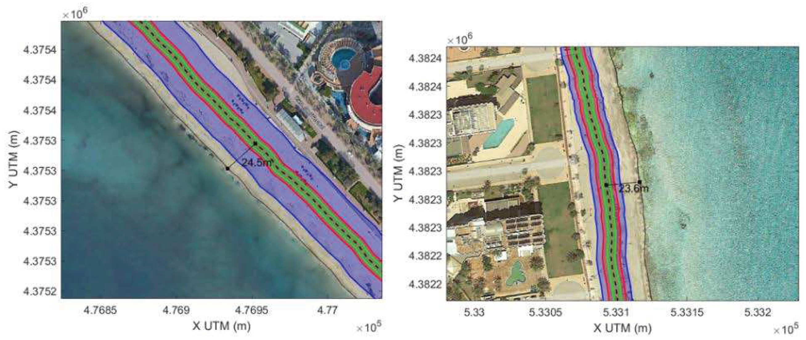
For illustrative purposes, we estimate the uncertainties associated to wave runup computation in a realistic study of beach flooding associated to climate change. For doing that, the baseline is the flood distance projections in the Balearic Islands developed by (Agulles et al., 2021), where projections of mean sea level, storm surges and wave runup evolution are computed along the coast of the archipelago to obtain the flood distance on sandy beaches under different wave conditions and climate scenarios. Based on the results of that work, under the greenhouse gas (GHG) emission scenario RCP8.5, the flood distance under extreme conditions in 2100 in PDP and CLM is projected to be 24.5 m and 23.6 m, respectively (see
Table 1 in Supplementary Material of Agulles et al., 2021). These values can be compared to the uncertainty associated with the wave runup modelling.
The total uncertainties associated to the modelled wave runup could be computed from the uncertainties associated to the swash and the setup. Assuming those are independent and provided that runup is the result of the addition of swash and setup, the wave runup uncertainty (e
runup) can be estimated as the quadratic sum of the uncertainties in each component (Kirchner, 2001; Ranftl et al., 2021), which results in:
The uncertainties linked to the modelling of the swash can be estimated from the errors quantified above. Regarding the uncertainties in the setup, we can use the RMS difference of the sensitivity study shown in
Section 3.5. Both uncertainties would depend on the modelling approach. In the case where the 2D numerical approach is implemented with observed 2D bathymetry and vegetation and forced with observed nearshore waves (NUM2D-OBS), the swash results would have an uncertainty similar to the baseline swash error (0.07 m for PDP), and the setup results would have an uncertainty similar to the baseline setup error (0.02 m, for PDP; here we use the minimum RMSD of
Table 4). Thus, from (4), the uncertainty in the vertical runup in PDP would be 0.07 m. Considering that the PDP beach slope is 0.027, this value corresponds to an uncertainty of 2.70 m for the horizontal displacement. The same configuration for CLM would have an uncertainty in the wave swash and setup of 0.12 m and 0.04 m, respectively. This leads to an uncertainty in the wave runup of 0.13 m and 2.95 m in the flood distance assuming a beach slope of 0.044 (
Table 5). Thus, the uncertainties associated to the wave runup modelling corresponds to a 11% and 12% of the total flood distance estimated by Agulles et al (2021) (green patch in
Figure 11) for PDP and CLM, respectively.
A second example would be the case of most regional studies, where wave run up is estimated from the empirical formulation of S2006 with offshore waves and little knowledge on bathymetry or vegetation. In this case, we should add the uncertainty in the swash and setup due to the use of offshore waves with the empirical formulation, the unknown bathymetry and the unknown bottom friction. Once again, we can assume that the distinct sources of uncertainty are independent and we can combine them as a quadratic sum. For PDP, we assume that the uncertainty linked to the first can be approximated by the estimated error of EMP-OFF run in
Table 2 (0.13 m in PDP and 0.25 m in CLM). The uncertainty due to the unknown bathymetry can be approximated from the results of the sensitivity experiments (section 3.3). There, we have seen that using a wrong bathymetric slope would lead to an increase of 0.02 m in both beaches. For the uncertainty linked to the vegetation, we can use an average value from the results of sensitivity experiments in section 3.4 and assume an uncertainty of 0.08 m in PDP and 0.02 in CLM. Finally, we use again the results of the comparison of wave setup results from section 3.5 for the uncertainty linked to the wave setup (0.03 m for PDP and 0.10 m for CLM). Merging all sources of uncertainty leads to a total uncertainty in the vertical displacement of 0.16 m for PDP and 0.27 m for CLM. The corresponding uncertainty in the horizontal displacement would be 5.80 m and 6.15 m, respectively (see
Table 5). Thus, the uncertainties associated to the modelling of wave runup using the simplest configuration (EMP-OFF) correspond to a 23% and 26% of the total flood distance estimated by Agulles et al (2021) (green patch in
Figure 11) for PDP and CLM, respectively.
It is also worthwhile to compare the uncertainties associated to the modelling of wave runup with the other sources of uncertainty for beach flooding projections. In particular, in the Mediterranean, most of the uncertainties linked to beach flooding projections are associated to the representation of changes in the mean sea level, as storm surge and open sea waves are well modelled and projected to suffer minor changes (Agulles et al., 2021). Previous studies have quantified the uncertainties in mean sea level projections associated to the scenario or the modelling system. They suggest mean sea level will rise between 0.20 and 1.10 m at the end of the century (Cherif et al., 2020; Zhongming et al., 2021). Thus, the uncertainty in mean sea level projections would be ~0.45 m. Our results suggest that uncertainties associated to the modelling of wave runup would be between 0.07 m and 0.27 m depending on the beach studied and the modelling choices, which represents between a 16 % and 60 % of the uncertainties linked to the mean sea level projections (see Figure 12). This means that uncertainties associated to the wave runup modelling are important and thus should not be neglected when estimating total uncertainties of the beach flooding projections.
5. Conclusions
In this paper, we have quantified the impact of several sources of error in the estimation of wave runup in sandy beaches to assess what factors have a greater influence on the quality of the results. To reach that goal, a calibrated state-of-the-art numerical modelling system has been setup for two beaches in the Mallorca islands (NW Mediterranean), which are representative of most Mediterranean sandy beaches. The system has been forced with the best available information of nearshore incoming waves and has been validated against swash observations to define the benchmark quality. Then different system configurations have been tested with different degrees of complexity.
Our results show that using the most sophisticated modelling system with the best information on boundary conditions, bottom bathymetry, and submerged vegetation leads to a swash RMSE comparable to the standard deviation of the observed swash. We have also found that the choice of lateral boundary conditions (i.e., source of information for the incoming waves) is the most influential factor and can double the RMSE and induce large biases. The second factor in importance is if submerged vegetation is properly considered or not as it modifies the nearshore wave damping. The comparison between different modelling approaches also demonstrates that employing a simple empirical approach typically underestimates wave runup. Nevertheless, in areas with vegetated seabed, there is an error compensation, and the empirical approach can yield acceptable outcomes if forced by nearshore waves.
The quantification of the sources of error for wave runup estimates can also help to assess the relative importance of the uncertainty associated with the wave runup modelling when projecting future evolution of total water level at beaches. To illustrate this, the projections of beach flooding under scenario RCP8.5 have been used as an example. Assuming that the uncertainties of modelling wave runup can be approximated by the error estimates presented above, those would range between 0.07 m and 0.27 m depending on the beach studied and the modelling choices. Those uncertainties in wave runup represents between 16 % and 60% of the uncertainties associated to the mean sea level rise projections in the region. Therefore, uncertainties associated to wave runup modelling should be considered when assessing the uncertainties associated to beach flooding projections. These outcomes can be extrapolated to other Mediterranean beaches with similar morphodynamical characteristics.
Supplementary Materials
The following supporting information can be downloaded at the website of this paper posted on Preprints.org, Figure SI1. Swash observations extracted from timestack images (blue bars). Setup from S2006 formulation (red bars) and XBEACH (green bars), both for PDP (top) and CLM (bottom panel). The sum of both components represents the wave runup (in m). Figure SI2. Time series of nearshore waves recorded by the AWACS (gray) and the selected cases modelled by XBEACH (green and red dots). The black dots indicate the periods when timestack images were available. Figure SI3. Scatter plot of modelled Hs (m) with SWAN vs observations in PDP (left panel) and CLM (right panel). Figure SI4. Validation of the XBEACH model outputs in Cala Millor along a cross-shore transect of wave observations by Infantes et al., (2012). The location of the wave observations is indicated by the red dots (P1 to P4) in the upper panel. The lower panels show the comparison of observed and modelled Hrms (in m) for the four observation points. The corresponding RMSE (in m) is included in the insets for the simulation with the calibrated vegetation module (R). Figure SI5. Calibration of XBEACH vegetation module for PDP (left panel) and SNB (right panel). Observed and modelled swash are compared in the absence of seagrass (blue), considering Cd=0.20 (green), Cd=0.10 (red) and Cd=0.05 (black).
Credit authorship contribution statement
Miguel Agulles: Conceptualization, Methodology, Validation, Formal analysis, Investigation and writing. Gabriel Jordà: Conceptualization, Investigation, writing-review and editing, Project administration and Funding acquisition.
Acknowledgments
The authors would like to thank Puertos del Estado for the data provided, SOCIB for the data provided as the assistance of Àngels Fernández Mora. We also would like to express our appreciation to CSIC-IEO institution for providing the necessary infrastructure to carry out this work in the best conditions. This work is part of the R+D+I projects VENOM (PGC2018-099285-B-C22), and UNCHAIN (PCI2019-103680) funded by MCIN/AEI/10.13039/501100011033 and by ERDF A way of making Europe.
Declaration of competing interest
The authors declare that they have no known competing financial interests or personal relationships that could have appeared to influence the work reported in this paper.
References
- Agulles: M., Jordà, G., Lionello, P., 2021. Flooding of Sandy Beaches in a Changing Climate. The Case of the Balearic Islands (NW Mediterranean). Frontiers in Marine Science 8, 1–15. [CrossRef]
- Alvarez-ellacuria, A., Or, A., Gómez-pujol, L., Simarro, G., Obregon, N., 2011. Geomorphology Decoupling spatial and temporal patterns in short-term beach shoreline response to wave climate 128, 199–208. [CrossRef]
- Amores, A., Marcos, M., Carrió, D.S., Gómez-Pujol, L., 2020. Coastal impacts of Storm Gloria (January 2020) over the north-western Mediterranean. Natural Hazards and Earth System Sciences 20, 1955–1968. [CrossRef]
- Atkinson, A.L., Power, H.E., Moura, T., Hammond, T., Callaghan, D.P., Baldock, T.E., 2017. Assessment of runup predictions by empirical models on non-truncated beaches on the south-east Australian coast. Coastal Engineering 119, 15–31. [CrossRef]
- Beck, M.W., Losada, I.J., Menéndez, P., Reguero, B.G., Díaz-Simal, P., Fernández, F., 2018. The global flood protection savings provided by coral reefs. Nature Communications 9. [CrossRef]
- Blackwell, B.D., Raybould, M., Lazarow, N., 2013. Beaches as societal assets: Council expenditures, recreational returns, and climate change. Handbook of Tourism Economics: Analysis, New Applications and Case Studies 443–467. [CrossRef]
- Booij, N., Holthuijsen, L.H., 1987. Propagation of ocean waves in discrete spectral wave models. Journal of Computational Physics 68, 307–326. [CrossRef]
- Camus, P., Mendez, F.J., Medina, R., Cofiño, A.S., 2011. Analysis of clustering and selection algorithms for the study of multivariate wave climate. Coastal Engineering 58, 453–462. [CrossRef]
- Camus, P., Mendez, F.J., Medina, R., Tomas, A., Izaguirre, C., 2013. High resolution downscaled ocean waves (DOW) reanalysis in coastal areas. Coastal Engineering 72, 56–68. [CrossRef]
- Cebrián, J., Duarte, C.M., Marbà, N., Enríquez, S., Gallegos, M., Olesen, B., 1996. Herbivory on Posidonia oceanica: Magnitude and variability in the Spanish Mediterranean. Marine Ecology Progress Series 130, 147–155. [CrossRef]
- Cherif, S., Doblas-Miranda, E., Lionello, P., Borrego, C., Giorgi, F., Iglesias, A., Jebari, S., Mahmoudi, E., Moriondo, M., Pringault, O., Rilov, G., Somot, S., Tsikliras, A., Vila, M., Zittis, G., 2020. Chapter 2 Drivers of Change. Climate and Environmental Change in the Mediterranean Basin – Current Situation and Risks for the Future. First Mediterranean Assessment Report 1–26.
- Cobb, K.M., Rojas, M., Chen, D., Samset, B.H., Diongue-Niang, A., Edwards, P.N., Emori, S., Hawkins, E., Faria, S.H., Hope, P., 2021. Framing, context, and methods, in: AGU Fall Meeting 2021. AGU.
- de los Santos, C.B., Krause-Jensen, D., Alcoverro, T., Marbà, N., Duarte, C.M., van Katwijk, M.M., Pérez, M., Romero, J., Sánchez-Lizaso, J.L., Roca, G., Jankowska, E., Pérez-Lloréns, J.L., Fournier, J., Montefalcone, M., Pergent, G., Ruiz, J.M., Cabaço, S., Cook, K., Wilkes, R.J., Moy, F.E., Trayter, G.M.R., Arañó, X.S., de Jong, D.J., Fernández-Torquemada, Y., Auby, I., Vergara, J.J., Santos, R., 2019. Recent trend reversal for declining European seagrass meadows. Nature Communications 10, 1–8. [CrossRef]
- Di Luccio, D., Benassai, G., Budillon, G., Mucerino, L., Montella, R., Pugliese Carratelli, E., 2018. Wave run-up prediction and observation in a micro-tidal beach. Natural Hazards and Earth System Sciences 18, 2841–2857. [CrossRef]
- Didier, D., Bernatchez, P., Boucher-Brossard, G., Lambert, A., Fraser, C., Barnett, R.L., Van-Wierts, S., 2015. Coastal flood assessment based on field debris measurements and wave runup empirical model. Journal of Marine Science and Engineering 3, 560–590. [CrossRef]
- Duarte, C.M., Losada, I.J., Hendriks, I.E., Mazarrasa, I., Marbà, N., 2013. The role of coastal plant communities for climate change mitigation and adaptation. Nature Climate Change 3, 961–968. [CrossRef]
- Enríquez, A.R., Marcos, M., Álvarez-Ellacuría, A., Orfila, A., Gomis, D., 2017. Changes in beach shoreline due to sea level rise and waves under climate change scenarios: Application to the Balearic Islands (western Mediterranean). Natural Hazards and Earth System Sciences 17, 1075–1089. [CrossRef]
- Enríquez, A.R., Marcos, M., Falqués, A., Roelvink, D., 2019. Assessing beach and dune erosion and vulnerability under sea level rise: A Case study in the Mediterranean Sea. Frontiers in Marine Science 6, 1–12. [CrossRef]
- Giorgi, F., 2010. Uncertainties in climate change projections, from the global to the regional scale. EPJ Web of Conferences 9, 115–129. [CrossRef]
- Gomes da Silva, P., Coco, G., Garnier, R., Klein, A.H.F., 2020. On the prediction of runup, setup and swash on beaches. Earth-Science Reviews 204, 103148. [CrossRef]
- Gomes da Silva, P., Medina, R., González, M., Garnier, R., 2018. Infragravity swash parameterization on beaches: The role of the profile shape and the morphodynamic beach state. Coastal Engineering 136, 41–55. [CrossRef]
- Gómez-pujol, L., Or, A., Álvarez-ellacuría, A., Tintoré, J., 2011. Geomorphology Controls on sediment dynamics and medium-term morphological change in a barred microtidal beach ( Cala Millor , Mallorca , Western Mediterranean ) 132, 87–98. [CrossRef]
- Harley, M., Armaroli, C., Ciavola, P., 2011. Evaluation of XBeach predictions for a real-time warning system in Emilia-Romagna, Northern Italy. Journal of Coastal Research 1861–1865.
- Hasselmann, K., Hasselmann, S., Bauer, E., Janssen, P.A.E.M., Komen, G.J., Bertotti, L., Lionello, P., Guillaume, A., Cardone, V.C., Greenwood, J.A., Reistad, M., Zambresky, L., Ewing, J.A., 1988. The WAM model - a third generation ocean wave prediction model. J. Phys. Oceanogr. 18, 1775–1810. [CrossRef]
- Hawkins, E., Sutton, R., 2009. The potential to narrow uncertainty in regional climate predictions. Bulletin of the American Meteorological Society 90, 1095–1108. [CrossRef]
- Holman, R.A., 1986. Extreme value statistics for wave run-up on a natural beach. Coastal Engineering 9, 527–544. [CrossRef]
- Holman, R.A., Guza, R.T., 1984. Measuring run-up on a natural beach. Coastal Engineering 8, 129–140. [CrossRef]
- Horton, B.P., Khan, N.S., Cahill, N., Lee, J.S.H., Shaw, T.A., Garner, A.J., Kemp, A.C., Engelhart, S.E., Rahmstorf, S., 2020. Estimating global mean sea-level rise and its uncertainties by 2100 and 2300 from an expert survey. npj Climate and Atmospheric Science 3, 1–8. [CrossRef]
- Infantes, E., Orfila, A., Simarro, G., Terrados, J., Luhar, M., Nepf, H., 2012. Effect of a seagrass (Posidonia oceanica) meadow on wave propagation. Marine Ecology Progress Series 456, 63–72. [CrossRef]
- Kirchner, J., 2001. Data analysis toolkit# 5: uncertainty analysis and error propagation. University of California Berkeley Seismological Laboratory. Available online at: http://seismo. berkeley. edu/~ kirchner/eps_120/Toolkits/Toolkit_05. pdf.
- Lange, A.M.Z., Fiedler, J.W., Becker, J.M., Merrifield, M.A., Guza, R.T., 2022. Estimating runup with limited bathymetry ✩. Coastal Engineering 172, 104055. [CrossRef]
- Marcos, M., Tsimplis, M.N., 2007. Forcing of coastal sea level rise patterns in the North Atlantic and the Mediterranean Sea. Geophysical Research Letters 34. [CrossRef]
- Mejjad, N., Rossi, A., Pavel, A.B., 2022. The coastal tourism industry in the Mediterranean: A critical review of the socio-economic and environmental pressures & impacts. Tourism Management Perspectives 44, 101007. [CrossRef]
- Mendez, F.J., Losada, I.J., 2004. An empirical model to estimate the propagation of random breaking and nonbreaking waves over vegetation fields. Coastal Engineering 51, 103–118. [CrossRef]
- Menéndez, P., Losada, I.J., Torres-Ortega, S., Narayan, S., Beck, M.W., 2020. The Global Flood Protection Benefits of Mangroves. Scientific Reports 10. [CrossRef]
- Oddo, P.C., Lee, B.S., Garner, G.G., Srikrishnan, V., Reed, P.M., Forest, C.E., Keller, K., 2020. Deep Uncertainties in Sea-Level Rise and Storm Surge Projections: Implications for Coastal Flood Risk Management. Risk Analysis 40, 153–168. [CrossRef]
- Orejarena-Rondón, A.F., Sayol, J.M., Marcos, M., Otero, L., Restrepo, J.C., Hernández-Carrasco, I., Orfila, A., 2019. Coastal Impacts Driven by Sea-Level Rise in Cartagena de Indias. Frontiers in Marine Science 6. [CrossRef]
- Pilar, P., Soares, C.G., Carretero, J.C., 2008. 44-year wave hindcast for the North East Atlantic European coast. Coastal Engineering 55, 861–871. [CrossRef]
- Ranftl, S., von der Linden, W., Committee, M. 2021 S., 2021. Bayesian surrogate analysis and uncertainty propagation, in: Physical Sciences Forum. MDPI, p. 6. [CrossRef]
- Roelvink, D., McCall, R., Mehvar, S., Nederhoff, K., Dastgheib, A., 2018. Improving predictions of swash dynamics in XBeach: The role of groupiness and incident-band runup. Coastal Engineering 134, 103–123. [CrossRef]
- Roelvink, D., van Dongeren, A., McCall, R., Hoonhout, B., van Rooijen, A., van Geer, P., de Vet, L., Nederhoff, K., Quataert, E., 2015. XBeach Technical Reference : Kingsday Release 1–141. [CrossRef]
- Ruiz, J.M., Guillén, E., Ramos Segura, A., Otero, M., 2015. Atlas de las praderas marinas de España. Instituto Español de Oceanografía.
- Satta, A., Puddu, M., Venturini, S., Giupponi, C., 2017. Assessment of coastal risks to climate change related impacts at the regional scale: The case of the Mediterranean region. International Journal of Disaster Risk Reduction 24, 284–296. [CrossRef]
- Simarro, G., Ribas, F., Álvarez, A., Guillén, J., Chic, Ò., Orfila, A., 2017. ULISES: An Open Source Code for Extrinsic Calibrations and Planview Generations in Coastal Video Monitoring Systems. Journal of Coastal Research 335, 1217–1227. [CrossRef]
- Stockdon, H.F., Holman, R.A., Howd, P.A., Sallenger, A.H., 2006. Empirical parameterization of setup, swash, and runup. Coastal Engineering 53, 573–588. [CrossRef]
- Stockdon, H.F., Thompson, D.M., Plant, N.G., Long, J.W., 2014. Evaluation of wave runup predictions from numerical and parametric models. Coastal Engineering 92, 1–11. [CrossRef]
- Telesca, L., Belluscio, A., Criscoli, A., Ardizzone, G., Apostolaki, E.T., Fraschetti, S., Gristina, M., Knittweis, L., Martin, C.S., Pergent, G., Alagna, A., Badalamenti, F., Garofalo, G., Gerakaris, V., Louise Pace, M., Pergent-Martini, C., Salomidi, M., 2015. Seagrass meadows (Posidonia oceanica) distribution and trajectories of change. Scientific Reports 5, 1–14. [CrossRef]
- Tintoré, J., Vizoso, G., Las Casas, G., Heslop, E., Pascual, A., Orfila, A., Ruiz, S., Martínez-Ledesma, M., Torner, M., Cusi, S., Diedrich, A., Balaguer Huguet, P., Gómez-Pujol, L., Álvarez-Ellacuria, A., Gómara, S., Sebastian, K., Lora, S., Beltrán, J., Renault, L., Manriquez, M., 2013. SOCIB: The Balearic Islands Coastal Ocean Observing and Forecasting System Responding to Science, Technology and Society Needs. Marine Technology Society Journal 47, 101–117. [CrossRef]
- Tsimplis, M.N., Proctor, R., Flather, R.A., 1995. A two-dimensional tidal model for the Mediterranean Sea. Journal of Geophysical Research: Oceans 100, 16223–16239. [CrossRef]
- van Rooijen, A.A., van Thiel de Vries, J.S.M., McCall, R.T., van Dongeren, A.R., Roelvink, J.A., Reniers, A.J.H.M., 2015. Modeling of wave attenuation by vegetation with XBeach. E-proceedings of the 36th IAHR World Congress 7.
- Vousdoukas, Michalis I., Ferreira, Ó., Almeida, L.P., Pacheco, A., 2012. Toward reliable storm-hazard forecasts: XBeach calibration and its potential application in an operational early-warning system. Ocean Dynamics 62, 1001–1015. [CrossRef]
- Vousdoukas, M.I., Ranasinghe, R., Mentaschi, L., Plomaritis, T.A., Athanasiou, P., Luijendijk, A., Feyen, L., 2020. Sandy coastlines under threat of erosion. Nature Climate Change 10, 260–263. [CrossRef]
- Vousdoukas, Michalis Ioannis, Wziatek, D., Almeida, L.P., 2012. Coastal vulnerability assessment based on video wave run-up observations at a mesotidal, steep-sloped beach. Ocean Dynamics 62, 123–137. [CrossRef]
- Xie, D., Zou, Q.P., Mignone, A., MacRae, J.D., 2019. Coastal flooding from wave overtopping and sea level rise adaptation in the northeastern USA. Coastal Engineering 150, 39–58. [CrossRef]
- Zhongming, Z., Linong, L., Xiaona, Y., Wangqiang, Z., Wei, L., 2021. AR6 Climate Change 2021: The Physical Science Basis.
- Zijlema, M., Stelling, G., Smit, P., 2011. SWASH: An operational public domain code for simulating wave fields and rapidly varied flows in coastal waters. Coastal Engineering 58, 992–1012. [CrossRef]
Figure 1.
Left panel, location of the study sites with the position of the onshore wave observations (orange dots), SIMAR points (yellow dots) and SWAN grids (gray dashed rectangles). (a) Detailed view of Playa de Palma beach (PDP) with the transects considered to obtain a representative beach profile (yellow dashed lines), (b) the same for Cala Millor Beach (CLM). A sketch of the modelling approach is presented in the right panel.
Figure 2.
Wave maritime climate conditions for (a) Playa de Palma Beach and (b) Cala Millor Beach. The panels represent a scatter plot of Hs (in m) vs Tp (in s), left column, and Hs (in m) vs Direction (º), right column. The offshore conditions are represented by the grey dots while the observed nearshore conditions are represented by the coloured dots, with the colour representing the frequency of occurrence.
Figure 3.
Beach profile at PDP (red) and CLM (green). Seasonal profiles (dashed lines) and annual mean profile (continuous lines). Green patches represent the presence of seagrass meadows.
Figure 3.
Beach profile at PDP (red) and CLM (green). Seasonal profiles (dashed lines) and annual mean profile (continuous lines). Green patches represent the presence of seagrass meadows.
Figure 4.
(Top) Runup timestack generated with the time sequence of cross-shore pixels for day 7th of January 2016. (Bottom) Zoom of the swash zone limited by the dashed red line in the top panel. Runup and rundown are showed as a black edge moving back and forth in the swash zone. The 98% quantile of the swash (yellow line) and swash mean value (white dashed line) are also plotted.
Figure 5.
Scatter plot of swash observations versus swash estimated using the S2006 formulation with different wave forcings in the Playa de Palma (left) and Cala Millor (right). The offshore waves (EMP-OFF run, yellow dots), nearshore modelled waves (EMP-NEAR run, green dots) and nearshore observed waves (EMP-OBS run, black dots) have been used.
Figure 6.
Comparison of observed and modelled quantiles for different simulations. Each subplot depicts the results of PDP (blue) and CLM (red).
Figure 6.
Comparison of observed and modelled quantiles for different simulations. Each subplot depicts the results of PDP (blue) and CLM (red).
Figure 7.
Scatter plot of swash observations versus swash estimated using the S2006 formulation (black), XBEACH-1D (blue) and XBEACH-2D (red) in the Playa de Palma (left) and Cala Millor (right). In all cases observed nearshore waves have been used to force the models.
Figure 7.
Scatter plot of swash observations versus swash estimated using the S2006 formulation (black), XBEACH-1D (blue) and XBEACH-2D (red) in the Playa de Palma (left) and Cala Millor (right). In all cases observed nearshore waves have been used to force the models.
Figure 8.
Swash RMSE (in m) using S2006 formulation with a range of values for the beach slope for PDP (blue) and CLM (red). The black cercles indicate the RMSE corresponding to the observed slopes.
Figure 8.
Swash RMSE (in m) using S2006 formulation with a range of values for the beach slope for PDP (blue) and CLM (red). The black cercles indicate the RMSE corresponding to the observed slopes.
Figure 9.
Comparison of observed and modelled quantiles using the S2006 formulation with a range of values for the beach slope for PDP (left) and CLM (right). The black line indicates the results obtained with the observed beach slope.
Figure 9.
Comparison of observed and modelled quantiles using the S2006 formulation with a range of values for the beach slope for PDP (left) and CLM (right). The black line indicates the results obtained with the observed beach slope.
Figure 10.
Comparison of wave setup between XBEACH (NUM1D-OBS run) and the empirical approach fed by offshore waves (black dots), modelled nearshore waves (magenta dots) and observed nearshore waves (blue dots) in PDP (left) and CLM (right).
Figure 10.
Comparison of wave setup between XBEACH (NUM1D-OBS run) and the empirical approach fed by offshore waves (black dots), modelled nearshore waves (magenta dots) and observed nearshore waves (blue dots) in PDP (left) and CLM (right).
Figure 11.
Example of uncertainties in coastal retreat projected for PDP (left panel) and CLM (right panel). The present location of the coastline is plotted in black. The projected retreat at the end of the century under scenario RCP8.5 is plotted in black dashed line and their associated uncertainties represented by the blue patch. The uncertainty associated to the wave runup estimate is plotted in red for the configuration 1 and in green for the configuration 2 (see text for details).
Table 1.
List of simulations performed with the model, bathymetry and the wave forcing used.
Table 1.
List of simulations performed with the model, bathymetry and the wave forcing used.
| RUN |
MODEL |
WAVE FORCING |
BATHYMETRY |
| 1. EMP-OFF |
Empirical – S2006 |
Offshore Modelled (SIMAR) |
Observed Slope |
| 2. EMP-ON |
Empirical – S2006 |
Onshore Modelled (SWAN) |
Observed Slope |
| 3. EMP-OBS |
Empirical – S2006 |
Onshore observations (AWAC) |
Observed Slope |
| 4.NUM1D-OBS |
Numerical XBEACH-1D |
Onshore observations (AWAC) |
Observed Profile |
| 5.NUM2D-OBS |
Numerical XBEACH-2D |
Onshore observations (AWAC) |
Observed 2D bathymetry |
| 6. BATHY |
Empirical – S2006 |
Onshore observations (AWAC) |
Varying Slope |
| 7. FRIC |
Numerical XBEACH-1D |
Onshore observations (AWAC) |
Varying vegetation |
Table 2.
Validation of the swash obtained from different simulations against observations in terms of RMSE (in m) and bias (in m) for PDP and CLM.
Table 2.
Validation of the swash obtained from different simulations against observations in terms of RMSE (in m) and bias (in m) for PDP and CLM.
| |
PDP |
CLM |
| RMSD (m) |
BIAS (m) |
RMSD (m) |
BIAS (m) |
| EMP-OFF |
0.13 |
0.07 |
0.25 |
0.16 |
| EMP-ON |
0.09 |
0.00 |
0.13 |
0.03 |
| EMP-OBS |
0.07 |
0.01 |
0.11 |
0.00 |
| NUM1D-OBS |
0.09 |
-0.06 |
0.14 |
-0.07 |
| NUM2D-OBS |
0.07 |
-0.06 |
0.12 |
-0.04 |
Table 3.
Parameters used in the sensitivity tests for the drag coefficient calibration and results of the validation in terms of RMSE (in m). The parameters considered are the mean shoot length (Ah), stem width (Bv), vegetation density (N) and drag coefficient (Cd). The symbol (-) indicates that no vegetation module has been included in the XBEACH simulations.
| Tests |
Ah (m) |
Bv (m) |
N (shoots/m2) |
Cd |
RMSE (m) |
| PDP |
CLM |
| FRIC 1 |
- |
- |
- |
- |
0.19 |
0.15 |
| FRIC 2 |
0.35 |
0.02 |
615 |
0.20 |
0.13 |
0.17 |
| FRIC 3 |
0.35 |
0.02 |
615 |
0.10 |
0.10 |
0.13 |
| NUM1D-OBS |
0.35 |
0.02 |
615 |
0.05 |
0.08 |
0.13 |
Table 4.
Comparison of the setup obtained from the empirical approaches with the one provided by NUM2D-OBS in terms of RMS difference (in m) and bias (in m).
Table 4.
Comparison of the setup obtained from the empirical approaches with the one provided by NUM2D-OBS in terms of RMS difference (in m) and bias (in m).
| |
PDP |
CLM |
| RMSD (m) |
BIAS (m) |
RMSD (m) |
BIAS (m) |
| EMP-OFF |
0.03 |
0.02 |
0.10 |
0.08 |
| EMP-ON |
0.02 |
0.00 |
0.05 |
0.02 |
| EMP-OBS |
0.02 |
0.01 |
0.04 |
0.01 |
Table 5.
Total uncertainties in the vertical swash, setup, wave runup and the horizontal coastline displacement. In Configuration 1, a 2D numerical system with good knowledge on bathymetry and vegetation and forced by observed waves has been considered. In Configuration 2 an empirical formulation with poor knowledge on the bathymetry or vegetation and forced by offshore modelled waves has been considered.
| |
Configuration 1 (NUM2D-OBS) |
Configuration 2 (EMP-OFF) |
| |
PDP(β=0.027) |
CLM(β=0.044) |
PDP(β=0.027) |
CLM(β=0.044) |
| Vertical uncertainties |
| Swash (m) |
0.07 |
0.12 |
0.15 |
0.25 |
| Setup (m) |
0.02 |
0.04 |
0.03 |
0.10 |
| Runup (m) |
0.07 |
0.13 |
0.16 |
0.27 |
| Horizontal uncertainties |
| Uncertainty in the horizontal coastline displacement (in m) |
2.70 |
4.95 |
5.80 |
6.12 |
|
Disclaimer/Publisher’s Note: The statements, opinions and data contained in all publications are solely those of the individual author(s) and contributor(s) and not of MDPI and/or the editor(s). MDPI and/or the editor(s) disclaim responsibility for any injury to people or property resulting from any ideas, methods, instructions or products referred to in the content. |
© 2023 by the authors. Licensee MDPI, Basel, Switzerland. This article is an open access article distributed under the terms and conditions of the Creative Commons Attribution (CC BY) license (http://creativecommons.org/licenses/by/4.0/).
