1. INTRODUCTION
With the advancement of technology, every industry has amassed a vast amount of data. Big data technology collects, analyzes, processes, and applies information derived from large volumes of data to enhance the productivity of individuals. IoT is a good platform for the installation of big systems that connect a large number of smart sensors (Wollschalaeger, 2017) and for subsequent data collecting for analytic applications (Biswas & Giaffreda, 2014). IoT is the source of the vast data intake.
In order to obtain the best input data, data acquittance confront numerous serious challenge. Collection of information must be inspected for errors, omissions, inaccuracies, insignificance, inconsistency, variation, repetition, inadequate description, or absence. It is not a secret that it is difficult to assemble a huge and accurate database, therefore big data concerns are well-known. People believe that synced data produce more accurate results due to the fact that it combines stored data with new and up-to-date data. Smart sensor data is often of poor quality and must be preprocessed before being applied to machine learning models to assure model performance. (Reinhardt et al., 2015). In real-time operation, detect system failure and estimate the Remaining Useful Life (RUL) of system components with minimal uncertainty (Parhizkar et al., 2019).
In general, maintenance involves performing normal tasks to ensure maximum system availability (Reinhardt et al., 2015). There are two principal types of maintenance schedules: corrective and preventive (Kothamasu et al., 2006). When performing corrective maintenance, treatments are only conducted when a failure has occurred. Preventive maintenance may be based on a timetable or a set of predetermined criteria. The purpose of prognostics is to predict future system states and remaining service life. Predictive maintenance's overall objectives are the estimation and advancement of the RUL of the equipment, as it avoids unscheduled machine downtime and reduces the overhead expenses of the repair process. TTF predicts the device's useful life before failure. (Katona & Panfilov, 2018).
Data quality research has grown rapidly of data quality is accuracy (Li et al., 2013). Prior studies frequently use three types of data errors : inaccuracy, incompleteness, and mismembership (Parssian et al., 2004). The suggested method combines dimensionality reduction with identification and separation of incorrect da ta (Ben Amor et al., 2018). Several steps were taken in an effort to reduce errors. Before employing machine learning techniques for energy or load prediction, data pretreatment is a crucial step. According to past observations, data preparation accounts for around 80 percent of the entire work involved in data mining (Davidson & Tayi, 2009).
2. STATE OF THE ART
Due to the high sensitivity of the accelerometer, vibration-based condition monitoring techniques are utilized largely for fault detection and prognosis. The derived features from vibration signals provide information about the health state of machine components and may play a crucial role in defect detection and prognosis. Signal processing techniques were used to the acquired vibration data in order to extract a variety of original properties. Time-domain analysis is the simplest technique utilized in the early stages of mechanical defect diagnosis (Buchaiah & Shakya, 2022). Data preprocessing in PHM including feature extraction, feature selection and stationary check.
2.1. Stationary Check
Comparison of ADF test and the Phillips-Perron test for non-stationary (Rahman & Alam, 2021) give same result in detecting unit root or non-stationary. ADF and Phillips-Perron test finding the non-stationary of nuclear energy on carbon emissions (Majeed et al., 2022) in identifying a unit root or non-stationary, the results of the ADF and Phillips-Perron tests are identical. Testing for Stationarity using KPPS test at High Frequency (Chen et al., 2022). The KPPS test is only valid at high frequency if the bandwidth of its estimate of the long-term variance is chosen correctly (Jiang et al., 2020).
2.2. Feature Selection
Several articles were selected in order to give information about the methods that are commonly used in feature selection. Reduce the number of huge features and improving the accuracy of classification using Chi-square (Bahassine et al., 2020). Feature selection algorithm based on binary particle swarm optimization (BPSO) and chi-square BPSO (CS-BPSO) was developed to enhance the performance of high-dimensional feature space Arabic email authorship analysis. Reducing time execution with minimize the number of feature using Chi-squared. This method for classification of multiclass using SVM (Sumaiya Thaseen & Aswani Kumar, 2017). Comparison of feature selection between Relief, and Least Absolute Shrinkage and Selection Operator (LASSO) techniques using several machine learning. The results show that the RFBM and Relief feature selection methods achieved the highest accuracy (99.05%), and Relief, compared to LASSO, was overall more accurate in all other machine learning models (Ghosh et al., 2021). MDMR is outperform in mean Hamming Loss, Ranking Loss, Coverage, Average Precision of other multi feature selection (MLNB, PMU,MDDMspc, and MDDMproj) (Lin et al., 2015). Feature selection Laplacian Score using multiple Euclidean, Seuclidean, City block, Mahalanobis, Minkowski and Chebychev metrics.
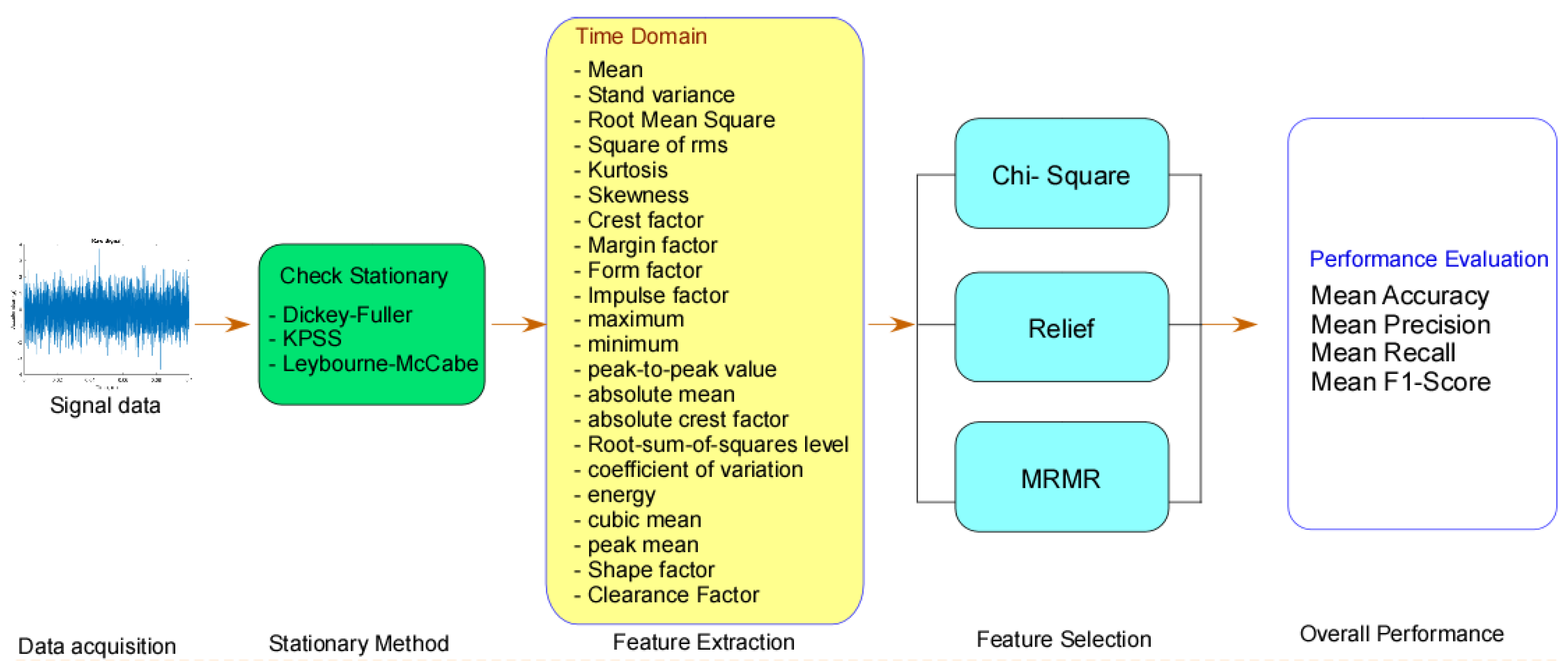
Figure 1.
Framework of Feature selection based on time domain.
Figure 1.
Framework of Feature selection based on time domain.
Laplacian Score is capable of characterizing the damage modes in each stage of loading, and the final failure is determined using this method (Barile et al., 2022).
3. CASE STUDY AND DATASET
3.1. Dataset
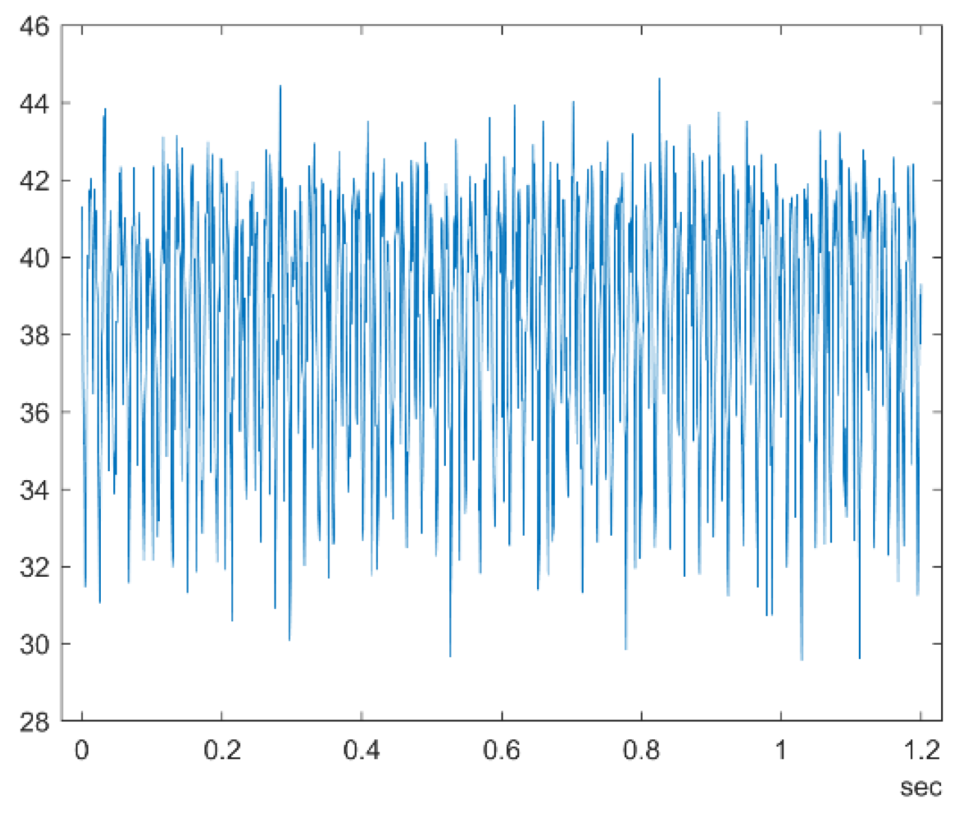
The dataset that was used in this research comes from the Simulink PumpSensor Dataset. This dataset contains 240 cells. As shown in
Figure 2, each cell contains 1200 rows with a time duration of 1.2 seconds. The pump motor speed is 950 rpm, or similar to 15.833 Hz. An eight-fault code is used to control signal flow and pressure.
3.2. Framework
The proposed method's framework, which is split into four steps (stationary check, time domain feature extraction, feature selection, and performance evaluation), is shown in
Figure 1.
3.3. Feature Extraction
In this research, we use two main feature extraction : time domain dan frequency domain. Time domain : Mean (Malikhah et al., 2021) ,Stand variance, Root Mean Square (Boonyakitanont et al., 2020) ,Square of rms, Kurtosis, Skewness, Crest factor, Margin factor, Form factor, Impulse factor, maximum, minimum, peak-to-peak value, absolute mean, absolute crest factor, Root-sum-of-squares level, coefficient of variation, energy, cubic mean, peak mean, Shape factor, Clearance Factor (Liu et al., 2021) . Several time domain can be describes as equation 1 – 8 :
where x(i) : signal input for i-th lines (i = 1,...,N, N is the number of accelerometer signals).
3.4. Performance Evaluation
Performance evaluation based on the confusion matrix : True Positif (TP), False Negative (FN), False Positive (FP), True Negative (TN) as shown in eq. 21. Four evalution criteria : Accuracy, Precision, Recall and F1 Score were used to examine the accuracy of the pump sensor fault classification. The following are the formulas for those evaluations (Singh et al., 2022) :
4. RESULT AND DISCUSSION
The study results from the framework were explained in this section.
4.1. Result
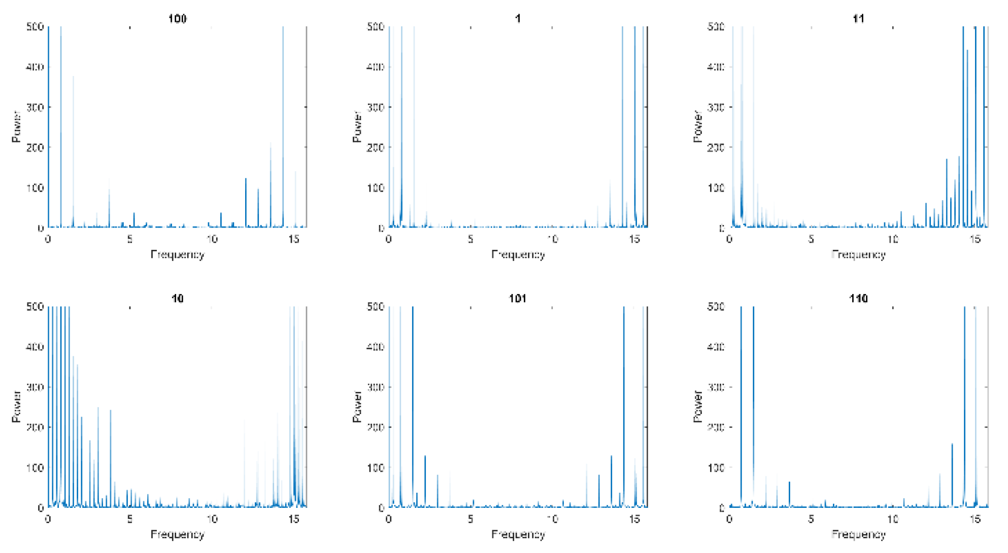
Multiple time domain and frequency domain feature extractions were used to extract the signal flow. As shown in
Figure 3, the frequency domain was used to extract the 8 fault codes (equal to 0, 1, 10, 11, 100, 101, 110, and 111). It is clear that each fault has different characteristics. The sum of the highest frequencies was held at fault 11 code (in high frequencies) and fault 10 code (in low frequencies).
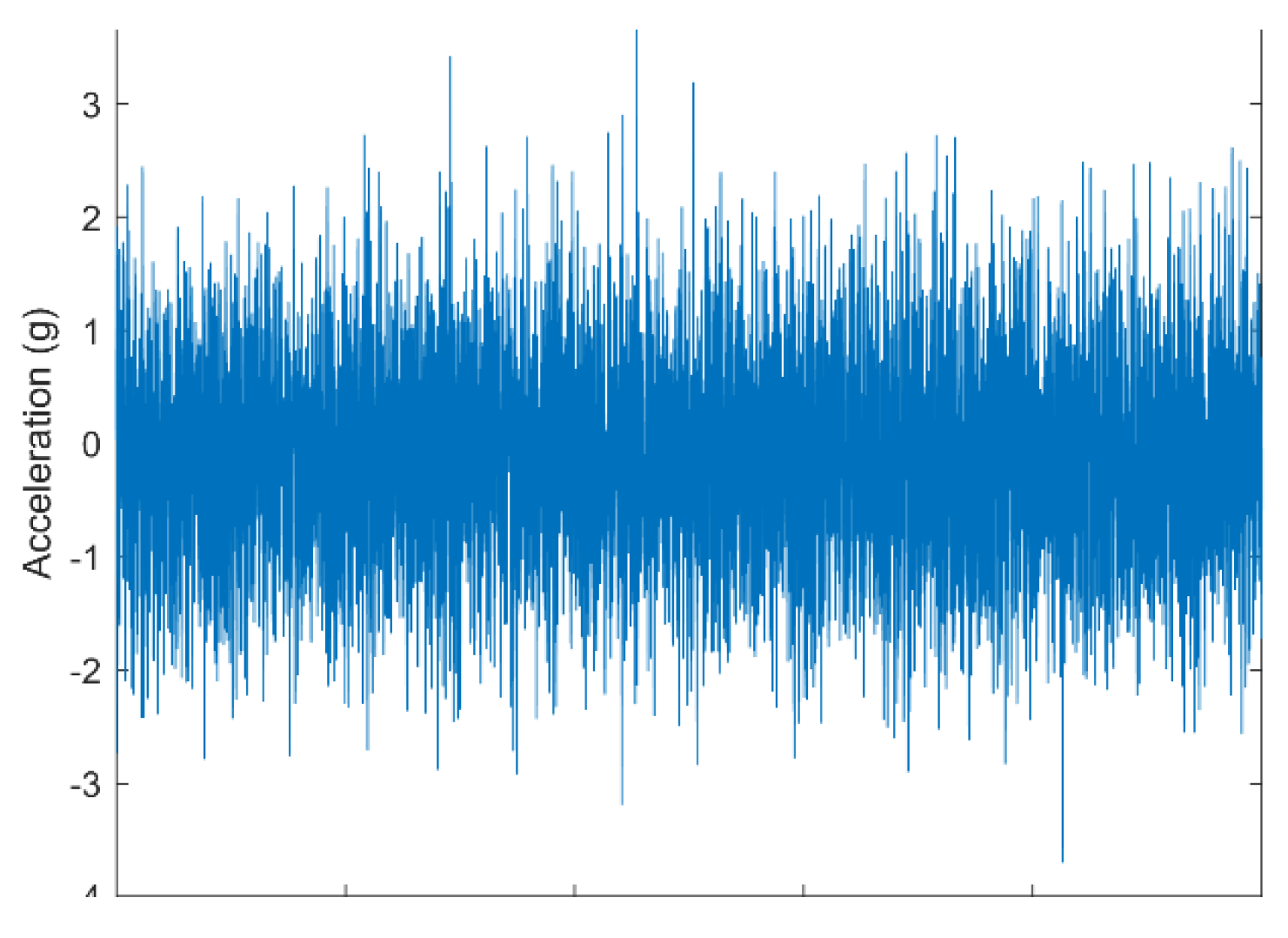
Using table 1, only Kwiatkowski–Phillips–Schmidt–Shin (KPPS) gives information that the dataset was stationary. This mean that the signal were not change over mean and variance over times. For Augmented Dickey–Fuller (ADF) test, we found that the pValue > 0.05, that means that hypothesis equal to zero is rejected, we then conclude that the model is stationary. Different with others, Leybourne-McCabe (LMC) demonstrates the non-stationarity of a signal. On the basis of this and picture 4, we can assume that the signal was Stationary.
After determining that the signal was stationary, the retrieved signal can perform time-domain feature extraction. Extracted from the time domain are 22 features. Using Chi-Square, Relief, and Minimum Redundancy Maximum Relevance, the data was then utilized to determine the most advantageous characteristic (MRMR). The results of the three approaches are presented in
Table 2 and
Table 3.
The best chi-square was the one with time domain numbers 9 and 15 according to
Table 2. There are the maximum and Root Mean Square values of the time domain signal. Based on
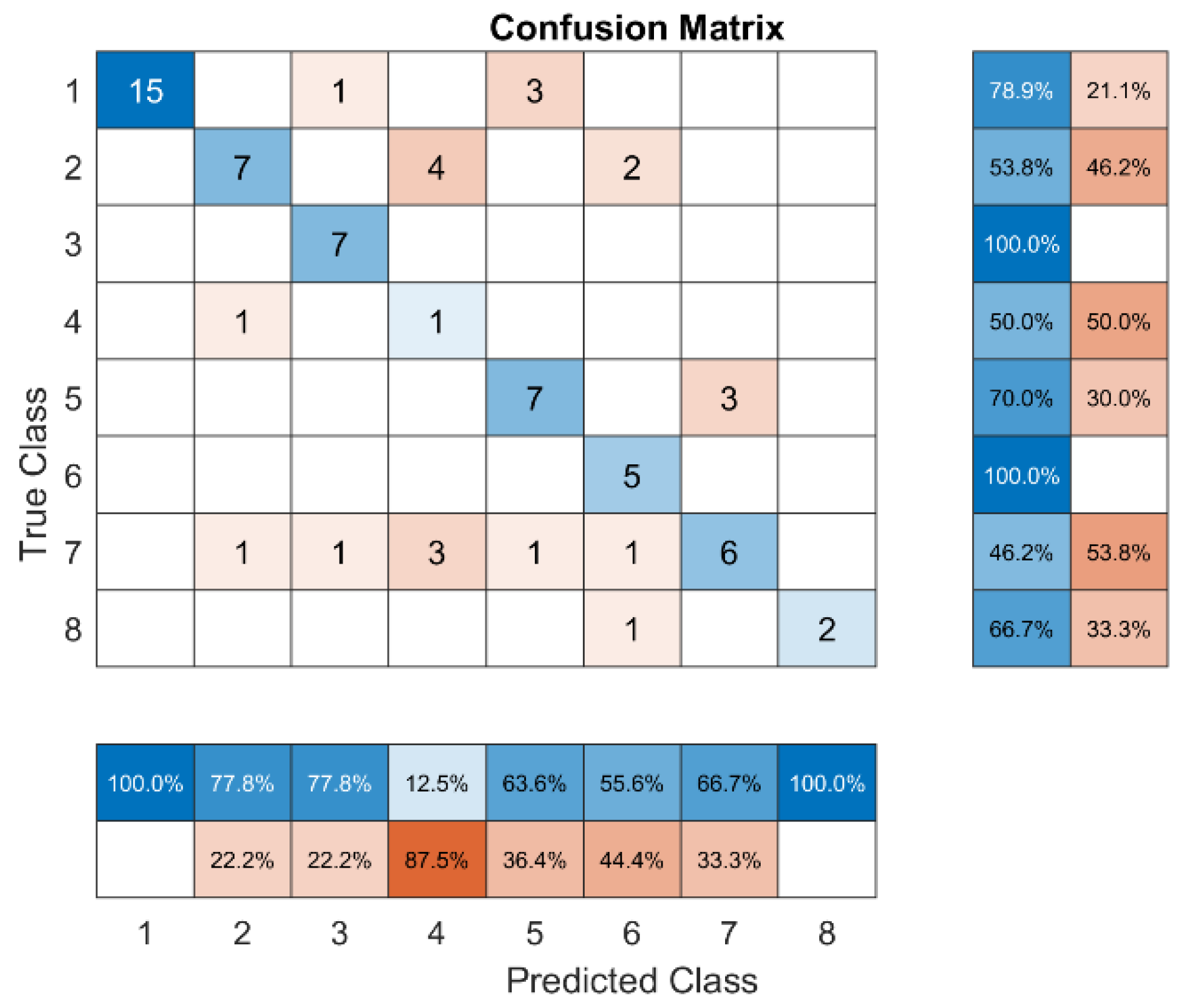
Figure 4, classes 1 and 8 had the most accurate fault code predictions, at 100%. Class 4 had the least accurate fault code predictions, at about 12.5%. With a total score of 69.44%, the chi-square feature selection was able to figure out the class.
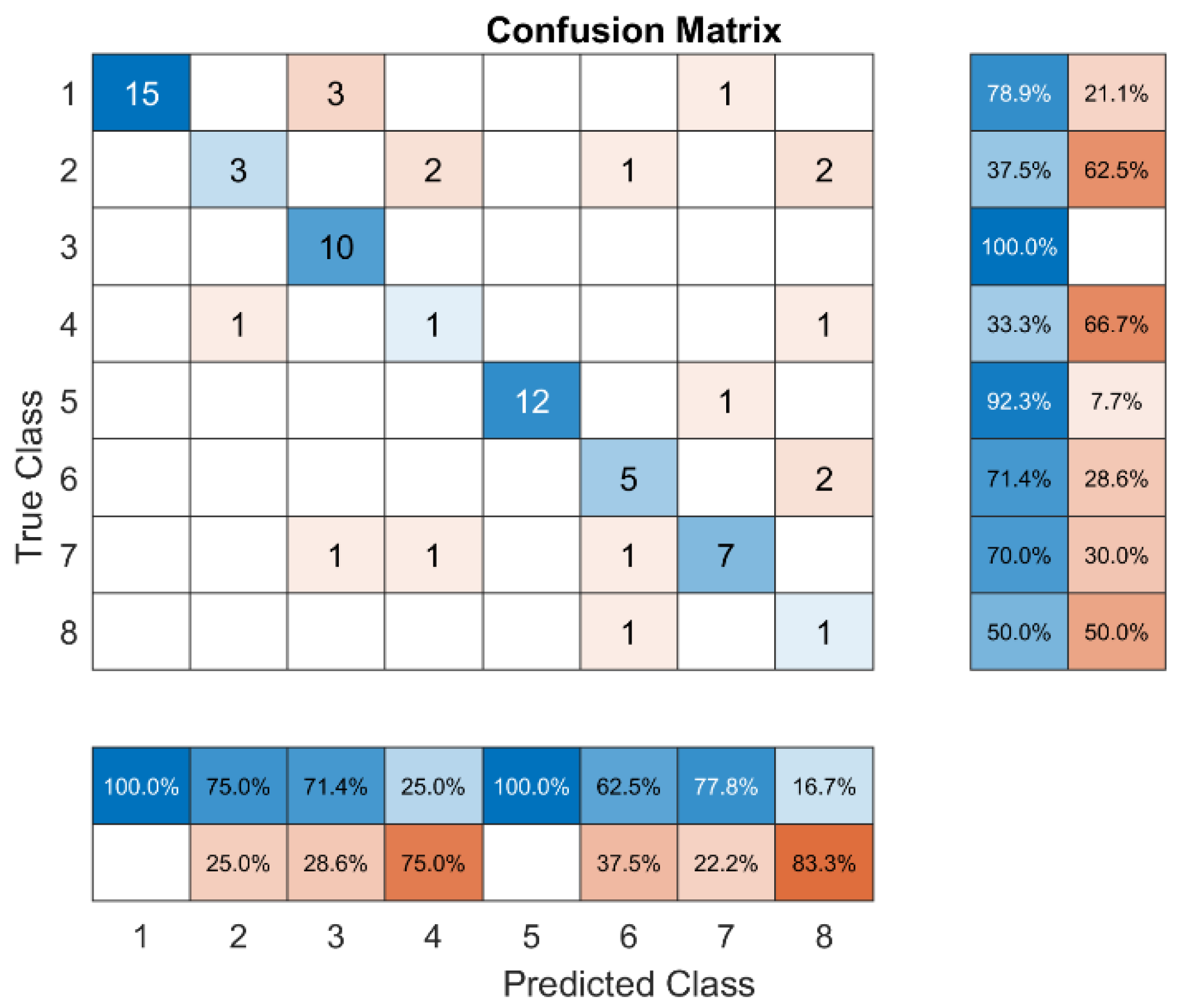
Figure 5 shows that in Class 1, accuracy is 94.4 percent for both recall and precision, and F1 scores are 79, 100, and 88 percent, respectively. The most accurate class was 5 (92%), and the least accurate class was 4 (33%). The class 8 had the least accurate recall (94.4% for both recall and precision) and the lowest F1 score (79, 100, and 88%). The most accurate class was 5 (92%), and the least accurate class was 4 (33%). The class 8 had the least amount of recall, at 17%, and the class 1 had the most, at 100%. So, the lowest F1 score was in class 8, and the highest was in class 5.
Overall, MRMR does not provide accurate, precise, recall, or F1 scores in all classes.
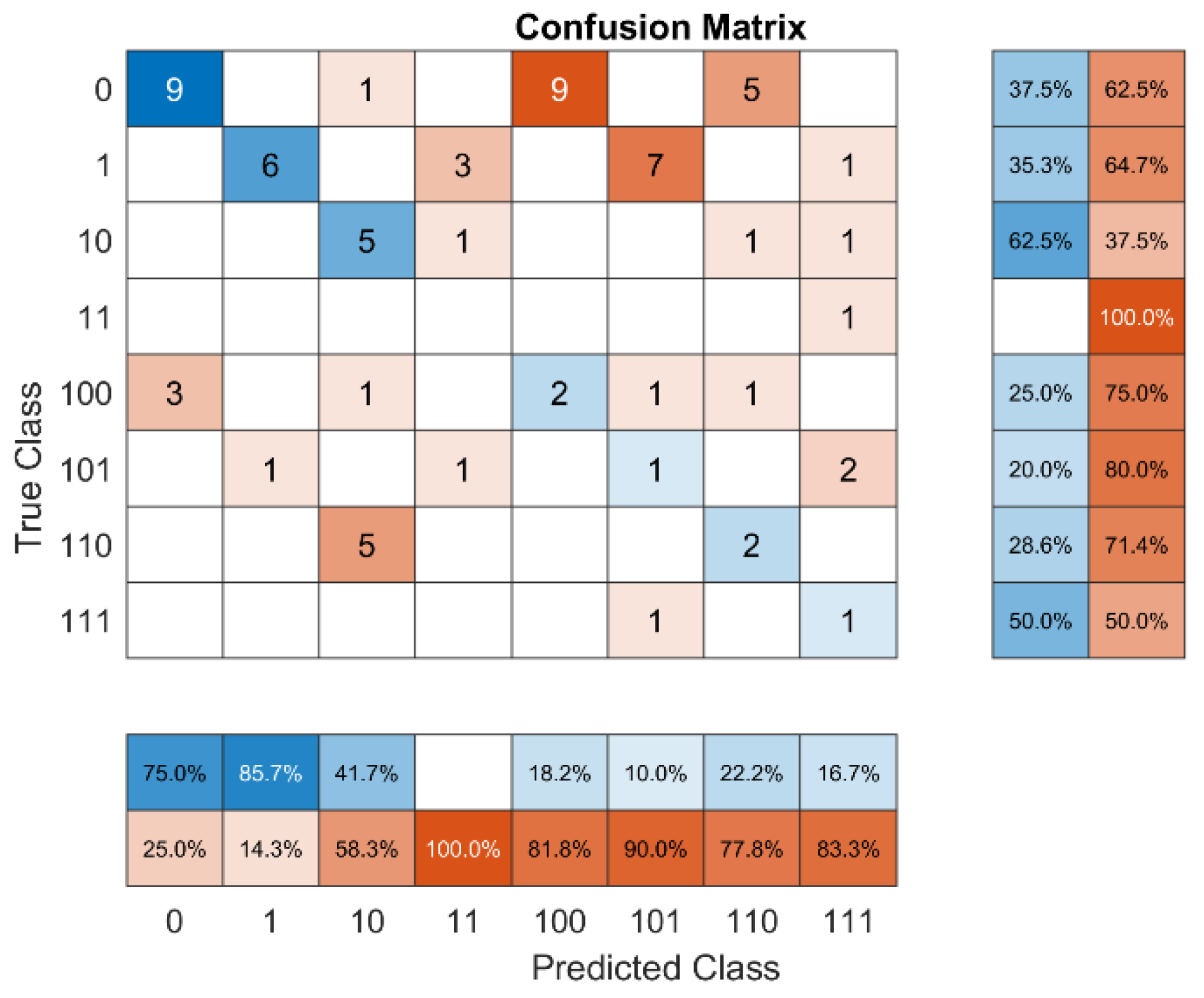
Figure 6 shows that class 4 had the lowest precision, recall, and F1 scores with values of 0 percent, respectively. Furthermore, in all classes, the average level of accuracy is 25%. Of all the ways to choose features, Class 8 has the worst recall. Class 1 only gets a recall score of 38% from MRMR, and class 5 only gets an F1 score of 25%. This isn't as good as other methods.
4.2. Comparison Result
To assess the performance of the various feature selection approaches outlined in
Section 4.1, we use equations 10–14 to calculate accuracy, precision, sensitivity, recall, and F1 score. ADF and KPSS indicate that the signal is stationary, as determined by the stationary check. We employ a time-domain stationary signal to extract the accelerometer based on this. Only two feature selections accurately depict the total performance. In contrast, each error code class can detect precision and accuracy.
Table 1.
Comparison of Stationary Method based on Signal Pump Sensor.
Table 1.
Comparison of Stationary Method based on Signal Pump Sensor.
| Method |
Hypothesis |
pValue |
Stats value |
cValue |
Status |
| ADF |
0 |
0,224610399 |
-1,166537974 |
-1,9416 |
Stationary |
| KPSS |
0 |
0,1 |
0,009554372 |
0,146 |
Stationary |
| LMC |
1 |
0,01 |
0,317521293 |
0,146 |
Non-stationary |
Table 2.
Feature selection ranking method based on 25 time-domain feature extraction.
Table 2.
Feature selection ranking method based on 25 time-domain feature extraction.
| Method |
Rank 1 |
Rank 2 |
Rank 3 |
Rank 4 |
Rank 5 |
| Chi-Square |
9 |
15 |
21 |
22 |
19 |
| Relief |
19 |
21 |
22 |
15 |
25 |
| MRMR |
17 |
23 |
16 |
24 |
2 |
| Laplacian |
21 |
6 |
9 |
1 |
20 |
Table 3.
Comparison of Performance Matrix between Chi-Square, Relief, MRMR and Laplacian.
Table 3.
Comparison of Performance Matrix between Chi-Square, Relief, MRMR and Laplacian.
| Method |
Overall Accuracy |
Overall Precision |
Overall Recall |
Overall F1 Score |
| Chi-Square |
0.6944 |
0.7070 |
0.6924 |
0.6996 |
| Relief |
0.75 |
0.6669 |
0.6605 |
0.6637 |
| MRMR |
0.5139 |
0.5784 |
0.4924 |
0.5320 |
| Laplacian |
0.5972 |
0.6139 |
0.5355 |
0.5720 |
5. CONCLUSION
In this paper, we presented a framework based on a formulation of a recently proposed model to work in prognostic health management. We applied it in pumpsensor dataset which is the signal is stationary based on the ADF and KPSS method. Moreover, 22 time domain feature for stationary dataset were used for extract the signal from accelerometer amplitude. The 22 feature then select using four feauture selection methods. The Chi-square method give overall high precision, recall and F1 score while in contrast the Relief method give overall high accuracy. Furthermore, the results have shown that this framework is capable to use for signal processing in stationary dataset for selecting best ranking feature.
References
- Bahassine, S., Madani, A., Al-Sarem, M., & Kissi, M. (2020). Feature selection using an improved Chi-square for Arabic text classification. Journal of King Saud University - Computer and Information Sciences, 32(2), 225–231. [CrossRef]
- Barile, C., Casavola, C., Pappalettera, G., & Paramsamy Kannan, V. (2022). Laplacian score and K-means data clustering for damage characterization of adhesively bonded CFRP composites by means of acoustic emission technique. Applied Acoustics, 185, 108425. [CrossRef]
- Ben Amor, L., Lahyani, I., & Jmaiel, M. (2018). Data accuracy aware mobile healthcare applications. Computers in Industry, 97, 54–66. [CrossRef]
- Biswas, A. R., & Giaffreda, R. (2014). IoT and cloud convergence: Opportunities and challenges. 2014 IEEE World Forum on Internet of Things, WF-IoT 2014, 375–376. [CrossRef]
- Boonyakitanont, P., Lek-uthai, A., Chomtho, K., & Songsiri, J. (2020). A review of feature extraction and performance evaluation in epileptic seizure detection using EEG. Biomedical Signal Processing and Control, 57, 101702. [CrossRef]
- Buchaiah, S., & Shakya, P. (2022). Bearing fault diagnosis and prognosis using data fusion based feature extraction and feature selection. Measurement: Journal of the International Measurement Confederation, 188(November 2021), 110506. [CrossRef]
- Chen, H., Wang, Z., & An, Y. (2022). Pollen Recognition and Classification Method Based on Local Binary Pattern. Lecture Notes of the Institute for Computer Sciences, Social-Informatics and Telecommunications Engineering, LNICST, 424 LNICST, 532–539. [CrossRef]
- Davidson, I., & Tayi, G. (2009). Data preparation using data quality matrices for classification mining. European Journal of Operational Research, 197(2), 764–772. [CrossRef]
- Ghosh, P., Azam, S., Jonkman, M., Karim, A., Shamrat, F. M. J. M., Ignatious, E., Shultana, S., Beeravolu, A. R., & De Boer, F. (2021). Efficient prediction of cardiovascular disease using machine learning algorithms with relief and lasso feature selection techniques. IEEE Access, 9, 19304–19326. [CrossRef]
- Katona, A., & Panfilov, P. (2018). Building predictive maintenance framework for smart environment application systems. Annals of DAAAM and Proceedings of the International DAAAM Symposium, 29(1), 0460–0470. [CrossRef]
- Kothamasu, R., Huang, S. H., & Verduin, W. H. (2006). System health monitoring and prognostics - A review of current paradigms and practices. International Journal of Advanced Manufacturing Technology, 28(9), 1012–1024. [CrossRef]
- Li, S., Ren, S., & Wang, X. (2013). HVAC Room temperature prediction control based on neural network model. Proceedings - 2013 5th Conference on Measuring Technology and Mechatronics Automation, ICMTMA 2013, 606–609. [CrossRef]
- Liu, Y., Hu, Z., & Zhang, Y. (2021). Bearing feature extraction using multi-structure locally linear embedding. Neurocomputing, 428, 280–290. [CrossRef]
- Majeed, M. T., Ozturk, I., Samreen, I., & Luni, T. (2022). Evaluating the asymmetric effects of nuclear energy on carbon emissions in Pakistan. Nuclear Engineering and Technology, 54(5), 1664–1673. [CrossRef]
- Malikhah, M., Sarno, R., & Sabilla, S. I. (2021). Ensemble Learning for Optimizing Classification of Pork Adulteration in Beef Based on Electronic Nose Dataset. International Journal of Intelligent Engineering and Systems, 14(4), 44–55. [CrossRef]
- Parhizkar, T., Aramoun, F., Esbati, S., & Saboohi, Y. (2019). Efficient performance monitoring of building central heating system using Bayesian Network method. Journal of Building Engineering, 26(January), 100835. [CrossRef]
- Parssian, A., Sarkar, S., & Jacob, V. S. (2004). Assessing data quality for information products: Impact of selection, projection, and cartesian product. Management Science, 50(7), 967–982. [CrossRef]
- Rahman, M. M., & Alam, K. (2021). Clean energy, population density, urbanization and environmental pollution nexus: Evidence from Bangladesh. Renewable Energy, 172, 1063–1072. [CrossRef]
- Reinhardt, A., Englert, F., & Christin, D. (2015). Averting the privacy risks of smart metering by local data preprocessing. Pervasive and Mobile Computing, 16(PA), 171–183. [CrossRef]
- Singh, V., Mathur, J., & Bhatia, A. (2022). A Comprehensive Review: Fault Detection, Diagnostics, Prognostics, and Fault Modelling in HVAC Systems. International Journal of Refrigeration. [CrossRef]
- Sumaiya Thaseen, I., & Aswani Kumar, C. (2017). Intrusion detection model using fusion of chi-square feature selection and multi class SVM. Journal of King Saud University - Computer and Information Sciences, 29(4), 462–472. [CrossRef]
- Wollschalaeger, M. (2017). The Future of Industrial Communication. Industrial and Engineering Chemistry, 12(4), 370–376. [CrossRef]
|
Disclaimer/Publisher’s Note: The statements, opinions and data contained in all publications are solely those of the individual author(s) and contributor(s) and not of MDPI and/or the editor(s). MDPI and/or the editor(s) disclaim responsibility for any injury to people or property resulting from any ideas, methods, instructions or products referred to in the content. |
© 2023 by the authors. Licensee MDPI, Basel, Switzerland. This article is an open access article distributed under the terms and conditions of the Creative Commons Attribution (CC BY) license (http://creativecommons.org/licenses/by/4.0/).
