1. Introduction
Individuals of many species disperse from one habitat patch to the another for a variety of reasons, including ecological factors and human disturbances (Fourcade, 2016). For a few species, dispersion outside of their native area is a regular occurrence and a required part of their life cycle (Clobert et al., 2009, Montero-Pau and Serra, 2011). Several landscape characteristics in every focal landscape complex might inhibit or facilitate such dispersals (Shanu et al., 2019). To study these dispersals, the possibility of dispersion, and dispersal patterns of individuals of distinct species, it is critical to understand the interaction of the species with the underlying landscape features (Carter et al., 2015).
The dispersal of species occurs naturally, as aforementioned. In order to avoid inbreeding, control food chain pressure, and maintain other ecologically significant features of each focal landscape, species disperse from one home range to the next (Bulte and Damania, 2008). Therefore, a vital aspect of nature that is necessary to maintain equilibrium among various phenomena and, consequently, to maintain the ecological balance is species dispersal (Holloway and Miller, 2017). It might take place in a single Protected Area (PA) or across several PAs. Because both of these dispersals are essentially the same, they have a shared origin. Any focal landscape may experience a variety of kinds of collaboration, defections, support, and multilayer conflicts, all of which can facilitate or obstruct species dispersal (Egyed and Grunbacher, 2004).
Landscape complexes have a variety of biotic and abiotic traits and are dynamic. These traits come together to form a group of elements that interact with the dispersing species and provide it with support on either a favorable or negative scale (ØRsted et al., 2017). Therefore, a specie's individual dispersion is an emergent phenomenon resulting from the interactions of the landscape complex. Additionally, each parameter interacts with different species in different ways, and each species receives a distinct level of support or inhibition. Hence, it may be claimed that a species' movement and mobility patterns within a landscape are unique to that species (Chassagneux et al., 2019). For instance, the mobility of an elephant (Elephas maximus) might not be supported by the presence of a large chital (Axis axis) population in any landscape grid, however the dispersion of a tiger (Panthera tigris tigris) might. The discussion above explains how each species interacts with landscape factors differently, leading to species-specific movement patterns in any focal landscape.
Finding and analyzing the tiger's dispersal patterns in a hypothetical environment that has all essential components of any landscape is the aim of this study. The tiger is the focal species. Such a model would need to understand why an individual migrates outside of their natal range, which would be a vital objective (following the life event models of tiger). To accommodate the demands and wants of a dispersing tiger, the knowledge learned about the reason for migration may be employed (Damodaran, 2007). To understand more about the dispersing tiger's travel behaviour, these demands might potentially be reproduced.
One method to achieve the aforementioned objective is to initially divide the landscape into grids of equal size. As a consequence, each grid functions as an element of the landscape's matrix. The interactions in each grid are then simulated to produce a cost surface that is placed over the landscape matrix, resulting in scores for each grid that indicate whether it encourages or prevents tiger passage across it (Jones and Kaiser, 2005).
This paper's major goal is to present a fundamental computational framework for better understanding and forecasting tiger dispersal patterns in any setting. Every claim made in this study is supported by cognitive definitions of a dispersing tiger's needs and the presence or absence of particular landscape quality in every grid of the landscape matrix (Brady et al., 2009). As a result, every encounter is greatly influenced by the main landscape structure.
In this paper, the difficulty of understanding tiger dispersal patterns in a landscape is treated as a cost allocation problem. The reason why tigers leave their native habitat is then incorporated into the job via dispersion weights. A cognitive evaluation of tiger requirements based on dispersion causes determines the dispersion weights (Kacprzak, 2019). It provides the dispersion coefficient for each landscape characteristic, demonstrating how much each attribute impacts the grid's cost distribution. Additionally, we model the interaction of each attribute using a two-player prisoner's dilemma game, and the payoffs are merged with the dispersion coefficients to provide a starting cost to each grid (Cho, 2014). One of the most important and variable features of the environment that affects tiger dispersion is the presence or absence of co-predators in the grids (Reddy et al., 2012). Only a few hardbound scores are provided, and even the presence of co-predators is classified based on relative strengths in order to produce a secondary cost matrix on the landscape matrix. The original and secondary matrices are combined to provide the final cost matrix for the entire landscape complex.
The following arguments do not take into account any real-world information gathered by a GIS procedure and a typical field investigation. The findings might serve as a model for conservationists and wildlife managers to utilize when making judgments about tiger dispersal patterns since it focuses on the existence or absence of attributes in different grids in the complex and the ease of mobility.
The foundation for the work's materials and methods is laid out in succeeding section, and the hypothetical landscape that was used to construct and evaluate the mathematical model presented in this study is explained further. Finally, the study's methodology is detailed, and the remainder of the paper is devoted to the study's outcomes, analysis, and conclusion.
2. Matrices, Dispersal Weights and Game Theory
The current paper offers a model for realistic cost allocation for dispersing tigers in a complex terrain using a few particular areas of mathematics. The fundamental concepts of various subjects are discussed in this part to make the work self-contained.
Matrix: A matrix is a collection of rows and columns that each have the same amount of entries. The element arrangement of a matrix is represented formally as follows:
where the elements of the matrix
is denoted as
and the order of the matrix is
, which signifies that there are
m rows and
n columns in the matrix (Pfaffel and Schlemm, 2012). The landscape is structured as a matrix with grids as its elements.
Dispersal Weights: The term "dispersal weight" refers to a set theoretic technique to ordering the components of any given set based on their probability and needs (Gutman, 2021), as proposed in this work. For a given set
and a given set of parameters
for deciding the importance of each element in
A, the Dispersal weight
M is given as:
The importance of dispersal weights has been addressed since they will be used to rate landscape features based on the reason for tiger dispersion.
Game Theory: Game theory has been utilized to simulate the interaction (Webb 2007) between landscape characteristics and migratory tigers in this study. A game is defined as a three-tuple, where denotes the number of players, denotes the strategy set for each player, and ∏ denotes the associated payoff for each player, such that, where denotes the strategy chosen by player from the strategy set θ for a move. Thus, when one player plays a certain strategy against the other, the payoff is the score they receive (Shanu et al., 2019).
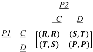
There are many different types of games that may be used to mimic interactions. In order to represent the binary interactions between the tigers and the landscape characteristics in this work, a two-person’s prisoner dilemma game has been used. The game is represented as:
where
, present two players of the game. Next,
represent the game's strategy set in which each player can either cooperate
(C) or defect
(D). In a strategic form, the payoff matrix expressed in the form of a set in the above representation is expressed as:

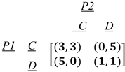
where, R represents the reward for mutual cooperation and has a numeric value of 3, S represents the sucker's payoff and has a numeric value of 0, T represents the reward for defect temptation and has a numeric value of 5, and P represents the punishment for mutual defection and has a numeric value of 1 (Hofbauer and Sigmund 1998; Webb 2007). As a result, the reward matrix may alternatively be represented numerically as:
The ideas in this work are based on the binary interaction between tigers and each grid's landscape characteristics. The two-person prisoner dilemma game was utilized to record these exchanges (Shanu & Bhattacharya, 2018).
3. Hypothetical Landscape for the Study
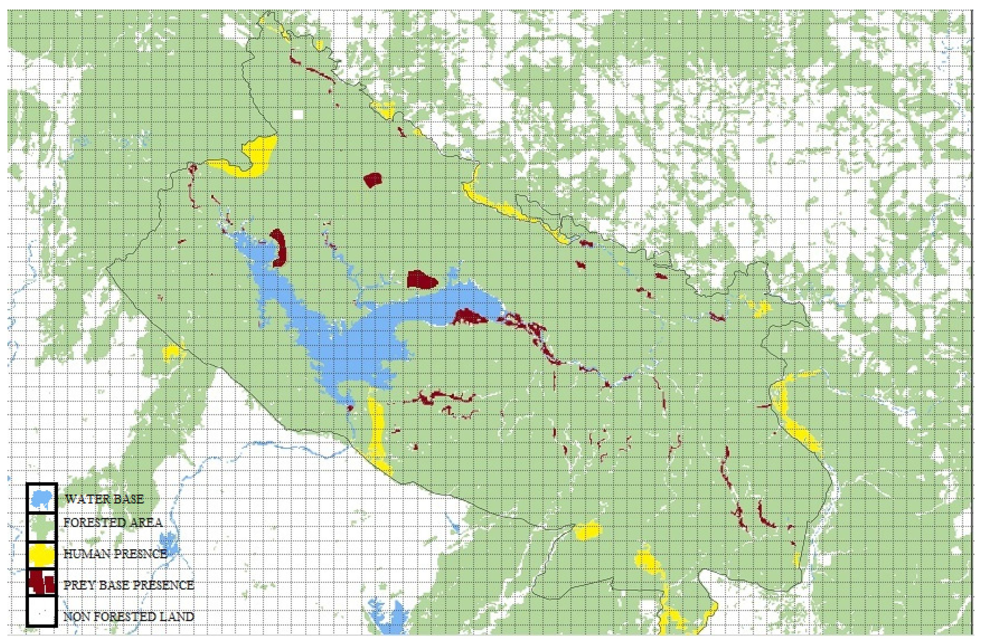
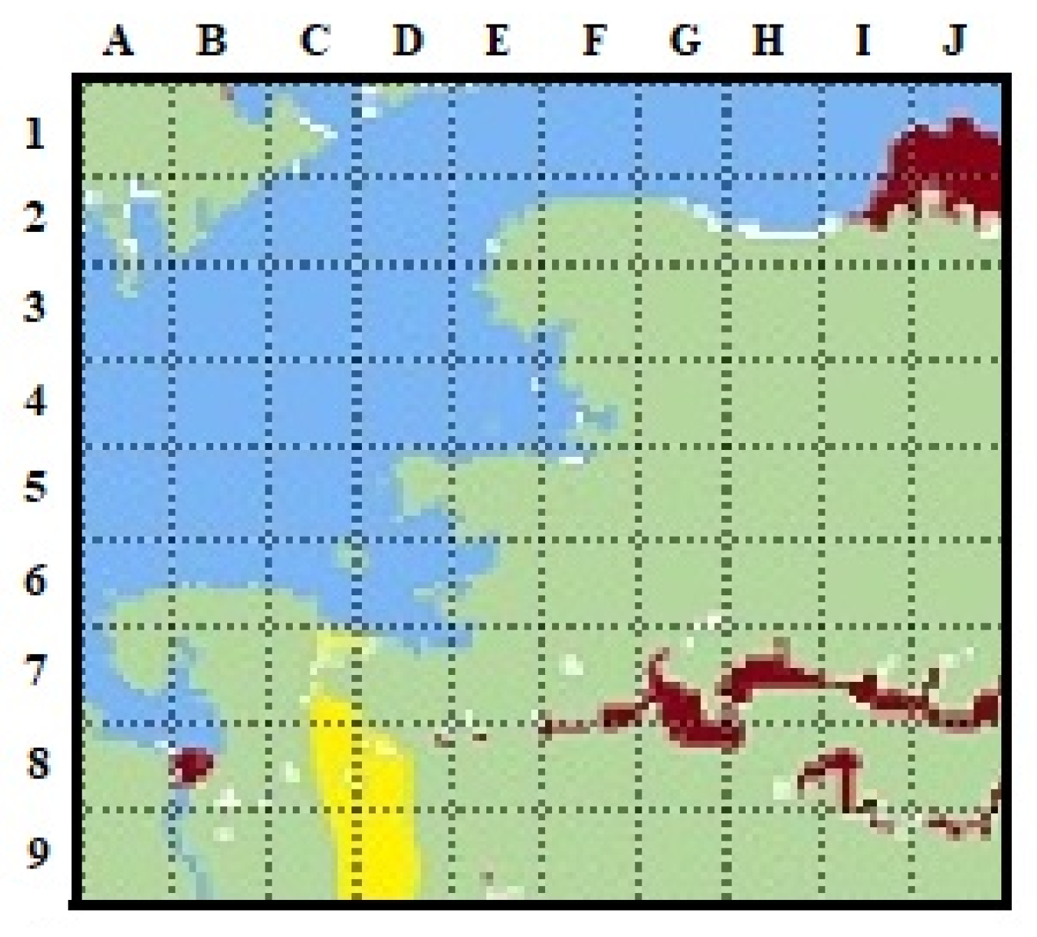
The hypothetical landscape that was used in this work for modelling purposes is shown in
Figure 1. The presence of humans, animals as prey, non-forested terrain, and water bodies are all crucial landscape aspects to take into account (Trisurat, 2010). Only a few crucial aspects are looked at with the aim of presenting the model and related mathematical framework. There are many more biotic and abiotic elements that will be present in the landscape and all of these parameters must be considered while working on the tiger dispersal pattern.
The forest region mentioned here includes dense, moderately dense, open, and meadow-like woodlands. The presence of people symbolizes the land used for farming, animal grazing, and village settlements. All preferred species as well as injured species that the tigers could devour are included in the prey base. The non-forested terrain includes wasteland, which is devoid of vegetation. The final assessed water base parameters cover all sources of water, from naturally flowing rivers to department-built waterholes (Jhala et al., 2011). The landscape matrix is divided into important pixels using a grid for evaluation and afterwards observation of the landscape features. The model is created to take into consideration the presence or absence of dominating tigers over dispersing tigers, and each pixel of the landscape matrix is considered as a tiger habitat and territory in the hypothetical environment. As a consequence, each grid's collection of parameters is shown as:
where, WB represents water base, FA represents forested area, HP represents human presence, PB represents presence of a prey base and NF represents non-forested land.
4. Methodology
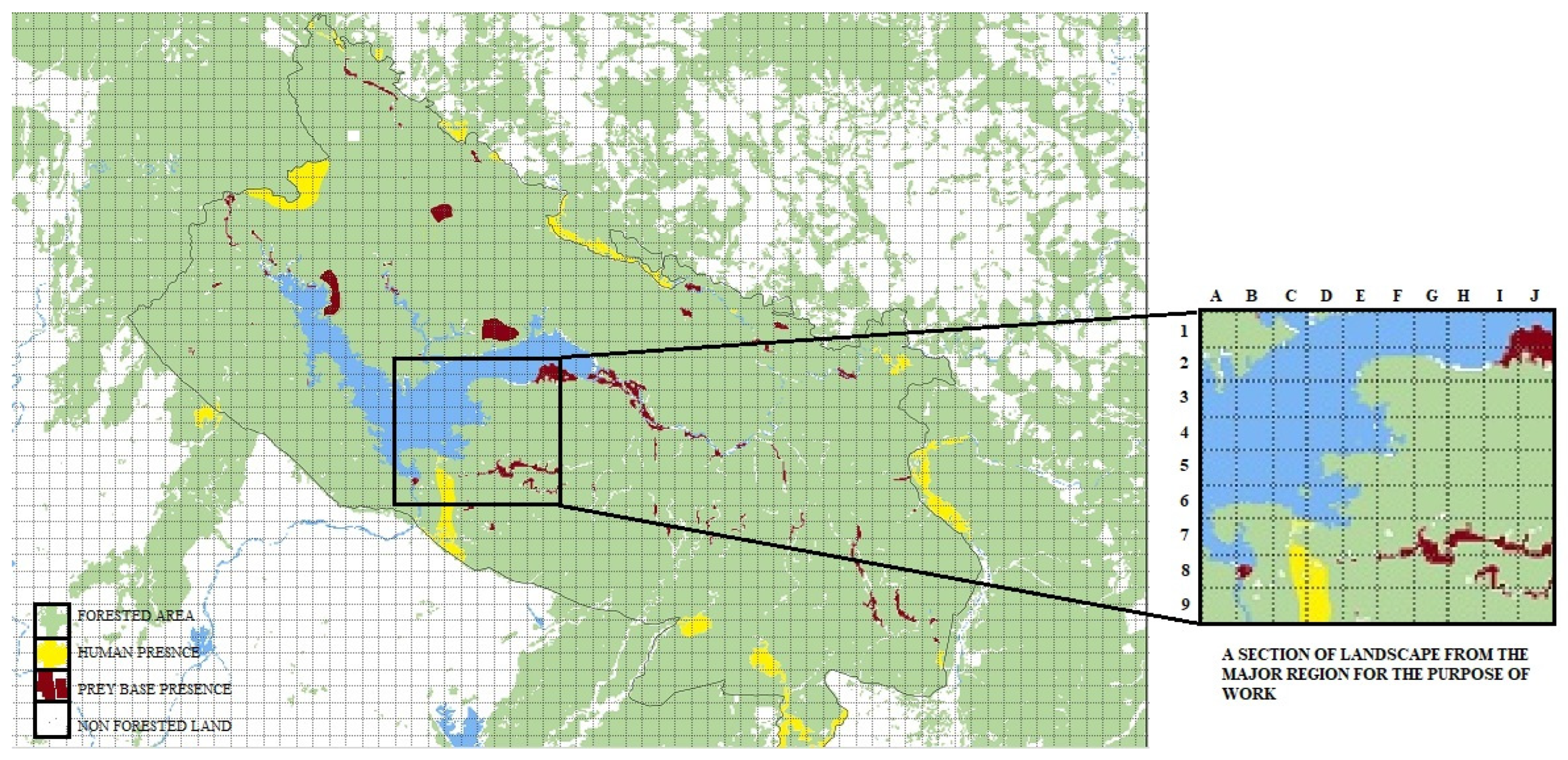
To demonstrate the model suggested in this work, a portion of the landscape matrix containing all the characteristics given in the Hypothetical Landscape section is studied with the border indicated in
Figure 2.
In order to comprehend tiger dispersal patterns better, the work aims to create a cost matrix that can be dispersed across the landscape. It should be noted that the cost matrix would depend on the source and sink aspects of the landscape (Etherington, 2016). When we discuss the source, we are referring to the elements from which a member of a species starts to disperse, whilst the other elements serve as sinks. For instance, the sink grids may be expressed as follows if F3 is the source grid in
Figure 2:
The preceding explanation clearly indicates that the costs of dispersion for every element of
S must be assessed. All of the discussed criteria are required during these evaluations, and one of the most important aspects is the presence or absence of other predators (Presser and Luoma, 2013). The existence of co-predators in the region and surroundings is a crucial factor in the tiger dispersion (Jhala et al., 2008).
Table 1 shows an assumption for the landscape section selected, with
indicating the presence of stronger co-predators or individuals, -1 indicating the presence of weaker individuals, and 0 indicating the absence of any individual.
Initially, the cause for an individual's dispersion is an essential factor in determining their dispersal pattern. Four critical life events from the tiger life cycle that influence the tiger dispersal pattern are examined for the sake of modelling. These occurrences are extremely beneficial because they allow to better grasp the physical and cognitive requirements of the dispersing individual (Ramesh et al., 2009). While modelling the dispersal situation and understanding the dispersal patterns, it also alters, the costs associated with each grid. These events, the reasons for dispersion, have been encoded in a manner, which are described in
Table 2 and are quite valuable for modelling.
Given the ramifications of the preceding, the cost of each grid is computed utilizing the landscape complex characteristics contained in the grid, the cause for dispersion and the presence/absence of co-predators. In this work, the cost is determined by three factors and given below as:
where α indicates the dispersion coefficient based on the cause for tigers' dispersion.
represents the payoff received by modelling a 2-Person’s prisoner dilemma game between the dispersing tiger and each parameter of set
G present in the grid
, given the reason for dispersion
and
represent the score received due to presence, absence as well as the dominance of co-predators in the grid.
For a more in-depth knowledge of the cost evaluations discussed above, the entire landscape may be seen as a network, with each grid acting as a vertex and the connections between the grid’s 8-neighborhoods acting as edges (Tabassum et al., 2018). Preferential movement in the proposed research work determines the beneficial links for tiger dispersion. The parameters of the grid or the components of
G depending on the cause for dispersion using the dispersion weights are ranked over the network as shown in
Table 3.
This is used to calculate the dispersion coefficient α. Membership value or the dispersion coefficient has been obtained based on the rank of the parameters according to their needs as:
Range of α lies between 0 and 1. Earlier studies of the recent past have been utilized to get the values of α, based on various reasons for dispersion (Shanu et al., 2019). The values of α obtained on the application of dispersion weights are shown in
Table 4.
After determining the degree of influence each element may have on the grid's cost, the interactions in the landscape are simulated using game theory (Turner, 1989). The interaction of migrating tiger with the landscape factors is a key focus of this work. As a result, we represent the problem in this work using the dispersing individual as one of the players in a two-person prisoner's dilemma game, with the landscape characteristics as the other players (Shanu et al., 2019). Therefore, the game's payoffs are obtained as:
Each of the factors in set
G either encourages or hinders tiger mobility in the landscape complex.
Table 5 illustrates the contribution of each parameter to any grid's cost, as well as the degree of support for migration of an individual through the grid.
As aforementioned, the presence or absence of co-predators is one of the most significant factors in determining tiger dispersion; the work aims to quantify the impact of this on the cost of a grid. Because interactions with co-predators can take many forms and applying game theory to describe the interaction of a dispersing tiger with co-predators may be problematic. Further, while these interactions may yield a benefit, they may also have negative consequences such as injuries, weakening, and other conflict-related losses, all of which can limit individual's mobility. With this in focus, the study assigns a high inhibitory discrete value of -10 to interactions with greater predators and a low supporting score of +3 to interactions with weaker predators. The score has been set at 0 for regions with no co-predators.
5. Results & Discussion
The suggested methodology has been used to conduct a thorough investigation of landscape characteristics for the computation of grid costs over a landscape complex in order to better understand the tiger dispersions (Yumnam et al., 2014). The cost allocation is done using the part of the hypothetical landscape depicted in
Figure 3 and the example with F3 as source. The tables below illustrate the presence and absence of parameters in the landscape matrix grids. In each table, 0 indicates the absence of the parameter whereas 1 indicates its presence.
Table 6.
Presence/Absence of Water Body.
Table 6.
Presence/Absence of Water Body.
| Code |
A |
B |
C |
D |
E |
F |
G |
H |
I |
J |
| 1 |
0 |
1 |
1 |
1 |
1 |
1 |
1 |
1 |
1 |
1 |
| 2 |
1 |
1 |
1 |
1 |
1 |
1 |
1 |
1 |
1 |
0 |
| 3 |
1 |
1 |
1 |
1 |
1 |
1 |
0 |
0 |
0 |
0 |
| 4 |
1 |
1 |
1 |
1 |
1 |
1 |
0 |
0 |
0 |
0 |
| 5 |
1 |
1 |
1 |
1 |
0 |
0 |
0 |
0 |
0 |
0 |
| 6 |
1 |
1 |
1 |
1 |
1 |
0 |
0 |
0 |
0 |
0 |
| 7 |
1 |
1 |
0 |
1 |
1 |
0 |
0 |
0 |
0 |
0 |
| 8 |
1 |
1 |
0 |
0 |
0 |
0 |
0 |
0 |
0 |
0 |
| 9 |
0 |
1 |
0 |
0 |
0 |
0 |
0 |
0 |
0 |
0 |
Table 7.
Presence/Absence of Forested Area.
Table 7.
Presence/Absence of Forested Area.
| Code |
A |
B |
C |
D |
E |
F |
G |
H |
I |
J |
| 1 |
1 |
1 |
1 |
0 |
0 |
0 |
0 |
0 |
0 |
0 |
| 2 |
1 |
1 |
0 |
0 |
1 |
1 |
1 |
1 |
1 |
1 |
| 3 |
0 |
0 |
0 |
0 |
1 |
1 |
1 |
1 |
1 |
1 |
| 4 |
0 |
0 |
0 |
0 |
0 |
1 |
1 |
1 |
1 |
1 |
| 5 |
0 |
0 |
0 |
1 |
1 |
1 |
1 |
1 |
1 |
1 |
| 6 |
1 |
1 |
1 |
0 |
1 |
1 |
1 |
1 |
1 |
1 |
| 7 |
1 |
1 |
1 |
1 |
1 |
1 |
1 |
1 |
1 |
1 |
| 8 |
1 |
1 |
1 |
1 |
1 |
1 |
1 |
1 |
1 |
1 |
| 9 |
1 |
1 |
1 |
1 |
1 |
1 |
1 |
1 |
1 |
1 |
Table 8.
Presence/Absence of Human Presence.
Table 8.
Presence/Absence of Human Presence.
| Code |
A |
B |
C |
D |
E |
F |
G |
H |
I |
J |
| 1 |
0 |
0 |
0 |
0 |
0 |
0 |
0 |
0 |
0 |
0 |
| 2 |
0 |
0 |
0 |
0 |
0 |
0 |
0 |
0 |
0 |
0 |
| 3 |
0 |
0 |
0 |
0 |
0 |
0 |
0 |
0 |
0 |
0 |
| 4 |
0 |
0 |
0 |
0 |
0 |
0 |
0 |
0 |
0 |
0 |
| 5 |
0 |
0 |
0 |
0 |
0 |
0 |
0 |
0 |
0 |
0 |
| 6 |
0 |
0 |
0 |
0 |
0 |
0 |
0 |
0 |
0 |
0 |
| 7 |
0 |
0 |
1 |
1 |
0 |
0 |
0 |
0 |
0 |
0 |
| 8 |
0 |
0 |
1 |
1 |
0 |
0 |
0 |
0 |
0 |
0 |
| 9 |
0 |
0 |
1 |
1 |
0 |
0 |
0 |
0 |
0 |
0 |
Table 9.
Presence/Absence of Prey Base.
Table 9.
Presence/Absence of Prey Base.
| Code |
A |
B |
C |
D |
E |
F |
G |
H |
I |
J |
| 1 |
0 |
0 |
0 |
0 |
0 |
0 |
0 |
0 |
1 |
1 |
| 2 |
0 |
0 |
0 |
0 |
0 |
0 |
0 |
0 |
1 |
1 |
| 3 |
0 |
0 |
0 |
0 |
0 |
0 |
0 |
0 |
0 |
0 |
| 4 |
0 |
0 |
0 |
0 |
0 |
0 |
0 |
0 |
0 |
0 |
| 5 |
0 |
0 |
0 |
0 |
0 |
0 |
0 |
0 |
0 |
0 |
| 6 |
0 |
0 |
0 |
0 |
0 |
0 |
0 |
0 |
0 |
0 |
| 7 |
0 |
0 |
0 |
0 |
0 |
1 |
1 |
1 |
1 |
1 |
| 8 |
0 |
1 |
0 |
0 |
0 |
1 |
1 |
1 |
1 |
1 |
| 9 |
0 |
0 |
0 |
0 |
0 |
0 |
0 |
0 |
1 |
1 |
Table 10.
Presence/Absence of Non-Forested Area.
Table 10.
Presence/Absence of Non-Forested Area.
| Code |
A |
B |
C |
D |
E |
F |
G |
H |
I |
J |
| 1 |
0 |
0 |
0 |
0 |
0 |
0 |
0 |
0 |
0 |
0 |
| 2 |
1 |
0 |
0 |
0 |
0 |
0 |
0 |
0 |
0 |
0 |
| 3 |
0 |
0 |
0 |
0 |
0 |
0 |
0 |
0 |
0 |
0 |
| 4 |
0 |
0 |
0 |
0 |
0 |
0 |
0 |
0 |
0 |
0 |
| 5 |
0 |
0 |
0 |
0 |
0 |
0 |
0 |
0 |
0 |
0 |
| 6 |
0 |
0 |
0 |
0 |
0 |
0 |
0 |
0 |
0 |
0 |
| 7 |
0 |
0 |
0 |
0 |
0 |
1 |
0 |
0 |
0 |
0 |
| 8 |
0 |
0 |
0 |
0 |
0 |
0 |
0 |
0 |
0 |
0 |
| 9 |
0 |
0 |
0 |
0 |
1 |
0 |
0 |
0 |
0 |
0 |
The scores are generated by modelling each interaction between a dispersing tiger and a landscape parameter after acquiring the presence and absence details of the parameters in the landscape matrix for all four distinct causes for migration (Epps et al., 2007), explained in
Table 2. The dispersion weight is calculated using the causes for dispersion, and the value of the dispersion coefficient reflects this as had been explained in
Table 4. In addition to the aforementioned factors, the costs of co-predator presence are taken into account. The final cost surface for all of the dispersion causes investigated in this study is computed and given in the form of a matrix in the
Table 11,
Table 12,
Table 13 and
Table 14.
The proposed work offers a fundamental mathematical framework for calculating the costs of a collection of landscape components that may help or hinder tiger’s dispersion from one location to another. The overall study's problem is to offer a computational model to extract the cost for landscape grids, modeling the cognitive knowledge and behaviour of tigers, using it to learn about tiger’s dispersion patterns (Rifaie et al., 2015). A significant result of this work is an in-depth investigation of the factors and how the tigers can use these factors for their mobility. The study also reveals important grids where tiger’s mobility may be tracked and observed as they leave their native region. This can be highly beneficial for wildlife stakeholders in terms of conservation and landscape design.
The work's main findings are given in the form of a matrix, which is represented by a series of tables:
Table 11,
Table 12,
Table 13 and
Table 14, which reveal several insights related to tiger dispersion. Finding the cost surface first uses the reason for the tiger's departure from its native area, which aids in the identification of the dispersing tiger's primary needs, and therefore the dispersal pattern. It also highlights the most important grids in the terrain where the tigers can disperse and settle, allowing more attention to the connecting pathways (Penjor et al., 2019; Minor and Urban, 2008).
The results demonstrate that there is a cost associated with each grid. The following is how the acquired costs in this work are linked to the tiger movement:
As a result, the higher the cost, the more likely the tiger is to disperse through the grid.
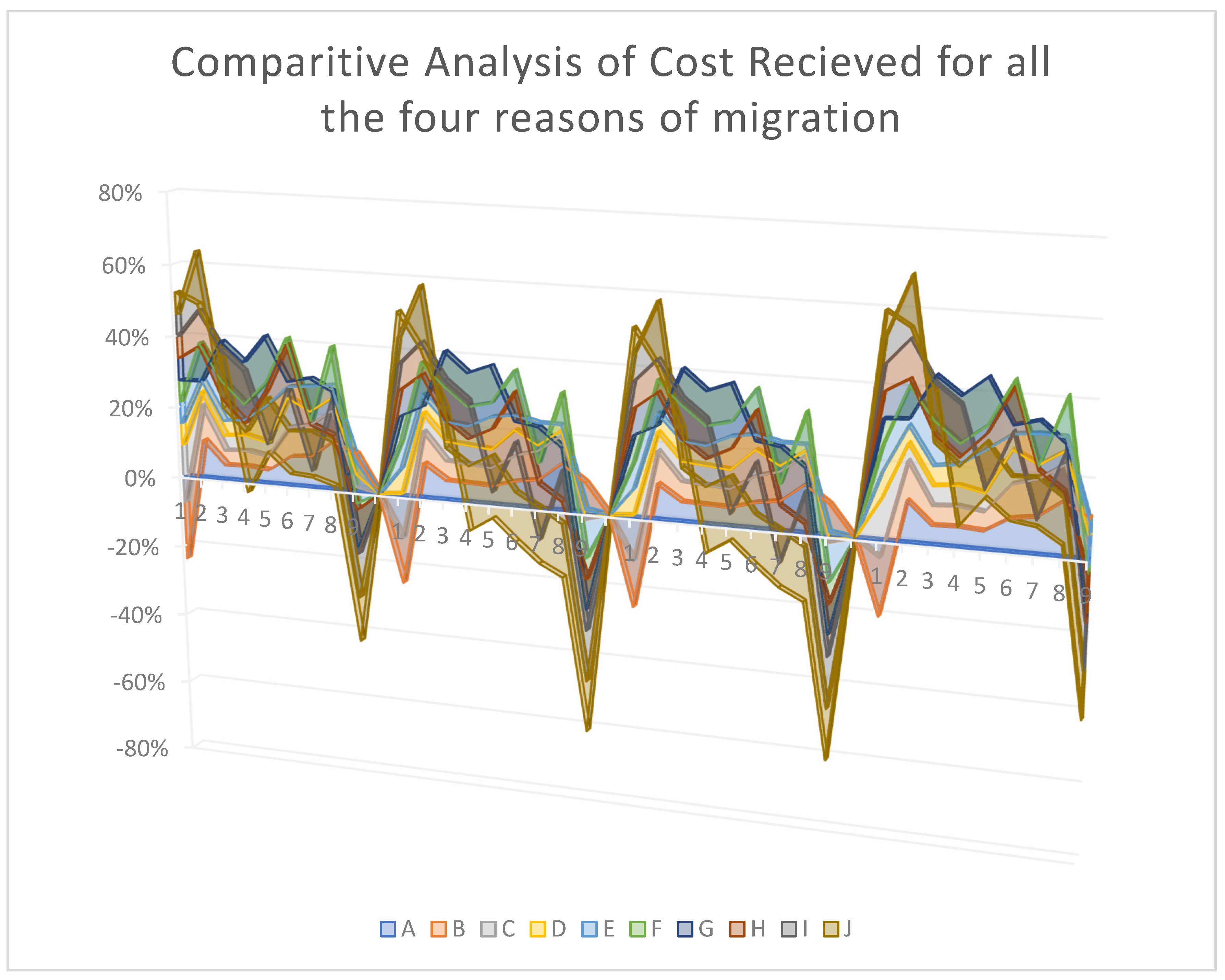
The cost and the tiger dispersion pattern owing to the expenses are examined after obtaining information on the tiger dispersion patterns utilizing the costs connected with the landscape complex (Sharma et al., 2013).
Figure 4 depicts the study and highlights a number of significant findings. First, it demonstrates that when tigers disperse out of their home area or for food, the costs are identical, and therefore the dispersion pattern is similar. Then, with minor modifications, it shows a link between the cost and the dispersion pattern of tigers dispersing for dominance or breeding. Furthermore, it is observed that tigers going out for dominance and breeding have more mobility choices than tigers travelling out for food or leaving their home zone. It also informs that tigers moving for food and outside of their native range are both inexperienced and younger than the other dispersing tigers, or they are elderly and defeated.
Species dispersal is a crucial aspect to comprehend in order to obtain understanding about a variety of conservation concepts (Meretsky et al., 2011). Wildlife corridor design, habitat suitability index, and other essential aspects are some of the key conservation concepts associated with species dispersal (Aziz and Rasidi, 2014; Perkl, 2016). The creation of a cost surface across the landscape complex aids not only in comprehending dispersal but also in determining dispersal patterns, which may then be used for conservation reasons (Horns and ŞEkercioğlu, 2018). Because of the preceding discussion, it is clear that a cost surface over a landscape matrix aids in the development of suitable conservation models.
Another insight provided by the suggested approach in this study is the ability to extract the sensitivity of a grid for tiger dispersal across it (Yumnam et al., 2014). It is clear which grids aid tiger dispersal and which grids obstruct tiger dispersal. As a result, the costs and vulnerability of a grid are related as follows:
Understanding a grid's vulnerability is critical because it depicts grids that may require human intervention in order to facilitate tiger dispersion and hence protect the species (Rathore et al., 2012). As a result, related vulnerabilities may be viewed as a guiding concept for developing ideal conservation measures.
Numerous analogies and comments made above imply the requirement of constructing the cost surface throughout a landscape matrix. All of the conversations point to the fact that finding a cost matrix and projecting it onto a surface helps to understand how different species disperse across a complex environment and how they do so, which in turn helps with conservation using different models.
6. Conclusions
The current study seeks to obtain a cost surface over the landscape complex, which displays the landscape complex as a matrix, and detect the tiger dispersal pattern as well as their underlying scope of existence in a grid using a iterative computational approach.
In this work, a cost surface over the landscape matrix is created using dispersion weights and game theory, and it can be used to examine actual tiger dispersion in any complex environment. The first cost matrix was produced by modelling a game involving landscape level properties and tigers and integrating it with dispersal coefficients. The interactions of co-predators are also shown in a second cost matrix, which is combined with the first cost matrix to produce the final cost matrix for the landscape.
The suggested model's cost surface design is primarily focused on linear static interactions, which overlooks several crucial non-linear aspects like the amount of co-predation, the degree of cooperation or defection, and so on (Wikramanayake et al., 2008). In order to provide a basic computational basis for extracting a cost surface in the tiger's focus landscape complex, the task is purposefully kept simple. A simplifying presumption in the study was the lack of several contacts with distinct co-predators in a single grid. Firstly, the priority in this work had been to focus on cost matrix generation for dispersion patterns, thus improving the quality of interactions rather than the quantity of interactions, and secondly, the work focuses on learning about dispersion through a grid rather than understanding complexities within a grid. These two reasons justify this lack of consideration of multiple interactions (Warneryd et al., 2020). These simplifications could not always match the cost surface scenario in the actual world. With the tiger as the focal species, it may be anticipated that the proposed effort may lead to the publishing of a computational template for cost surface design, which may be significantly improved by including field and GIS data from realistic concerns.
The cost surface identified in the focal landscape complex by dispersion weights and the application of game theory has been mentioned. The cost surface serves just as a skeleton design, as seen by the payoffs of the 2-person's prisoner’s dilemma game. It is stressed that the results produced in this study require fine-tuning through appropriate validation with actual field data in order to be relevant for wildlife policy concerns. A secondary sort of restriction emerges from a lack of knowledge of the reasons for the tiger's departure from its natural habitat. The dispersion of the species can be caused by a variety of factors, including a combination of factors (Croteau, 2010). In this study, just one reason for developing a unique cost surface was examined. As a result, while they may be utilized to produce cost surfaces, they do not tell how well these cost surfaces truly help with problem detection.
The majority of the paper focuses on how computational algorithms and concepts that can be used to generate a cost surface over any landscape complex in order to better understand the dispersion patterns and use them for conservation purposes. It provides a basic computational foundation that, when combined with accurate field data and GIS modelling may be extremely beneficial to wildlife conservationists and managers (Rautela et al., 2022).
References
- Brady, M. J., McAlpine, C. A., Miller, C. J., Possingham, H. P., & Baxter, G. S. (2009). Habitat attributes of landscape mosaics along a gradient of matrix development intensity: matrix management matters. Landscape Ecology, 24(7), 879–891. [CrossRef]
- Bulte, E. H., & Damania, R. (2008). Managing Ecologically Interdependent Species. Natural Resource Modeling, 16(1), 21–38. [CrossRef]
- Chassagneux, A., Calenge, C., Siat, V., Mortz, P., Baubet, E., & Saïd, S. (2019). Proximity to the risk and landscape features modulate female red deer movement patterns over several days after drive hunts. Wildlife Biology, 2019(1). [CrossRef]
- Cho, M. (2014). Cooperation in the repeated prisoner’s dilemma game with local interaction and local communication. International Journal of Economic Theory, 10(3), 235–262. [CrossRef]
- Croteau, E. K. (2010) Causes and Consequences of Dispersal in Plants and Animals. Nature Education Knowledge 3(10):12.
- Damodaran, A. (2007). The Project Tiger Crisis in India: Moving Away from the Policy and Economics of Selectivity. Environmental Values, 16(1), 61–77. [CrossRef]
- Egyed, A., & Grunbacher, P. (2004). Identifying requirements conflicts and cooperation: how quality attributes and automated traceability can help. IEEE Software, 21(6), 50–58. [CrossRef]
- Epps, C. W., Wehausen, J. D., Bleich, V. C., Torres, S. G., Brahares, J. S. (2007). Optimizing dispersal and corridor models using landscape genetics. Journal of Applied Ecology, 44(4), 714–724. [CrossRef]
- Etherington, T.R. Least-Cost Modelling and Landscape Ecology: Concepts, Applications, and Opportunities. Curr Landscape Ecol Rep 1, 40–53 (2016). [CrossRef]
- Fourcade, Y. (2016). Comparing species distributions modelled from occurrence data and from expert-based range maps. Implication for predicting range shifts with climate change. Ecological Informatics, 36, 8–14. [CrossRef]
- Gutman, A. (2021). Boolean-Valued Set-Theoretic Systems: General Formalism and Basic Technique. Mathematics, 9(9), 1056. [CrossRef]
- Hofbauer, J., Sigmund, K., (1998). Evolutionary Games and Population Dynamics, Cambridge University Press, Cambridge.
- Holloway, P., & Miller, J. A. (2017). A quantitative synthesis of the movement concepts used within species distribution modelling. Ecological Modelling, 356, 91–103. [CrossRef]
- Horns, J. J., & ŞEkercioğlu, A. H. (2018). Conservation of migratory species. Current Biology, 28(17), R980–R983. [CrossRef]
- Jhala, Y. V., Gopal, R., Qureshi, Q., (eds.) (2008). Status of Tigers, Co-predators and Prey in India. National Tiger Conservation Authority, Govt. of India, New Delhi, and Wildlife Institute of India, Dehradun. TR08/001 pp-151.
- Jhala, Y.V., Qureshi, Q., Gopal, R., Sinha, P. R., (eds.) (2011). Status of Tigers, Co-predators and Prey in India, 2010. National Tiger Conservation Authority, Govt. of India, New Delhi, and Wildlife Institute of India, Dehradun. TR2011/003 pp-302.
- Johnsingh, A. J. T., Negi, A. S., (1998). Only disturbance-free well-managed habitats can save the tigers. Cat News 28(4).
- Jones, C. L. W., & Kaiser, H. (2005). Movement of juvenile swordtail (Xiphophorus helleri Heckel) through a tank bottom grid depends on combinations of grid and tank colour. Aquaculture Research, 36(5), 513–515. [CrossRef]
- Kacprzak, D. (2019). The Fuzzy SAW Method and Weights Determined Based on Fuzzy Entropy. Przegląd Statystyczny, 65(1), 25–40. [CrossRef]
- Meretsky, V. J., Atwell, J. W., Hyman, J. B. (2011). Migration And Conservation: Frameworks, Gaps, And Synergies In Science, Law, And Management. Environmental law (Northwestern School of Law), 41(2), 447–534.
- Minor, E. S., Urban, D. L. (2008). A Graph-Theory Framework for Evaluating Landscape Connectivity and Conservation Planning. Conservation Biology, 22(2), 297–307. [CrossRef]
- Montero-Pau, J., & Serra, M. (2011). Life-Cycle Switching and Coexistence of Species with No Niche Differentiation. PLoS ONE, 6(5), e20314. [CrossRef]
- Penjor, U., Tan, C. K. W., Wangdi, S., & Macdonald, D. W. (2019). Understanding the environmental and anthropogenic correlates of tiger presence in a montane conservation landscape. Biological Conservation, 238, 108196. [CrossRef]
- Perkl, R. M. (2016). Geodesigning landscape linkages: Coupling GIS with wildlife corridor design in conservation planning. Landscape and Urban Planning, 156, 44–58. [CrossRef]
- Pfaffel, O., & Schlemm, E. (2012). Limiting spectral distribution of a new random matrix model with dependence across rows and columns. Linear Algebra and Its Applications, 436(9), 2966–2979. [CrossRef]
- Presser, T. S., & Luoma, S. N. (2013). Ecosystem-scale Selenium Model for the San Francisco Bay-Delta Regional Ecosystem Restoration Implementation Plan. San Francisco Estuary and Watershed Science, 11(1). [CrossRef]
- Ramesh, T., Snehalatha, V., Sankar, K., & Qureshi, Q. (2009). Food habits and prey selection of tiger and leopard in Mudumalai Tiger Reserve, Tamil Nadu, India. Scientific Transactions in Enviornment and Technovation, 2(3), 170–181. [CrossRef]
- Rathore, C. S., Dubey, Y., Shrivastava, A., Pathak, P., & Patil, V. (2012). Opportunities of Habitat Connectivity for Tiger (Panthera tigris) between Kanha and Pench National Parks in Madhya Pradesh, India. PLoS ONE, 7(7), e39996. [CrossRef]
- Rautela, N., Shanu, S., Agarwal, A., Bhattacharya, S., & Roy, A. (2022). Geospatial modelling of overlapping habitats for identification of tiger corridor networks in the Terai Arc landscape of India. Geocarto International, 1–29. [CrossRef]
- Reddy, P. A., Gour, D. S., Bhavanishankar, M., Jaggi, K., Hussain, S. M., Harika, K., & Shivaji, S. (2012b). Genetic Evidence of Tiger Population Structure and Migration within an Isolated and Fragmented Landscape in Northwest India. PLoS ONE, 7(1), e29827. [CrossRef]
- Rifaie, F., Sugardjito, J., Fitriana, Y. S. (2015). Spatial point pattern analysis of the Sumatran tiger (Panthera tigris sumatrae) poaching cases in and around Kerinci Seblat National Park, Sumatra. Biodiversitas Journal of Biological Diversity, 16(2). [CrossRef]
- Shanu, S., Idiculla, J., Qureshi, Q., Jhala, Y., Aggarwal, A., Dimri, P., & Bhattacharya, S. (2019). A graph theoretic approach for modelling tiger corridor network in Central India-Eastern Ghats landscape complex, India. Ecological Informatics, 50, 76–85. [CrossRef]
- Shanu, S., & Bhattacharya, S. (2018). A Computational Approach for Designing Tiger Corridors in India. Communications in Computer and Information Science, 97–109. [CrossRef]
- Sharma, S., Dutta, T., Maldonado, J. E., Wood, T. C., Panwar, H. S., & Seidensticker, J. (2013). Forest corridors maintain historical gene flow in a tiger metapopulation in the highlands of central India. Proceedings of the Royal Society B: Biological Sciences, 280(1767), 20131506. [CrossRef]
- Tabassum, S., Pereira, F. S. F., Fernandes, S., & Gama, J. (2018). Social network analysis: An overview. WIREs Data Mining and Knowledge Discovery, 8(5). [CrossRef]
- Trisurat, Y. (2010). Land use and forested landscape changes at Sakaerat Environmental Research Station in Nakhorn Ratchasima Province, Thailand. Ekologia, 29(1), 99–109. [CrossRef]
- Turner, M. G. (1989). Landscape Ecology: The Effect of Pattern on Process. Annual Review of Ecology and Systematics, 20(1), 171–197. [CrossRef]
- Warneryd, M., Håkansson, M., & Karltorp, K. (2020). Unpacking the complexity of community microgrids: A review of institutions’ roles for development of microgrids. Renewable and Sustainable Energy Reviews, 121, 109690. [CrossRef]
- Webb, J. N., (2007). Game Theory: Decisions, Interactions and Evolution, Springer, New Delhi.
- Wikramanayake, E. D., Dinerstein, E., Robinson, J. G., Karanth, U., Rabinowitz, A., Olson, D., Mathew, T., Hedao, P., Conner, M., Hemley, G., & Bolze, D. (2008). An Ecology-Based Method for Defining Priorities for Large Mammal Conservation: The Tiger as Case Study. Conservation Biology, 12(4), 865–878. [CrossRef]
- Yumnam, B., Jhala, Y. V., Qureshi, Q., Maldonado, J. E., Gopal, R., Saini, S., Srinivas, Y., & Fleischer, R. C. (2014a). Prioritizing Tiger Conservation through Landscape Genetics and Habitat Linkages. PLoS ONE, 9(11), e111207. [CrossRef]
- ØRsted, M., Schou, M. F., & Kristensen, T. N. (2017). Biotic and abiotic factors investigated in two Drosophila species – evidence of both negative and positive effects of interactions on performance. Scientific Reports, 7(1). [CrossRef]
|
Disclaimer/Publisher’s Note: The statements, opinions and data contained in all publications are solely those of the individual author(s) and contributor(s) and not of MDPI and/or the editor(s). MDPI and/or the editor(s) disclaim responsibility for any injury to people or property resulting from any ideas, methods, instructions or products referred to in the content. |
© 2023 by the authors. Licensee MDPI, Basel, Switzerland. This article is an open access article distributed under the terms and conditions of the Creative Commons Attribution (CC BY) license (http://creativecommons.org/licenses/by/4.0/).
