1. Introduction
Among the several hazards of climate change and global warming on natural resources, the most significant threat is its implication on the accessible availability of freshwater. Unequivocally, the agricultural sector is the highest consumer of water universally with irrigation accounting for about 70% of freshwater withdrawals [
1,
2,
3]. Considering the constant increase in the world’s population which is a supplementary pressure on agricultural produce to meet the populace’s food demands (food security threats). Satisfying such growing food requirements is driving policymakers to escalate and bolster activities related to agriculture and consequently increasing agricultural water needs for irrigation motives. Thus, supervision of irrigation activities is crucial to buttress the execution of water management policies and to improve water use productivity [
4,
5]. Supervision of irrigation activities not only encompasses spatial assessments of areas under irrigation but also irrigation strategies [
4,
5,
6,
7]. To match the water requirements and resources, good organizational groundwork is required for irrigation scheduling [
8]. Among the answers to good irrigation scheduling is the presentation of extensively accurate spatial mapping of areas under irrigation [
9] and the characterization of crop systems with their irrigation strategies [
10]. Therefore, mapping the different irrigated crops is an important issue in water management. The Mediterranean region is specifically sensitive to variations in agricultural activities and land use due to its exposure to excessive climatic threats [
11]. In the past years, policymakers have been forced to regulate irrigation practices in some areas such as the Crau region due to harsh drought conditions. Around half of the region is dedicated to agriculture [
12]. However, irrigation patterns and water quantity depends on crop type, for instance, permanent grasslands are mostly irrigated via flooding leading farmers to use more water than needed and that has prompted scientist to delineate fields like irrigated permanent grasslands [
11,
13] and field crops [
14] like corn among others for accurate water requirement modelling and sharing rule policy. On the contrary, less attention has been given to the delineations of perennial woody crops such as fruit trees of orchards, vineyards, and olive groves that are common in the Mediterranean.
In recent times, various types of research were conducted on the supervision of irrigated areas using both optical and Synthetic Aperture Radar [
4,
7,
8,
10,
13,
15]. The metric of irrigation assessments (i.e both frequency and mapping) using SAR information depends on the changes in surface soil moisture which well corresponds with the backscattering of the radar coefficient [
16]. Contrary to the SAR, the optical data were utilized mostly to delineate surfaces under irrigation using the variations in the temporal behaviors. Such variations are probably visible using vegetation indices obtained from multispectral optical satellites like normalized difference vegetation index (NDVI), and normalized difference water index (NDMI) among others [
17]. However, the identification of irrigated cropping systems is an important step to better characterize the irrigation practices and the volumes of water mobilized, the knowledge of which is crucial for water resource management. Crop classification from remote sensing data is a field that has been widely studied for decades and is gaining interest with new satellite missions such as the Sentinel missions that have considerably improved temporal resolution and spectral richness. Progress in the identification of grasslands and field crops is undeniable [
11,
13,
14]. On the other hand, the case of woody perennial crops such as fruit orchards, vineyards, or olive groves might pose more problems and progress is still possible. The difficulty comes mainly from the fact that these covers have a great diversity of development because of the age of the plantation, their density, the mode of management such as pruning, and the confusion that there can be with other plant covers (non irrigated meadows, wetlands...).
Concerning woody crops, high-resolution Landsat TM images were used to identify crop classes (olive and citrus) in Marrakech, Morocco using the temporal profile of normalized difference vegetation index (NDVI) simply by setting a threshold of maximum and minimum values of the NDVI across the season [
18] leading to an overall accuracy (OA) of 83%. Peña et al. [
19] classified fruit trees by comparing Landsat 8 image times series considering the full band, the normalized difference water index (NDWI), and the normalized difference vegetation index (NDVI). The best results were obtained using the full spectral information, in particular with visible and SWIRS bands (OA = 94%). while the NDVI led to the worst results. They tested the interest of dates and highlighted that the beginning (greenness) and end (senescence) of the growing cycle were the most significant phases for the separation. They obtained an OA of 94% with four dates. The interest in image acquisition during the greenness period was confirmed in [
20]. In this study, it was demonstrated that up to seven types of orchards can be classified by considering all Landsat 8 spectral bands as well as a combination of bands. Recently tree fruits crop type mapping was conducted in Egypt by examing various temporal windows, spectral approaches, and several combination methods between S1 (Sentinel-1) and S2 (Sentinel-2) data inserted into RF [
21]. Good accuracy was found with S2 alone while improvement was found by combining the textural S1 information with the spectral S2 observations, which led to an OA of 96%. In [
22] a classification was done to delineate apple orchards, vineyards, and annual crops in Iran. Phenology was used to select the optimal dates. By combining S1, Landsat 8 images, and digital elevation model, an OA of 89% was obtained. Another recent study was conducted in Juybar, Iran where an automatic approach to map citrus orchards was implemented using S1 and S2 and the ALOS digital surface model (DSM) [
23]. Without training and by considering a very large number of images (148), textural and spectral features, it was possible to separate citrus and non-citrus surface with an OA of 99.7%. The approach is a very favorable case with evergreen trees (citrus), which presents a contrast with the other surfaces. These studies have shown that good results can be obtained with perennial woody crop mapping. The quality of the results obtained came from the number of images used, the choice of the dates considered, and the complementarity between spectral indices in the optical domain and textural indices derived from SAR images. The quality of the classifications also came from the specificity of the signatures of the various covers. In this respect, the phenology makes it possible to target the dates of observation to be considered in particular during the phases of greenness and senescence. In past studies, phenology is not used directly as a classification criterion but more to determine optimal dates. The use of phenological traits may present advantages in the exploitation of time series by the fact that they are relatively independent of the dates of acquisition. This can be interesting in a situation where partial cloud cover frequent in the temperate zone, can disturb the homogeneity of the time series from one point to another in the area to be mapped. This can considerably disturb the learning algorithms.
Conventional crop phenology also termed ground phenology (GP) [
24] is the particular re-occurring events of crop life traits like budburst, leaf development, senescence, flowering, and maturity [
25], which is laborious to collect, time-consuming and expensive as well [
24,
26]. These GP observations correlate to key particular plant physiological activities that govern natural resource uptake by plants. Despite GP remaining objective and precise, its characterization over a wide-scale area remains a challenge [
27]. Satellite remote sensing is capable of offering time series on vegetation development with a short revisit period, which can serve as a source of data to monitor vegetation phenology at a local and regional scale with proxies termed land surface phenology (LSP) [
28]. Phenology metrics (PM) obtained from the analysis of vegetation indices time series were often used to characterize the LSP [
29,
30,
31]. In the past, most of the studies related to crop phenology were done using medium-resolution sensors (MODIS, AVHRR) allowing frequent acquisition over the whole globe [
24]. The spatiotemporal resolution was enhanced by combining those medium-resolution sensors, with high-resolution (LANDSAT) [
32,
33]. Most research on LSP carried out using information from these satellite sensors is faced with a drawback of mixed pixels and thus, restricted in their implementation across complex or fragmented terrains [
34]. Such a drawback can be now overcome by using S2, which allows accurate supervision of crop changes [
35]. PM are linked to the variation of the seasonal pattern in cropland surfaces derived from satellite observations [
36]. The most common patterns are the start of the season (SOS), the peak of the growing season (POS), the end of the season corresponding to the senescence (EOS), and the length of the season (LOS) [
36,
37]. In other terms, in a growing year season, the major phases of phenology controlling the spectral patterns of vegetation are (i) the date of photosynthetic commencement (green-up), (ii) the date of maximum plant green leaf (maturity), (iii) the date of decline in photosynthetic activities (senescence) [
38]. The mentioned PM are normally computed from the common normalized difference vegetation index (NDVI) or other popular indices for instance [
37,
39]. But despite that, the NDVI method can bring some drawbacks, like restricted sensitivity to vegetation photosynthetic dynamics [
40] while biophysical variables like LAI (leaf area index) can improve the PM, particularly for farmlands. The use of phenology as a classifier for crop mapping has been applied in many studies. In [
41] PM (SOS, EOS, LOS and the peak integral reflecting the photosynthetic activity) were derived from Modis NDVI time series using the TIMESAT algorithm [
42] and used to characterize different agricultural systems (fallow, rainfed crop, irrigated crop and irrigated perennial). It was shown that the PM were able to monitor agricultural system evolution across two decades 2000-2019 with an OA ranging from 93% and 97%. In that case, irrigated perennials were evergreen orchards (citrus) which makes the distinction with annual crops easier. According to [
43], they developed a phenology-based approach to delineate wheat and barley by identifying the heading date using temporal feature of the different S2 bands. Good results were obtained (OA of 76%)across three sites in Iran, and the USA (North California and Idaho). These studies, among others, have shown that the PM can be used as a classifier to map crops. The quality of the results depends very much on the specificity of the temporal signatures of the different crops to be identified and the diversity of plant cover that can be found in a given class. Moreover, the added value of using PM rather than time series of spectral and/or vegetation index data was not yet demonstrated.
In this study, we want to analyze the performance of a classification based on the use of PM as a classifier on a complex territory with a great diversity of crops and natural environments. The objective is to characterize the main classes of perennial woody crops, namely fruit orchards (OC), vineyards (VY), and olive groves (OL), which are cropping systems with different irrigation strategies. Within these classes, there is a great diversity of situations marked by the type of cover, pruning practices, or soil management in the inter-row. The study is carried out on two sites about 100 km apart but with different climatic conditions and plant cover other than the desired perennial woody crops. The challenge will be to evaluate the performance of classifications carried out with PM, to analyze the added value of using PM in comparison with approaches based on the time series of vegetation index, and to establish the genericity of a classification model from one year to another or from one site to another.
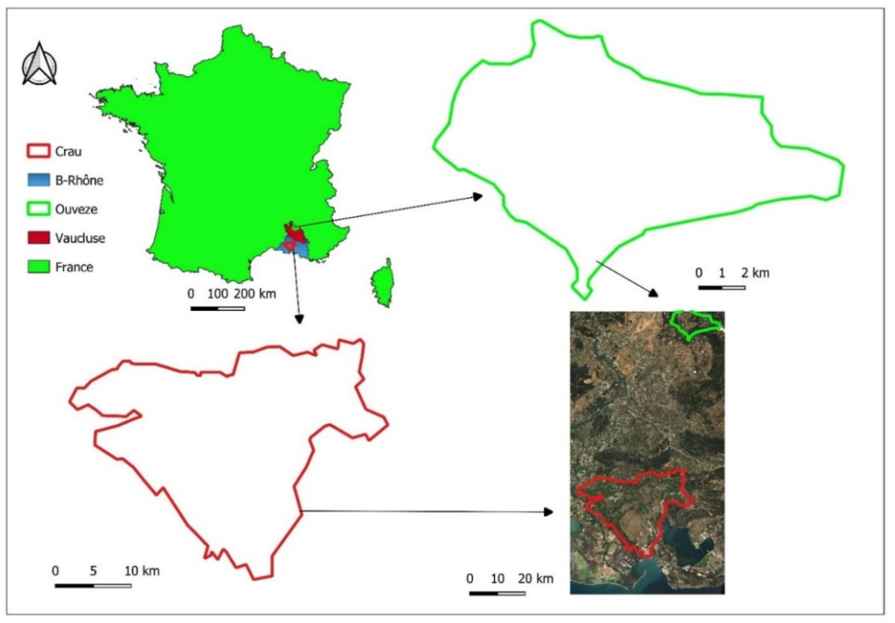
Figure 1.
Map of France depicting the two selected study sites (Ouveze-Ventoux and Crau).
Figure 1.
Map of France depicting the two selected study sites (Ouveze-Ventoux and Crau).
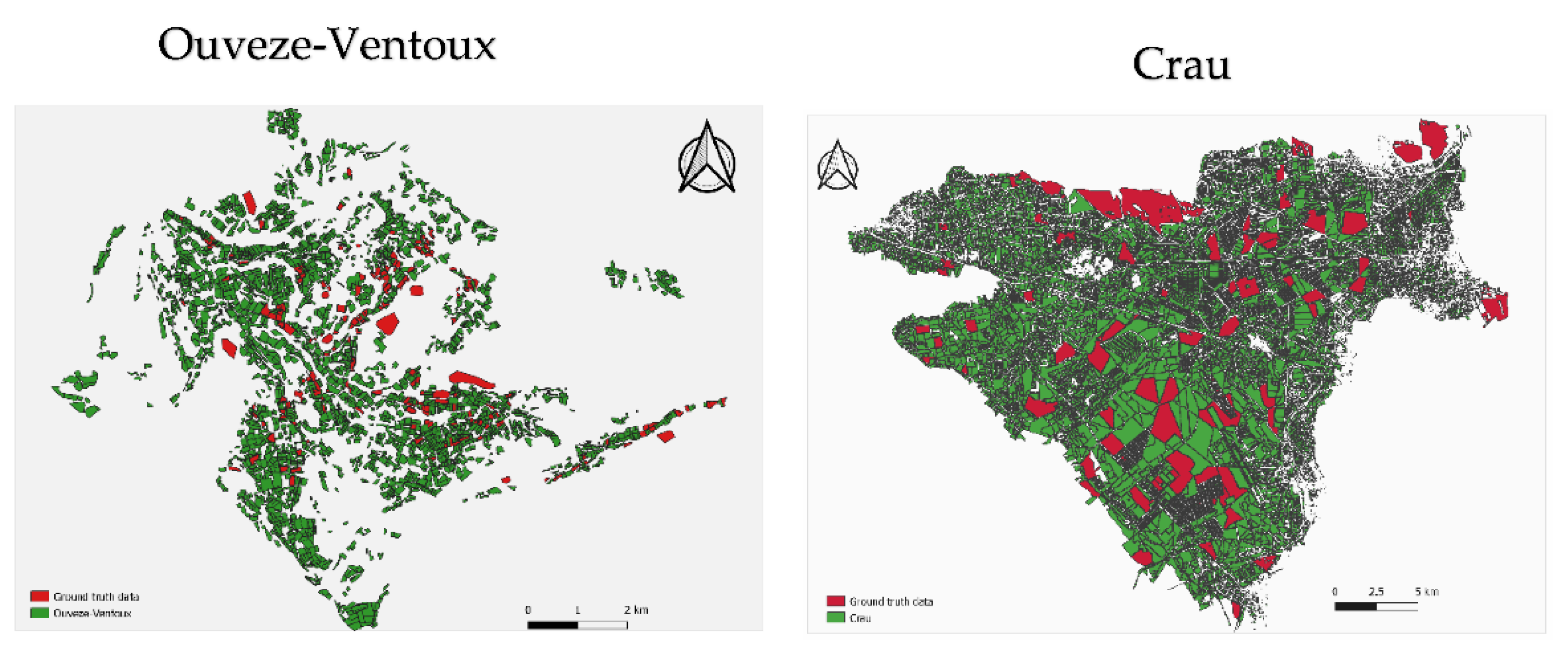
Figure 2.
Map of the two study areas displaying locations of the selected ground truth plot.
Figure 2.
Map of the two study areas displaying locations of the selected ground truth plot.
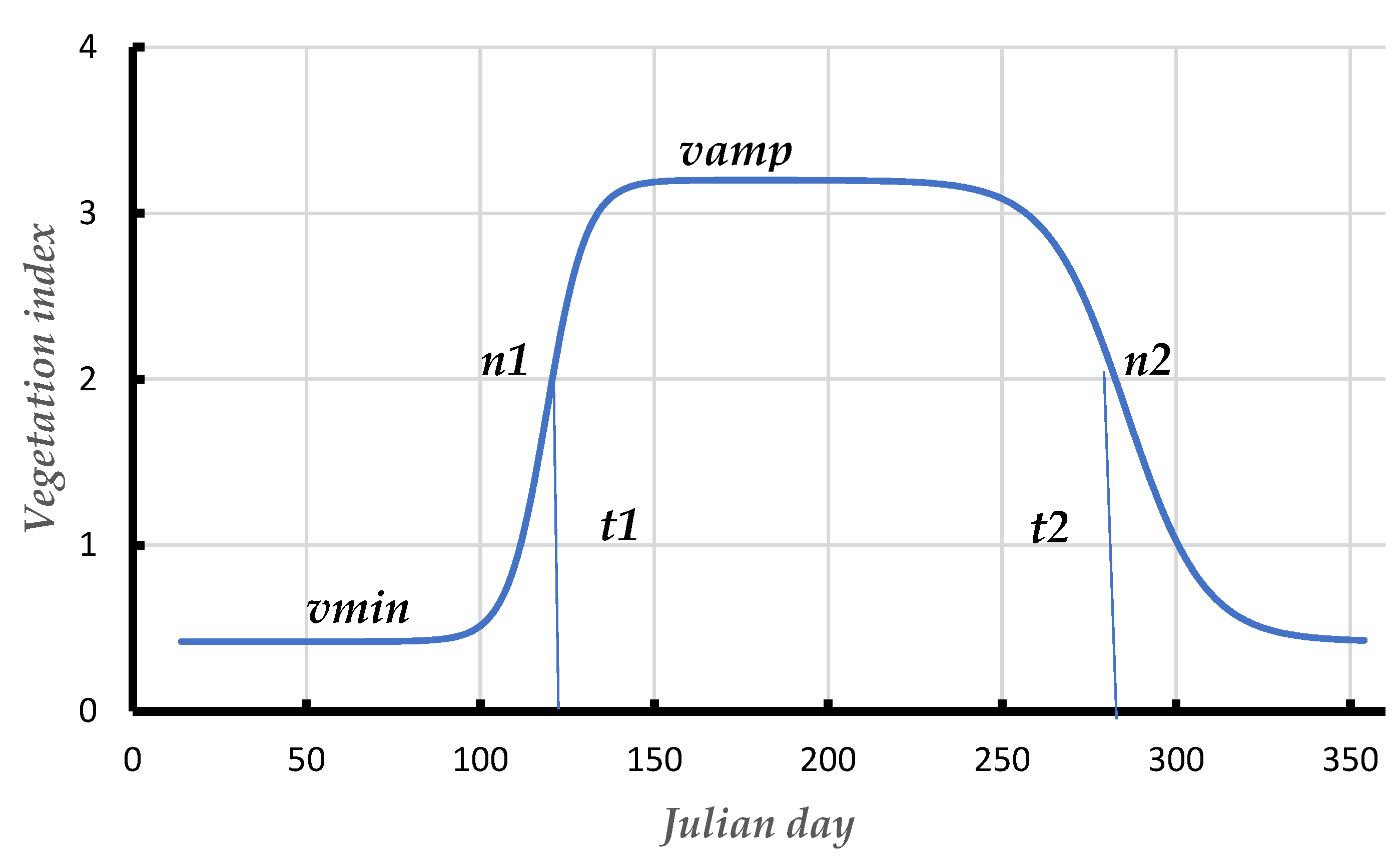
Figure 3.
Double logistic fitting showing SOS and EOS.
Figure 3.
Double logistic fitting showing SOS and EOS.
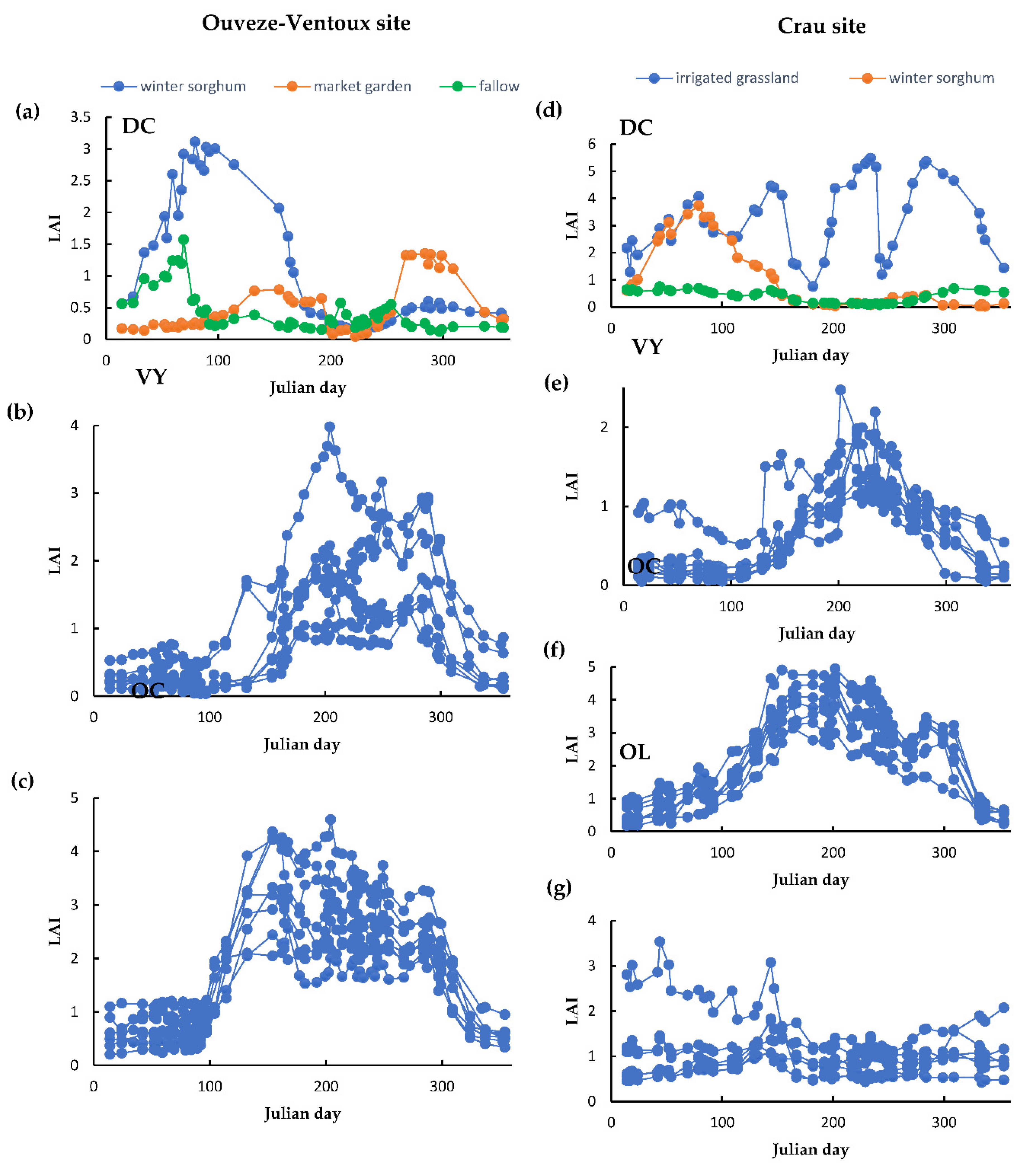
Figure 4.
Temporal profile of DC (a), VY (b), OC (c) s (c) in Ouveze-Ventoux and temporal profile of DC (d), VY (e), OC (f) and OL (g) in Crau site.
Figure 4.
Temporal profile of DC (a), VY (b), OC (c) s (c) in Ouveze-Ventoux and temporal profile of DC (d), VY (e), OC (f) and OL (g) in Crau site.
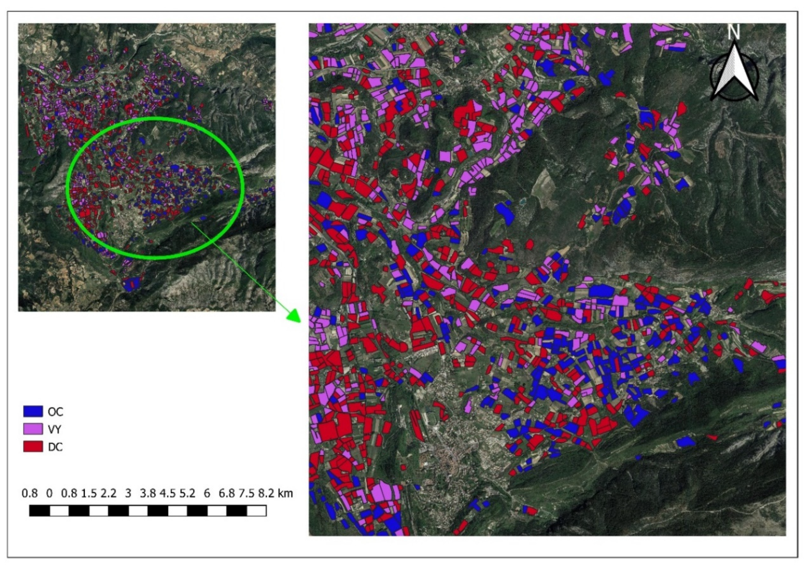
Figure 6.
Spatial distribution of OC, VY, and DC classes in the Ouveze-Ventoux site for the year 2021.
Figure 6.
Spatial distribution of OC, VY, and DC classes in the Ouveze-Ventoux site for the year 2021.
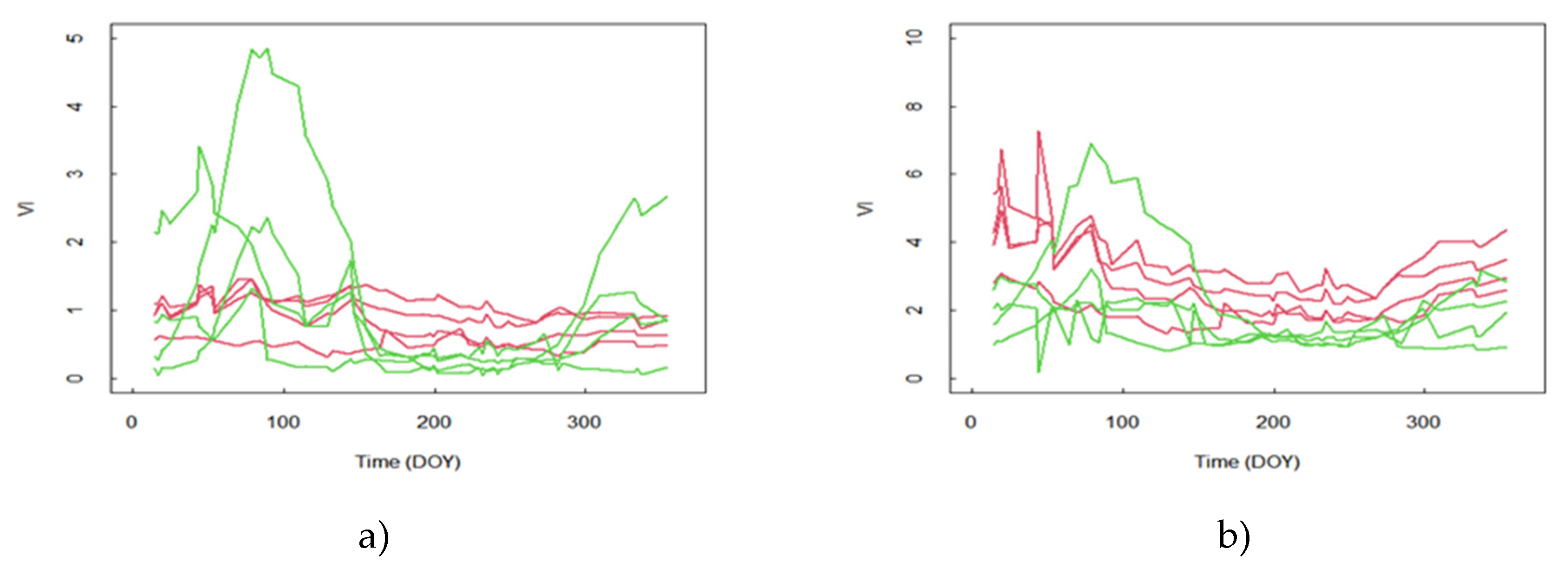
Figure 7.
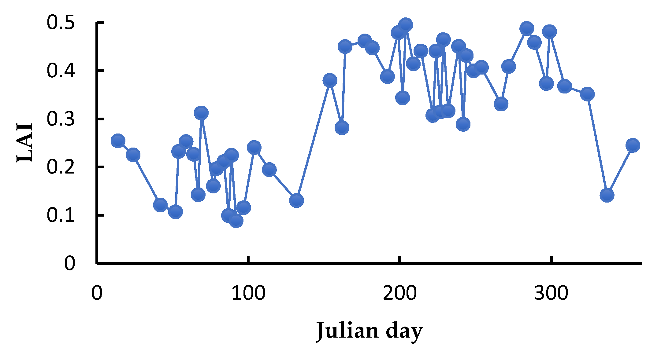
Vegetation Indice time series observed on OL plots (red) and DC (green). In a) the vegetation indices is the LAI, in b) the vegetation indices are GCVI.
Figure 7.
Vegetation Indice time series observed on OL plots (red) and DC (green). In a) the vegetation indices is the LAI, in b) the vegetation indices are GCVI.
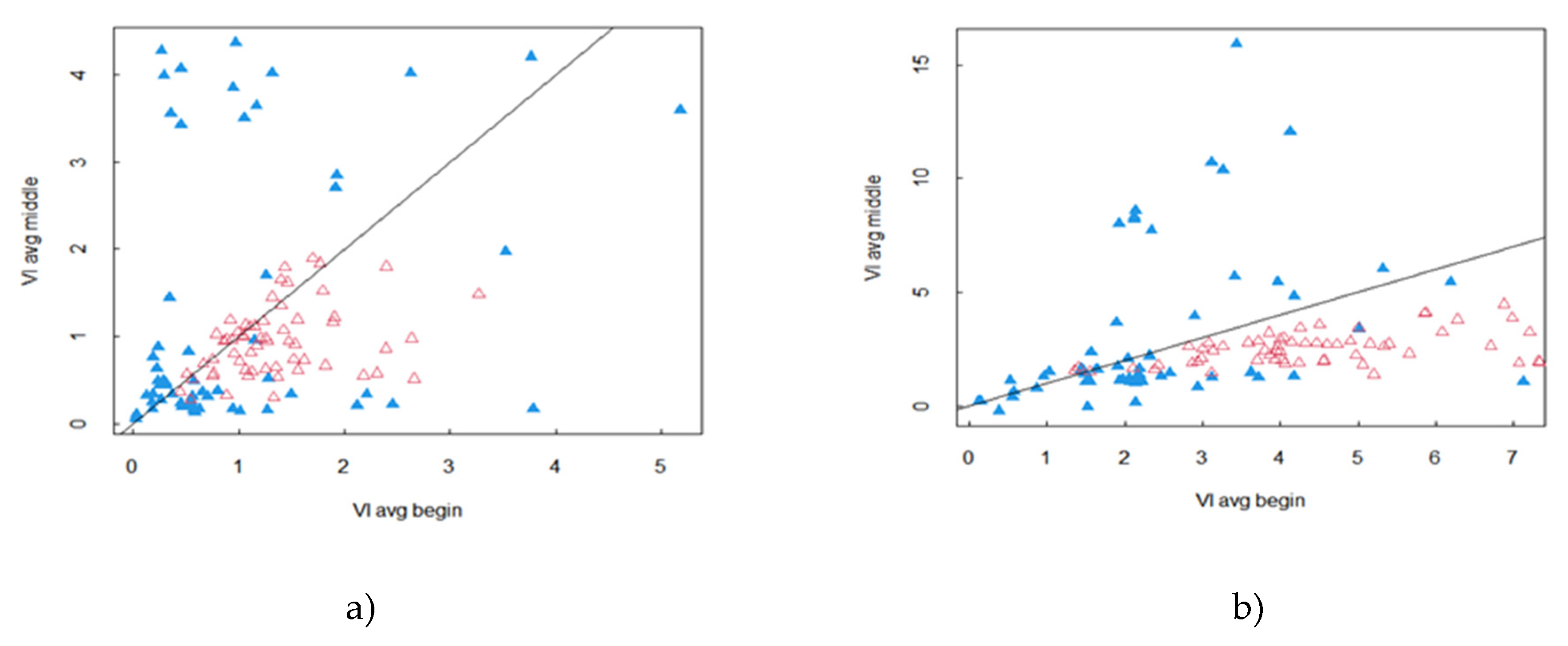
Figure 8.
Average Vegetation indices during the summer period (DOY 150-250) as a function of the average vegetation indices at the beginning of the year (DOY 1-100) for olive plots (red triangle) and end DC plots (blue triangle). In a) the vegetation indices are the LAI and in b) the vegetation indices are GCVI.
Figure 9.
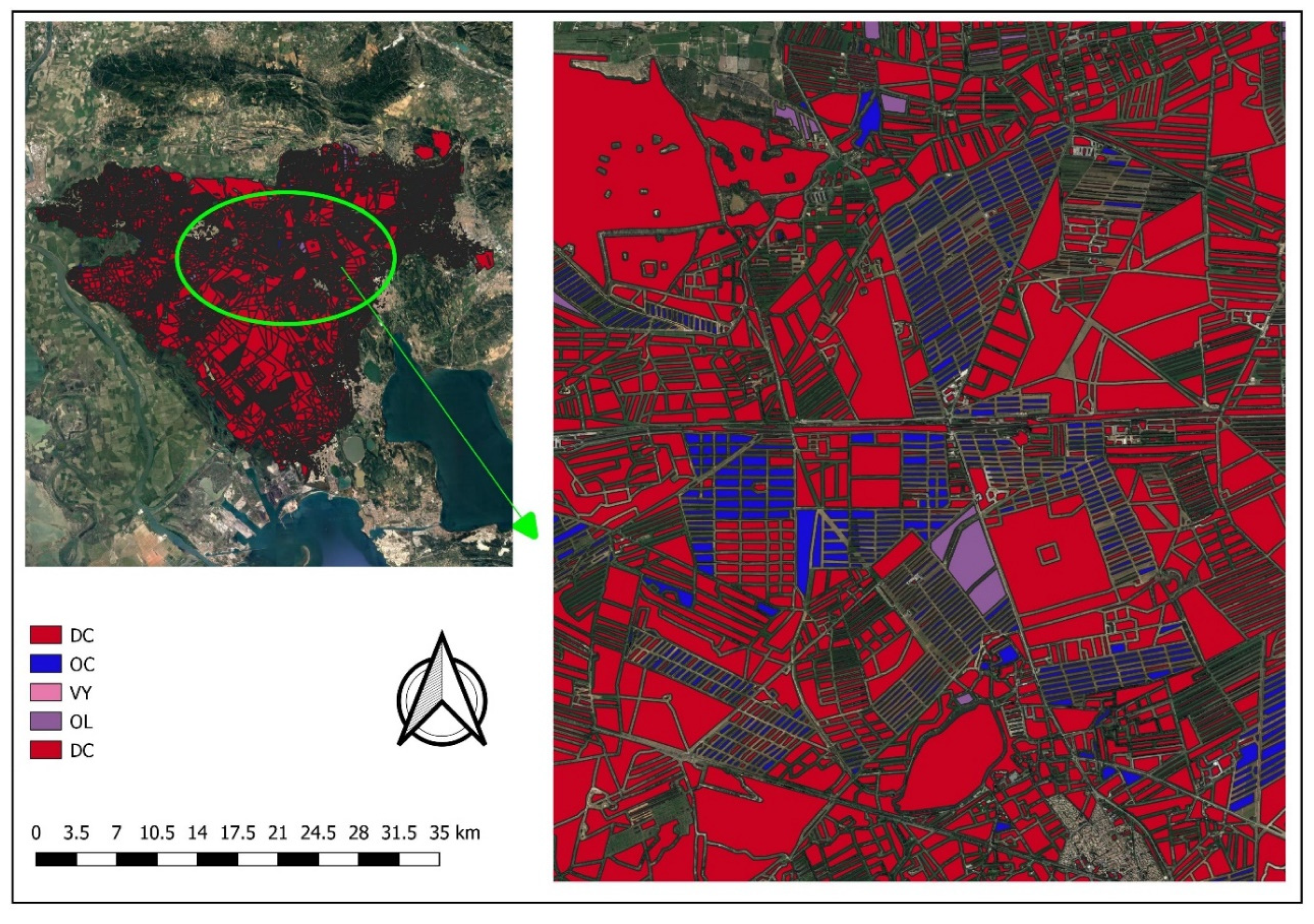
Spatial distribution of OC, VY, OL, and DC classes in Crau.
Figure 9.
Spatial distribution of OC, VY, OL, and DC classes in Crau.
Figure 10.
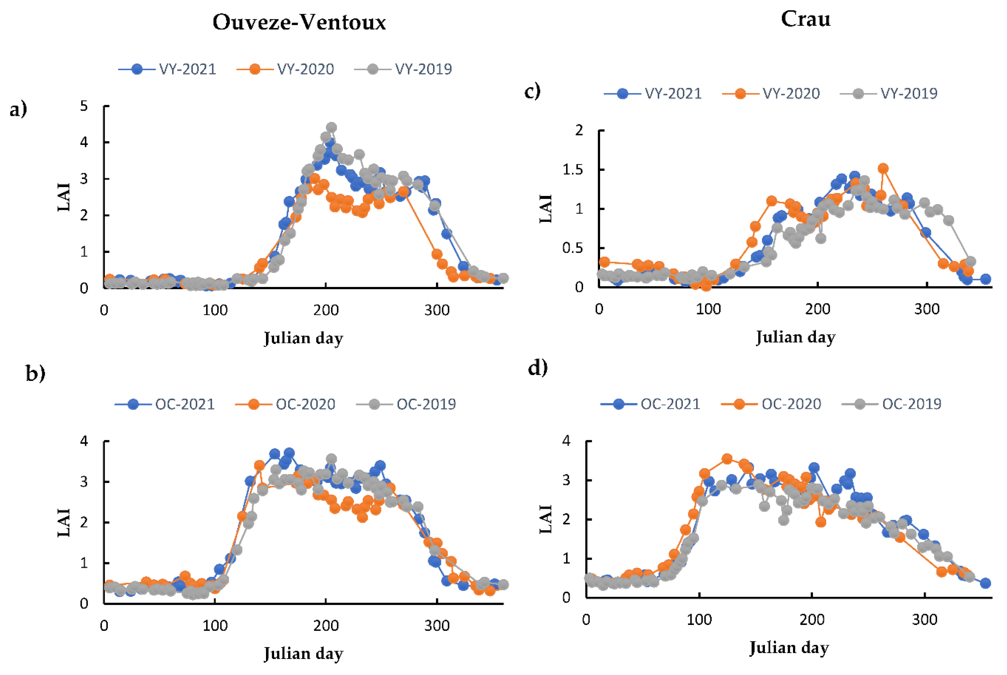
Temporal profile of OC and VY in Ouveze-Ventoux (a and b) and Crau (c and d) study areas from 2019 to 2021.
Figure 10.
Temporal profile of OC and VY in Ouveze-Ventoux (a and b) and Crau (c and d) study areas from 2019 to 2021.
Figure 11.
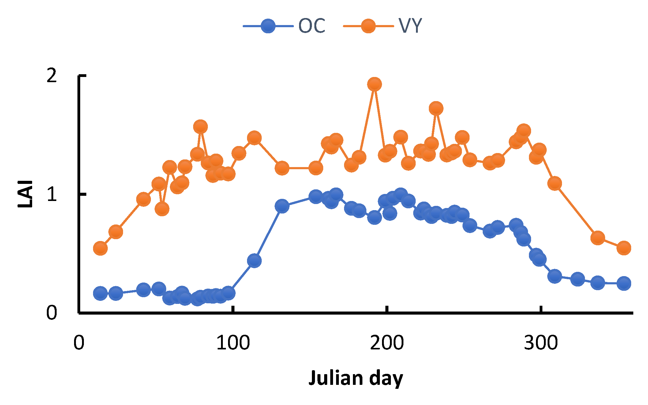
Temporal pattern of a young OC field and a temporal pattern of a young VY.
Figure 11.
Temporal pattern of a young OC field and a temporal pattern of a young VY.
Table 1.
Ground truth information of the two study sites used for model calibration and validation during 2016-2021.
Table 1.
Ground truth information of the two study sites used for model calibration and validation during 2016-2021.
| Ouveze Ventoux site |
Crau site |
| Land use |
Ground data |
Land use |
Ground data |
| |
(number of plots) |
(number of plots) |
| OC |
60 |
OC 88 |
| VY |
100 |
VY 35 |
| OL |
- |
OL 60 |
| DC |
74 |
DC 60 |
Table 2.
Number of cloud-free available images across the two study sites used for the classification.
Table 2.
Number of cloud-free available images across the two study sites used for the classification.
| S/N |
Year |
Ouveze-Ventoux |
Crau |
| 1 |
2016 |
39 |
43 |
| 2 |
2017 |
45 |
49 |
| 3 |
2018 |
52 |
55 |
| 4 |
2019 |
51 |
56 |
| 5 |
2020 |
49 |
52 |
| 6 |
2021 |
50 |
51 |
Table 4.
Classification performance of different vegetation indices and biophysical variables in Ouveze-Ventoux for 2021.
Table 4.
Classification performance of different vegetation indices and biophysical variables in Ouveze-Ventoux for 2021.
| Vegetation Indices |
OA (%) |
K |
| NDVI |
82 |
0.71 |
| GNDVI |
80 |
0.70 |
| EVI |
82 |
0.75 |
| TSAVI |
87 |
0.85 |
| ARVI |
81 |
0.77 |
| GCVI |
73 |
0.70 |
| NDMI |
82 |
0.71 |
| LSWI |
80 |
0.77 |
| |
|
|
| Biophysical variables |
OA (%) |
K |
| LAI |
92 |
0.89 |
| FAPAR |
90 |
0.88 |
| FCOVER |
87 |
0.85 |
Table 5.
Confusion matrix for OC and VY classification using PM of LAI in 2021 (subscript a and p correspond to actual and predicted class, respectively).
Table 5.
Confusion matrix for OC and VY classification using PM of LAI in 2021 (subscript a and p correspond to actual and predicted class, respectively).
| |
DCp
|
OCp
|
VYp
|
Total |
User’s accuracy |
| DCa |
35 |
0 |
2 |
37 |
0.94 |
| OCa |
1 |
29 |
0 |
30 |
0.96 |
| VYa |
5 |
1 |
44 |
50 |
0.88 |
| Total |
41 |
30 |
46 |
117 |
|
| Producers’s accuracy |
0.86 |
0.96 |
0.96 |
|
|
| OA = 0.92 ; K = 0.89 |
Table 6.
Confusion matrix for OC and VY classification using PM from LAI 2021 time series and applying a LAI= 0.5 for OC and VY classes (subscript a and p corresponds to actual and predicted class, respectively).
Table 6.
Confusion matrix for OC and VY classification using PM from LAI 2021 time series and applying a LAI= 0.5 for OC and VY classes (subscript a and p corresponds to actual and predicted class, respectively).
| |
DCp
|
OCp
|
VYp
|
Total |
User’s accuracy |
| DCa |
37 |
0 |
2 |
39 |
0.95 |
| OCa |
0 |
30 |
0 |
30 |
1.00 |
| VYa |
1 |
1 |
46 |
48 |
0.97 |
| Total |
38 |
31 |
48 |
117 |
|
| Producers’s accuracy |
0.95 |
0.96 |
0.95 |
|
|
| OA = 0.96 ; K = 0.91 |
Table 7.
Results of OC and VY classification in Ouveze-Ventoux from 2016-201 based on PM derived from LAI time series and applying LAI = 0.5 thresholds for OC and VY classes.
Table 7.
Results of OC and VY classification in Ouveze-Ventoux from 2016-201 based on PM derived from LAI time series and applying LAI = 0.5 thresholds for OC and VY classes.
| Year |
Site |
Accuracy assessments |
|
| |
|
OA (%) |
Kappa |
| 2016 |
Ouveze-Ventoux |
89 |
0.86 |
| 2017 |
|
90 |
0.89 |
| 2018 |
|
91 |
0.90 |
| 2019 |
|
94 |
0.92 |
| 2020 |
|
95 |
0.93 |
| 2021 |
|
96 |
0.91 |
Table 8.
Confusion matrix for OC, VY, OL, and DC classification based on PM from 2021 time series (subscript a and p correspond to actual and predicted class, respectively).
Table 8.
Confusion matrix for OC, VY, OL, and DC classification based on PM from 2021 time series (subscript a and p correspond to actual and predicted class, respectively).
| |
DCp
|
OCp
|
OLp
|
VYp
|
Total |
User’s accuracy |
| DCa |
19 |
0 |
11 |
0 |
30 |
0.63 |
| OCa |
0 |
42 |
0 |
2 |
44 |
0.95 |
| OLa |
10 |
0 |
20 |
0 |
30 |
0.67 |
| VYa |
11 |
2 |
0 |
5 |
18 |
0.28 |
| Total |
40 |
44 |
31 |
7 |
122 |
|
| Producers’s accuracy |
0.50 |
0.95 |
0.65 |
0.71 |
|
|
| |
OA = 0.70 ; K = 0.69 |
Table 9.
Confusion matrix for OC and VY classification based on PM from 2021 LAI time series and after gathering OC and DC in common DC class (subscript a and p correspond to actual and predicted class, respectively).
Table 9.
Confusion matrix for OC and VY classification based on PM from 2021 LAI time series and after gathering OC and DC in common DC class (subscript a and p correspond to actual and predicted class, respectively).
| |
DCp
|
OCp
|
VYp
|
Total |
User’s accuracy |
| DCa |
60 |
0 |
0 |
60 |
1.00 |
| OCa |
0 |
44 |
0 |
44 |
1.00 |
| VYa |
6 |
1 |
11 |
18 |
0.61 |
| Total |
66 |
45 |
11 |
122 |
|
| Producers’s accuracy |
0.91 |
0.98 |
1.00 |
|
|
| OA = 0.94 ; K = 0.91 |
Table 10.
Same as
Table 9 with an additional threshold of LAI=1 for OC and VY classes of LAI in 2021 (subscript a and p correspond to actual and predicted class, respectively).
Table 10.
Same as
Table 9 with an additional threshold of LAI=1 for OC and VY classes of LAI in 2021 (subscript a and p correspond to actual and predicted class, respectively).
| |
DCp
|
OCp
|
VYp
|
Total |
User’s accuracy |
| DCa |
62 |
0 |
0 |
62 |
1.00 |
| OCa |
0 |
44 |
0 |
44 |
1.00 |
| VYa |
3 |
1 |
12 |
16 |
0.75 |
| Total |
65 |
45 |
12 |
122 |
|
| Producers’s accuracy |
0.95 |
0.98 |
1.00 |
|
|
| OA = 0.97 ; K = 0.95 |
Table 11.
Confusion matrix for DC and OL classification based on a temporal feature from 2021 GCVI time series (subscript a and p correspond to actual and predicted class, respectively).
Table 11.
Confusion matrix for DC and OL classification based on a temporal feature from 2021 GCVI time series (subscript a and p correspond to actual and predicted class, respectively).
| |
DCp
|
OLp
|
Total |
User’s accuracy |
| DCa |
25 |
5 |
30 |
0.87 |
| OLa |
1 |
29 |
30 |
0.97 |
| Total |
26 |
34 |
60 |
|
| Producers’s accuracy |
0.96 |
0.88 |
|
|
| OA = 0.91 ; K = 0.82 |
Table 12.
Results of OL classification in Crau from 2016-201 using GCV.
Table 12.
Results of OL classification in Crau from 2016-201 using GCV.
| Year |
Site |
Accuracy assessments |
|
| |
|
OA (%) |
Kappa |
| 2016 |
Crau |
90 |
0.86 |
| 2017 |
|
90 |
0.88 |
| 2018 |
|
95 |
0.93 |
| 2019 |
|
93 |
0.92 |
| 2020 |
|
94 |
0.91 |
| 2021 |
|
97 |
0.94 |
Table 13.
Confusion matrix of DC, OC, OL and, VY classification in Crau for 2021.
Table 13.
Confusion matrix of DC, OC, OL and, VY classification in Crau for 2021.
| |
DCp
|
OCp
|
OLp
|
VYp
|
Total |
User’s accuracy |
| DCa |
31 |
0 |
1 |
0 |
32 |
0.97 |
| OCa |
0 |
44 |
0 |
0 |
44 |
1.00 |
| OLa |
1 |
0 |
29 |
0 |
30 |
0.97 |
| VYa |
3 |
1 |
0 |
12 |
16 |
0.75 |
| Total |
35 |
45 |
30 |
12 |
122 |
|
| Producers’s accuracy |
0.89 |
0.98 |
0.97 |
1.00 |
|
|
| |
OA = 0.96 ; K = 0.95 |
Table 14.
Results of OC, VY, OL global classification accuracy in Crau from 2016-201.
Table 14.
Results of OC, VY, OL global classification accuracy in Crau from 2016-201.
| Year |
Site |
Accuracy assessments |
|
| |
|
OA (%) |
Kappa |
| 2016 |
Crau |
89 |
0.87 |
| 2017 |
|
90 |
0.87 |
| 2018 |
|
92 |
0.90 |
| 2019 |
|
94 |
0.91 |
| 2020 |
|
93 |
0.91 |
| 2021 |
|
96 |
0.95 |
Table 15.
Classification performance of the raw spectral satellite images (LAI) across the two study sites for OC and VY using RF classifier.
Table 15.
Classification performance of the raw spectral satellite images (LAI) across the two study sites for OC and VY using RF classifier.
| Year |
Site |
OA (%) |
K |
| 2016 |
Ouveze-Ventoux |
43 |
0.30 |
| 2017 |
|
47 |
0.32 |
| 2018 |
|
55 |
0.41 |
| 2019 |
|
51 |
0.49 |
| 2020 |
|
55 |
0.51 |
| 2021 |
|
52 |
0.50 |
| |
|
|
|
| 2016 |
Crau |
41 |
0.32 |
| 2017 |
|
45 |
0.31 |
| 2018 |
|
49 |
0.41 |
| 2019 |
|
55 |
0.52 |
| 2020 |
|
60 |
0.51 |
| 2021 |
|
58 |
0.49 |
Table 16.
THEIA classification performance across the two study sites for OC and VY using RF classifier and other supplementary data.
Table 16.
THEIA classification performance across the two study sites for OC and VY using RF classifier and other supplementary data.
| Year |
Site |
OA (%) |
Kappa |
| 2016 |
Ouveze-Ventoux |
73 |
0.70 |
| 2017 |
|
77 |
0.72 |
| 2018 |
|
75 |
0.71 |
| 2019 |
|
78 |
0.75 |
| 2020 |
|
75 |
0.71 |
| 2021 |
|
72 |
0.69 |
| |
|
|
|
| 2016 |
Crau |
76 |
0.73 |
| 2017 |
|
75 |
0.69 |
| 2018 |
|
79 |
0.75 |
| 2019 |
|
75 |
0.72 |
| 2020 |
|
73 |
0.68 |
| 2021 |
|
78 |
0.75 |
Table 17.
Classification performance using PM for classifying orchards and vineyards applying the predicted model of 2021 across years and sites.
Table 17.
Classification performance using PM for classifying orchards and vineyards applying the predicted model of 2021 across years and sites.
| Accuracy Assessment |
|---|
| |
Calibrated RF model |
2021 model across years |
| Year |
Site |
OA |
Kappa |
OA |
Kappa |
| 2016 |
Ouveze-Ventoux |
0.89 |
0.86 |
81 |
0.72 |
| 2017 |
|
0.90 |
0.89 |
83 |
0.76 |
| 2018 |
|
0.91 |
0.90 |
82 |
0.79 |
| 2019 |
|
0.94 |
0.92 |
83 |
0.81 |
| 2020 |
|
0.95 |
0.93 |
86 |
0.85 |
| 2016 |
Crau |
89 |
0.87 |
83 |
0.79 |
| 2017 |
|
90 |
0.87 |
82 |
0.78 |
| 2018 |
|
92 |
0.90 |
85 |
0.80 |
| 2019 |
|
94 |
0.91 |
87 |
0.83 |
| 2020 |
|
93 |
0.91 |
86 |
0.80 |
| |
Calibrated RF model |
2021 model across sites |
| 2021 |
Ouveze Ventoux |
96 |
0.91 |
71 |
0.65 |
| 2021 |
Crau |
89 |
0.87 |
60 |
0.51 |
