
You are currently viewing a beta version of our website. If you spot anything unusual, kindly let us know.
Preprint
Article
Mapping Malaria Vectors in West Africa: Drone Imagery and Deep-Learning Analysis for Targeted Vector Surveillance
Altmetrics
Downloads
169
Views
137
Comments
0
A peer-reviewed article of this preprint also exists.


This version is not peer-reviewed
Abstract
Disease control programs need to identify breeding sites of mosquitoes which transmit malaria and other diseases to target interventions and identify environmental risk factors. Increasing availability of very high resolution drone data provides new opportunities to find and characterize these vector breeding sites. Within this study, we identified land cover types associated with malaria vector breeding sites in West Africa. Drone images from two malaria endemic regions in Burkina Faso and Côte d’Ivoire were assembled and labeled using open-source tools. We developed and applied a workflow using region of interest-based and deep learning methods to classify these habitat types from very high resolution natural color imagery. Analysis methods achieved a dice coefficient ranging between 0.68 and 0.88 for different vector habitat types; however, this classifier consistently identified the presence of specific habitat types of interest. This establishes a framework for developing deep learning approaches to identify vector breeding sites and highlights the need to evaluate how results will be used by control programs.
Keywords:
Subject: Computer Science and Mathematics - Artificial Intelligence and Machine Learning
1. Introduction
Land-use changes, such as agricultural expansion, can create new aquatic habitats suitable for breeding sites for mosquito vectors that transmit malaria and other diseases [1]. When aquatic mosquito habitats can be identified, disease control programs can implement targeted interventions such as larval source management, reducing mosquito densities through chemical, biological, or environmental means [2]. While traditional approaches relied on ground-based surveys, Earth Observation (EO) data, such as drone and satellite data, is increasingly utilized to identify potential breeding sites rapidly and target control measures [3,4,5,6,7]. EO data additionally provides new opportunities to characterize mosquito habitats and monitor changes in these habitats in response to environmental change [8].
Obtaining actionable information from EO data requires classifying imagery into relevant habitat types. The specific classes of interest are highly dependent on local vector ecology; for example, Anopheles funestus, the second most important malaria vector in Africa, commonly breeds in large, vegetated water bodies [9,10,11,12]. In contrast, An. gambiae breed in small or temporary, often man-made water bodies across a wide range of habitat types, including roads, agricultural irrigation such as rice paddies, sunlit rivers and streams, and quarries or construction sites [2,13,14]. Additionally, the type of information required when classifying EO data depends on the end-use. While a vector control program may benefit from knowing the probability of a large area containing habitat types, ecological and epidemiological studies may require more detailed segmentation approaches to characterize the shape and configuration of different habitat types [15,16,17,18,19,20,21].
For these applications, it is critical that EO data is collected simultaneously as ground-based vector surveys or is recent enough to provide actionable information for control programs. This has led to increased use of EO data with high spatial and temporal resolutions, such as user-defined imagery collected by drone (unmanned aerial vehicles or UAVs) or daily commercial satellite data (e.g., Planet). These data typically have a low spectral resolution, limiting the utility of traditional pixel-based approaches requiring data measured outside the visible spectrum [22,23]. Alternatively, deep learning approaches, such as convolutional neural networks (CNNs), have revolutionized image analysis by efficiently analyzing image textures, patterns, and spectral characteristics using self-learning artificial intelligence approaches to identify features in complex environments [20,24,25,26].
Multiple approaches have been applied for identifying habitats and their characteristics from EO imagery for operational use by vector-borne disease control programs. In Malawi, Stanton et al. [7] assessed approaches for identifying the aquatic habitats of larval-stage malaria mosquitoes. They assessed geographical object-based image analysis (GeoOBIA), a method that groups contiguous pixels into objects based on prespecified pixel characteristics. The objects were classified by a random forest supervised classification and demonstrated strong agreement with test samples, successfully identifying larval habitat characteristics with a median accuracy of 98%. Liu et al. [27] developed a framework for mapping the spatial distribution of suitable aquatic habitats for the snail hosts of the debilitating parasitic disease Schistosomiasis along the Senegalese River Basin. A deep learning U-Net model was built to analyze high-resolution satellite imagery and to produce segmentation maps of aquatic vegetation. The model produced predictions of snail habitats with higher accuracy than commonly used pixel-based classification methods such as random forest. Hardy et al. [28] developed a novel approach to classify and extract malaria vector larval habitats from drone imagery in Zanzibar, Tanzania. This used computer vision to assist manual digitization. This approach was found to significantly outperform supervised classification approaches, which were unsuitable for mapping potential vector larval habitats in the study region based on accuracy scores.
For other applications, a range of analysis approaches has been developed to identify features from drone imagery [29]. For example, gray-level co-occurrence matrix (GLCM) techniques for vegetation structure modeling have been applied to reduce noise and improve the classification of UAV images by using textural information [29]. Similarly, Hu et al. [30] proposed a two-step approach coupling classification and regression trees to estimate the ground coverage of wheat crops from UAV imagery with coarse spatial resolutions. First, a classification tree-based per-pixel segmentation was applied to segment fine-resolution reference images into binary reference images of vegetated and non-vegetated areas. Next, a regression-tree-based model was used to develop sub-pixel classification methods. This two-step approach increased classification accuracy on both real and synthetic image datasets. Other studies have explored the utility of using spectral data to monitor land cover changes using very high-resolution imagery. For example, Komarkova et al. [31] calculated eight vegetation indices calculated from red, green, and blue (RGB) UAV imagery with a 1.7 cm per pixel resolution; indices were identified, which allowed the identification of vegetated and clear water surfaces. This high-resolution RGB data can also be integrated with satellite imagery with higher spectral resolution and lower spatial resolution. For example, Cao et al. [32] applied a multiple criteria spectral mixture analysis (MCSMA) to map fractional urban land covers (vegetation, impervious surface, and soil) on Landsat-8 surface reflectance imagery (30 m/pixel, seven optical bands) with high-resolution RGB data from Google Earth using a multistep process. First, the authors obtain spectrally pure patches through minimum distance, maximum likelihood, and support vector machine classifiers. Mixed pixels at boundary regions of the patches were removed by applying the morphological erosion operation, and the centroid of each patch was computed to form end member candidates. Then, the MCSMA constructs all possible end member models using a spatially adaptive strategy. All possible end member models were finally tested for the target pixel using a constrained linear spectral unmixing method to improve classification accuracy. Rustowicz et al. [33] compare the performance between a 3D U-Net with a 3x3 kernel followed by batch norm and a leaky Rectified Linear Unit (ReLU) activation and well-known models incorporating both CNNs and recurrent neural networks (RNN) for semantic segmentation of multi-temporal, multi-spatial satellite images. Sentinel 1, Sentinel 2, and Planet satellite imagery of sparse ground truth labels of crop fields in South Sudan and northern Ghana were used in this contribution. In addition, a German dataset was used in the comparison. Ground truth labels consist of geo-referenced polygons, where each polygon represents an agricultural field boundary with a crop type label, including maize, groundnut, rice, and soya bean. As a part of the experimental process, the authors performed a hyperparameter search across optimization methods through Adam and SGD techniques. The authors find that models trained on the German dataset outperformed models tested on South Sudan and Ghana datasets. Smaller training sets, high cloud cover, and complex landscapes in the smallholder setting affected the results obtained.
Building on these methods, we aimed to develop and validate deep learning approaches to identify land classes associated with the breeding sites of malaria mosquito vectors in West Africa. Data were assembled from multiple sites in Burkina Faso and Côte d’Ivoire to develop an approach able to generalize to different malaria-endemic landscapes. We used RGB drone images from the study sites to build a training dataset and to implement two CNN-based frameworks using the U-Net and attention U-Net architectures to identify features of interest for Anopheles breeding ecology. The specific objectives of this study were to (i) collect and assemble a dataset of drone images in malaria-endemic areas in Côte d’Ivoire and Burkina Faso; (ii) develop the protocol to label land classes of interest in drone imagery; (iii) assemble a labeled dataset for each class and (iv) train, validate and test U-net and attention U-net deep learning architectures. Final algorithms were assessed based on the performance of predicting the presence of the classes of interest in test images using the best model after cross validation.
2. Materials and Methods
2.1. Drone mapping
Drone surveys were conducted in two malaria endemic sites in West Africa: Saponé, Burkina Faso and Bouaké, Côte d’Ivoire where the incidence of malaria (per 1000 population at risk) are 389.9 and 2871, respectively. Both sites are rural with extensive small-scale agriculture and highly seasonal rainfall and malaria transmission patterns. Saponé is located 45 km south-west of Ouagadougou, Burkina Faso and has reported extremely high malaria prevalence of predominantly Plasmodium falciparum [34]. The main malaria in this site is An. gambiae s.l., with low densities of other species also reported. Between November 2018 - November 2019, fixed wing (Sensefly eBee) and quadcopter (DJI Phantom 4 Pro) drones were used to collect RGB data at 2-10cm per pixel resolution. Similarly, in Bouaké, we conducted targeted drone surveys from June - August 2021 using a DJI Phantom 4 Pro drone to collect RGB data at a 2cm per pixel resolution as described by [6]. This area was also rural and dominated by small scale agriculture; however, this site had different vector compositions, including high densities of An. funestus. For both sites, drone images were processed using Agisoft Metashape Professional2 to generate orthomosaics. The drone images cover 11.52 km2 and 30.42 km2 area for Burkina Faso and Côte d’Ivoire, as illustrated in Figure 1. Both sites were dominated by agriculture, mainly yams, cassava, cashew, peanuts, and maize.
2.2. Image Labeling and Development of Labeled Dataset
We identified specific land cover classes of interest associated with Anopheles breeding sites, including water bodies and irrigated agricultural land types [6]. We differentiated between vegetated and non-vegetated water bodies as An. funestus is most commonly identified only in vegetated water bodies. We additionally identified habitat types not associated with Anopheles breeding sites but with human activities, including roads and buildings. The final land cover classes of interest for this analysis included vegetated and non-vegetated water bodies, irrigated crops (planted vegetation with no tree cover), tillage (land cleared for planting crops), buildings and roads. While this classification cannot specifically identify whether or not an area is an Anopheles breeding site, this provides the basis for targeting future entomological surveys and wider epidemiological studies on how landscape impacts malaria transmission.
To identify these classes using a supervised deep learning approach, we first needed to assemble a dataset of harmonised labelled images. We manually labelled all drone acquisitions to generate gold standard (i.e., labeled images) masks for each of the specific land classes. Trained personnel familiar with the study area validated the labels. This process was performed using two different tools: QGIS3 and GroundWork4. The former is a Geographic Information System (GIS) open-source desktop application that allows inputting geo-referenced images and annotating manually using polygons (Figure 2). Groundwork, on the other hand, is a cloud-based licensed tool where the images are uploaded for labelling. In this cloud-based interface, a grid is overlaid in the image as illustrated in Figure 3A. The user is then able to select one of the predefined classes to assign the corresponding class over the images as shown in Figure 3B. While this tool has a streamlined workflow to facilitate labelling, this required internet access, had a limited data allowance and was not suitable in all contexts. The obtained polygons from both tools were checked to detect invalid polygons and were corrected manually.
Once all the images were labeled, ground-truth masks were created for the supervised image classification. As shown in Figure 4, first, we create a subset of vector layers, one for each class. Then, we rasterized the vector layers to create a separate raster image for each class. The land class presence depended on the acquisition site’s characteristics. For example, Figure 5 shows a labeled region from Burkina Faso where all the land classes are present; however, this is not the case for all the images. Images that did not contain labeled polygons were not considered in this study.
We built six land class datasets: crops, tillage, roads, buildings, vegetated water bodies and non-vegetated water bodies (defined at the beginning of this section). For each dataset, we selected only the drone images that contained labels of the corresponding land class. From each dataset we randomly selected images for training, validation and test. To avoid bias related to the training data, we considered using a 3-fold cross-validation scheme.
Due to GPU memory constrains, the entire drone image and its corresponding labels were split into several patches, which were used to train, validate and test the deep learning models. In addition, because of the variable extension of each labeled polygon, splitting the image in a grid pattern resulted in a highly unbalanced dataset where the background predominated over the class of interest. Instead, we used a new approach for data patching and augmentation based on ROI-shifting, described in [35], to avoid this imbalance. This method also prevented potential bias caused by the network focusing on the background instead of the class of each patch. The augmentation aimed to train the models robustly in the presence of variable neighborhood context information. Thus, we identified the ROIs and frame them in rectangles, which could contain one or more polygons as illustrated in Figure 6. Patches of sizes 256×256 and 512×512 pixels were extracted from those rectangles and assigned to each training, validating and testing datasets. A summary of the number of images and patches in each dataset is reported in Table 1. For each patch size, we report in Table 2 the average percentage of the class present in the dataset. This is computed, per patch, as the ratio of the pixels belonging to each class and the background pixels. Patches with classes representing less than 10% (256×256) or 20% (512×512) of the patch size were eliminated from the datasets. The total number of patches obtained for each class differs by study site; while Burkina Faso contained more tillage areas, Côte d’Ivoire had more irrigated crops. Considering both sites, water body datasets contained the least number of patches. On average, non-vegetated water bodies, tillage, and crops covered greater percentages of patches as these classes were more likely to be larger.
2.3. Algorithm Development
We developed a multi-step approach to classifying multiple land classes from patches, as shown in Figure 6. Following the dataset preparation, two deep learning segmentation models were selected: U-net and attention U-Net. The U-Net is a widely used architecture for semantic segmentation tasks. This method relies on the upsampling technique, which increases an image’s dimension (i.e., the number of rows and/or columns). Thus, the present method builds on a conventional network with successive layers by using upsampling operators to replace pooling operations, which implies using contraction and expansion paths (i.e., encoder and decoder respectively). The contraction part reduces the spatial dimensions in every layer and increases the channels. Meanwhile, the expansive part increases the spatial dimensions while reducing the channels. Finally, using also skip connections between the encoder and decoder, the spatial dimensions are restored to predict each pixel in the input image. An important modification in the U-Net is that many feature bands are in the upper sampling part, allowing the network to propagate context information to higher-resolution layers. Consequently, the expanding trajectory is more or less symmetric to the contracted part and produces a U-shaped architecture [36]. Attention U-Net adds a self-attention gating module in every skip connection of the U-Net architecture without increasing computation overhead. These modules are incorporated to improve sensitivity, accuracy, and add visual explanability to the network. The improvement is performed by focusing on the features of the regions of interest rather than the background [37,38].
Regarding the computational features used in this study, data preparation and deep learning experiments were executed on an 8-core Intel(R) Xeon E5-2686 @ 2.3 GHz CPU with 60 GiB RAM and one 16 GiB RAM Nvidia Tesla V100 GPU on Amazon Elastic Compute Cloud service (AWS).
2.4. Evaluation metrics
To quantitatively assess the similarities between the predicted and gold standard object areas, we used the dice coefficient. This divides two times the area of overlap by the total number of pixels in both images, as shown in Equation 1.
The dice coefficient takes values from 0 to 1, in which 1 represents a complete match between the ground-truth and the prediction. We additionally calculated the precision and recall metrics which are computed based on true positives (TP), false positives (FP), true negatives (TN), and false negatives (FN) as described in equations 2, and 3 respectively.
Based on the aforementioned elements, we performed different experiments that are described in the following section.
3. Results
As the number of ROIs in every drone image was not the same, the number of patches (generated from the ROIs) in each fold varied from class to class. As a result, we used up to 90% of the CPU RAM capacity in the experiments containing the higher number of patches. This computational load was due to caching the data and annotations in CPU RAM prior to moving the batches to the GPU RAM in the training, validation, and test phases. This approach reduces the number of CPU-GPU data transfers which can intensively impact the training time. The average training and cross-validation time was approximately 12 hours.
The U-Net and attention U-Net architectures were used to classify the different classes organized in sets of patches of 256×256 and 512×512 pixels in size using a 3-fold cross-validation procedure. Table 3 shows the results for the U-Net using patches with a size of 256×256 pixels. For vegetated water bodies, one of our primary classes of interest, the model reached its highest dice score at 0.68 in the first fold and an average of 0.63. Non-vegetated water bodies had a higher dice score of 0.75 and 0.58 on average, showing the worst performance among all the classes. Crops, tillage, and buildings had the best overall performance, above 0.80 in all validation sets, followed by roads that reached 0.71. The same U-Net architecture was also trained with patches of 512x512 pixels in size. For both training approaches, all classes achieved comparable results; however, the model trained with 256x256 pixel size patches outperformed, on average, the 512×512 model in every class. The detailed table showing the performance of the 512×512 pixels size model is in the Supplementary Information.
Similarly to the U-Net experiments, we trained the attention U-Net with patches of 256x256 pixels. The evolution of the training is shown in Figure 7. The areas where the network finds relevant features for segmentation are displayed in red, while the blue areas correspond to less essential regions. The first column shows the original patch, and the following columns are the heatmaps according to an iteration number indicated above; however, they correspond to different epochs. In general, for non-vegetated water body (Figure 7c), roads (Figure 7d), and vegetated water body (Figure 7f) patches, we notice that, as the number of iterations increases, the network focuses more on the areas of interest for learning. Nevertheless, in the case of buildings (Figure 7a), the initial iteration focuses more on the construction than the final one because it corresponds to a different epoch and batch, meaning that iteration 212 corresponds to an early epoch where the network is not fully updated or a batch with different data distribution than the patch analyzed. Another important highlight is that in some iterations, the network concentrates not on the class but in the shadows of the patch, such as in Figure 7d iteration 327 and Figure 7d iteration 3.
The quantitative results to evaluate the performance of the attention U-Net using patches of 256×256 pixels are reported in Table 4. Comparing these results with the ones obtained with the 256×256 U-Net model, we observe that the vegetated and non-vegetated water body classes have improved performance. Despite that, the first fold of the non-vegetated water body class showed a low dice performance (below 5%), meaning the training is unstable across the 3 folds and may impact the inference process due to different data distributions present in the datasets. Therefore, cross-validation provided insights into the robustness and stability of the trained models.
We also trained the attention U-Net using patches of 512×512 pixels. However, we used a subset of patches per class ranging from 5% to 20% to test the model performance on the vegetated and non-vegetated water bodies, crops, and buildings classes. Even though it shows an improvement in the water body classes compared to the 256×256 pixels U-Net model using the best fold as a reference, the standard deviation calculated after the cross-validation is higher, meaning the network is not entirely stable. For instance, in the non-vegetated class, the dice score ranges from 0.1 to 0.91 in the attention U-Net 512×512 pixels model. We reported all results for this last experiment in the Supplementary Information.
We selected the U-Net 256×256 pixels model to evaluate the predicted maks as it was the most stable and robust network. Figure 8 shows the inference results for one sample patch (taken from the test dataset) per class. The first column shows the original test patch. The second column shows the gold standard in white and the background in black, whereas the third column is the network prediction, where each pixel is depicted in white if it belongs to the corresponding class with a probability higher than 0.65. The patch’s dice score is reported above each predicted mask.Figure 8a shows the buildings accurately distinguished over the soil region. In contrast, qualitative results for crop class in Figure 8b show that the network predicts as crops more regions of soil between the leaves rather than the actual crop. This may be explained due to the imprecise annotations (i.e., mask almost covering 100% of the patch area) seen in the gold standard. Figure 8c presents a water body’s segmentation despite the shadows and blurriness of the patch. Figure 8d, a show a road and a vegetated water body, respectively. In both cases, the network outperformed the manual annotation qualitatively. Finally, the tillage model output shown in Figure 8e predicts not only the corresponding class but also areas of soil that were not prepared for cultivation.
4. Discussion
This study highlights the utility of deep learning approaches to identify potential mosquito habitats using high-resolution RGB imagery. We developed a workflow and methodology to assemble and process labeled training data to implement deep learning algorithms to automatically detect malaria vectors’ potential habitats. Although performance, as measured by the dice coefficient, was low for some classes, the classifier did consistently detect the presence of specific classes within drone imagery. In fact, we identified that the relevant information for the end-user needs, in this case, is to advertise the presence of a particular type of land cover rather than the boundary delimitation of the class. Overall, this work establishes a framework to apply artificial intelligence tools to support vector-borne disease control.
Our proposed methodology builds on a growing literature using deep learning approaches and remote sensing data to identify priority areas for implementing disease control measures. Compared to other studies using deep learning algorithms with multispectral satellite imagery to detect vector habitats, our study had lower predictive power [27], most likely due to the limited information in RGB images. In addition, the annotation process (i.e., manual labeling) is a factor we need to consider. For example, in Figure 8f, although the labeled image used for training did not encompass the entire water body boundaries, our method could find the correct pixels belonging to this class. The qualitative differences in the manual and predicted labels result in a lower dice score. Rather than relying solely on manual annotations, which can be imprecise, unsupervised learning approaches or region-growing approaches may result in more accurate ground-truth and higher-performing models [28].
In Figure 8f, our proposal using the U-Net architecture achieved better qualitative results when segmenting certain classes. In order to understand deeply where the network was focusing its attention when dealing with this task, we use the attention U-Net architecture. The results provided a clear view of which pixels were being used in the segmentation process. This introduced a level of visual interpretability of the training process and allowed us to propose a methodology to leverage the attention maps to refine manual annotations.
This tool can be improved in the future by including human supervision as proposed in Figure 9. Initially, we need a set of manually annotated patches extracted from several drone images used in the pre-training engine. The model obtained after this process could be used to segment and detect structures in a new drone image. The network will output its predictions as attention maps (heat maps with pixel probabilities). A user will then evaluate the predictions and determine if there are missing objects or if the boundaries of the detected objects are correctly segmented. These new annotations will then be used as inputs to an online training engine, improving the knowledge of the original deep learning model. This procedure should reduce the imprecision of manual annotations and allow the model to learn incrementally from new samples introduced by different users. In addition, the feedback loop should also help when there are similar qualitative characteristics (imaging features) in different class patches: a challenging process regarding data cleaning procedures.
We could also observe a difference in performance using different patch sizes. Ideally, larger patches allow the network to extract information from the object’s surroundings and identify the borders of the objects detected, such as the buildings. However, this additional information may need to be clarified in some cases. A deeper analysis, including multiresolution deep learning models, could provide a better understanding of the features needed for better segmentation of the classes proposed in this study.
Deep learning approaches based on open-access satellite data can provide a more efficient and cost-effective means for vector control programmes to identify priority areas for field surveys and targeted interventions. Larval source management is an important component in the toolkit for controlling mosquito-borne diseases, particularly in endemic contexts with persistent insecticide resistance ; however, identifying aquatic breeding sites is both time and resource intensive and can be biased by reliance on prior knowledge, convenience or assumptions. We found that the presence of specific habitat classes could be consistently detected within drone imagery. By delineating certain areas within a large, gridded landscape with a high probability of containing potential vector breeding habitat, deep learning algorithms could facilitate more targeted planning and implementation of larviciding activities. For example, vector control programmes can use this to focus finite resources on narrower areas for entomological field-based surveys or anticipate the scale of larvicide requirements for a given area. Importantly, this approach is generalisable and could be used in a range of vector-borne disease endemic contexts to identify the presence of habitats of interest that are relevant to local land cover and local vector ecology.
Additionally, this highlights the importance of identifying how the classified information will be used. While we assessed model performance using the dice coefficient, these metrics describe pixel-level classification accuracy. In some cases, this may be appropriate, such as when a epidemiological study needs to identify the precise outline of a water body. However, in many cases, these scores do not reflect the utility of the classifier. For example, a control program may only need to know where a potential breeding site is located and the relative size to plan larviciding activities.
This study also has several important limitations. While we used data from multiple sites in West Africa, these do not indicate the full range of habitats within this region or seasonal changes. Future studies could integrate data from other sources to develop more representative datasets. Additionally, limited amounts of ground-truthed data were available from these study sites, and there was insufficient data on larvae presence or absence to predict whether specific land classes contained Anopheles larvae. If data were available, this framework could be extended to predict presence or absence of specific species.
Despite these limitations, this study develops a methodology to automatically detect potential mosquito breeding sites. Although data labelling is highly labor intensive, this classifier can rapidly analyze RGB drone images collected using small, low-cost drones. Similarly, as deep learning methods are self-learning, additional datasets will likely improve the performance and applicability of these methods. Future work could develop more user-friendly interfaces to support the uptake of these methods. Together, this study sets out a useful framework to apply deep learning approaches to RGB drone imagery.
5. Conclusions
This study proposes a methodology to automatically spotlight high-resolution RGB drone images of the West Africa land cover to detect malaria vectors’ potential habitats. After a manual image annotation, images were cut in patches of size 256×256 and 512×512 pixels. Later, U-Net-based and attention U-Net-based algorithms were applied to automatically identify buildings, roads, water bodies, crops, and tillage. Finally, the best model was selected from the different experiments performed based on the dice score. Even though we have obtained promising results in identifying buildings, roads, and water bodies, crops and tillage still represent a challenge, which will be explored in future work. Nevertheless, we have demonstrated that our proposal is pertinent for helping experts to create tools to avoid the proliferation of mosquito breeding sites.
Author Contributions
Fedra Trujillano and Gabriel Jimenez contributed equally as first authors. Conceptualization, I. B., J. L., K. F. and G. C.; data curation, F. T., G. J., K. C., N. A, P. K., W. O., A. T. and M. G.; funding acquisition, I. B. and K. F.; investigation, I. B., G. C. and K. F.; methodology, F. T., G. J., M. N., K. C., E. M. and H. A.; project administration, I. B., G. C. and K. F.; resources, I. B., G. C. and K. F.; software, F. T. and G. J.; supervision, I. B., J. L. G. C. and K. F.; validation, F. T., G. J., M. N. and H. A.; visualization, F.T., G.J., M. N. and E. J.; writing—original draft preparation, F. T., G. J., M. N., I. B., K. F. and H. A.; writing—review and editing, I. B. and K. F., G. C.. All authors have read and agreed to the published version of the manuscript.
Data Availability Statement
For reproducibility purposes, the python code is available at https://github.com/healthinnovation/aerial-image-analysis.
Acknowledgments
This work was supported by a Sir Henry Dale fellowship awarded to KMF and jointly funded by the Wellcome Trust and Royal Society (Grant no 221963/Z/20/Z). Additional funding was provided by the BBSRC and EPSRC Impact Accelerator Accounts (BB/X511110/1) and the CGIAR Research Program on Agriculture for Nutrition and Health (A4NH). K.C. and J.L. are also partly supported by the UK aid from the UK government (Foreign, Commonwealth & Development Office-funded RAFT [Resilience Against Future Threats] Research Programme Consortium). The views expressed do not necessarily reflect the UK government’s official policies nor the opinions of A4NH or CGIAR.
Conflicts of Interest
The authors declare no conflict of interest. The funders had no role in the design of the study; in the collection, analyses, or interpretation of data; in the writing of the manuscript, or in the decision to publish the results.
Abbreviations
The following abbreviations are used in this manuscript:
| EO | Earth Observation |
| UAV | unmanned aerial vehicle |
| CNN | convolutional neural networks |
| DP | deep learning |
| TAD | Technology-Assisted Digitising |
| GLCM | gray-level co-occurrence matrix |
| RGB | red, green, and blue |
| MCSMA | multiple criteria spectral mixture analysis |
| ASC | approximate spectral clustering |
| SASCE | sampling based Approximate spectral clustering ensemble |
| KDE | kernel density estimator |
| RNN | recurrent neural networks |
| ReLU | Rectified Linear |
| CPU | Central Process Unit |
| RAM | Random Access Memory |
References
- Patz, J.A.; Daszak, P.; Tabor, G.M.; Aguirre, A.A.; Pearl, M.; Epstein, J.; Wolfe, N.D.; Kilpatrick, A.M.; Foufopoulos, J.; Molyneux, D.; et al. Unhealthy landscapes: policy recommendations on land use change and infectious disease emergence. Environmental health perspectives 2004, 112, 1092–1098. [Google Scholar] [CrossRef] [PubMed]
- Tusting, L.S.; Thwing, J.; Sinclair, D.; Fillinger, U.; Gimnig, J.; Bonner, K.E.; Bottomley, C.; Lindsay, S.W. Mosquito larval source management for controlling malaria. Cochrane database of systematic reviews 2013. [CrossRef]
- Hardy, A.; Makame, M.; Cross, D.; Majambere, S.; Msellem, M. Using low-cost drones to map malaria vector habitats. Parasites & vectors 2017, 10, 1–13. [Google Scholar] [CrossRef] [PubMed]
- Hardy, A.; Ettritch, G.; Cross, D.E.; Bunting, P.; Liywalii, F.; Sakala, J.; Silumesii, A.; Singini, D.; Smith, M.; Willis, T.; et al. Automatic detection of open and vegetated water bodies using Sentinel 1 to map African malaria vector mosquito breeding habitats. Remote Sensing 2019, 11, 593. [Google Scholar] [CrossRef]
- Carrasco-Escobar, G.; Manrique, E.; Ruiz-Cabrejos, J.; Saavedra, M.; Alava, F.; Bickersmith, S.; Prussing, C.; Vinetz, J.M.; Conn, J.E.; Moreno, M.; et al. High-accuracy detection of malaria vector larval habitats using drone-based multispectral imagery. PLoS neglected tropical diseases 2019, 13, e0007105. [Google Scholar] [CrossRef] [PubMed]
- Byrne, I.; Chan, K.; Manrique, E.; Lines, J.; Wolie, R.Z.; Trujillano, F.; Garay, G.J.; Del Prado Cortez, M.N.; Alatrista-Salas, H.; Sternberg, E.; et al. Technical Workflow Development for Integrating Drone Surveys and Entomological Sampling to Characterise Aquatic Larval Habitats of Anopheles funestus in Agricultural Landscapes in Côte d’Ivoire. Journal of environmental and public health 2021, 2021. [Google Scholar] [CrossRef] [PubMed]
- Stanton, M.C.; Kalonde, P.; Zembere, K.; Spaans, R.H.; Jones, C.M. The application of drones for mosquito larval habitat identification in rural environments: a practical approach for malaria control? Malaria journal 2021, 20, 1–17. [Google Scholar] [CrossRef] [PubMed]
- Fornace, K.M.; Diaz, A.V.; Lines, J.; Drakeley, C.J. Achieving global malaria eradication in changing landscapes. Malaria journal 2021, 20, 1–14. [Google Scholar] [CrossRef] [PubMed]
- Gimnig, J.E.; Ombok, M.; Kamau, L.; Hawley, W.A. Characteristics of larval anopheline (Diptera: Culicidae) habitats in Western Kenya. Journal of medical entomology 2001, 38, 282–288. [Google Scholar] [CrossRef] [PubMed]
- Himeidan, Y.E.; Zhou, G.; Yakob, L.; Afrane, Y.; Munga, S.; Atieli, H.; El-Rayah, E.A.; Githeko, A.K.; Yan, G. Habitat stability and occurrences of malaria vector larvae in western Kenya highlands. Malaria journal 2009, 8, 1–6. [Google Scholar] [CrossRef]
- Kibret, S.; Wilson, G.G.; Ryder, D.; Tekie, H.; Petros, B. Malaria impact of large dams at different eco-epidemiological settings in Ethiopia. Tropical medicine and health 2017, 45, 1–14. [Google Scholar] [CrossRef]
- Nambunga, I.H.; Ngowo, H.S.; Mapua, S.A.; Hape, E.E.; Msugupakulya, B.J.; Msaky, D.S.; Mhumbira, N.T.; Mchwembo, K.R.; Tamayamali, G.Z.; Mlembe, S.V.; et al. Aquatic habitats of the malaria vector Anopheles funestus in rural south-eastern Tanzania. Malaria journal 2020, 19, 1–11. [Google Scholar] [CrossRef] [PubMed]
- Lacey, L.A.; Lacey, C.M. The medical importance of riceland mosquitoes and their control using alternatives to chemical insecticides. Journal of the American Mosquito Control Association. Supplement 1990, 2, 1–93. [Google Scholar] [PubMed]
- Ndiaye, A.; Niang, E.H.A.; Diène, A.N.; Nourdine, M.A.; Sarr, P.C.; Konaté, L.; Faye, O.; Gaye, O.; Sy, O. Mapping the breeding sites of Anopheles gambiae sl in areas of residual malaria transmission in central western Senegal. PloS one 2020, 15, e0236607. [Google Scholar] [CrossRef] [PubMed]
- Kalluri, S.; Gilruth, P.; Rogers, D.; Szczur, M. Surveillance of arthropod vector-borne infectious diseases using remote sensing techniques: a review. PLoS pathogens 2007, 3, e116. [Google Scholar] [CrossRef] [PubMed]
- Getzin, S.; Wiegand, K.; Schöning, I. Assessing biodiversity in forests using very high-resolution images and unmanned aerial vehicles. Methods in ecology and evolution 2012, 3, 397–404. [Google Scholar] [CrossRef]
- Wimberly, M.C.; de Beurs, K.M.; Loboda, T.V.; Pan, W.K. Satellite observations and malaria: new opportunities for research and applications. Trends in parasitology 2021, 37, 525–537. [Google Scholar] [CrossRef] [PubMed]
- Fornace, K.M.; Herman, L.S.; Abidin, T.R.; Chua, T.H.; Daim, S.; Lorenzo, P.J.; Grignard, L.; Nuin, N.A.; Ying, L.T.; Grigg, M.J.; et al. Exposure and infection to Plasmodium knowlesi in case study communities in Northern Sabah, Malaysia and Palawan, The Philippines. PLoS neglected tropical diseases 2018, 12, e0006432. [Google Scholar] [CrossRef] [PubMed]
- Brock, P.M.; Fornace, K.M.; Grigg, M.J.; Anstey, N.M.; William, T.; Cox, J.; Drakeley, C.J.; Ferguson, H.M.; Kao, R.R. Predictive analysis across spatial scales links zoonotic malaria to deforestation. Proceedings of the Royal Society B 2019, 286, 20182351. [Google Scholar] [CrossRef]
- Byrne, I.; Aure, W.; Manin, B.O.; Vythilingam, I.; Ferguson, H.M.; Drakeley, C.J.; Chua, T.H.; Fornace, K.M. Environmental and spatial risk factors for the larval habitats of plasmodium knowlesi vectors in sabah, Malaysian borneo. Scientific reports 2021, 11, 1–11. [Google Scholar] [CrossRef]
- Johnson, E.; Sharma, R.S.K.; Cuenca, P.R.; Byrne, I.; Salgado-Lynn, M.; Shahar, Z.S.; Lin, L.C.; Zulkifli, N.; Saidi, N.D.M.; Drakeley, C.; others. Forest fragmentation drives zoonotic malaria prevalence in non-human primate hosts. bioRxiv 2022.
- Lu, D.; Weng, Q. A survey of image classification methods and techniques for improving classification performance. International journal of Remote sensing 2007, 28, 823–870. [Google Scholar] [CrossRef]
- Šiljeg, A.; Panđa, L.; Domazetović, F.; Marić, I.; Gašparović, M.; Borisov, M.; Milošević, R. Comparative Assessment of Pixel and Object-Based Approaches for Mapping of Olive Tree Crowns Based on UAV Multispectral Imagery. Remote Sensing 2022, 14, 757. [Google Scholar] [CrossRef]
- Hodgson, J.C.; Mott, R.; Baylis, S.M.; Pham, T.T.; Wotherspoon, S.; Kilpatrick, A.D.; Raja Segaran, R.; Reid, I.; Terauds, A.; Koh, L.P. Drones count wildlife more accurately and precisely than humans. Methods in Ecology and Evolution 2018, 9, 1160–1167. [Google Scholar] [CrossRef]
- Gray, P.C.; Fleishman, A.B.; Klein, D.J.; McKown, M.W.; Bezy, V.S.; Lohmann, K.J.; Johnston, D.W. A convolutional neural network for detecting sea turtles in drone imagery. Methods in Ecology and Evolution 2019, 10, 345–355. [Google Scholar] [CrossRef]
- Kattenborn, T.; Eichel, J.; Fassnacht, F.E. Convolutional Neural Networks enable efficient, accurate and fine-grained segmentation of plant species and communities from high-resolution UAV imagery. Scientific reports 2019, 9, 1–9. [Google Scholar] [CrossRef]
- Liu, Z.Y.C.; Chamberlin, A.J.; Tallam, K.; Jones, I.J.; Lamore, L.L.; Bauer, J.; Bresciani, M.; Wolfe, C.M.; Casagrandi, R.; Mari, L.; et al. Deep Learning Segmentation of Satellite Imagery Identifies Aquatic Vegetation Associated with Snail Intermediate Hosts of Schistosomiasis in Senegal, Africa. Remote Sensing 2022, 14, 1345. [Google Scholar] [CrossRef]
- Hardy, A.; Oakes, G.; Hassan, J.; Yussuf, Y. Improved Use of Drone Imagery for Malaria Vector Control through Technology-Assisted Digitizing (TAD). Remote Sensing 2022, 14, 317. [Google Scholar] [CrossRef]
- Kwak, G.H.; Park, N.W. Impact of texture information on crop classification with machine learning and UAV images. Applied Sciences 2019, 9, 643. [Google Scholar] [CrossRef]
- Hu, P.; Chapman, S.C.; Zheng, B. Coupling of machine learning methods to improve estimation of ground coverage from unmanned aerial vehicle (UAV) imagery for high-throughput phenotyping of crops. Functional Plant Biology 2021, 48, 766–779. [Google Scholar] [CrossRef]
- Komarkova, J.; Jech, J.; Sedlak, P. Comparison of Vegetation Spectral Indices Based on UAV Data: Land Cover Identification Near Small Water Bodies. 2020 15th Iberian Conference on Information Systems and Technologies (CISTI). IEEE, 2020, pp. 1–4.
- Cao, S.; Xu, W.; Sanchez-Azofeif, A.; Tarawally, M. Mapping Urban Land Cover Using Multiple Criteria Spectral Mixture Analysis: A Case Study in Chengdu, China. IGARSS 2018-2018 IEEE International Geoscience and Remote Sensing Symposium. IEEE, 2018, pp. 2701–2704.
- Rustowicz, R.; Cheong, R.; Wang, L.; Ermon, S.; Burke, M.; Lobell, D. Semantic segmentation of crop type in Africa: A novel dataset and analysis of deep learning methods. Proceedings of the IEEE/CVF Conference on Computer Vision and Pattern Recognition Workshops, 2019, pp. 75–82.
- Collins, K.A.; Ouedraogo, A.; Guelbeogo, W.M.; Awandu, S.S.; Stone, W.; Soulama, I.; Ouattara, M.S.; Nombre, A.; Diarra, A.; Bradley, J.; et al. Investigating the impact of enhanced community case management and monthly screening and treatment on the transmissibility of malaria infections in Burkina Faso: study protocol for a cluster-randomised trial. BMJ open 2019, 9, e030598. [Google Scholar] [CrossRef]
- Jimenez, G.; Kar, A.; Ounissi, M.; Ingrassia, L.; Boluda, S.; Delatour, B.; Stimmer, L.; Racoceanu, D. Visual Deep Learning-Based Explanation for Neuritic Plaques Segmentation in Alzheimer’s Disease Using Weakly Annotated Whole Slide Histopathological Images. Medical Image Computing and Computer Assisted Intervention (MICCAI); Wang, L.; Dou, Q.; Fletcher, P.T.; Speidel, S.; Li, S., Eds. Springer Nature Switzerland, 2022, Vol. 13432, Lecture Notes in Computer Science, pp. 336–344. [CrossRef]
- Ronneberger, O.; Fischer, P.; Brox, T. U-net: Convolutional networks for biomedical image segmentation. International Conference on Medical image computing and computer-assisted intervention. Springer, 2015, pp. 234–241. [CrossRef]
- Vaswani, A.; Shazeer, N.; Parmar, N.; Uszkoreit, J.; Jones, L.; Gomez, A.N.; Kaiser, .; Polosukhin, I. Attention is all you need. Advances in neural information processing systems 2017, 30. [CrossRef]
- Oktay, O.; Schlemper, J.; Folgoc, L.L.; Lee, M.; Heinrich, M.; Misawa, K.; Mori, K.; McDonagh, S.; Hammerla, N.Y.; Kainz, B.; et al. Attention u-net: Learning where to look for the pancreas. arXiv preprint arXiv:1804.03999, arXiv:1804.03999 2018.
- Jimenez, G.; Kar, A.; Ounissi, M.; Stimmer, L.; Delatour, B.; Racoceanu, D. Interpretable Deep Learning in Computational Histopathology for refined identification of Alzheimer’s Disease biomarkers. Alzheimer’s & Dementia: Alzheimer’s Association International Conference (AAIC); The Alzheimer’s Association., Ed. Wiley, 2022. forthcoming.
| 1 | The world bank: https://data.worldbank.org/indicator/SH.MLR.INCD.P3
|
| 2 | Agisoft : https://www.agisoft.com/
|
| 3 | |
| 4 | GroundWork: https://groundwork.azavea.com
|
Figure 1.
Drone image collection sites.
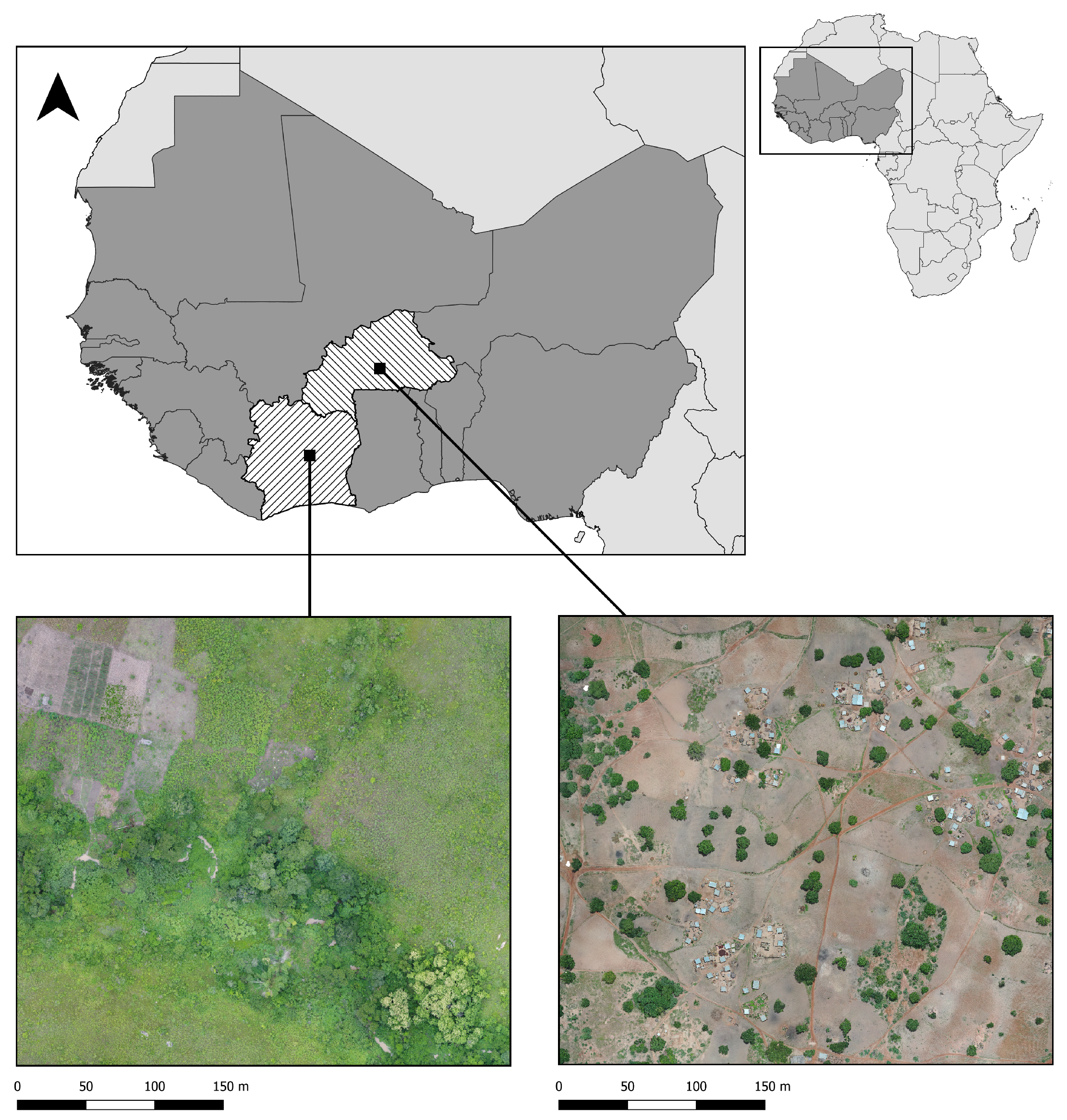
Figure 2.
Example of image labeling using QGIS.
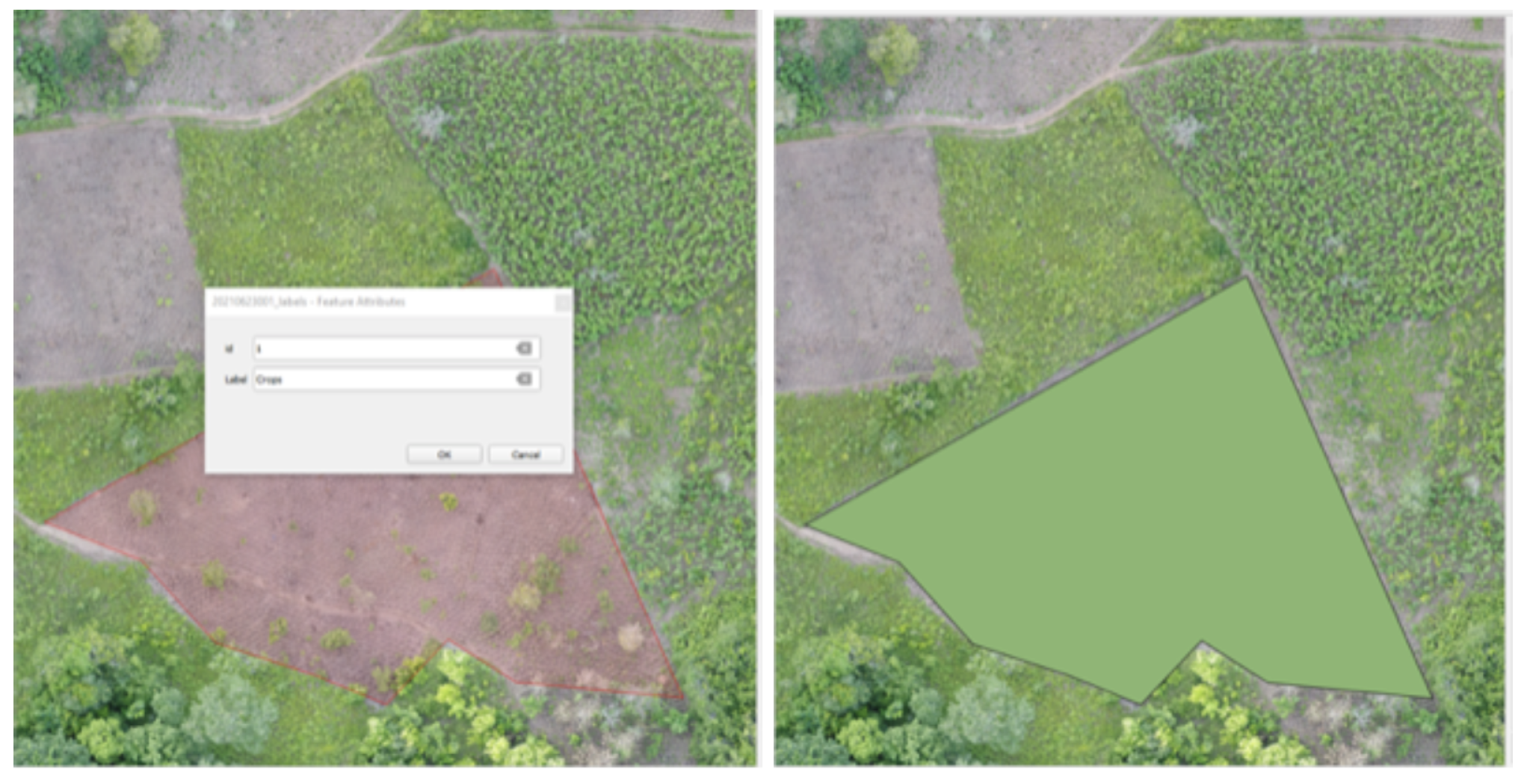
Figure 3.
Example of image labeling using GroundWork.
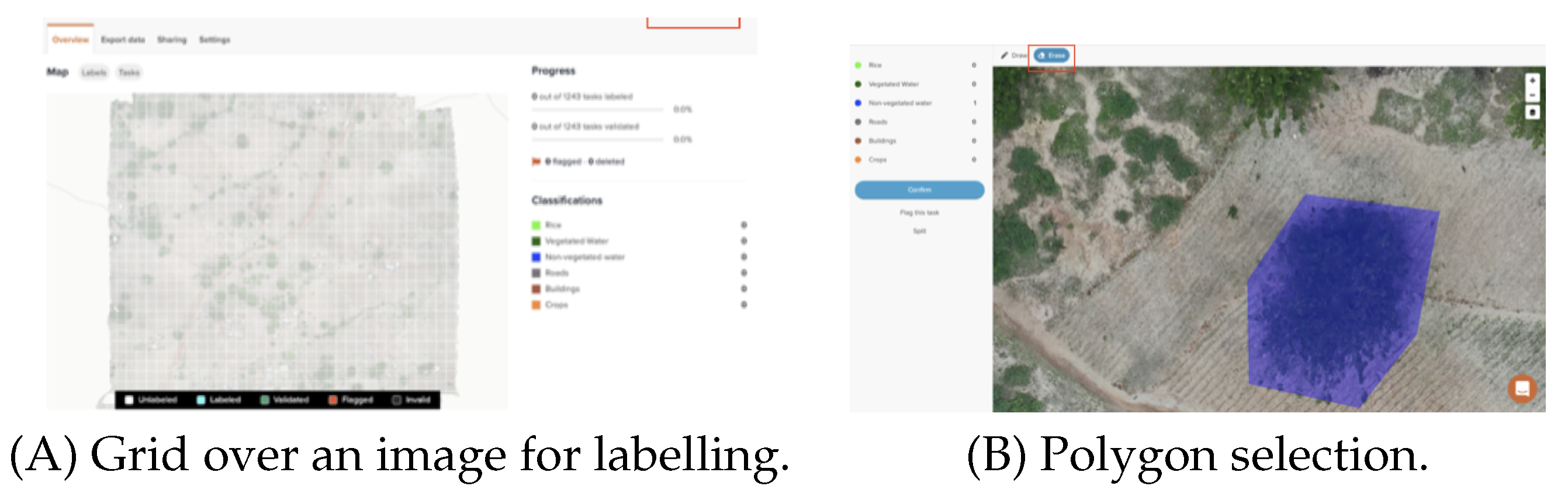
Figure 4.
Gold standard (ground-truth) masks process.

Figure 5.
Image example from Burkina Faso.
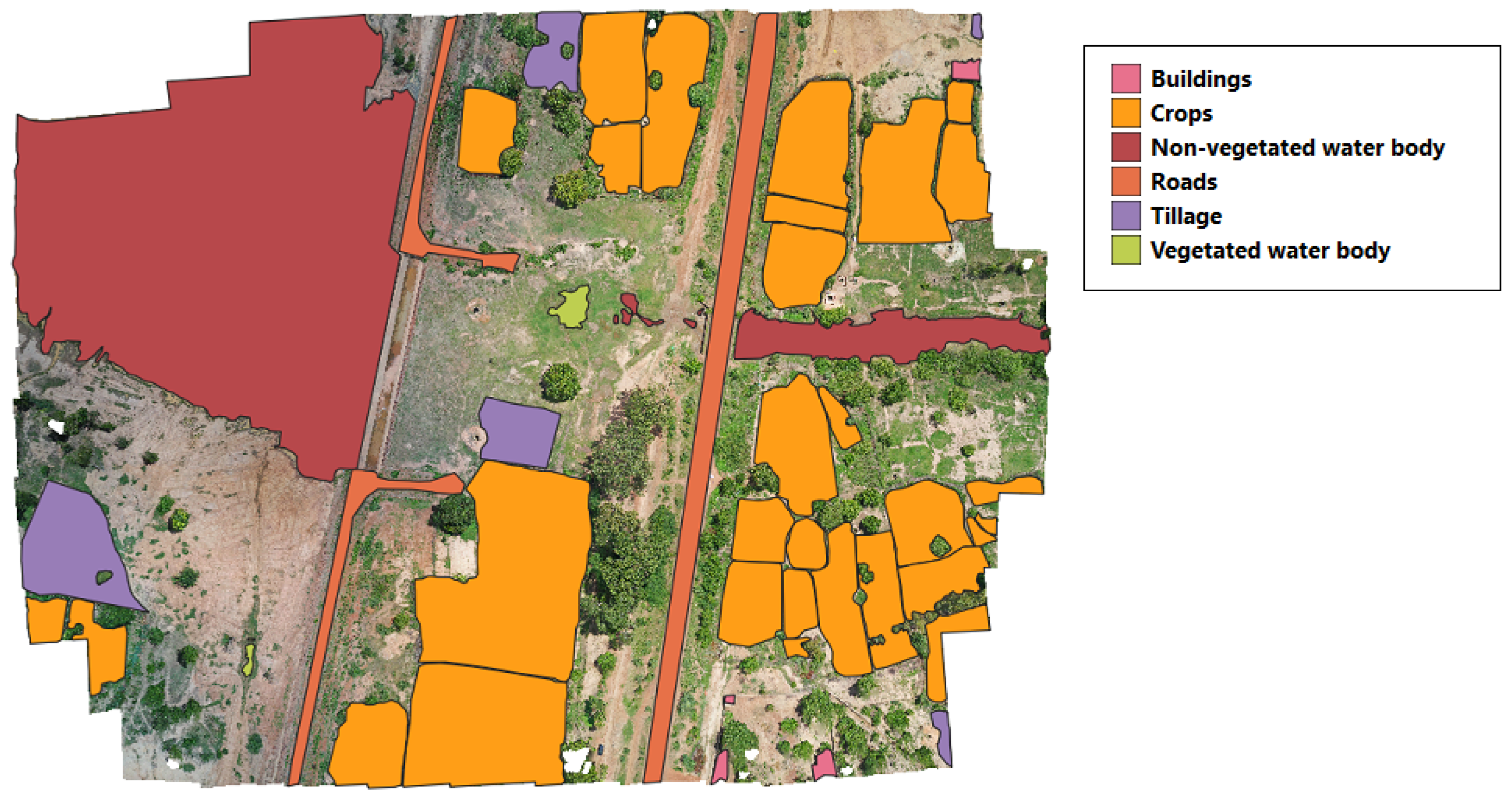
Figure 6.
Classification methodology schema.
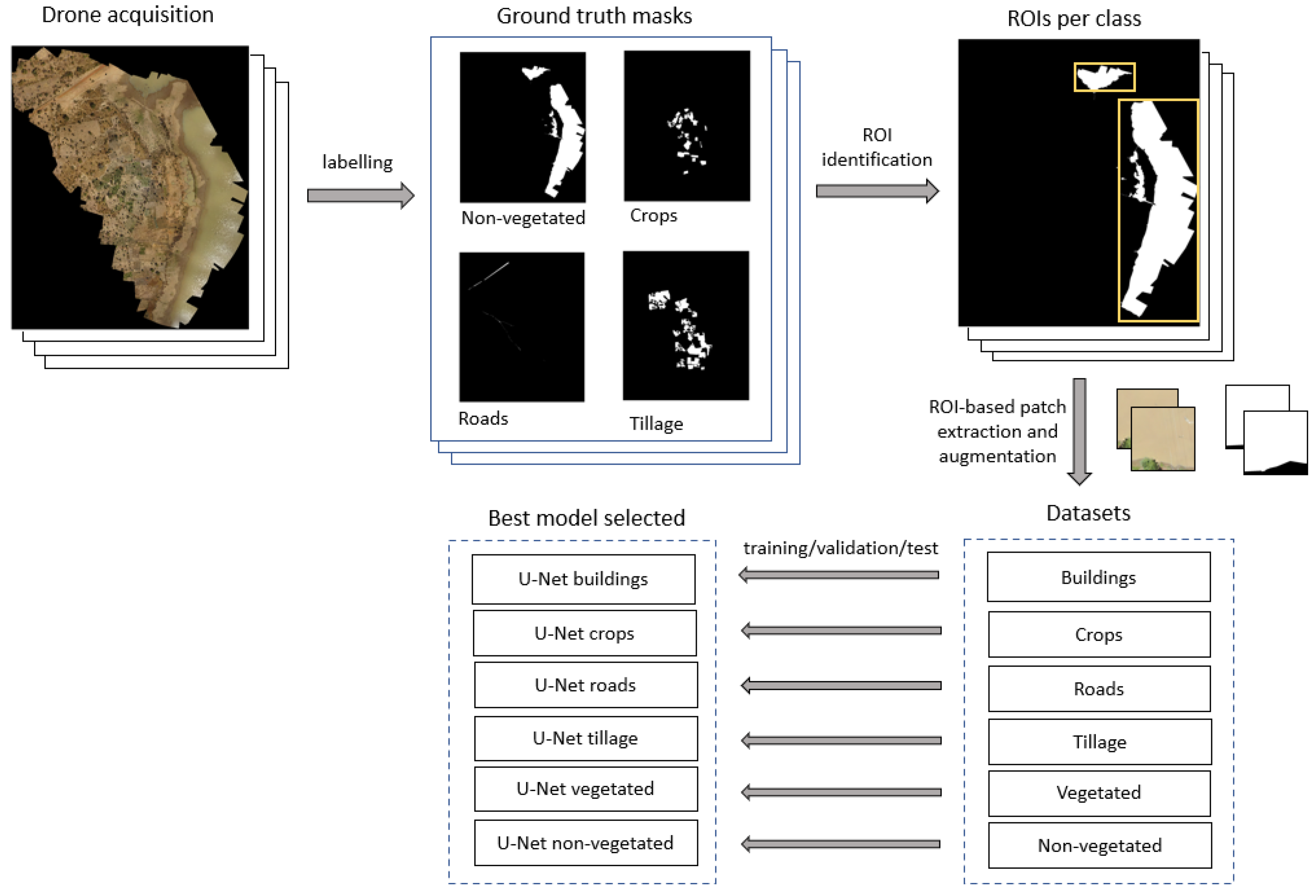
Figure 7.
Evolution of the training process using the attention U-Net architecture for patches of size 256×256 pixels. (a) Buildings. (b) Crops. (c) Non-vegetated water bodies. (d) Roads. (e) Tillage. (f) Vegetated water bodies.
Figure 7.
Evolution of the training process using the attention U-Net architecture for patches of size 256×256 pixels. (a) Buildings. (b) Crops. (c) Non-vegetated water bodies. (d) Roads. (e) Tillage. (f) Vegetated water bodies.
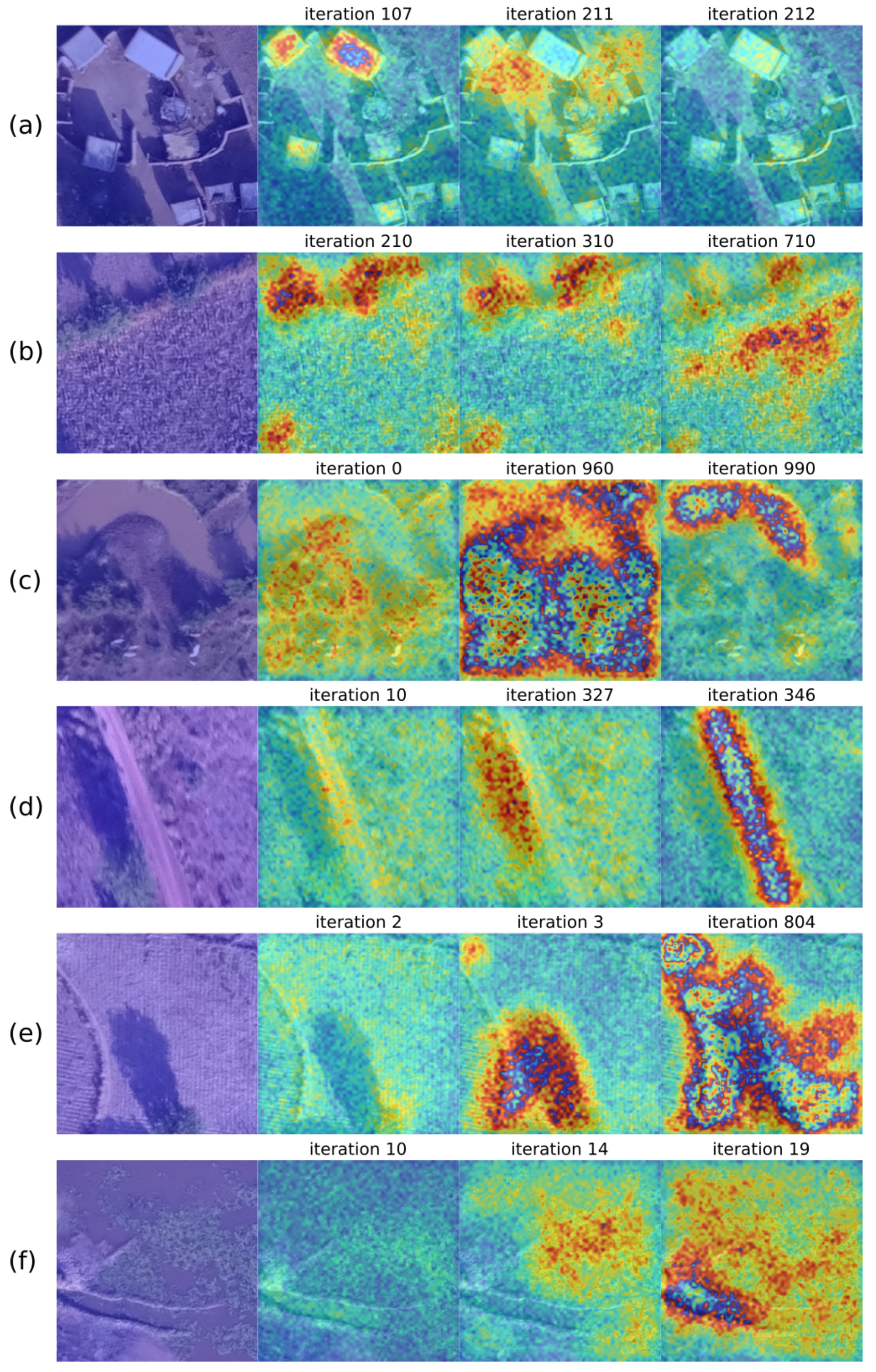
Figure 8.
Predictions using the U-Net architecture for patches of size 256×256 pixels. (a) Buildings. (b) Crops. (c) Non-vegetated water bodies. (d) Roads. (e) Tillage. (f) Vegetated water bodies.
Figure 8.
Predictions using the U-Net architecture for patches of size 256×256 pixels. (a) Buildings. (b) Crops. (c) Non-vegetated water bodies. (d) Roads. (e) Tillage. (f) Vegetated water bodies.
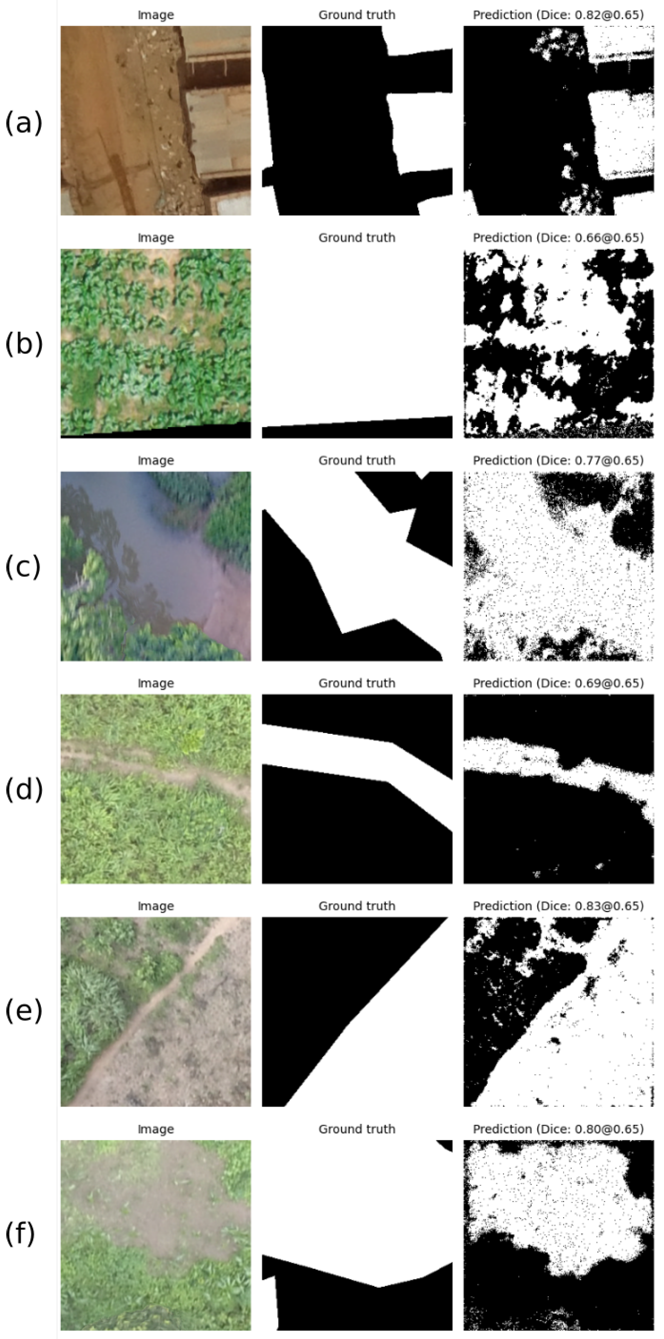
Figure 9.
Future proposal: human-supervised tool for improved drone labeling. The idea is adapted from [35,39].
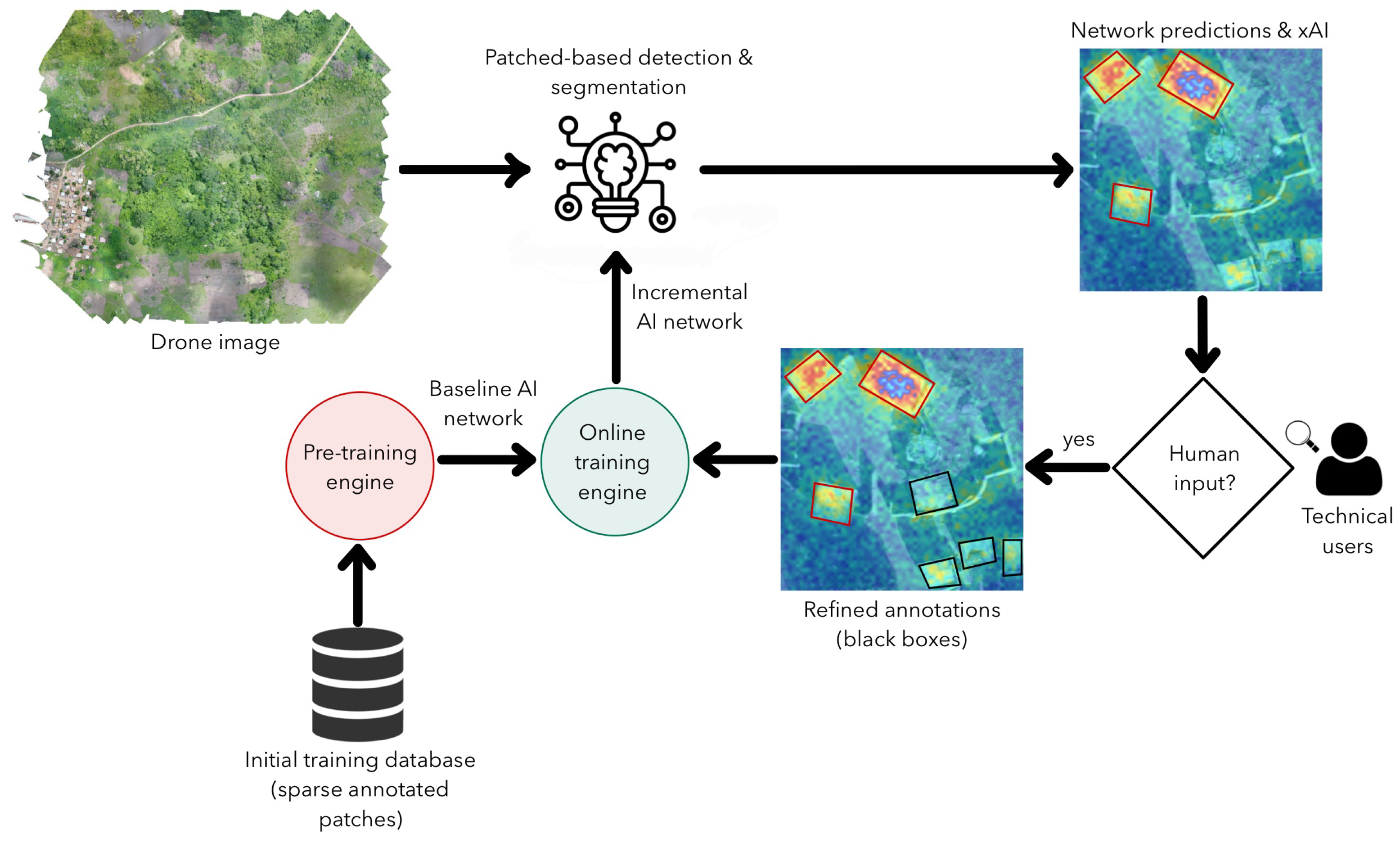

Table 1.
Number of images and patches by class for training, validation and test.
| Class | # drone images |
# train/val images |
# train/val patches | # test images |
# test patches | ||
| 256×256 | 512×512 | 256×256 | 512×512 | ||||
| Buildings | 48 | 36 | 7441 | 1324 | 12 | 4835 | 714 |
| Crops | 93 | 69 | 229522 | 58738 | 24 | 64357 | 16440 |
| Roads | 60 | 45 | 38799 | 3908 | 15 | 14330 | 2106 |
| Tillage | 42 | 31 | 86988 | 22817 | 11 | 39025 | 10264 |
| Non-vegetated | 37 | 27 | 9194 | 2232 | 10 | 79 | 1 |
| Vegetated | 20 | 15 | 4660 | 1107 | 5 | 564 | 125 |
Table 2.
Summary of the percentage of the class per patch in each category.
| Burkina Faso | ||||||||
| Patch size | 256x256 | 512x512 | ||||||
| Class | patches | min (%) | mean (%) | max (%) | patches | min (%) | mean (%) | max (%) |
| Buildings | 6584 | 10.01 | 33.72 | 100 | 778 | 20.05 | 35.81 | 87.9 |
| Crops | 14440 | 10.00 | 76.70 | 100 | 3662 | 20.00 | 71.23 | 100.0 |
| Roads | 42810 | 10.00 | 29.51 | 100 | 4513 | 20.00 | 36.72 | 100.0 |
| Tillage | 121952 | 10.00 | 75.49 | 100 | 32089 | 20.00 | 70.35 | 100.0 |
| Non-vegetated | 7734 | 10.09 | 91.73 | 100 | 1900 | 20.08 | 89.51 | 100.0 |
| Vegetated | 251 | 10.17 | 65.89 | 100 | 58 | 20.49 | 61.03 | 100.0 |
| Côte d’Ivoire | ||||||||
| Patch size | 256x256 | 512x512 | ||||||
| Class | patches | min (%) | mean (%) | max (%) | patches | min (%) | mean (%) | max (%) |
| Buildings | 5692 | 10.0 | 46.5 | 100 | 1260 | 20.0 | 35.6 | 82 |
| Crops | 279439 | 10.0 | 79.5 | 100 | 71516 | 20.0 | 74.2 | 100 |
| Roads | 10319 | 10.0 | 31.4 | 100 | 1501 | 20.0 | 26.7 | 96 |
| Tillage | 4061 | 10.0 | 69.4 | 100 | 992 | 20.1 | 62.3 | 100 |
| Non-vegetated | 1539 | 10.1 | 55.3 | 100 | 333 | 20.0 | 56.3 | 100 |
| Vegetated | 5646 | 10.0 | 62.3 | 100 | 1107 | 20.1 | 58.5 | 100 |
Table 3.
Results of the classification process using a U-Net architecture for 256x256 pixels patch size, where the best fold is reported in bold font. The results are reported in terms of cross validation (CV), false positives (FP), false negatives(FN), true negatives (TN), true positives (TP), precision, recall and dice.
| Class | CV | FP | FN | TN | TP | Precision | Recall | Dice |
| Vegetated water body | 1 | 0.17 | 0.15 | 0.15 | 0.53 | 0.75 | 0.78 | 0.68 |
| 2 | 0.25 | 0.19 | 0.20 | 0.37 | 0.59 | 0.66 | 0.56 | |
| 3 | 0.21 | 0.12 | 0.22 | 0.45 | 0.68 | 0.78 | 0.65 | |
| Avg. | 0.21 | 0.15 | 0.19 | 0.45 | 0.67 | 0.74 | 0.63 | |
| Tillage | 1 | 0.10 | 0.03 | 0.13 | 0.74 | 0.88 | 0.96 | 0.88 |
| 2 | 0.10 | 0.09 | 0.15 | 0.66 | 0.87 | 0.88 | 0.82 | |
| 3 | 0.11 | 0.05 | 0.13 | 0.71 | 0.87 | 0.93 | 0.86 | |
| Avg. | 0.10 | 0.06 | 0.14 | 0.70 | 0.87 | 0.92 | 0.85 | |
| Roads | 1 | 0.09 | 0.07 | 0.63 | 0.21 | 0.70 | 0.74 | 0.70 |
| 2 | 0.06 | 0.06 | 0.71 | 0.17 | 0.73 | 0.75 | 0.71 | |
| 3 | 0.16 | 0.15 | 0.51 | 0.17 | 0.52 | 0.53 | 0.43 | |
| Avg. | 0.10 | 0.09 | 0.62 | 0.18 | 0.65 | 0.67 | 0.61 | |
| Non-vegetated water body | 1 | 0.02 | 0.54 | 0.06 | 0.38 | 0.95 | 0.41 | 0.50 |
| 2 | 0.21 | 0.26 | 0.26 | 0.27 | 0.57 | 0.51 | 0.48 | |
| 3 | 0.22 | 0.03 | 0.18 | 0.57 | 0.72 | 0.96 | 0.75 | |
| Avg. | 0.15 | 0.28 | 0.17 | 0.41 | 0.74 | 0.63 | 0.58 | |
| Crops | 1 | 0.10 | 0.06 | 0.10 | 0.74 | 0.87 | 0.93 | 0.86 |
| 2 | 0.13 | 0.04 | 0.09 | 0.75 | 0.85 | 0.95 | 0.86 | |
| 3 | 0.09 | 0.04 | 0.10 | 0.76 | 0.89 | 0.95 | 0.88 | |
| Avg. | 0.11 | 0.05 | 0.10 | 0.75 | 0.87 | 0.94 | 0.86 | |
| Building | 1 | 0.04 | 0.07 | 0.51 | 0.38 | 0.89 | 0.84 | 0.81 |
| 2 | 0.04 | 0.08 | 0.57 | 0.31 | 0.88 | 0.80 | 0.76 | |
| 3 | 0.04 | 0.03 | 0.54 | 0.38 | 0.90 | 0.92 | 0.87 | |
| Avg. | 0.04 | 0.06 | 0.54 | 0.35 | 0.89 | 0.85 | 0.81 |
Table 4.
Results of the classification process using an attention U-Net architecture used for 256x256 pixels patch size, where the best fold is reported in bold font. The results are repported in terms of cross validation (CV), false positives (FP), false negatives(FN), true negatives (TN), true positives (TP), precision, recall, F1-score, and Dice.
| Class | CV | FP | FN | TN | TP | Precision | Recall | Dice |
|---|---|---|---|---|---|---|---|---|
| Vegetated water body | 1 | 0.27 | 0.08 | 0.15 | 0.49 | 0.64 | 0.85 | 0.67 |
| 2 | 0.28 | 0.11 | 0.17 | 0.44 | 0.61 | 0.81 | 0.64 | |
| 3 | 0.08 | 0.14 | 0.24 | 0.53 | 0.81 | 0.72 | 0.70 | |
| Avg. | 0.21 | 0.11 | 0.19 | 0.49 | 0.69 | 0.79 | 0.67 | |
| Tillage | 1 | 0.06 | 0.25 | 0.18 | 0.51 | 0.85 | 0.66 | 0.67 |
| 2 | 0.11 | 0.23 | 0.13 | 0.53 | 0.80 | 0.68 | 0.69 | |
| 3 | 0.03 | 0.55 | 0.27 | 0.15 | 0.77 | 0.20 | 0.27 | |
| Avg. | 0.07 | 0.34 | 0.19 | 0.40 | 0.81 | 0.51 | 0.54 | |
| Roads | 1 | 0.15 | 0.12 | 0.53 | 0.20 | 0.70 | 0.67 | 0.58 |
| 2 | 0.15 | 0.10 | 0.48 | 0.27 | 0.71 | 0.69 | 0.60 | |
| 3 | 0.35 | 0.06 | 0.40 | 0.19 | 0.51 | 0.77 | 0.46 | |
| Avg. | 0.22 | 0.09 | 0.47 | 0.22 | 0.64 | 0.71 | 0.55 | |
| Non-vegetated water body | 1 | 0.10 | 0.58 | 0.30 | 0.02 | 0.36 | 0.03 | 0.04 |
| 2 | 0.06 | 0.10 | 0.02 | 0.82 | 0.91 | 0.88 | 0.85 | |
| 3 | 0.20 | 0.05 | 0.26 | 0.49 | 0.71 | 0.90 | 0.72 | |
| Avg. | 0.12 | 0.24 | 0.19 | 0.44 | 0.66 | 0.60 | 0.54 | |
| Crops | 1 | 0.07 | 0.17 | 0.14 | 0.62 | 0.85 | 0.76 | 0.75 |
| 2 | 0.04 | 0.27 | 0.13 | 0.55 | 0.89 | 0.66 | 0.72 | |
| 3 | 0.16 | 0.04 | 0.05 | 0.75 | 0.81 | 0.94 | 0.84 | |
| Avg. | 0.09 | 0.16 | 0.11 | 0.64 | 0.85 | 0.79 | 0.77 | |
| Building | 1 | 0.03 | 0.06 | 0.56 | 0.36 | 0.91 | 0.84 | 0.85 |
| 2 | 0.03 | 0.07 | 0.53 | 0.37 | 0.91 | 0.82 | 0.83 | |
| 3 | 0.21 | 0.06 | 0.41 | 0.32 | 0.65 | 0.83 | 0.66 | |
| Avg. | 0.09 | 0.06 | 0.50 | 0.35 | 0.82 | 0.83 | 0.78 |
Disclaimer/Publisher’s Note: The statements, opinions and data contained in all publications are solely those of the individual author(s) and contributor(s) and not of MDPI and/or the editor(s). MDPI and/or the editor(s) disclaim responsibility for any injury to people or property resulting from any ideas, methods, instructions or products referred to in the content. |
© 2023 by the authors. Licensee MDPI, Basel, Switzerland. This article is an open access article distributed under the terms and conditions of the Creative Commons Attribution (CC BY) license (http://creativecommons.org/licenses/by/4.0/).
Copyright: This open access article is published under a Creative Commons CC BY 4.0 license, which permit the free download, distribution, and reuse, provided that the author and preprint are cited in any reuse.
supplementary.zip (1.70MB )
Submitted:
24 March 2023
Posted:
28 March 2023
You are already at the latest version
Alerts
A peer-reviewed article of this preprint also exists.
supplementary.zip (1.70MB )
This version is not peer-reviewed
Submitted:
24 March 2023
Posted:
28 March 2023
You are already at the latest version
Alerts
Abstract
Disease control programs need to identify breeding sites of mosquitoes which transmit malaria and other diseases to target interventions and identify environmental risk factors. Increasing availability of very high resolution drone data provides new opportunities to find and characterize these vector breeding sites. Within this study, we identified land cover types associated with malaria vector breeding sites in West Africa. Drone images from two malaria endemic regions in Burkina Faso and Côte d’Ivoire were assembled and labeled using open-source tools. We developed and applied a workflow using region of interest-based and deep learning methods to classify these habitat types from very high resolution natural color imagery. Analysis methods achieved a dice coefficient ranging between 0.68 and 0.88 for different vector habitat types; however, this classifier consistently identified the presence of specific habitat types of interest. This establishes a framework for developing deep learning approaches to identify vector breeding sites and highlights the need to evaluate how results will be used by control programs.
Keywords:
Subject: Computer Science and Mathematics - Artificial Intelligence and Machine Learning
1. Introduction
Land-use changes, such as agricultural expansion, can create new aquatic habitats suitable for breeding sites for mosquito vectors that transmit malaria and other diseases [1]. When aquatic mosquito habitats can be identified, disease control programs can implement targeted interventions such as larval source management, reducing mosquito densities through chemical, biological, or environmental means [2]. While traditional approaches relied on ground-based surveys, Earth Observation (EO) data, such as drone and satellite data, is increasingly utilized to identify potential breeding sites rapidly and target control measures [3,4,5,6,7]. EO data additionally provides new opportunities to characterize mosquito habitats and monitor changes in these habitats in response to environmental change [8].
Obtaining actionable information from EO data requires classifying imagery into relevant habitat types. The specific classes of interest are highly dependent on local vector ecology; for example, Anopheles funestus, the second most important malaria vector in Africa, commonly breeds in large, vegetated water bodies [9,10,11,12]. In contrast, An. gambiae breed in small or temporary, often man-made water bodies across a wide range of habitat types, including roads, agricultural irrigation such as rice paddies, sunlit rivers and streams, and quarries or construction sites [2,13,14]. Additionally, the type of information required when classifying EO data depends on the end-use. While a vector control program may benefit from knowing the probability of a large area containing habitat types, ecological and epidemiological studies may require more detailed segmentation approaches to characterize the shape and configuration of different habitat types [15,16,17,18,19,20,21].
For these applications, it is critical that EO data is collected simultaneously as ground-based vector surveys or is recent enough to provide actionable information for control programs. This has led to increased use of EO data with high spatial and temporal resolutions, such as user-defined imagery collected by drone (unmanned aerial vehicles or UAVs) or daily commercial satellite data (e.g., Planet). These data typically have a low spectral resolution, limiting the utility of traditional pixel-based approaches requiring data measured outside the visible spectrum [22,23]. Alternatively, deep learning approaches, such as convolutional neural networks (CNNs), have revolutionized image analysis by efficiently analyzing image textures, patterns, and spectral characteristics using self-learning artificial intelligence approaches to identify features in complex environments [20,24,25,26].
Multiple approaches have been applied for identifying habitats and their characteristics from EO imagery for operational use by vector-borne disease control programs. In Malawi, Stanton et al. [7] assessed approaches for identifying the aquatic habitats of larval-stage malaria mosquitoes. They assessed geographical object-based image analysis (GeoOBIA), a method that groups contiguous pixels into objects based on prespecified pixel characteristics. The objects were classified by a random forest supervised classification and demonstrated strong agreement with test samples, successfully identifying larval habitat characteristics with a median accuracy of 98%. Liu et al. [27] developed a framework for mapping the spatial distribution of suitable aquatic habitats for the snail hosts of the debilitating parasitic disease Schistosomiasis along the Senegalese River Basin. A deep learning U-Net model was built to analyze high-resolution satellite imagery and to produce segmentation maps of aquatic vegetation. The model produced predictions of snail habitats with higher accuracy than commonly used pixel-based classification methods such as random forest. Hardy et al. [28] developed a novel approach to classify and extract malaria vector larval habitats from drone imagery in Zanzibar, Tanzania. This used computer vision to assist manual digitization. This approach was found to significantly outperform supervised classification approaches, which were unsuitable for mapping potential vector larval habitats in the study region based on accuracy scores.
For other applications, a range of analysis approaches has been developed to identify features from drone imagery [29]. For example, gray-level co-occurrence matrix (GLCM) techniques for vegetation structure modeling have been applied to reduce noise and improve the classification of UAV images by using textural information [29]. Similarly, Hu et al. [30] proposed a two-step approach coupling classification and regression trees to estimate the ground coverage of wheat crops from UAV imagery with coarse spatial resolutions. First, a classification tree-based per-pixel segmentation was applied to segment fine-resolution reference images into binary reference images of vegetated and non-vegetated areas. Next, a regression-tree-based model was used to develop sub-pixel classification methods. This two-step approach increased classification accuracy on both real and synthetic image datasets. Other studies have explored the utility of using spectral data to monitor land cover changes using very high-resolution imagery. For example, Komarkova et al. [31] calculated eight vegetation indices calculated from red, green, and blue (RGB) UAV imagery with a 1.7 cm per pixel resolution; indices were identified, which allowed the identification of vegetated and clear water surfaces. This high-resolution RGB data can also be integrated with satellite imagery with higher spectral resolution and lower spatial resolution. For example, Cao et al. [32] applied a multiple criteria spectral mixture analysis (MCSMA) to map fractional urban land covers (vegetation, impervious surface, and soil) on Landsat-8 surface reflectance imagery (30 m/pixel, seven optical bands) with high-resolution RGB data from Google Earth using a multistep process. First, the authors obtain spectrally pure patches through minimum distance, maximum likelihood, and support vector machine classifiers. Mixed pixels at boundary regions of the patches were removed by applying the morphological erosion operation, and the centroid of each patch was computed to form end member candidates. Then, the MCSMA constructs all possible end member models using a spatially adaptive strategy. All possible end member models were finally tested for the target pixel using a constrained linear spectral unmixing method to improve classification accuracy. Rustowicz et al. [33] compare the performance between a 3D U-Net with a 3x3 kernel followed by batch norm and a leaky Rectified Linear Unit (ReLU) activation and well-known models incorporating both CNNs and recurrent neural networks (RNN) for semantic segmentation of multi-temporal, multi-spatial satellite images. Sentinel 1, Sentinel 2, and Planet satellite imagery of sparse ground truth labels of crop fields in South Sudan and northern Ghana were used in this contribution. In addition, a German dataset was used in the comparison. Ground truth labels consist of geo-referenced polygons, where each polygon represents an agricultural field boundary with a crop type label, including maize, groundnut, rice, and soya bean. As a part of the experimental process, the authors performed a hyperparameter search across optimization methods through Adam and SGD techniques. The authors find that models trained on the German dataset outperformed models tested on South Sudan and Ghana datasets. Smaller training sets, high cloud cover, and complex landscapes in the smallholder setting affected the results obtained.
Building on these methods, we aimed to develop and validate deep learning approaches to identify land classes associated with the breeding sites of malaria mosquito vectors in West Africa. Data were assembled from multiple sites in Burkina Faso and Côte d’Ivoire to develop an approach able to generalize to different malaria-endemic landscapes. We used RGB drone images from the study sites to build a training dataset and to implement two CNN-based frameworks using the U-Net and attention U-Net architectures to identify features of interest for Anopheles breeding ecology. The specific objectives of this study were to (i) collect and assemble a dataset of drone images in malaria-endemic areas in Côte d’Ivoire and Burkina Faso; (ii) develop the protocol to label land classes of interest in drone imagery; (iii) assemble a labeled dataset for each class and (iv) train, validate and test U-net and attention U-net deep learning architectures. Final algorithms were assessed based on the performance of predicting the presence of the classes of interest in test images using the best model after cross validation.
2. Materials and Methods
2.1. Drone mapping
Drone surveys were conducted in two malaria endemic sites in West Africa: Saponé, Burkina Faso and Bouaké, Côte d’Ivoire where the incidence of malaria (per 1000 population at risk) are 389.9 and 2871, respectively. Both sites are rural with extensive small-scale agriculture and highly seasonal rainfall and malaria transmission patterns. Saponé is located 45 km south-west of Ouagadougou, Burkina Faso and has reported extremely high malaria prevalence of predominantly Plasmodium falciparum [34]. The main malaria in this site is An. gambiae s.l., with low densities of other species also reported. Between November 2018 - November 2019, fixed wing (Sensefly eBee) and quadcopter (DJI Phantom 4 Pro) drones were used to collect RGB data at 2-10cm per pixel resolution. Similarly, in Bouaké, we conducted targeted drone surveys from June - August 2021 using a DJI Phantom 4 Pro drone to collect RGB data at a 2cm per pixel resolution as described by [6]. This area was also rural and dominated by small scale agriculture; however, this site had different vector compositions, including high densities of An. funestus. For both sites, drone images were processed using Agisoft Metashape Professional2 to generate orthomosaics. The drone images cover 11.52 km2 and 30.42 km2 area for Burkina Faso and Côte d’Ivoire, as illustrated in Figure 1. Both sites were dominated by agriculture, mainly yams, cassava, cashew, peanuts, and maize.
2.2. Image Labeling and Development of Labeled Dataset
We identified specific land cover classes of interest associated with Anopheles breeding sites, including water bodies and irrigated agricultural land types [6]. We differentiated between vegetated and non-vegetated water bodies as An. funestus is most commonly identified only in vegetated water bodies. We additionally identified habitat types not associated with Anopheles breeding sites but with human activities, including roads and buildings. The final land cover classes of interest for this analysis included vegetated and non-vegetated water bodies, irrigated crops (planted vegetation with no tree cover), tillage (land cleared for planting crops), buildings and roads. While this classification cannot specifically identify whether or not an area is an Anopheles breeding site, this provides the basis for targeting future entomological surveys and wider epidemiological studies on how landscape impacts malaria transmission.
To identify these classes using a supervised deep learning approach, we first needed to assemble a dataset of harmonised labelled images. We manually labelled all drone acquisitions to generate gold standard (i.e., labeled images) masks for each of the specific land classes. Trained personnel familiar with the study area validated the labels. This process was performed using two different tools: QGIS3 and GroundWork4. The former is a Geographic Information System (GIS) open-source desktop application that allows inputting geo-referenced images and annotating manually using polygons (Figure 2). Groundwork, on the other hand, is a cloud-based licensed tool where the images are uploaded for labelling. In this cloud-based interface, a grid is overlaid in the image as illustrated in Figure 3A. The user is then able to select one of the predefined classes to assign the corresponding class over the images as shown in Figure 3B. While this tool has a streamlined workflow to facilitate labelling, this required internet access, had a limited data allowance and was not suitable in all contexts. The obtained polygons from both tools were checked to detect invalid polygons and were corrected manually.
Once all the images were labeled, ground-truth masks were created for the supervised image classification. As shown in Figure 4, first, we create a subset of vector layers, one for each class. Then, we rasterized the vector layers to create a separate raster image for each class. The land class presence depended on the acquisition site’s characteristics. For example, Figure 5 shows a labeled region from Burkina Faso where all the land classes are present; however, this is not the case for all the images. Images that did not contain labeled polygons were not considered in this study.
We built six land class datasets: crops, tillage, roads, buildings, vegetated water bodies and non-vegetated water bodies (defined at the beginning of this section). For each dataset, we selected only the drone images that contained labels of the corresponding land class. From each dataset we randomly selected images for training, validation and test. To avoid bias related to the training data, we considered using a 3-fold cross-validation scheme.
Due to GPU memory constrains, the entire drone image and its corresponding labels were split into several patches, which were used to train, validate and test the deep learning models. In addition, because of the variable extension of each labeled polygon, splitting the image in a grid pattern resulted in a highly unbalanced dataset where the background predominated over the class of interest. Instead, we used a new approach for data patching and augmentation based on ROI-shifting, described in [35], to avoid this imbalance. This method also prevented potential bias caused by the network focusing on the background instead of the class of each patch. The augmentation aimed to train the models robustly in the presence of variable neighborhood context information. Thus, we identified the ROIs and frame them in rectangles, which could contain one or more polygons as illustrated in Figure 6. Patches of sizes 256×256 and 512×512 pixels were extracted from those rectangles and assigned to each training, validating and testing datasets. A summary of the number of images and patches in each dataset is reported in Table 1. For each patch size, we report in Table 2 the average percentage of the class present in the dataset. This is computed, per patch, as the ratio of the pixels belonging to each class and the background pixels. Patches with classes representing less than 10% (256×256) or 20% (512×512) of the patch size were eliminated from the datasets. The total number of patches obtained for each class differs by study site; while Burkina Faso contained more tillage areas, Côte d’Ivoire had more irrigated crops. Considering both sites, water body datasets contained the least number of patches. On average, non-vegetated water bodies, tillage, and crops covered greater percentages of patches as these classes were more likely to be larger.
2.3. Algorithm Development
We developed a multi-step approach to classifying multiple land classes from patches, as shown in Figure 6. Following the dataset preparation, two deep learning segmentation models were selected: U-net and attention U-Net. The U-Net is a widely used architecture for semantic segmentation tasks. This method relies on the upsampling technique, which increases an image’s dimension (i.e., the number of rows and/or columns). Thus, the present method builds on a conventional network with successive layers by using upsampling operators to replace pooling operations, which implies using contraction and expansion paths (i.e., encoder and decoder respectively). The contraction part reduces the spatial dimensions in every layer and increases the channels. Meanwhile, the expansive part increases the spatial dimensions while reducing the channels. Finally, using also skip connections between the encoder and decoder, the spatial dimensions are restored to predict each pixel in the input image. An important modification in the U-Net is that many feature bands are in the upper sampling part, allowing the network to propagate context information to higher-resolution layers. Consequently, the expanding trajectory is more or less symmetric to the contracted part and produces a U-shaped architecture [36]. Attention U-Net adds a self-attention gating module in every skip connection of the U-Net architecture without increasing computation overhead. These modules are incorporated to improve sensitivity, accuracy, and add visual explanability to the network. The improvement is performed by focusing on the features of the regions of interest rather than the background [37,38].
Regarding the computational features used in this study, data preparation and deep learning experiments were executed on an 8-core Intel(R) Xeon E5-2686 @ 2.3 GHz CPU with 60 GiB RAM and one 16 GiB RAM Nvidia Tesla V100 GPU on Amazon Elastic Compute Cloud service (AWS).
2.4. Evaluation metrics
To quantitatively assess the similarities between the predicted and gold standard object areas, we used the dice coefficient. This divides two times the area of overlap by the total number of pixels in both images, as shown in Equation 1.
The dice coefficient takes values from 0 to 1, in which 1 represents a complete match between the ground-truth and the prediction. We additionally calculated the precision and recall metrics which are computed based on true positives (TP), false positives (FP), true negatives (TN), and false negatives (FN) as described in equations 2, and 3 respectively.
Based on the aforementioned elements, we performed different experiments that are described in the following section.
3. Results
As the number of ROIs in every drone image was not the same, the number of patches (generated from the ROIs) in each fold varied from class to class. As a result, we used up to 90% of the CPU RAM capacity in the experiments containing the higher number of patches. This computational load was due to caching the data and annotations in CPU RAM prior to moving the batches to the GPU RAM in the training, validation, and test phases. This approach reduces the number of CPU-GPU data transfers which can intensively impact the training time. The average training and cross-validation time was approximately 12 hours.
The U-Net and attention U-Net architectures were used to classify the different classes organized in sets of patches of 256×256 and 512×512 pixels in size using a 3-fold cross-validation procedure. Table 3 shows the results for the U-Net using patches with a size of 256×256 pixels. For vegetated water bodies, one of our primary classes of interest, the model reached its highest dice score at 0.68 in the first fold and an average of 0.63. Non-vegetated water bodies had a higher dice score of 0.75 and 0.58 on average, showing the worst performance among all the classes. Crops, tillage, and buildings had the best overall performance, above 0.80 in all validation sets, followed by roads that reached 0.71. The same U-Net architecture was also trained with patches of 512x512 pixels in size. For both training approaches, all classes achieved comparable results; however, the model trained with 256x256 pixel size patches outperformed, on average, the 512×512 model in every class. The detailed table showing the performance of the 512×512 pixels size model is in the Supplementary Information.
Similarly to the U-Net experiments, we trained the attention U-Net with patches of 256x256 pixels. The evolution of the training is shown in Figure 7. The areas where the network finds relevant features for segmentation are displayed in red, while the blue areas correspond to less essential regions. The first column shows the original patch, and the following columns are the heatmaps according to an iteration number indicated above; however, they correspond to different epochs. In general, for non-vegetated water body (Figure 7c), roads (Figure 7d), and vegetated water body (Figure 7f) patches, we notice that, as the number of iterations increases, the network focuses more on the areas of interest for learning. Nevertheless, in the case of buildings (Figure 7a), the initial iteration focuses more on the construction than the final one because it corresponds to a different epoch and batch, meaning that iteration 212 corresponds to an early epoch where the network is not fully updated or a batch with different data distribution than the patch analyzed. Another important highlight is that in some iterations, the network concentrates not on the class but in the shadows of the patch, such as in Figure 7d iteration 327 and Figure 7d iteration 3.
The quantitative results to evaluate the performance of the attention U-Net using patches of 256×256 pixels are reported in Table 4. Comparing these results with the ones obtained with the 256×256 U-Net model, we observe that the vegetated and non-vegetated water body classes have improved performance. Despite that, the first fold of the non-vegetated water body class showed a low dice performance (below 5%), meaning the training is unstable across the 3 folds and may impact the inference process due to different data distributions present in the datasets. Therefore, cross-validation provided insights into the robustness and stability of the trained models.
We also trained the attention U-Net using patches of 512×512 pixels. However, we used a subset of patches per class ranging from 5% to 20% to test the model performance on the vegetated and non-vegetated water bodies, crops, and buildings classes. Even though it shows an improvement in the water body classes compared to the 256×256 pixels U-Net model using the best fold as a reference, the standard deviation calculated after the cross-validation is higher, meaning the network is not entirely stable. For instance, in the non-vegetated class, the dice score ranges from 0.1 to 0.91 in the attention U-Net 512×512 pixels model. We reported all results for this last experiment in the Supplementary Information.
We selected the U-Net 256×256 pixels model to evaluate the predicted maks as it was the most stable and robust network. Figure 8 shows the inference results for one sample patch (taken from the test dataset) per class. The first column shows the original test patch. The second column shows the gold standard in white and the background in black, whereas the third column is the network prediction, where each pixel is depicted in white if it belongs to the corresponding class with a probability higher than 0.65. The patch’s dice score is reported above each predicted mask.Figure 8a shows the buildings accurately distinguished over the soil region. In contrast, qualitative results for crop class in Figure 8b show that the network predicts as crops more regions of soil between the leaves rather than the actual crop. This may be explained due to the imprecise annotations (i.e., mask almost covering 100% of the patch area) seen in the gold standard. Figure 8c presents a water body’s segmentation despite the shadows and blurriness of the patch. Figure 8d, a show a road and a vegetated water body, respectively. In both cases, the network outperformed the manual annotation qualitatively. Finally, the tillage model output shown in Figure 8e predicts not only the corresponding class but also areas of soil that were not prepared for cultivation.
4. Discussion
This study highlights the utility of deep learning approaches to identify potential mosquito habitats using high-resolution RGB imagery. We developed a workflow and methodology to assemble and process labeled training data to implement deep learning algorithms to automatically detect malaria vectors’ potential habitats. Although performance, as measured by the dice coefficient, was low for some classes, the classifier did consistently detect the presence of specific classes within drone imagery. In fact, we identified that the relevant information for the end-user needs, in this case, is to advertise the presence of a particular type of land cover rather than the boundary delimitation of the class. Overall, this work establishes a framework to apply artificial intelligence tools to support vector-borne disease control.
Our proposed methodology builds on a growing literature using deep learning approaches and remote sensing data to identify priority areas for implementing disease control measures. Compared to other studies using deep learning algorithms with multispectral satellite imagery to detect vector habitats, our study had lower predictive power [27], most likely due to the limited information in RGB images. In addition, the annotation process (i.e., manual labeling) is a factor we need to consider. For example, in Figure 8f, although the labeled image used for training did not encompass the entire water body boundaries, our method could find the correct pixels belonging to this class. The qualitative differences in the manual and predicted labels result in a lower dice score. Rather than relying solely on manual annotations, which can be imprecise, unsupervised learning approaches or region-growing approaches may result in more accurate ground-truth and higher-performing models [28].
In Figure 8f, our proposal using the U-Net architecture achieved better qualitative results when segmenting certain classes. In order to understand deeply where the network was focusing its attention when dealing with this task, we use the attention U-Net architecture. The results provided a clear view of which pixels were being used in the segmentation process. This introduced a level of visual interpretability of the training process and allowed us to propose a methodology to leverage the attention maps to refine manual annotations.
This tool can be improved in the future by including human supervision as proposed in Figure 9. Initially, we need a set of manually annotated patches extracted from several drone images used in the pre-training engine. The model obtained after this process could be used to segment and detect structures in a new drone image. The network will output its predictions as attention maps (heat maps with pixel probabilities). A user will then evaluate the predictions and determine if there are missing objects or if the boundaries of the detected objects are correctly segmented. These new annotations will then be used as inputs to an online training engine, improving the knowledge of the original deep learning model. This procedure should reduce the imprecision of manual annotations and allow the model to learn incrementally from new samples introduced by different users. In addition, the feedback loop should also help when there are similar qualitative characteristics (imaging features) in different class patches: a challenging process regarding data cleaning procedures.
We could also observe a difference in performance using different patch sizes. Ideally, larger patches allow the network to extract information from the object’s surroundings and identify the borders of the objects detected, such as the buildings. However, this additional information may need to be clarified in some cases. A deeper analysis, including multiresolution deep learning models, could provide a better understanding of the features needed for better segmentation of the classes proposed in this study.
Deep learning approaches based on open-access satellite data can provide a more efficient and cost-effective means for vector control programmes to identify priority areas for field surveys and targeted interventions. Larval source management is an important component in the toolkit for controlling mosquito-borne diseases, particularly in endemic contexts with persistent insecticide resistance ; however, identifying aquatic breeding sites is both time and resource intensive and can be biased by reliance on prior knowledge, convenience or assumptions. We found that the presence of specific habitat classes could be consistently detected within drone imagery. By delineating certain areas within a large, gridded landscape with a high probability of containing potential vector breeding habitat, deep learning algorithms could facilitate more targeted planning and implementation of larviciding activities. For example, vector control programmes can use this to focus finite resources on narrower areas for entomological field-based surveys or anticipate the scale of larvicide requirements for a given area. Importantly, this approach is generalisable and could be used in a range of vector-borne disease endemic contexts to identify the presence of habitats of interest that are relevant to local land cover and local vector ecology.
Additionally, this highlights the importance of identifying how the classified information will be used. While we assessed model performance using the dice coefficient, these metrics describe pixel-level classification accuracy. In some cases, this may be appropriate, such as when a epidemiological study needs to identify the precise outline of a water body. However, in many cases, these scores do not reflect the utility of the classifier. For example, a control program may only need to know where a potential breeding site is located and the relative size to plan larviciding activities.
This study also has several important limitations. While we used data from multiple sites in West Africa, these do not indicate the full range of habitats within this region or seasonal changes. Future studies could integrate data from other sources to develop more representative datasets. Additionally, limited amounts of ground-truthed data were available from these study sites, and there was insufficient data on larvae presence or absence to predict whether specific land classes contained Anopheles larvae. If data were available, this framework could be extended to predict presence or absence of specific species.
Despite these limitations, this study develops a methodology to automatically detect potential mosquito breeding sites. Although data labelling is highly labor intensive, this classifier can rapidly analyze RGB drone images collected using small, low-cost drones. Similarly, as deep learning methods are self-learning, additional datasets will likely improve the performance and applicability of these methods. Future work could develop more user-friendly interfaces to support the uptake of these methods. Together, this study sets out a useful framework to apply deep learning approaches to RGB drone imagery.
5. Conclusions
This study proposes a methodology to automatically spotlight high-resolution RGB drone images of the West Africa land cover to detect malaria vectors’ potential habitats. After a manual image annotation, images were cut in patches of size 256×256 and 512×512 pixels. Later, U-Net-based and attention U-Net-based algorithms were applied to automatically identify buildings, roads, water bodies, crops, and tillage. Finally, the best model was selected from the different experiments performed based on the dice score. Even though we have obtained promising results in identifying buildings, roads, and water bodies, crops and tillage still represent a challenge, which will be explored in future work. Nevertheless, we have demonstrated that our proposal is pertinent for helping experts to create tools to avoid the proliferation of mosquito breeding sites.
Author Contributions
Fedra Trujillano and Gabriel Jimenez contributed equally as first authors. Conceptualization, I. B., J. L., K. F. and G. C.; data curation, F. T., G. J., K. C., N. A, P. K., W. O., A. T. and M. G.; funding acquisition, I. B. and K. F.; investigation, I. B., G. C. and K. F.; methodology, F. T., G. J., M. N., K. C., E. M. and H. A.; project administration, I. B., G. C. and K. F.; resources, I. B., G. C. and K. F.; software, F. T. and G. J.; supervision, I. B., J. L. G. C. and K. F.; validation, F. T., G. J., M. N. and H. A.; visualization, F.T., G.J., M. N. and E. J.; writing—original draft preparation, F. T., G. J., M. N., I. B., K. F. and H. A.; writing—review and editing, I. B. and K. F., G. C.. All authors have read and agreed to the published version of the manuscript.
Data Availability Statement
For reproducibility purposes, the python code is available at https://github.com/healthinnovation/aerial-image-analysis.
Acknowledgments
This work was supported by a Sir Henry Dale fellowship awarded to KMF and jointly funded by the Wellcome Trust and Royal Society (Grant no 221963/Z/20/Z). Additional funding was provided by the BBSRC and EPSRC Impact Accelerator Accounts (BB/X511110/1) and the CGIAR Research Program on Agriculture for Nutrition and Health (A4NH). K.C. and J.L. are also partly supported by the UK aid from the UK government (Foreign, Commonwealth & Development Office-funded RAFT [Resilience Against Future Threats] Research Programme Consortium). The views expressed do not necessarily reflect the UK government’s official policies nor the opinions of A4NH or CGIAR.
Conflicts of Interest
The authors declare no conflict of interest. The funders had no role in the design of the study; in the collection, analyses, or interpretation of data; in the writing of the manuscript, or in the decision to publish the results.
Abbreviations
The following abbreviations are used in this manuscript:
| EO | Earth Observation |
| UAV | unmanned aerial vehicle |
| CNN | convolutional neural networks |
| DP | deep learning |
| TAD | Technology-Assisted Digitising |
| GLCM | gray-level co-occurrence matrix |
| RGB | red, green, and blue |
| MCSMA | multiple criteria spectral mixture analysis |
| ASC | approximate spectral clustering |
| SASCE | sampling based Approximate spectral clustering ensemble |
| KDE | kernel density estimator |
| RNN | recurrent neural networks |
| ReLU | Rectified Linear |
| CPU | Central Process Unit |
| RAM | Random Access Memory |
References
- Patz, J.A.; Daszak, P.; Tabor, G.M.; Aguirre, A.A.; Pearl, M.; Epstein, J.; Wolfe, N.D.; Kilpatrick, A.M.; Foufopoulos, J.; Molyneux, D.; et al. Unhealthy landscapes: policy recommendations on land use change and infectious disease emergence. Environmental health perspectives 2004, 112, 1092–1098. [Google Scholar] [CrossRef] [PubMed]
- Tusting, L.S.; Thwing, J.; Sinclair, D.; Fillinger, U.; Gimnig, J.; Bonner, K.E.; Bottomley, C.; Lindsay, S.W. Mosquito larval source management for controlling malaria. Cochrane database of systematic reviews 2013. [CrossRef]
- Hardy, A.; Makame, M.; Cross, D.; Majambere, S.; Msellem, M. Using low-cost drones to map malaria vector habitats. Parasites & vectors 2017, 10, 1–13. [Google Scholar] [CrossRef] [PubMed]
- Hardy, A.; Ettritch, G.; Cross, D.E.; Bunting, P.; Liywalii, F.; Sakala, J.; Silumesii, A.; Singini, D.; Smith, M.; Willis, T.; et al. Automatic detection of open and vegetated water bodies using Sentinel 1 to map African malaria vector mosquito breeding habitats. Remote Sensing 2019, 11, 593. [Google Scholar] [CrossRef]
- Carrasco-Escobar, G.; Manrique, E.; Ruiz-Cabrejos, J.; Saavedra, M.; Alava, F.; Bickersmith, S.; Prussing, C.; Vinetz, J.M.; Conn, J.E.; Moreno, M.; et al. High-accuracy detection of malaria vector larval habitats using drone-based multispectral imagery. PLoS neglected tropical diseases 2019, 13, e0007105. [Google Scholar] [CrossRef] [PubMed]
- Byrne, I.; Chan, K.; Manrique, E.; Lines, J.; Wolie, R.Z.; Trujillano, F.; Garay, G.J.; Del Prado Cortez, M.N.; Alatrista-Salas, H.; Sternberg, E.; et al. Technical Workflow Development for Integrating Drone Surveys and Entomological Sampling to Characterise Aquatic Larval Habitats of Anopheles funestus in Agricultural Landscapes in Côte d’Ivoire. Journal of environmental and public health 2021, 2021. [Google Scholar] [CrossRef] [PubMed]
- Stanton, M.C.; Kalonde, P.; Zembere, K.; Spaans, R.H.; Jones, C.M. The application of drones for mosquito larval habitat identification in rural environments: a practical approach for malaria control? Malaria journal 2021, 20, 1–17. [Google Scholar] [CrossRef] [PubMed]
- Fornace, K.M.; Diaz, A.V.; Lines, J.; Drakeley, C.J. Achieving global malaria eradication in changing landscapes. Malaria journal 2021, 20, 1–14. [Google Scholar] [CrossRef] [PubMed]
- Gimnig, J.E.; Ombok, M.; Kamau, L.; Hawley, W.A. Characteristics of larval anopheline (Diptera: Culicidae) habitats in Western Kenya. Journal of medical entomology 2001, 38, 282–288. [Google Scholar] [CrossRef] [PubMed]
- Himeidan, Y.E.; Zhou, G.; Yakob, L.; Afrane, Y.; Munga, S.; Atieli, H.; El-Rayah, E.A.; Githeko, A.K.; Yan, G. Habitat stability and occurrences of malaria vector larvae in western Kenya highlands. Malaria journal 2009, 8, 1–6. [Google Scholar] [CrossRef]
- Kibret, S.; Wilson, G.G.; Ryder, D.; Tekie, H.; Petros, B. Malaria impact of large dams at different eco-epidemiological settings in Ethiopia. Tropical medicine and health 2017, 45, 1–14. [Google Scholar] [CrossRef]
- Nambunga, I.H.; Ngowo, H.S.; Mapua, S.A.; Hape, E.E.; Msugupakulya, B.J.; Msaky, D.S.; Mhumbira, N.T.; Mchwembo, K.R.; Tamayamali, G.Z.; Mlembe, S.V.; et al. Aquatic habitats of the malaria vector Anopheles funestus in rural south-eastern Tanzania. Malaria journal 2020, 19, 1–11. [Google Scholar] [CrossRef] [PubMed]
- Lacey, L.A.; Lacey, C.M. The medical importance of riceland mosquitoes and their control using alternatives to chemical insecticides. Journal of the American Mosquito Control Association. Supplement 1990, 2, 1–93. [Google Scholar] [PubMed]
- Ndiaye, A.; Niang, E.H.A.; Diène, A.N.; Nourdine, M.A.; Sarr, P.C.; Konaté, L.; Faye, O.; Gaye, O.; Sy, O. Mapping the breeding sites of Anopheles gambiae sl in areas of residual malaria transmission in central western Senegal. PloS one 2020, 15, e0236607. [Google Scholar] [CrossRef] [PubMed]
- Kalluri, S.; Gilruth, P.; Rogers, D.; Szczur, M. Surveillance of arthropod vector-borne infectious diseases using remote sensing techniques: a review. PLoS pathogens 2007, 3, e116. [Google Scholar] [CrossRef] [PubMed]
- Getzin, S.; Wiegand, K.; Schöning, I. Assessing biodiversity in forests using very high-resolution images and unmanned aerial vehicles. Methods in ecology and evolution 2012, 3, 397–404. [Google Scholar] [CrossRef]
- Wimberly, M.C.; de Beurs, K.M.; Loboda, T.V.; Pan, W.K. Satellite observations and malaria: new opportunities for research and applications. Trends in parasitology 2021, 37, 525–537. [Google Scholar] [CrossRef] [PubMed]
- Fornace, K.M.; Herman, L.S.; Abidin, T.R.; Chua, T.H.; Daim, S.; Lorenzo, P.J.; Grignard, L.; Nuin, N.A.; Ying, L.T.; Grigg, M.J.; et al. Exposure and infection to Plasmodium knowlesi in case study communities in Northern Sabah, Malaysia and Palawan, The Philippines. PLoS neglected tropical diseases 2018, 12, e0006432. [Google Scholar] [CrossRef] [PubMed]
- Brock, P.M.; Fornace, K.M.; Grigg, M.J.; Anstey, N.M.; William, T.; Cox, J.; Drakeley, C.J.; Ferguson, H.M.; Kao, R.R. Predictive analysis across spatial scales links zoonotic malaria to deforestation. Proceedings of the Royal Society B 2019, 286, 20182351. [Google Scholar] [CrossRef]
- Byrne, I.; Aure, W.; Manin, B.O.; Vythilingam, I.; Ferguson, H.M.; Drakeley, C.J.; Chua, T.H.; Fornace, K.M. Environmental and spatial risk factors for the larval habitats of plasmodium knowlesi vectors in sabah, Malaysian borneo. Scientific reports 2021, 11, 1–11. [Google Scholar] [CrossRef]
- Johnson, E.; Sharma, R.S.K.; Cuenca, P.R.; Byrne, I.; Salgado-Lynn, M.; Shahar, Z.S.; Lin, L.C.; Zulkifli, N.; Saidi, N.D.M.; Drakeley, C.; others. Forest fragmentation drives zoonotic malaria prevalence in non-human primate hosts. bioRxiv 2022.
- Lu, D.; Weng, Q. A survey of image classification methods and techniques for improving classification performance. International journal of Remote sensing 2007, 28, 823–870. [Google Scholar] [CrossRef]
- Šiljeg, A.; Panđa, L.; Domazetović, F.; Marić, I.; Gašparović, M.; Borisov, M.; Milošević, R. Comparative Assessment of Pixel and Object-Based Approaches for Mapping of Olive Tree Crowns Based on UAV Multispectral Imagery. Remote Sensing 2022, 14, 757. [Google Scholar] [CrossRef]
- Hodgson, J.C.; Mott, R.; Baylis, S.M.; Pham, T.T.; Wotherspoon, S.; Kilpatrick, A.D.; Raja Segaran, R.; Reid, I.; Terauds, A.; Koh, L.P. Drones count wildlife more accurately and precisely than humans. Methods in Ecology and Evolution 2018, 9, 1160–1167. [Google Scholar] [CrossRef]
- Gray, P.C.; Fleishman, A.B.; Klein, D.J.; McKown, M.W.; Bezy, V.S.; Lohmann, K.J.; Johnston, D.W. A convolutional neural network for detecting sea turtles in drone imagery. Methods in Ecology and Evolution 2019, 10, 345–355. [Google Scholar] [CrossRef]
- Kattenborn, T.; Eichel, J.; Fassnacht, F.E. Convolutional Neural Networks enable efficient, accurate and fine-grained segmentation of plant species and communities from high-resolution UAV imagery. Scientific reports 2019, 9, 1–9. [Google Scholar] [CrossRef]
- Liu, Z.Y.C.; Chamberlin, A.J.; Tallam, K.; Jones, I.J.; Lamore, L.L.; Bauer, J.; Bresciani, M.; Wolfe, C.M.; Casagrandi, R.; Mari, L.; et al. Deep Learning Segmentation of Satellite Imagery Identifies Aquatic Vegetation Associated with Snail Intermediate Hosts of Schistosomiasis in Senegal, Africa. Remote Sensing 2022, 14, 1345. [Google Scholar] [CrossRef]
- Hardy, A.; Oakes, G.; Hassan, J.; Yussuf, Y. Improved Use of Drone Imagery for Malaria Vector Control through Technology-Assisted Digitizing (TAD). Remote Sensing 2022, 14, 317. [Google Scholar] [CrossRef]
- Kwak, G.H.; Park, N.W. Impact of texture information on crop classification with machine learning and UAV images. Applied Sciences 2019, 9, 643. [Google Scholar] [CrossRef]
- Hu, P.; Chapman, S.C.; Zheng, B. Coupling of machine learning methods to improve estimation of ground coverage from unmanned aerial vehicle (UAV) imagery for high-throughput phenotyping of crops. Functional Plant Biology 2021, 48, 766–779. [Google Scholar] [CrossRef]
- Komarkova, J.; Jech, J.; Sedlak, P. Comparison of Vegetation Spectral Indices Based on UAV Data: Land Cover Identification Near Small Water Bodies. 2020 15th Iberian Conference on Information Systems and Technologies (CISTI). IEEE, 2020, pp. 1–4.
- Cao, S.; Xu, W.; Sanchez-Azofeif, A.; Tarawally, M. Mapping Urban Land Cover Using Multiple Criteria Spectral Mixture Analysis: A Case Study in Chengdu, China. IGARSS 2018-2018 IEEE International Geoscience and Remote Sensing Symposium. IEEE, 2018, pp. 2701–2704.
- Rustowicz, R.; Cheong, R.; Wang, L.; Ermon, S.; Burke, M.; Lobell, D. Semantic segmentation of crop type in Africa: A novel dataset and analysis of deep learning methods. Proceedings of the IEEE/CVF Conference on Computer Vision and Pattern Recognition Workshops, 2019, pp. 75–82.
- Collins, K.A.; Ouedraogo, A.; Guelbeogo, W.M.; Awandu, S.S.; Stone, W.; Soulama, I.; Ouattara, M.S.; Nombre, A.; Diarra, A.; Bradley, J.; et al. Investigating the impact of enhanced community case management and monthly screening and treatment on the transmissibility of malaria infections in Burkina Faso: study protocol for a cluster-randomised trial. BMJ open 2019, 9, e030598. [Google Scholar] [CrossRef]
- Jimenez, G.; Kar, A.; Ounissi, M.; Ingrassia, L.; Boluda, S.; Delatour, B.; Stimmer, L.; Racoceanu, D. Visual Deep Learning-Based Explanation for Neuritic Plaques Segmentation in Alzheimer’s Disease Using Weakly Annotated Whole Slide Histopathological Images. Medical Image Computing and Computer Assisted Intervention (MICCAI); Wang, L.; Dou, Q.; Fletcher, P.T.; Speidel, S.; Li, S., Eds. Springer Nature Switzerland, 2022, Vol. 13432, Lecture Notes in Computer Science, pp. 336–344. [CrossRef]
- Ronneberger, O.; Fischer, P.; Brox, T. U-net: Convolutional networks for biomedical image segmentation. International Conference on Medical image computing and computer-assisted intervention. Springer, 2015, pp. 234–241. [CrossRef]
- Vaswani, A.; Shazeer, N.; Parmar, N.; Uszkoreit, J.; Jones, L.; Gomez, A.N.; Kaiser, .; Polosukhin, I. Attention is all you need. Advances in neural information processing systems 2017, 30. [CrossRef]
- Oktay, O.; Schlemper, J.; Folgoc, L.L.; Lee, M.; Heinrich, M.; Misawa, K.; Mori, K.; McDonagh, S.; Hammerla, N.Y.; Kainz, B.; et al. Attention u-net: Learning where to look for the pancreas. arXiv preprint arXiv:1804.03999, arXiv:1804.03999 2018.
- Jimenez, G.; Kar, A.; Ounissi, M.; Stimmer, L.; Delatour, B.; Racoceanu, D. Interpretable Deep Learning in Computational Histopathology for refined identification of Alzheimer’s Disease biomarkers. Alzheimer’s & Dementia: Alzheimer’s Association International Conference (AAIC); The Alzheimer’s Association., Ed. Wiley, 2022. forthcoming.
| 1 | The world bank: https://data.worldbank.org/indicator/SH.MLR.INCD.P3
|
| 2 | Agisoft : https://www.agisoft.com/
|
| 3 | |
| 4 | GroundWork: https://groundwork.azavea.com
|
Figure 1.
Drone image collection sites.
Figure 2.
Example of image labeling using QGIS.
Figure 3.
Example of image labeling using GroundWork.
Figure 4.
Gold standard (ground-truth) masks process.
Figure 5.
Image example from Burkina Faso.
Figure 6.
Classification methodology schema.
Figure 7.
Evolution of the training process using the attention U-Net architecture for patches of size 256×256 pixels. (a) Buildings. (b) Crops. (c) Non-vegetated water bodies. (d) Roads. (e) Tillage. (f) Vegetated water bodies.
Figure 7.
Evolution of the training process using the attention U-Net architecture for patches of size 256×256 pixels. (a) Buildings. (b) Crops. (c) Non-vegetated water bodies. (d) Roads. (e) Tillage. (f) Vegetated water bodies.
Figure 8.
Predictions using the U-Net architecture for patches of size 256×256 pixels. (a) Buildings. (b) Crops. (c) Non-vegetated water bodies. (d) Roads. (e) Tillage. (f) Vegetated water bodies.
Figure 8.
Predictions using the U-Net architecture for patches of size 256×256 pixels. (a) Buildings. (b) Crops. (c) Non-vegetated water bodies. (d) Roads. (e) Tillage. (f) Vegetated water bodies.
Figure 9.
Future proposal: human-supervised tool for improved drone labeling. The idea is adapted from [35,39].
Table 1.
Number of images and patches by class for training, validation and test.
| Class | # drone images |
# train/val images |
# train/val patches | # test images |
# test patches | ||
| 256×256 | 512×512 | 256×256 | 512×512 | ||||
| Buildings | 48 | 36 | 7441 | 1324 | 12 | 4835 | 714 |
| Crops | 93 | 69 | 229522 | 58738 | 24 | 64357 | 16440 |
| Roads | 60 | 45 | 38799 | 3908 | 15 | 14330 | 2106 |
| Tillage | 42 | 31 | 86988 | 22817 | 11 | 39025 | 10264 |
| Non-vegetated | 37 | 27 | 9194 | 2232 | 10 | 79 | 1 |
| Vegetated | 20 | 15 | 4660 | 1107 | 5 | 564 | 125 |
Table 2.
Summary of the percentage of the class per patch in each category.
| Burkina Faso | ||||||||
| Patch size | 256x256 | 512x512 | ||||||
| Class | patches | min (%) | mean (%) | max (%) | patches | min (%) | mean (%) | max (%) |
| Buildings | 6584 | 10.01 | 33.72 | 100 | 778 | 20.05 | 35.81 | 87.9 |
| Crops | 14440 | 10.00 | 76.70 | 100 | 3662 | 20.00 | 71.23 | 100.0 |
| Roads | 42810 | 10.00 | 29.51 | 100 | 4513 | 20.00 | 36.72 | 100.0 |
| Tillage | 121952 | 10.00 | 75.49 | 100 | 32089 | 20.00 | 70.35 | 100.0 |
| Non-vegetated | 7734 | 10.09 | 91.73 | 100 | 1900 | 20.08 | 89.51 | 100.0 |
| Vegetated | 251 | 10.17 | 65.89 | 100 | 58 | 20.49 | 61.03 | 100.0 |
| Côte d’Ivoire | ||||||||
| Patch size | 256x256 | 512x512 | ||||||
| Class | patches | min (%) | mean (%) | max (%) | patches | min (%) | mean (%) | max (%) |
| Buildings | 5692 | 10.0 | 46.5 | 100 | 1260 | 20.0 | 35.6 | 82 |
| Crops | 279439 | 10.0 | 79.5 | 100 | 71516 | 20.0 | 74.2 | 100 |
| Roads | 10319 | 10.0 | 31.4 | 100 | 1501 | 20.0 | 26.7 | 96 |
| Tillage | 4061 | 10.0 | 69.4 | 100 | 992 | 20.1 | 62.3 | 100 |
| Non-vegetated | 1539 | 10.1 | 55.3 | 100 | 333 | 20.0 | 56.3 | 100 |
| Vegetated | 5646 | 10.0 | 62.3 | 100 | 1107 | 20.1 | 58.5 | 100 |
Table 3.
Results of the classification process using a U-Net architecture for 256x256 pixels patch size, where the best fold is reported in bold font. The results are reported in terms of cross validation (CV), false positives (FP), false negatives(FN), true negatives (TN), true positives (TP), precision, recall and dice.
Table 3.
Results of the classification process using a U-Net architecture for 256x256 pixels patch size, where the best fold is reported in bold font. The results are reported in terms of cross validation (CV), false positives (FP), false negatives(FN), true negatives (TN), true positives (TP), precision, recall and dice.
| Class | CV | FP | FN | TN | TP | Precision | Recall | Dice |
| Vegetated water body | 1 | 0.17 | 0.15 | 0.15 | 0.53 | 0.75 | 0.78 | 0.68 |
| 2 | 0.25 | 0.19 | 0.20 | 0.37 | 0.59 | 0.66 | 0.56 | |
| 3 | 0.21 | 0.12 | 0.22 | 0.45 | 0.68 | 0.78 | 0.65 | |
| Avg. | 0.21 | 0.15 | 0.19 | 0.45 | 0.67 | 0.74 | 0.63 | |
| Tillage | 1 | 0.10 | 0.03 | 0.13 | 0.74 | 0.88 | 0.96 | 0.88 |
| 2 | 0.10 | 0.09 | 0.15 | 0.66 | 0.87 | 0.88 | 0.82 | |
| 3 | 0.11 | 0.05 | 0.13 | 0.71 | 0.87 | 0.93 | 0.86 | |
| Avg. | 0.10 | 0.06 | 0.14 | 0.70 | 0.87 | 0.92 | 0.85 | |
| Roads | 1 | 0.09 | 0.07 | 0.63 | 0.21 | 0.70 | 0.74 | 0.70 |
| 2 | 0.06 | 0.06 | 0.71 | 0.17 | 0.73 | 0.75 | 0.71 | |
| 3 | 0.16 | 0.15 | 0.51 | 0.17 | 0.52 | 0.53 | 0.43 | |
| Avg. | 0.10 | 0.09 | 0.62 | 0.18 | 0.65 | 0.67 | 0.61 | |
| Non-vegetated water body | 1 | 0.02 | 0.54 | 0.06 | 0.38 | 0.95 | 0.41 | 0.50 |
| 2 | 0.21 | 0.26 | 0.26 | 0.27 | 0.57 | 0.51 | 0.48 | |
| 3 | 0.22 | 0.03 | 0.18 | 0.57 | 0.72 | 0.96 | 0.75 | |
| Avg. | 0.15 | 0.28 | 0.17 | 0.41 | 0.74 | 0.63 | 0.58 | |
| Crops | 1 | 0.10 | 0.06 | 0.10 | 0.74 | 0.87 | 0.93 | 0.86 |
| 2 | 0.13 | 0.04 | 0.09 | 0.75 | 0.85 | 0.95 | 0.86 | |
| 3 | 0.09 | 0.04 | 0.10 | 0.76 | 0.89 | 0.95 | 0.88 | |
| Avg. | 0.11 | 0.05 | 0.10 | 0.75 | 0.87 | 0.94 | 0.86 | |
| Building | 1 | 0.04 | 0.07 | 0.51 | 0.38 | 0.89 | 0.84 | 0.81 |
| 2 | 0.04 | 0.08 | 0.57 | 0.31 | 0.88 | 0.80 | 0.76 | |
| 3 | 0.04 | 0.03 | 0.54 | 0.38 | 0.90 | 0.92 | 0.87 | |
| Avg. | 0.04 | 0.06 | 0.54 | 0.35 | 0.89 | 0.85 | 0.81 |
Table 4.
Results of the classification process using an attention U-Net architecture used for 256x256 pixels patch size, where the best fold is reported in bold font. The results are repported in terms of cross validation (CV), false positives (FP), false negatives(FN), true negatives (TN), true positives (TP), precision, recall, F1-score, and Dice.
Table 4.
Results of the classification process using an attention U-Net architecture used for 256x256 pixels patch size, where the best fold is reported in bold font. The results are repported in terms of cross validation (CV), false positives (FP), false negatives(FN), true negatives (TN), true positives (TP), precision, recall, F1-score, and Dice.
| Class | CV | FP | FN | TN | TP | Precision | Recall | Dice |
|---|---|---|---|---|---|---|---|---|
| Vegetated water body | 1 | 0.27 | 0.08 | 0.15 | 0.49 | 0.64 | 0.85 | 0.67 |
| 2 | 0.28 | 0.11 | 0.17 | 0.44 | 0.61 | 0.81 | 0.64 | |
| 3 | 0.08 | 0.14 | 0.24 | 0.53 | 0.81 | 0.72 | 0.70 | |
| Avg. | 0.21 | 0.11 | 0.19 | 0.49 | 0.69 | 0.79 | 0.67 | |
| Tillage | 1 | 0.06 | 0.25 | 0.18 | 0.51 | 0.85 | 0.66 | 0.67 |
| 2 | 0.11 | 0.23 | 0.13 | 0.53 | 0.80 | 0.68 | 0.69 | |
| 3 | 0.03 | 0.55 | 0.27 | 0.15 | 0.77 | 0.20 | 0.27 | |
| Avg. | 0.07 | 0.34 | 0.19 | 0.40 | 0.81 | 0.51 | 0.54 | |
| Roads | 1 | 0.15 | 0.12 | 0.53 | 0.20 | 0.70 | 0.67 | 0.58 |
| 2 | 0.15 | 0.10 | 0.48 | 0.27 | 0.71 | 0.69 | 0.60 | |
| 3 | 0.35 | 0.06 | 0.40 | 0.19 | 0.51 | 0.77 | 0.46 | |
| Avg. | 0.22 | 0.09 | 0.47 | 0.22 | 0.64 | 0.71 | 0.55 | |
| Non-vegetated water body | 1 | 0.10 | 0.58 | 0.30 | 0.02 | 0.36 | 0.03 | 0.04 |
| 2 | 0.06 | 0.10 | 0.02 | 0.82 | 0.91 | 0.88 | 0.85 | |
| 3 | 0.20 | 0.05 | 0.26 | 0.49 | 0.71 | 0.90 | 0.72 | |
| Avg. | 0.12 | 0.24 | 0.19 | 0.44 | 0.66 | 0.60 | 0.54 | |
| Crops | 1 | 0.07 | 0.17 | 0.14 | 0.62 | 0.85 | 0.76 | 0.75 |
| 2 | 0.04 | 0.27 | 0.13 | 0.55 | 0.89 | 0.66 | 0.72 | |
| 3 | 0.16 | 0.04 | 0.05 | 0.75 | 0.81 | 0.94 | 0.84 | |
| Avg. | 0.09 | 0.16 | 0.11 | 0.64 | 0.85 | 0.79 | 0.77 | |
| Building | 1 | 0.03 | 0.06 | 0.56 | 0.36 | 0.91 | 0.84 | 0.85 |
| 2 | 0.03 | 0.07 | 0.53 | 0.37 | 0.91 | 0.82 | 0.83 | |
| 3 | 0.21 | 0.06 | 0.41 | 0.32 | 0.65 | 0.83 | 0.66 | |
| Avg. | 0.09 | 0.06 | 0.50 | 0.35 | 0.82 | 0.83 | 0.78 |
Disclaimer/Publisher’s Note: The statements, opinions and data contained in all publications are solely those of the individual author(s) and contributor(s) and not of MDPI and/or the editor(s). MDPI and/or the editor(s) disclaim responsibility for any injury to people or property resulting from any ideas, methods, instructions or products referred to in the content. |
© 2023 by the authors. Licensee MDPI, Basel, Switzerland. This article is an open access article distributed under the terms and conditions of the Creative Commons Attribution (CC BY) license (http://creativecommons.org/licenses/by/4.0/).
Copyright: This open access article is published under a Creative Commons CC BY 4.0 license, which permit the free download, distribution, and reuse, provided that the author and preprint are cited in any reuse.
Improved Use of Drone Imagery for Malaria Vector Control through Technology-Assisted Digitizing (TAD)
Andy Hardy
et al.
Remote Sensing,
2022
Analysis of UAV-Acquired Wetland Orthomosaics Using GIS, Computer Vision, Computational Topology and Deep Learning
Sarah Kentsch
et al.
Sensors,
2021
Using Deep Learning to Count Albatrosses from Space: Assessing Results in Light of Ground Truth Uncertainty
Ellen Bowler
et al.
Remote Sensing,
2020


MDPI Initiatives
Important Links
© 2024 MDPI (Basel, Switzerland) unless otherwise stated