You are currently viewing a beta version of our website. If you spot anything unusual, kindly let us know.

Preprint

Article

Thermal Profiles in Water Injection Wells: Reduction of the Systematic Error in the Flow Measurement During the Transitory Regime

Altmetrics

Downloads

126

Views

Comments

Abstract

This article provides insight into flow measurement techniques in water injection wells in oil production fields, with a particular focus on the initial phases of operation. Consequently, the method created by Ramey in 1962, originally intended for estimating the temperature of the injection fluid, has been adapted to calculate the flow rate. In this technique, the calculation This procedure is based on the correlation between the thermal flux formed in the well. The discrepancy between the temperatures of the injected liquid and the geothermal temperature of the reservoir is the main source of the systematic errors in Ramey’s technique. To a lesser extent, but still significant, failure to observe the injection time in a fluid variation also results in an error problem that needs the failure to adhere to the scheduled injection time for a fluid alteration also yields a notable error dilemma that needs to be fixed. The reduction of listed systematic errors is the product of the main part of this article.

Keywords:

Subject: Physical Sciences - Fluids and Plasmas Physics

1. Introduction

In the quest to increase or maintain oil production in mature fields, in which surge production is no longer possible or economically unfeasible, were developed various techniques for re-energizing reservoirs throughout the history of the industry, secondary recovery calls. The measurement of the injected flow is crucial for the good performance of any recovery method. Mainly in the adoption of multiple injection zones, in which the simultaneous injection of fluid in several sections along the injection well. With that information, it is possible to detect deviations from the projected flows, caused by failures in the regulator’s flow mechanics, and even the existence of formation damage. In order to overcome the aforementioned limitations, methods based on Distributed Sensors Temperature (DST) have been developing and taking space in the industry. are methods that use optical fibers designed to reflect part of the light intensity that arrives at determined points of the fiber. The reflected intensity is related to the physical characteristics around the referred point, allowing the measurement of the temperature, in real-time, throughout the production column. Based on the established thermal profile and applying the conservation principles (energy, mass, and momentum), it is possible to estimate the injection flow. Thus, articles with themes of flow measurement derived from temperature profiles are presented in [1,2,3,4]. In [5], Hargoot assesses Ramey’s classic method for the calculation of temperatures in injection and production wells. It is shown that Ramey’s method is an excellent approximation, except for an early transient period in which the calculated temperatures are significantly overestimated.

In 2015, a contract was agreed upon between the Federal University of Rio Grande do Norte (UFRN) and Petróleo Brasileiro S.A. A research team of PETROBRAS is dedicated to the analysis and assessment of a technique for gauging flow in wells injection based on thermal profiles. The team made up of professors and graduate students, was divided into two groups. The first group was responsible for raising in the literature the methods developed and defining among them which ones would be worked on. The second group designed and installed a physical prototype in order to verify the chosen methods. Because of its simplicity and popularity in the scientific sphere, the method presented by Ramey in 1962 was discussed in the research [6]. Originally developed for calculating the time evolution of the temperature of the fluid along the pipeline, the method assumes that the fluid inside the piping gains (or loses) thermal energy as it moves along the column of production, and that this gain (or loss) is directly related to the thermal disturbance in formation.

The method adopts the following simplifications: a) the well is in a natural thermal state before the operation; b) the well is homogeneous and isotropic, with time-invariant physical properties; c) all significant radial thermal transience is found in the formation; d) the temporal variation of the internal energy of the fluid is negligible; e) the vertical heat flux is a tiny fraction of the radial flux; f) the injection fluid is an agglomerated thermal system; g) the formation has infinite extension.

Once the method was defined, it was developed and installed in the Petroleum Measurement Laboratory (LAMP) from UFRN the prototype represented in Figure 1. It consists of two zones of transport of approximately 08 meters in length, with 30 centimeters of radius.

Two-inch (

0.0508

cm) tubing was used. The pipe surroundings were filled with wet sand. The numbers shown in the figure correspond to the position, in centimeters, from the installation location of the temperature sensors. Given the reduced radius, the thermal disturbance caused by the fluid flowing through the pipe reaches the edges of the prototype in just over an hour, limiting its installation time representativeness. Since the Ramey method was developed for the quasi-static regime, although the most recent adaptations have anticipated better results, its application in the short operating time allowed by the prototype results in a systematic error significant in the flow measurement (

> 15 %

, depending on the type of completion), demanding a review of the methodology aimed at its use in the first moments of operation. In addition to the systematic error presented in the previous paragraph, inherent to the mathematical method used, there are systematic errors in the variables that constitute the methodology. Between the which stand out: a) errors related to the generalization of the geothermal profile of the well and its adoption as an initial condition for all measurement cycles; b) errors of physical properties, especially those related to heat storage and transmission capabilities. In the following subsections, the difficulties related to the sources of errors will be presented and cited. The focus will be given to the intrinsic inaccuracies of Ramey’s methodology, a topic addressed in the paper.

2. Mathematical Model and General Conditions

Given the difficulty in obtaining the initial thermal conditions, it is assumed that all points of the well, including fluid and completion, are at geothermal temperature. There is given the slowness of the thermal processes involved, such an approximation tends not to present good results in the first moments of operation of a previously excited well. It depends on the duration of the interval between operating cycles, the adoption of geothermal temperature as an initial condition may incur significant systematic error (

> 5 %

) in the flow measurement, even after months of operation. Taking into account that thermodynamic transfer processes usually take a while, not taking into account the temporary state of heat transmission at completion is This indicates that the designed solution does not initially function. In a well with a more complex setup, with multiple levels, this incompatibility becomes more recognizable. For extended operations, the heat flow at the end of the process will stabilize, validating the simplifications outlined in the introduction.

The adoption of simplified boundary conditions for the transient function calculation also brings with it a systematic error in the flow measurement. Boundary conditions: a) constant temperature at the reservoir interface; b) constant flow at the internal interface of the reservoir and c) constant fluid temperature and radiation boundary condition at the interface of the reservoir, do not adequately represent the real conditions of the well in the first moments of operation. The Hagoort functions are approximations of the resulting curve of the boundary condition (a). The Hasan functions are approximations of the curve resulting from condition (b). Condition (c), although not representing the real condition in the first moments, features more flexibility, resulting in better reading. Ramey’s transient function and the Line Source function, studied in this paper, are simplifications of the boundary conditions (a) and (b), respectively. For the derivation of the Line Source transient function, given the dimensions of the well and reservoir, it is assumed that the injection and completion column set can be considered a line emitting constant heat flow in the radial direction. As a result, the transient functions discussed show good results only over long operating periods.

In the first moments of operation, the variation in the internal energy of the fluid and its surroundings closer can be significant for greater accuracy in calculating the flow measurement. For long periods of operation, the variation tends to be null and its effects can be disregarded. The same reasoning also applies to vertical heat flow in the moments around the transit time of the fluid, the intensity of the vertical thermal gradient, both in the fluid as in its surroundings can be significant and must be addressed if one seeks a more accurate flow measurement in the considered times. The times involved in heat transfer between the pipeline and the injection fluid depend on the flow pattern. In laminar flow, the energy given up by the pipe to the fluid propagates layer by layer of said flow pattern, in a process slow process involving conduction and convection. A study dealing with the transitory regime needs to address this issue. At the other extreme, in turbulent flow, in addition to the heat transfer studied, heat transfer occurs by the chaotic movement of mass, which enhances the propagation speed of energy throughout the fluid. In this case, the heat propagation times inside the fluid can be neglected, to the thermal processes and the slow times that occur in completion and formation. Therefore, it is understood that the methods listed in this paper do not adequately represent the real conditions of an injection well in its first moments of operation, resulting in errors and significant systematic costs in flow measurement (

> 15 %

), as will be seen in the other sections of this study. In addendum and aiming at the application in the prototype installed at UFRN, it is necessary to review the simplifications adopted in the development of the respective methods, in particular the neglect of the transience of heat transfer on completion.

2.1. Solution with Double Thermal Profile

The flow measurement problem in injection wells of water and no phase change is governed by the equation:

\begin{matrix} \dot{m} = \frac{2 π r_{1} U (R, z, t)}{c (z, t)} [T (R, z, t) - T_{f} (z, t)] / \frac{\partial T_{f} (z, t)}{\partial z} - π {(r_{1})}^{2} ρ (z, t) \frac{\partial T_{f} (z, t)}{\partial t} / \frac{\partial T_{f} (z, t)}{\partial z} \end{matrix}

(1)

\begin{matrix} \frac{\partial T_{f} (z, t)}{\partial z} ≅ \frac{2 π r_{1} U (R, z, t)}{c (z, t) \dot{m} (z, t)} [T (R, z, t) - T_{f} (z, t)] - \frac{π {(r_{1})}^{2} ρ (z, t)}{\dot{m} (z, t)} \frac{\partial T_{f} (z, t)}{\partial t} \end{matrix}

(2)

Assuming a constant mass flow along the pipe and considering that the properties fluid, completion, and formation physics are isotropic, homogeneous, and invariant in time, Equation (2) can be rewritten as

\begin{matrix} \frac{\partial T_{f} (z, t)}{\partial z} & ≅ & \frac{2 π r_{1} U (R, z, t)}{c \dot{m}} [T (R, z, t) - T_{f} (z, t)] - \frac{π {(r_{1})}^{2} ρ (z, t)}{\dot{m}} \frac{\partial T_{f} (z, t)}{\partial t} \end{matrix}

(3)

Integrating Equation (3) from

z_{1}

z_{2}

, we have

\begin{matrix} \dot{m} & ≅ & \frac{2 π r_{1}}{c} \frac{\int_{z_{1}}^{z_{2}} U (R, z, t) (T (R, z, t) - T_{f} (z, t)) d z}{T_{f} (z_{2}, t) - T_{f} (z_{1}, t)} - π {(r_{1})}^{2} ρ (z, t) \frac{\int_{z_{1}}^{z_{2}} [\partial T_{f} (z, t) / \partial t] d z}{T_{f} (z_{2}, t) - T_{f} (z_{1}, t)} \end{matrix}

(4)

Assuming

\bar{U} (R, z, t)

to be the average value of

U (R, z, t)

in the interval

[z_{1}, z_{2}]

, it is worth approximation

\begin{matrix} \dot{m} & ≅ & \frac{2 π r_{1} \bar{U} (R, z, t)}{c} \frac{\int_{z_{1}}^{z_{2}} (T (R, z, t) - T_{f} (z, t)) d z}{T_{f} (z_{2}, t) - T_{f} (z_{1}, t)} - π {(r_{1})}^{2} ρ (z, t) \frac{\int_{z_{1}}^{z_{2}} [\partial T_{f} (z, t) / \partial t] d z}{T_{f} (z_{2}, t) - T_{f} (z_{1}, t)} \end{matrix}

(5)

where the value of

\bar{U} (R, z, t)

is given by

\begin{matrix} \frac{1}{\bar{U} (r, t)} & ≅ & [\frac{1}{h (r_{1})} + r_{1} (\frac{f_{t u b} (t)}{k_{t u b}} + \frac{f_{c o m b} (t)}{r_{2} h_{c o m b}} + \frac{f_{r e v} (t)}{k_{r e v}} + \frac{f_{c i m} (t)}{k_{c i m}}) + \frac{f (t)}{k_{f o r}}] \end{matrix}

(6)

The functions

f_{t u b} (t), f_{c o m b (t)}, f_{r e v (t)}, f_{c i m (t)}

and

f (t)

of Equation (6) are transient functions related to the heat propagation in the piping, in the annulus, in the coating, in the cementing and in the formation, respectively, until the position of the second sensor distributed in R, in the same templates of the transient function discussed in Ramey’s paper [6].

For t big enough, that is, for a

t > > t^{'}

, where

t^{'}

is such that

R = r_{5} e^{f (t^{'})}

, all significant transience for the calculation of the overall heat transfer coefficient is restricted to the transience of heat propagation in the formation beyond the radial position R, we have

\begin{matrix} \frac{1}{\bar{U} (R)} & ≅ & [\frac{1}{h (\dot{m})} + r_{1} (\frac{l n (\frac{r_{2}}{r_{1}})}{k_{t u b}} + \frac{1}{r_{2} h_{c o m b}} + \frac{l n (\frac{r_{4}}{r_{3}})}{k_{r e v}} + \frac{l n (\frac{r_{5}}{r_{4}})}{k_{c i m}} + \frac{l n (\frac{R}{r_{5}})}{k_{f o r}})] \end{matrix}

(7)

In this way, given the knowledge of the thermal properties of the path between the center of the piping to the installation position of the second distributed temperature sensor, equations (5) and (7) make it possible to calculate the flow that is being carried by the pipeline, and therefore consequently, the injection rates calculation. As can be seen in equations (5) and (7), the flow calculation depends on the coefficient global heat transfer rate,

\bar{U}

, which, in turn, depends on the convection coefficient in the inner surface of the pipe,

h (\dot{m})

, which is a non-linear function of the intended flow estimate. In these terms, the resolution of the aforementioned equations for

\dot{m}

˙ depends on the knowledge of an additional independent relation between h and

\dot{m}

˙. For this, the Gnielinski equation will be used, resulting in a system of nonlinear equations. The flow calculation,

\dot{m}

˙, depends on the resolution of the composite nonlinear system by the following equations:

\begin{matrix} P_{r} & = & \frac{μ c}{k_{f}} \end{matrix}

(8)

\begin{matrix} R e & = & \frac{ρ v_{m e d} (2 r_{1})}{μ} \end{matrix}

(9)

\begin{matrix} f & = & {[0.79 l n (R e) - 1.64]}^{- 2} \end{matrix}

(10)

\begin{matrix} h & = & \frac{(f / 8) (R e - 1000) P_{r}}{1 + 12.7 {(f / 8)}^{0.5} ({P_{r}}^{2 / 3} - 1)} \frac{k_{f}}{2 r_{1}} \end{matrix}

(11)

\begin{matrix} \frac{1}{\bar{U}} & ≅ & {[\frac{1}{h} + \frac{r_{1}}{k_{t u b}} l n (\frac{r_{2}}{r_{1}}) + \frac{r_{1}}{r_{2} h_{c o m b}} + \frac{r_{1}}{k_{r e v}} l n (\frac{r_{4}}{r_{3}}) + \frac{r_{1}}{k_{c i m}} l n (\frac{r_{5}}{r_{4}}) + \frac{r_{1}}{k_{f o r}} l n (\frac{R}{r_{5}})]}^{- 1} \end{matrix}

(12)

\begin{matrix} \dot{m} & ≅ & \frac{2 π r_{1} \bar{U}}{c} \frac{\int_{z_{1}}^{z_{2}} (T (R, z, t) - T_{f} (z, t)) d z}{T_{f} (z_{2}, t) - T_{f} (z_{1}, t)} - π {(r_{1})}^{2} ρ \frac{\int_{z_{1}}^{z_{2}} [\partial T_{f} (z, t) / \partial t] d z}{T_{f} (z_{2}, t) - T_{f} (z_{1}, t)} \end{matrix}

(13)

where

P_{r}

is the Prandtl number,

R e

is the Reynolds number, f is the friction factor, h is the coefficient of convection given by the Gnielinski equation,

\bar{U}

is the overall heat transfer coefficient average in the interval

[z_{1}, z_{2}]

and

\dot{m}

˙ is the mass flow.

The system of equations (8) to (13) can be solved by employing the algorithm detailed in Figure 2, among other approaches that have been explored in the literature. The selection of the placement of the second distributed thermal sensor has a direct correlation to the response time of the presented method for accurate measurement. The proximity to the first sensor leads to quicker thermal convergence and a lesser reliance on the initial conditions. However, the installation of the second sensor should be in accordance with your sensitivity. Otherwise, there is a risk of not, the potential to sense the thermal gradient between the sensors will be lost, making the use of the approach unfeasible.

2.2. Quasi-Static Solution (Ramey Method)

Given the impossibility of installing a second distributed sensor, for technical reasons or financial, one can consider using the thermal disturbance limit in the reservoir for the flow calculation, in which the temperature

T (R, z, t)

will correspond to the geothermal temperature,

T_{g} (z)

. In this approach, the value of the overall heat transfer coefficient will depend on the operating time, according to equation (6), and the values of the transient functions determination will become the main challenge for flow calculation. In addition, the proposed solution by Ramey focuses on long periods of operation, from which the second installment of equation (5) can be neglected, as well as the heat transfer transience in completion. Given these conditions, the mass flow,

\dot{m}

, can be calculated by

\begin{matrix} \dot{m} & ≅ & \frac{2 π R_{1} \bar{U}}{c} \frac{\int_{z_{1}}^{z_{2}} (T_{g} (z) - T_{f}) d z}{T_{f} (z_{2}) - T_{f} (z_{1})} \end{matrix}

(14)

In this way, the remaining significant time dependence for the flow calculation lies in the formation-related transient function,

f (t)

, the last term of Equation (6) your value can be calculated using the Hasan approximations [9]. In this approach, the system of nonlinear equations that will enable the flow calculation will consist of the following equations:

\begin{matrix} P_{r} & = & \frac{μ c}{k_{f}} \end{matrix}

(15)

\begin{matrix} R e & = & \frac{ρ v_{m e d} (2 r_{1})}{μ} \end{matrix}

(16)

\begin{matrix} f & = & {[0.79 l n (R e) - 1.64]}^{- 2} \end{matrix}

(17)

\begin{matrix} h & = & \frac{(f / 8) (R e - 1000) P_{r}}{1 + 12.7 {(f / 8)}^{0.5} ({P_{r}}^{2 / 3} - 1)} \frac{k_{f}}{2 r_{1}} \end{matrix}

(18)

\begin{matrix} \frac{1}{\bar{U}} & ≅ & {[\frac{1}{h} + \frac{r_{1}}{k_{t u b}} l n (\frac{r_{2}}{r_{1}}) + \frac{r_{1}}{r_{2} h_{c o m b}} + \frac{r_{1}}{k_{r e v}} l n (\frac{r_{4}}{r_{3}}) + \frac{r_{1}}{k_{c i m}} l n (\frac{r_{5}}{r_{4}}) + \frac{r_{1}}{k_{f o r}} l n (\frac{R}{r_{5}})]}^{- 1} \end{matrix}

(19)

\begin{matrix} \dot{m} & ≅ & \frac{2 π R_{1} \bar{U}}{c} \frac{\int_{z_{1}}^{z_{2}} (T_{g} (z) - T_{f}) d z}{T_{f} (z_{2}) - T_{f} (z_{1})} \end{matrix}

(20)

The resulting system can also be solved by the algorithm presented in Figure 2. The thermal convergence time for a quality measurement strongly depends on the initial conditions of completion and formation. For wells with no operating history, the methodology shows, in general, good results after one week of operation [6]. For wells with a history of operation and shutdown for maintenance, good results may appear only months after the beginning of the new cycle of operation.

2.3. Analytical Solution to Proposed Method

The flow calculation depends on knowing the value of the coefficient overall heat transfer, which in turn depends on the convection coefficient, fluid temperature, geothermal temperature, and internal interface temperature of the piping. Consider the following dimensionless fluid and interface temperatures pipe inner:

\begin{matrix} θ_{f} (z, t) & = & \frac{T_{f} (z, t) - T_{g} (z)}{T_{g} (z)} \end{matrix}

(21)

\begin{matrix} θ_{1} (z, t) & = & \frac{T (r_{1}, z, t) - T_{g} (z)}{T_{g} (z)} \end{matrix}

(22)

Since the convective heat flux at the inner interface of the pipe must be equal to the heat flux at the same interface due to the use of the global heat coefficient, there is

\begin{matrix} U (z, t) & = & h \frac{T_{f} (z, t) - T (r_{1}, z, t)}{T_{f} (z, t) - T_{g} (z)} \end{matrix}

(23)

and consequently:

\begin{matrix} U (z, t) & = & h - \frac{θ_{1} (z, t)}{θ_{f} (z, t)} h \end{matrix}

(24)

To obtain an estimate for the dimensionless fluid and interface temperatures inside the pipeline, consider completing the presentation in Figure 3. Consider also that thermal gradients in the vertical and angular directions can be neglected, both in the injection fluid, as well as in completion and formation. The first is due to its small value if compared with the radial gradients, mainly in the quasi-static regime. The second is due to the assumed angular symmetry.

In this context, thermal energy flows only in the radial direction

(r)

, from the well to the reservoir, when the fluid temperature inside the pipeline is higher than the reservoir temperature, and from the reservoir to the well, otherwise.

Consider the control volumes (

C V

) generated by the revolution of the represented rectangles in Figure 3 around the center of the pipe, at

r = 0

. The first

C V

, represented by a red rectangle in the left part of the figure, inside the injection column, corresponds to a cylinder of radius

r_{1}

and height

Δ z

. It presents convective heat flux

(Q_{h})

and mass

(\dot{m})

. The second

C V

, dotted green rectangle in the right part of the figure, inside of the formation, at position

(r, z)

, corresponds to a rectangular ring of internal radius

r - \frac{Δ r}{2}

, radius external

r + \frac{Δ r}{2}

and height

Δ z

. Shows only heat flow by conduction

(Q_{k})

in the direction radial, due to the neglect of heat flow in the vertical direction. The application of the principles of conservation of energy and mass in the

C V

of the interior fluid, as represented in Figure 3, as well as the application of the energy conservation principle to the internal control volumes at each layer of completion and formation, will result in the system of partial differential equations presented in Table 1.

The resulting system solution, whose resolution is detailed in Appendix A [10], will be given by

\begin{matrix} θ_{f} (w, τ) & = & \frac{1}{T_{g} (w)} [- a_{w} L_{s \to τ}^{- 1} (\frac{1 - e^{- g (s) w}}{s g (s)}) + b_{w} θ_{f 0} L_{s \to τ}^{- 1} (\frac{e^{g (s)}}{s})] \end{matrix}

(25)

\begin{matrix} T_{f} (w, τ) & = & T_{g} (w) [- a_{w} L_{s \to τ}^{- 1} (\frac{1 - e^{- g (s) w}}{s g (s)}) + (T_{f 0} - T_{g 0}) θ_{f 0} L_{s \to τ}^{- 1} (\frac{e^{g (s)}}{s})] \end{matrix}

(26)

where

τ

is the dimensionless time, w is the dimensionless vertical coordinate,

θ f 0

is the temperature dimensionless fluid at

w = 0

a_{w}

is the geothermal gradient related to the dimensionless coordinate w and

b_{w}

is the linear coefficient of the dimensionless geothermal temperature. The values of

τ

, w,

a_{w}

and

b_{w}

are respectively given by:

\begin{matrix} τ & = & \frac{k_{1}}{ρ_{1} c_{1} r_{1}^{2}} t \end{matrix}

(27)

\begin{matrix} w & = & \frac{k_{1}}{v_{m e d} ρ_{1} c_{1} r_{1}^{2}} z \end{matrix}

(28)

\begin{matrix} a_{w} & = & \frac{v_{m e d} ρ_{1} c_{1} r_{1}^{2}}{k_{1}} a_{z} \end{matrix}

(29)

\begin{matrix} b_{w} & = & T_{g} (0) \end{matrix}

(30)

The function

g (s)

in equation (25) aims to simplify the notation. It is given by

\begin{matrix} g (s) & = & 2 α_{1} β_{1} [1 - θ_{1}^{'} (s)] + s \end{matrix}

(31)

where the function

θ_{1}^{'} (s)

does not depend on the radial coordinate. It is related to the temperature dimensionless

θ_{1} (w, τ)

, in

r_{1}

, by

\begin{matrix} θ_{1} (w, τ) = L_{s \to τ}^{- 1} (θ_{1}^{'} (s) θ_{f} (w, s)) \end{matrix}

(32)

As a consequence:

θ_{1} (w, τ) = \frac{1}{T_{g} (w)} [- a_{w} L_{s \to τ}^{- 1} (θ_{1}^{'} (s) \frac{1 - e^{- g (s) w}}{s g (s)}) + b_{w} θ_{f 0} (w, s) L_{s \to τ}^{- 1} (θ_{1}^{'} (s) \frac{e^{- g (s) w}}{s g (s)})]

(33)

where

\begin{matrix} θ_{1}^{'} (w, s) & = & c_{11}^{'} I_{0} (\sqrt{S}) - c_{12}^{'} K_{0} (\sqrt{S}) \end{matrix}

(34)

The functions

I_{0} (\sqrt{S})

and

K_{0} (\sqrt{S})

of equation (34) are known in the literature as functions modified Bessel models of the first and second types, respectively, both of zero order. To the variables

c_{11}^{'}

and

c_{12}^{'}

are functions in the Laplace domain, independent of the radial coordinate, r, and linked to the piping, considered the means 1 in the completion under study. The values are the result of solving the linear system in the functions domain Laplace using boundary conditions.

Thus, in addition to Equation (24), the overall heat coefficient can be rewritten as:

\begin{matrix} U (z, t) & = & h - \frac{- a_{w} L_{s \to τ}^{- 1} (θ_{1}^{'} (w, s) \frac{1 - e^{- g (s) w}}{s g (s)}) + b_{w} θ_{f 0} (w, s) L_{s \to τ}^{- 1} (θ_{1}^{'} (w, s) \frac{e^{- g (s) w}}{s g (s)})}{- a_{w} L_{s \to τ}^{- 1} (\frac{1 - e^{- g (s) w}}{s g (s)}) + b_{w} θ_{f 0} (w, s) L_{s \to τ}^{- 1} (\frac{e^{- g (s) w}}{s g (s)})} \end{matrix}

(35)

The inverse Laplace transforms of Equation (35) can be calculated numerically using the Gaver-Stehfest algorithm [11]. The equation (26) diverges for dimensionless times less than the transit time of the fluid in the pipe

(τ < w)

. In this sense, the solution in question is only recommended for times superiors.

2.4. Considerations about the Transient Function

Consider the uncompleted well shown in Figure 4. The transient function for the calculation of heat propagation in the formation was defined by Ramey as [6]:

\begin{matrix} f (t) & = & \frac{2 π k_{1} [T (r_{1}, z, t) - T_{g} (z)] Δ z}{Δ Q (r_{1}, z, t)} \end{matrix}

(36)

or, considering the dimensionless representations:

\begin{matrix} f (t) & = & - θ (1, w, τ) / \frac{\partial θ (1, w, τ)}{\partial x} \end{matrix}

(37)

where

Δ Q

is the heat flux in r1 and x is the dimensionless radius, given by

x = \frac{r}{r_{1}}

In these terms, transient functions for boundary conditions such as temperature constant in

r_{1}

and constant flux in

r_{1}

are given, respectively, by:

\begin{matrix} f (τ) & = & 1 / L_{s \to τ}^{- 1} (\frac{K_{1} (\sqrt{s})}{\sqrt{s} K_{0} (\sqrt{s})}) \end{matrix}

(38)

\begin{matrix} f (τ) & = & L_{s \to τ}^{- 1} (\frac{K_{0} (\sqrt{s})}{s \sqrt{s} K_{1} (\sqrt{s})}) \end{matrix}

(39)

The transient function for the fluid with constant temperature and boundary condition of radiation in

r_{1}

can be expressed by

\begin{matrix} f (τ) & = & L_{s \to τ}^{- 1} (\frac{1}{s} \frac{K_{0} (\sqrt{s})}{K_{0} (\sqrt{s}) + \frac{\sqrt{s}}{β_{1}} K_{1} (\sqrt{s})}) / L_{s \to τ}^{- 1} (\frac{1}{\sqrt{s}} \frac{K_{0} (\sqrt{s})}{K_{0} (\sqrt{s}) + \frac{\sqrt{s}}{β_{1}} K_{1} (\sqrt{s})}) \end{matrix}

(40)

The transient function for the analytical solution proposed in this paper, which considers the variation of fluid temperature and the application of the radiation condition on

r_{1}

, is given by

\begin{matrix} f (τ) & = & \frac{- a_{w} L_{s \to τ}^{- 1} (χ (S) \frac{1 - e^{- g (s) w}}{s g (s)}) + b_{w} θ_{f 0} (w, s) L_{s \to τ}^{- 1} (χ (S) \frac{1 - e^{- g (s) w}}{s})}{- a_{w} L_{s \to τ}^{- 1} (φ (S) \frac{1 - e^{- g (s) w}}{s g (s)}) + b_{w} θ_{f 0} (w, s) L_{s \to τ}^{- 1} (φ (S) \frac{1 - e^{- g (s) w}}{s})} \end{matrix}

(41)

with

\begin{matrix} χ (S) & = & \frac{K_{0} (\sqrt{s})}{K_{0} (\sqrt{s}) + \frac{\sqrt{s}}{β_{1}} K_{1} (\sqrt{s})} \end{matrix}

(42)

\begin{matrix} φ (S) & = & \frac{\sqrt{s} K_{1} (\sqrt{s})}{K_{0} (\sqrt{s}) + \frac{\sqrt{s}}{β_{1}} K_{1} (\sqrt{s})} \end{matrix}

(43)

Appendix B in [10] brings the deduction of the listed equations, that is, the resolution of the system of differential equations for the referenced boundary conditions. For the initial condition of well, the geothermal temperature was considered. Figure 4 presents the graphs of the discussed equations. The

f_t e m p ._c o n s t a n t

curve corresponds to the constant temperature in

r_{1}

. The

f_H a g o o r t

curve, to the Hagoort approximation [5]. The

f_f l u x

curve, to the transfer function for the boundary condition of constant heat flux in

r_{1}

. The

f_H a s a n

curve, to Hasan approximation [9]. The

f_r a d_t e m p_b e t a 5

curve, to the solution assuming constant temperature in the fluid injection and applying the radiation boundary condition on

r_{1}

, assuming

β_{1} = 5

. The curve

f_c o n s t a n t f l u x_L S

, to the line source approach to heat flux. Finally, the

f_R a m e y

curve corresponds to the Ramey approximation [6] for long operating times. In order to facilitate the reading of the horizontal axis of the graph in Figure 4, Table 2 presents the from-to-scale dimensionless logarithm of time-to-time in system units international. The following values were used to calculate dimensionless time:

k_{1} = 2.42

\frac{W}{m . K}

ρ_{1} = 2100

\frac{k g}{m^{3}}

c_{1} = 1500

\frac{J}{k g . K}

and

r_{1} = 0.0254

In addition, Figure 5 exemplifies the dependence of the transient function resulting from the solution analysis of the properties and conditions of the problem being solved. to generate the graphs, the values presented in Table 3 were used.

Taking the transient function for the constant temperature (

f_t e m p

) in

r_{1}

as a function of reference, the higher the flow velocity, graphs (a) and (b) of Figure 5, the more resultant transient function approaches the reference function behavior o . Another point to be observed is the non-convergence of the solution for times lower than the transit of the fluid inside the pipeline, marked with an asterisk

(*)

at the base of the referred graphics. In the case of the gradient, graphs (c) and (d) of Figure 5, its impact on the function depends on depth (z), but in general, for a heating operation, simulated in referred graphs, the higher its value, the more the resulting transient function moves away from the of the reference function. Regarding surface temperature (

T S u p e r f

), graphs (e) and (f) of Figure 5, as with the gradient, its impact depends on depth, but its intensity has little influence on the evolution of the curve.

3. Computer Simulation

The analytical solution proposed in [10] addresses flow measurement in the first moments of operating an injection well. The analysis of its effectiveness depends on the available data on the evolution of the fluid temperature, the thermal history of the well, and the history of thermal formation. In this context, this section presents a computational model developed to simulate the evolution of temperature throughout the well, from the injection, inside the pipeline, up to the limits of the formation.

3.1. Description of the Problem to Be Simulated

Given an injection well as represented in Figure 7, the computational simulation must answer the following question: how will the temperature change in the fluid injection, completion, and formation, initially in natural conditions, that is, in consonance with the thermal profile of the region, given the injection of a fluid at a temperature different. Thus, considering that thermal conduction in the reservoir is the temporally predominant phenomenon in the inference of flow in injection wells, in this paper the effects will not be simulated mechanics and thermodynamics in the annulus, implying a more accurate completion simulation. simplified but still representative. To do so, consider the following statements to be true: a) the geothermal gradient is constant and independent of the radial

(r)

, angular

(θ)

coordinates and vertical

(z)

; b) there is angular symmetry and, as a consequence, there is no thermal gradient in said coordinate; c) under natural conditions, that is, before the start of the good operation, the temperature of the fluid, of completion and formation correspond to geothermal temperature; d) thermal conductivity, thermal convection, heat capacity, and specific volume are constant in the temperature range considered in the simulation. Due to the radial propagation of energy, cylindrical coordinates

(r, θ, z)

are used. In addition, already assuming the existence of radial symmetry, the angular coordinate,

θ

, is neglected.

Figure 8 illustrates the boundary conditions that are adopted in the simulation. the interfaces represented by adiabatic surfaces are surfaces where there is no exchange of thermal energy, presenting zero temperature gradient. The fluid temperature at the inlet of the injection well is assumed constant throughout the simulation period.

3.2. Numerical Method to Encode

Due to its wide use in the scientific community, a different method was used finite as a numerical tool in the elaboration of the simulator code. In this method, the central idea is the replacement of differential equations with algebraic equations, changing the derived by difference approximations, and applying the resulting equations to each of the simulation control volumes. As a result, we have an algebraic equation for each

C V

, composing a system of linear equations [13]. Approximations of the derivatives can be deduced from the Taylor series, disregarding the highest-order terms. Given that heat and mass transfer methods worked, as well as the energy variation, involves only the first order derivative, in this paper the approximation expressed by equation (44) is adopted. In it, the smaller the value assuming for

Δ x

, the better the approximation.

\begin{matrix} \frac{d_{g} (x)}{d x} ≅ \frac{g (x + Δ x) - g (x)}{Δ x} \end{matrix}

(44)

The application of the finite difference method in transient problems, that is, involving the temporal evolution of the system, allows the use of two approaches: explicit and implicit. In the explicit approach, the values of the variables of the current iteration, which represents the progress in the time, are estimated from the variables values of the previous iteration, resulting in a punctual and progressive update. In the implicit approach, all values of variables in the current iteration compose a system of linear equations, resulting in the simultaneous calculation of all values. The explicit approach is easier to implement. However, the time increment of the new iteration,

Δ t

, must meet the stability criterion of the method. The implicit approach does not present such limitation [13].

3.3. Subdivision of the Problem into Control Volumes

Figure 9 presents the spatial subdivisions of the problem domain and the coordinates of the points where the temperatures will be calculated. Also shown in the figure are the dimensions of the adopted completion, specifically: length of the well, L, the internal radius of the pipe,

r_{1}

, outside radius of the pipe,

r_{2}

, outside radius of the cement,

r_{3}

, and radius of the formation,

r_{4}

. Revolving each rectangle in Figure 9 around the center of the pipe results in a rectangular ring, as shown, whose faces define the control volume, in which equations of the numerical method will be applied. The resolution of the principles conservation equations in each control volume will imply the resolution of the original problem.

3.4. Discretization of Temperature and Other Properties

Figure 10 and Figure 11 present the discretization logic that is adopted in the simulation. At discretization of the problem domain (Figure 10), the focus is the point where the temperature is calculated at the center of each rectangle. In the discretization of properties (Figure 11), the focus is on the entire rectangle, so the calculation for updating the temperature of a point depends on the properties of adjacent rectangles.

3.5. Coding of Areas, Volumes, and Properties

Figure 12 shows the coding adopted in the creation of the simulation script. You dotted rectangles highlighted in the drawings of the figure correspond to a longitudinal section of the control volume related to the point

(m, n)

. In that figure, the codes

S_{e}

=upper left,

S_{d}

=upper right,

I_{e}

=lower left, and

I_{d}

=lower right are related areas or sub-volumes, according to self-description. The codes Left=Left top,

E_{i}

=bottom left,

D_{s}

=top right, Di=bottom right,

C_{s}

=top center,

C_{i}

=lower center,

C_{e}

=left center and

C_{d}

=right center correspond to related areas of the control volume. Thus, as an example of the use of the code, the heat flux in time

(t - Δ t)

, in the upper left interface area of the control volume at

(m, n)

, is represented by ˙

{\dot{Q}}_{S e}^{t - Δ t}

. In turn, the energy contained in the upper left region of the same control volume, at the same instant of time is expressed by

\begin{matrix} E {(m, n)}_{S e}^{t - Δ t} & = & {(V ρ c)}_{S e} T {(m, n)}^{t - Δ t} \end{matrix}

(45)

where V represents the volume of the subdivision under analysis.

3.6. Formulation of Mathematical Equation

The subdivision of the problem domain into smaller parts called in this paper control volume, and on these, the application of conservation principles, results in two approaches to resolution, namely:

\begin{matrix} Δ E & = & Δ t [\sum {\dot{Q}}_{S e}^{t - Δ t} + \sum {(\dot{m} c)}_{i} T_{i}^{t - Δ t} + {\dot{E}}_{g e r}^{t - Δ t}] \end{matrix}

(46)

\begin{matrix} Δ E & = & Δ t [\sum {\dot{Q}}_{S e}^{t} + \sum {(\dot{m} c)}_{i} T_{i}^{t} + {\dot{E}}_{g e r}^{t}] \end{matrix}

(47)

The equation (46) corresponds to the explicit method, as already discussed. Equation (47) says respect to the implicit method. In both equations,

Δ t

is the iteration time increment,

\dot{Q}

is the rate of thermal energy exchanged with the surroundings,

\dot{m} c T

is the rate of energy received or provided by the

C V

as a result of the mass flow. The variables ˙Eger and

Δ E

are, respectively, the internal rate of energy generation and the change in the control volume energy. The indices superscripts (t and

t - Δ t

) represent the instant of time of the analysis of the referenced variables. The subscript i corresponds to the control volume surfaces. In addition, all physical properties are calculated under the thermal conditions of the iteration above, in (

t - Δ t

), as well as the inexistence of an energy-generating source inside the control volume (

{\dot{E}}_{g e r} = 0

The change in energy,

Δ E

, can be expressed by

\begin{matrix} Δ E & = & {(V ρ c)}_{j} (T^{t} - T^{t - Δ t}) \end{matrix}

(48)

where the subscript j corresponds to each of the subdivisions of the control volume under analysis. Such a subdivision is necessary to address control volumes that have properties different physics inside. Substituting equation (48) in equations (46) and (47), we have:

\begin{matrix} {(V ρ c)}_{j} (T^{t} - T^{t - Δ t}) & = & Δ t [\sum {\dot{Q}}_{i}^{t - Δ t} + \sum {(\dot{m} c)}_{i} T_{i}^{t - Δ t}] \end{matrix}

(49)

\begin{matrix} {(V ρ c)}_{j} (T^{t} - T^{t - Δ t}) & = & Δ t [\sum {\dot{Q}}_{i}^{t} + \sum {(\dot{m} c)}_{i} T_{i}^{t}] \end{matrix}

(50)

Because it is simpler to code, the explicit method is represented by the equation (49). That equation can be rewritten as

\begin{matrix} T^{t} & = & T^{t - Δ t} + \frac{\sum {\dot{Q}}_{i}^{t - Δ t} + \sum {(\dot{m} c)}_{i} T_{i}^{t - Δ t}}{\sum {(V ρ c)}_{j}} Δ t \end{matrix}

(51)

which defines the temperature update rule that is adopted.

Table 4 brings all equation models that are used in the calculation of cash flow thermal energy. As a consequence, due to the method convergence criterion, in which all coefficients of equation (50) must be positive [13], the time maximum integration is given by

\begin{matrix} Δ t & \leq & \frac{\sum {(V ρ c)}_{i}}{\sum {({\dot{Q}}_{c o e f})}_{i} + \sum {({\dot{M}}_{c o e f})}_{i}} \end{matrix}

(52)

where

\sum {(V ρ c)}_{i}

corresponds to the total control volume capacitance , while

\sum {({\dot{Q}}_{c o e f})}_{i}

and

\sum {({\dot{M}}_{c o e f})}_{i}

are the sums of all temperature coefficients

T (m, n)

involved in the heat transfer and mass transfer calculations, respectively.

By examining equation (52), it is evident that the maximum time increment

(Δ t)

is directly correlated with the ratio of the total heat capacity of the control volume to the total transfer capacity. The energy that can be extracted from the volume of the control cannot exceed the energy already existing in the volume. In mathematical terms:

\begin{matrix} [\sum {({\dot{Q}}_{c o e f})}_{i} + \sum {({\dot{M}}_{c o e f})}_{i}] Δ t & \leq & \sum {(V ρ c)}_{i} \end{matrix}

(53)

3.7. Boundary Conditions

3.7.1. Definitions

Consider that the control volumes interfaces can be classified according to the boundary condition to which it is submitted, that is:

1) constant temperature, 2) adiabatic, 3) convection/conduction, 4) radiation/conduction, and 5) conduction/conduction.

The type interfaces constant temperature and adiabatic are self-explanatory. The other interfaces, type

A / B

, refer to interfaces on which two methods of data transfer occur simultaneously heat in its adjacent surroundings: method A on the A side and method B on the B side.

3.7.2. Constant Temperature

The distribution of the

C V s

and the temperature measurement points were carried out in such a way so that there will always be temperature measurement points at the interfaces where they will be applied to the boundary conditions. Therefore, for constant temperature type interfaces, the insertion of the boundary condition in the code will be given by the constancy of the temperature value over the course of iterations. In other words:

\begin{matrix} T {(m, n)}^{t + Δ t} = T {(m, n)}^{t} = c o n s t a n t \end{matrix}

(54)

for all temperature measurement points,

(m, n)

, contained in said interfaces.

3.7.3. Adiabatic Boundary

Boundary conditions of the adiabatic boundary type are conditions in which there is no heat transfer across the considered

C V

interface. Its insertion in the code will be done by the neglect of heat flow (by convection, conduction, radiation, or mass flow) by said interface, that is:

\begin{matrix} \dot{Q} {(m, n)}_{i}^{t + Δ t} = \dot{Q} {(m, n)}_{i}^{t} = 0 \end{matrix}

(55)

for all

V C (m, n)

sub-interfaces contained in the boundary interface, represented in the equation (54) by the letter i.

3.7.4. Convection/Conduction

The convection/conduction boundary condition, known in the literature as the radiation boundary, is a condition of continuity of thermal flux. In this type, the heat that enters (or leaves) by convection in one of the interfaces of the

C V

must leave (or enter) by conduction in the opposite adjacent surroundings of the same interface. For the problem under study, such a condition occurs at the inner and outer interfaces of the pipe and the inner interface of the casing. The insertion of this condition in the code occurs when applying the energy balance on control volumes that have this type of interface. In calculating the balance sheet, it should be adopted the convection heat transfer equation instead of the conduction equation. This is because the convection calculation is related to the interface temperature, already available due to the type of subdivision (mesh) and temperature discretization, opposing to the conduction calculation, which depends on the temperature gradient, which in turn, is due to discretization will always be an approximation. Using the conduction equation would result in the addition of an approximation that can be avoided. Figure 13 presents examples of control volumes with this type of interface. In the example in question, the convection heat transfer equation is applied at the interfaces

D s

(top right) and

D i

(bottom right), from the

C V

internal to the fluid, and at the

C s

interfaces (center top) and

C i

(bottom center), from the internal

C V

to the pipe.

3.7.5. Conduction/Conduction

Conducting/conducting type interface relies on calculating the gradient on both sides from the interface. Consequently, as discussed in the previous subsection, it will always be an approximation.

Consider the approach presented in Figure 14. Although the

C V

internally encompasses boundary sub-interfaces, none of its sub-interfaces are. That is, the properties thermodynamics of the inner region of the

C V

, immediately adjacent to its sub-interfaces, are the same properties as the immediately adjacent region outside the

C V

. This approach does not give access to the interface between the two media, despite facilitating the calculation of heat fluxes, it does not allow the application of the boundary condition punctually. However, in cases where the vertical flow represents a minor percentage of the radial flow, to the point of power is neglected, the result of using this approach will differ little from the result of using a more rigorous approach.

Now consider the approach depicted in Figure 15. In this, the adjacent

C V s

(m, n - 1)

and

(m, n + 1)

are expanded in the direction of the

C V (m, n)

. From the boundary condition and disregarding the coordinate m for purposes of simplifying the nomenclature, we have:

\begin{matrix} k (n - 1) \frac{\partial T^{-} (n)}{\partial r} - k (n + 1) \frac{\partial T^{+} (n)}{\partial r} = 0 \end{matrix}

(56)

\begin{matrix} \frac{\partial T^{-} (n)}{\partial r} + \frac{\partial T^{+} (n)}{\partial r} = 2 \frac{\partial \bar{T} (n)}{\partial r} \end{matrix}

(57)

where

\begin{matrix} \frac{\partial T^{-} (r)}{\partial r} = lim_{Δ r \to 0} \frac{\partial T (r - Δ r)}{\partial r} \end{matrix}

(58)

\begin{matrix} \frac{\partial T^{+} (r)}{\partial r} = lim_{Δ r \to 0} \frac{\partial T (r + Δ r)}{\partial r} \end{matrix}

(59)

\begin{matrix} \frac{\partial \bar{T} (n)}{\partial r} ≅ \frac{1}{2} [\frac{T (n) - T (n - 1)}{Δ r (n - 1)} + \frac{T (n + 1) - T (n)}{Δ r (n)}] \end{matrix}

(60)

with

\frac{\partial \bar{T} (n)}{\partial r}

being the average temperature gradient in

(m, n)

From equations (56) and (57), we have:

\begin{matrix} \frac{\partial T^{-} (n)}{\partial r} = \frac{2 k (n)}{k (n - 1) + k (n)} \frac{\partial \bar{T} (n)}{\partial r} \end{matrix}

(61)

and consequently:

\begin{matrix} {\dot{Q}}^{-} (n) = {\dot{Q}}^{+} (n) ≅ - 2 A_{n} \frac{k (n - 1) k (n)}{k (n - 1) + k (n)} \frac{\partial \bar{T} (n)}{\partial r} \end{matrix}

(62)

which is the heat flux to be considered at the expanded boundary interface

C V s

. When applying the energy balance, the direction and flow direction must be observed of heat. The equation (62) represents the heat flow in the radial direction, in the direction of increasing the ray. For flow in the opposite direction, the equation must be negative.

Considering the unavailability of real data on the thermal evolution in the fluid, in the completion and in the formation of injection wells, mainly in the first moments of operation, the evaluation of the proposals developed and presented in this paper depends on the results obtained through simulation. To this end, this section discussed the application of the method of finite differences in the problem at hand. The following were developed and presented topics:

a) subdivision of the problem into control volumes; b) discretization of radial (r) and longitudinal (z) coordinates; c) discretization of temperature and properties; d) codification of the areas and volumes aiming at the simulation; e) mathematical equation for updating the temperature; f) convergence criterion for the time increment; g) methodology for the application of boundary conditions.

4. Obtained Results

The first part brings a contextualization of the developed theory, the difficulties in obtaining the data for validation, and the workaround adopted. The second part shows the evolution flow measurement time for an uncompleted well. The third part deals with the measurement in a well with simplified completion, with piping and cementing.

4.1. Simulation without Completion

4.1.1. Description

In this first analysis, the data generated in the simulation of a well without completion, according to the schematic drawing in Figure 16. Such a configuration represents well the prototype installed at UFRN. Although the prototype features piping, its high conductivity temperature means that its presence does not cause a perceptible difference in the evolution of the fluid temperature, as will be seen throughout this section.

The well shown in Figure 16 cannot be used as a real-use model. Although, the processing of the evolution of the temperature of the fluid for this configuration will allow an evaluation of the contribution of transient functions in flow measurement, given that these functions were deduced from a similar well schematic. Furthermore, considering that water injection wells operate for months, sometimes years, thermal conduction in the formation is the predominant thermal process in flow measurement. In this condition, already from the two first weeks of operation, any thermal transience at completion, which may influence the flow inference becomes negligible [6]. In this way, an uncompleted simulation provides clues and trends for the behavior of the flow you want to measure.

4.1.2. Simulation Data

The Table 5 brings the variables and values used in the simulation of this topic. The rest variables used in the simulation are functions of the presented values.

4.1.3. General Results

Figure 17 shows the temporal evolution of the fluid temperature along the pipeline.

It is evident that the momentum of altering the curve slows down with the progression of Operation duration. In particular, the curve for 02 hours differs little from the curve for 06 hours. Considering the length of the pipeline at 10 meters and 120 minutes of operation, It is estimated that the pipe outlet temperature will be lower than the inlet temperature by approximately

1^{o} C

. With the implementation of sensors with a resolution of The gradient is the same as the one hundredth of a degree Celsius used in the prototype is the same as with the sensors installed in the LAMP. It is possible to detect the pipeline, and the approach shown in [10] can be applied. However, for the physical implementation of the prototype, it is advisable to utilize a greater delta. A relationship between the temperature of the inlet fluid and the external temperature.

Figure 18 presents the temporal evolution of the radial temperature at a depth of

5.0

meters. As can be seen in the graph, after 06 hours have elapsed, the thermal disturbance was restricted approximately to a distance of 50 centimeters from the center of the pipe, validating the external radius of the reservoir used in the simulation (01 meter). Given the simulation time considered (06 hours), the use of a small value for the outer radius of the reservoir (Reserv_Radius) would result in overheating/undercooling of the well, saturating the simulation and making the generated data not representative of a real situation. Thus, for the prototype installed in the LAMP, which has an external radius of approximately 30 centimeters, it is recommended to adopt 02 hours as the maximum operating time. After this time, the prototype will overheat and the generated data will no longer be valid.

4.1.4. Inferred Flow

The graph in Figure 19 presents the flow measurement evolution for the methods and functions presented in [10]. As can be seen, all methods tend to converge to the reference flow

(0.3 \times 10^{- 3} [m^{3} / s])

. Still, methods derived from the assumption of constant temperature show better results

(Q_T e m p, Q_R A D_T C_{1} a n d Q_H a g o o r t)

. This higher accuracy of constant temperature methods is a consequence of the short transit time of the fluid in the pipe (01 [min]), since the entry to the mediation point (9 [m]), causing the temperature of the fluid at the point of measurement has little temporal variation already in the first minutes of operation.

The two best results

(Q_R A D_T C a n d Q_A n a l í t i c)

differ little, with the proposed analytical method a significantly better result. This little difference is a consequence of the low transit time, as will be observed later on, in [10] In addition, the fluid transit time o was subtracted from the operating time in the calculation of the flow in the classical methods, moving in the direction of the assumptions of the referred methodologies, that is, the time for applying the method was counted from the arrival of the coldest fluid at the measurement point.

The graph in Figure 20 shows the evolution of the error in the flow measurement. As expected, the transient function choice will imply a systematic error of greater or lesser intensity. It is observed that the application of the analytical method results in a systematic error significantly lowest for the entire simulated operating time.

4.2. Simulation with Completion

4.2.1. Description

In this simulation, the representation of the well detailed in Figure 21 will be adopted. the completion in question is composed of piping and cementing. This configuration is widely used in real wells. As in the previous simulation, adiabatic boundaries were used at the edges of the simulated well, enabling easy detection of saturation.

4.2.2. Simulation Data

Following the same way from the previous simulation, the other variables used are functions of the presented values.

4.2.3. General Results

The graph in Figure 22 shows the temporal evolution of the fluid temperature along the piping. As in the previous simulation, it is noticed that the dynamics of changing the curve lose speed with advancing time, but with less intensity, resulting in temperatures higher at the end of each measurement time. As observed in the previous simulation, the fluid temperature curve for 02 hours of operation differs little from the curve for 06 hours. The graph in Figure 23 shows the temporal evolution of radial temperature at depth

5.0

meters, half the length of the pipe. After 06 hours have elapsed, the disturbance was restricted to a distance of 50 centimeters from the center of the pipe, which demonstrates the non-saturation of the simulation for the considered time.

5. Results with Error Propagation and Discussions

This section analyzes the systematic error propagation of the input variables in the discharge calculation. The error propagation rate is understood as the linear relationship between the systematic error of the measurement of the variable of interest (eg: flow) and the systematic error of the measurement of the input variables (eg: viscosity, thermal conductivity ), considering the absence of errors in the other variables. Consider the variables and values shown in Table 4. In the first simulation, a well length (L0) of 10 meters was used, resulting in a transit time of approximately 1 minute. In this simulation, a well length of 110 meters was used, increasing the transit time to approximately 11 minutes. As will be seen further on, a longer transit time has considerable implications for the quality of the measured flow.

Figure 24, shows the evolution of fluid temperature along the well. Taking the measurement position at 100 meters, the temperature gradient for the simulated times is close to the geothermal gradient, which was disregarded in the development of the methodology, as it resulted in an insignificant vertical heat flux compared to the radial flux. In this way, rapid convergence of the analytical solution proposed by this paper is expected.

5.1. Simulation Data and Error Propagation

As shown in Table 5, on-page

21 a n d 22

, brings the variables and values used in this topic. Following the same approach as in the previous simulation, the other variables used are functions of the presented values.

Figure 25 shows the evolution of the measured flow for all the methodologies studied. The flow measured by the analytical method has fast convergence. It occurs shortly after the transit time. The other methods require more time, but all converge to the reference value.

The graphics in Figure 26 and Figure 27, on pages Figure 26 and Figure 27, respectively, show the relationship between the systematic error of the input variables and the consequent systematic error of the calculated flow.

Figure 26a shows graphs of systematic errors resulting from the application of each methodology considered in this paper. The values presented are percentages of the reference flow. Thus, for example, considering an operating time of 1 hour, the use of Hasan & Kabir approximations for the transient function results in a systematic error around 7% in the flow measurement, while the application of the analytical method results in an error close to 0%.

Figure 26b,c show the impact on the flow measurement given the errors in position and time, respectively. Errors of less than 2 meters do not have a significant impact on flow measurement. In contrast, errors of a few minutes in measuring time result in a considerable error in measurement. For example, after one hour of operation, a delay of 5 minutes results in an error of around 3%. For long times (days or weeks), errors of minutes and even hours will not impact the quality of the measurement.

Figure 26d, Figure 26e and Figure 26f, respectively: errors in measuring the fluid temperature, errors in the surface temperature and errors in the measurement of the geothermal gradient, demonstrate the great impact of the error of these variables on the quality of the measured value of the flow. A systematic error of

1^{o} C

in measuring the fluid temperature results in an error of approximately 10% in the flow rate value. And, as can be seen in the graph, even for long times, given the convergence speed of the curves, the flow percentage error persists around the referred value. The same reasoning applies to surface temperature (TSiperf) and geothermal gradient (GradGeo) curves.

The graphs in Figure 27 show the error propagation in the measurements of thermal properties in the fluid and the formation. The graph curves in Figure 27a show the systematic errors that impact thermal conductivity and fluid viscosity on flow measurement. For two hours of operation, a 5% error in the thermal conductivity of the fluid results in an error of approximately

0.04

%, corresponding to an error propagation rate of

\frac{4}{500}

, which does not represent a significant contribution to the error overview of flow measurement. The graph curves in Figure 27b,c complete the analysis of the fluid’s other properties (mass density and thermal capacity). In both graphs, it can be seen that the error propagation does not decrease with time and its intensity occurs at a rate of approximately

\frac{1}{1}

Figure 27d–f show the contribution of errors of the thermal properties of the formation. As with the mass density and heat capacity of the fluid, the contribution of the formation thermal conductivity error does not decrease with operating time. It presents a propagation rate of approximately

\frac{3}{4}

, that is, a 20% error in the conductivity results in a 15% error in the flow value. For an operating time of two hours, the mass density and heat capacity error propagation rates of the formation are approximate

\frac{1}{4}

In Table 6 summarizes the approximate error propagation rates for the functions and variables shown in Figure 26 and Figure 27. Although, in general, this relationship is not strictly linear, it indicates in which variables the efforts to reduce the error should be invested. Such an approach does not aim at the general calculation of error propagation.

In the column Propagation rate of error, from Table 6, the presented values correspond to the angular coefficient of a linear approximation of the data of Figure 26 and Figure 27. In double value lines, two linear approximations are used: one for negative values (first value) and another for positive values (second value). Thus, for example, considering an operating time equal to 2 hours, a systematic error of -2% in the thermal capacity of the formation implies a systematic error of approximately

- 0.47 % (= - 2 * 0.235 %)

in the flow measurement. If the systematic error for the same variable is

+ 3

%, the systematic error in the flow measurement will be approximately

+ 0.66 % (= + 3 \times 0.22 %)

From Table 6, it can be seen that the choice of method to be used results in a systematic error arising from the methodology itself. This error depends on the operating time of the well, tending to insignificant values after weeks of operation. On another front, different from what happens with the other input variables, the error propagation rates related to the mass density (

ρ_{0}

) and the thermal capacity (

C p_{0}

) of the fluid, as well as the thermal conductivity of the formation (

k_{1}

), do not decrease with the operation time, although, as can be seen in the graphs, it moves towards convergence at a limit value.

Finally, as observed in Table 6 and already discussed, the variables related to temperature have a strong impact on the flow measurement error. A minor systematic mistake in the gauging of fluid or geothermal temperature produces a major mistake in the flow measurement.

6. Conclusions

This article aimed to reduce the systematic error in measuring flow in injection wells of water, based on the thermal profiles in the injection fluid and in the formation. sought minimize the systematic error inherent to Ramey’s methodology and quantify, in the measurement calculation of the flow, the implications provoked by the systematic errors of the variables that compose the mathematical model. Initially, the main physical and mathematical concepts are needed to understand the problem and the proposed solutions, as well as the equation fundamental for the flow calculation based on thermal profiles. It was observed that the equation fundamental contains a portion dependent on the temporal variation of the temperature of the fluid. This portion is disregarded in Ramey’s methodology. Next, the main sources of systematic error in the methodology of Ramey, when applied to flow measurement in the first moments of operation of a well water injector. It was noted that the methodology brings with it an inherent systematic error, a product of the adopted simplifications. The errors in the measurement of the thermal profiles, in the approximation of the condition baseline, and the collection and generalization of thermal properties also showed a strong impact on flow measurement accuracy. Given the context, three solutions to the problem of calculating the flow rate. The first requires the installation of a second distributed thermal sensor, which may present fast convergence, good accuracy, and little dependence on initial conditions. The second, which is the solution proposed by Ramey in his 1962 article, has little precision in the first moments of good operation and is strongly dependent on the initial conditions. The third solution, the contribution of this paper, called the analytical solution, is based on the resolution of the system of differential equations that govern the propagation of heat at completion and in training. It is strongly dependent on initial conditions and requires a lot of effort. computationally superior to the first two solutions.

The error propagation analysis showed that the errors in the input variables, in particular those related to temperatures and thermal capacities, may have an impact as great or greater than the inaccuracies in the methodology, which makes the subject a study still in development. The following studies and actions that can be developed are mentioned in future work: a) complete the adjustments in the LAMP prototype, carry out the test cycles, and verify the conformity of the formulations presented in this paper; b) equate and solve the system of differential equations for standard completion (piping, annular, coating, and cementation); c) model and develop the computational code also considering the effects of convection combined (natural convection and radiation) in the annulus; d) research and develop techniques to minimize dependence on initial conditions.

Author Contributions

V. S. L., C. W. S. d. P. M. and A.O.S. conceived and designed the study; V. S. L., C. W. S. d. P. M. and G. A. E. E., were responsible for the methodology; V. S. L., G. P. d. O. and D. A. d. M. F. performed the simulations and experiments; V. S. L., E.R.L.V., G. P. d. O. and D. A. d. M. F. reviewed the manuscript and provided valuable suggestions; V. S. L., E.R.L.V., G. P. d. O. and D. A. d. M. F. wrote the paper; G. A. E. E., C. W. S. d. P. M., and A.O.S. were responsible for supervision. All authors have read and agreed to the published version of the manuscript.

Funding

This research was funded in part by Universidad Nacional de San Agustin de

Institutional Review Board Statement

Informed Consent Statement

Data Availability Statement

Conflicts of Interest

The authors declare no conflict of interest.

Abbreviations

The following abbreviations are used in this manuscript:

CV	Control Volume
DST	Distributed Sensors Temperature

References

Reges, J. E. O.; Salazar, A. O.; Maitelli, C. W. S. P.; Carvalho, L. G.; Britto, U. J. B. Flow Rates Measurement and Uncertainty Analysis in Multiple-Zone Water-Injection Wells from Fluid Temperature Profiles. Sensors 2016, 16(07), 1077. [Google Scholar] [CrossRef] [PubMed]
Shen, F.; Cheng, L.; Sun, Q.; Huang, S. Evaluation of the Vertical Producing Degree of Commingled Production via Waterflooding for Multilayer Offshore Heavy Oil Reservoirs. Energies 2018, 11(09), 2428. [Google Scholar] [CrossRef]
Silva, W. L. A.; Lima, V. S.; Fonseca, D. A. M.; Salazar, A. O.; Maitelli, C. W. S. P.; Echaiz, E. G. A. Study of Flow Rate Measurements Derived from Temperature Profiles of an Emulated Well by a Laboratory Prototype. Sensors 2019, 19(07), 1498. [Google Scholar] [CrossRef] [PubMed]
Ramírez, J.; Zambrano, A.; Ratkovich, N. Prediction of Temperature and Viscosity Profiles in Heavy-Oil Producer Wells Implementing a Downhole Induction Heater. Process 2023, 11(02), 631. [Google Scholar] [CrossRef]
Hagoort, J. Ramey’s wellbore heat transmission revisited. SPE journal, Society of Petroleum Engineers, 2004; 9, 465–474. [Google Scholar]
Ramey Jr, H.; Henry, J. Wellbore heat transmission. Journal of petroleum Technology 1962, 14(04), 427–435. [Google Scholar] [CrossRef]
Leutwyler, K. Casing temperature studies in steam injection wells. Journal of Petroleum Technology 1966, 18(09), 1157–1162. [Google Scholar] [CrossRef]
Wu, Y. S.; Pruess, K. An analytical solution for wellbore heat transmission in layered formations. SPE Reservoir Engineering 1990, 05(04), 531–538. [Google Scholar] [CrossRef]
Hasan, A. R.; Kabir, C. S. Aspects of wellbore heat transfer during two-phase flow. SPE Production & Facilities, 1994; 9, 211–216. [Google Scholar]
Lima, V. S. Perfis térmicos em poços injetores d’água: redução do erro sistemático na medição de vazão durante o regime transitório. Ph.D. Thesis, UFRN University, Natal, Brazil, 2019. (In Portuguese). [Google Scholar]
Jacquot, R.; Steadman, J.; Rhodine, C. The gaver-stehfest algorithm for approximate inversion of laplace transforms. IEEE Circuits & Systems Magazine, 1983; 5, 4–8. [Google Scholar]
Reges, J. E. O. Medição das vazões e análise de incerteza em poços Injetores de água Multizonas a Partir do Perfil de Temperatura do Fluido. Ph.D. Thesis, UFRN University, Natal, Brazil, 2016. (In Portuguese). [Google Scholar]
Çengel, Y. A.; Ghajar, A. J. Tranferência de calor e massa: uma abordagem prática. 4. ed. Porto Alegre: AMGH, xxii, 904 p., 2012. (In Portuguese)

Figure 1. Prototype installed at UFRN.

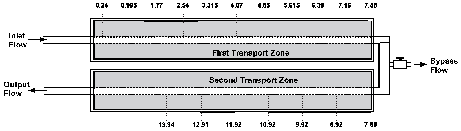
Figure 2. Algorithm for solving the system of equations.

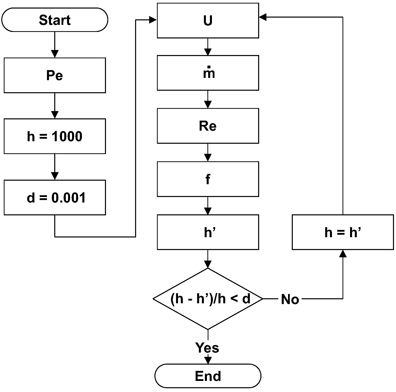
Figure 3. Control volumes and conservation of energy.

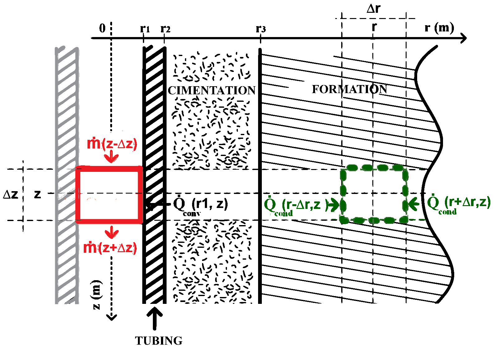
Figure 4. Transient functions.

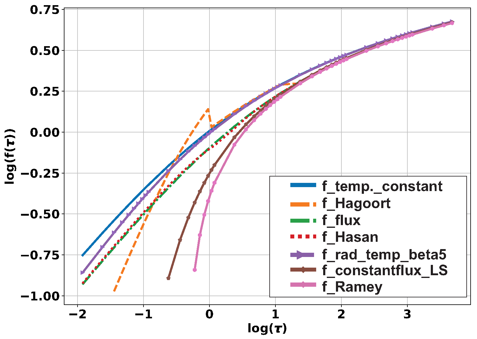
Figure 5. Transient functions - Dependence on problem conditions.

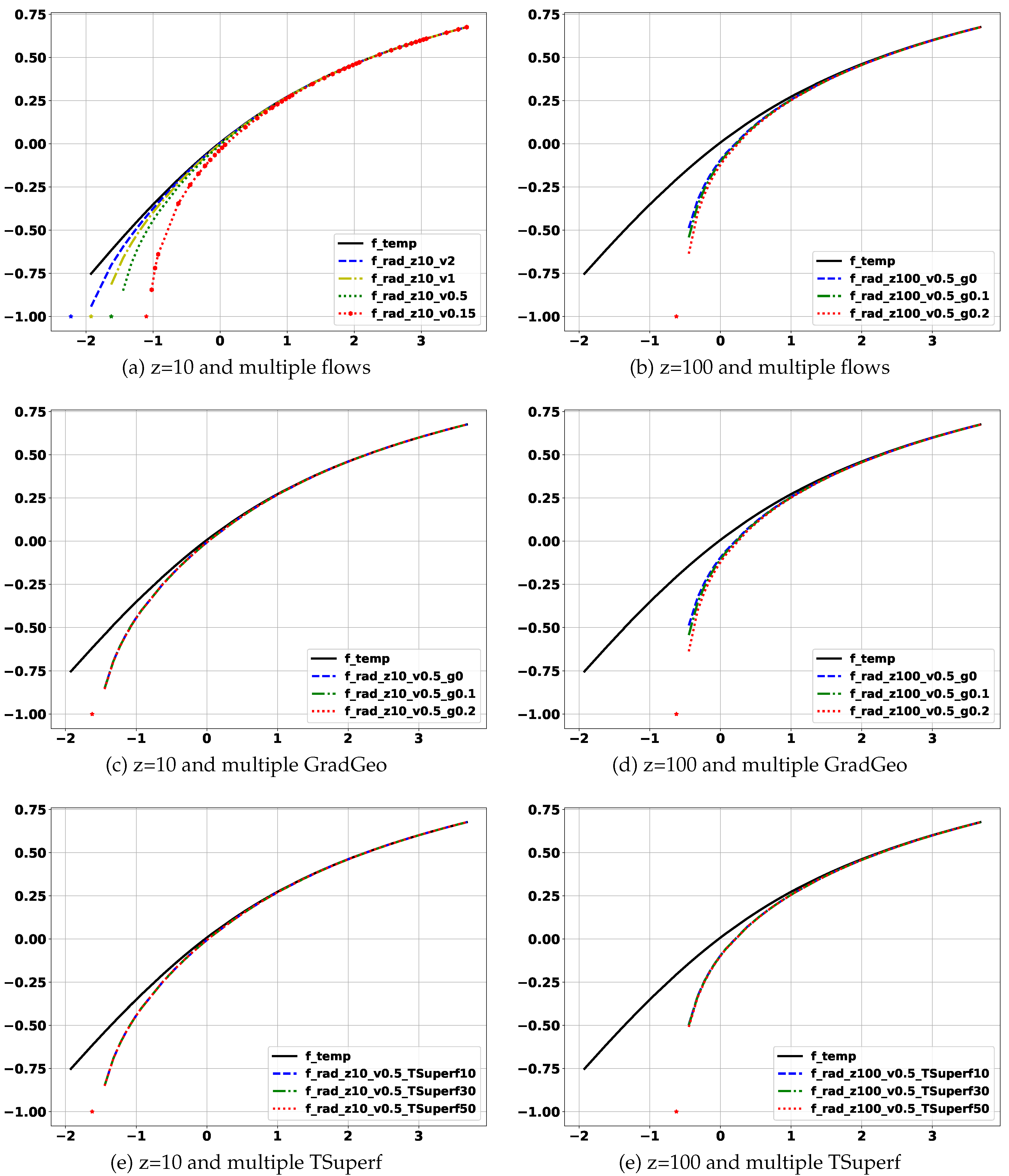
Figure 6. Real evolution of temperature with depth.

Figure 7. Simplified completion.

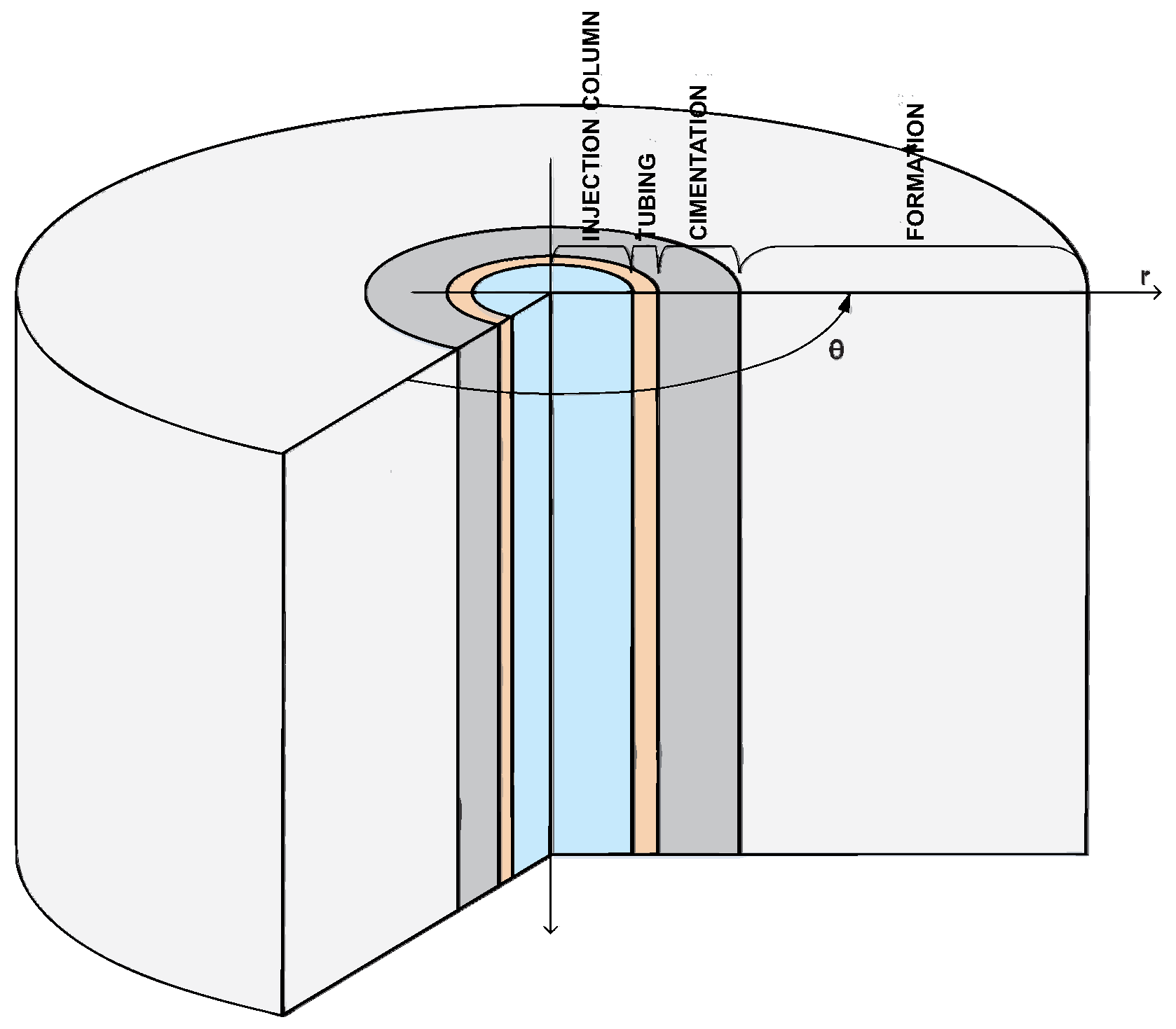
Figure 8. Boundary conditions.

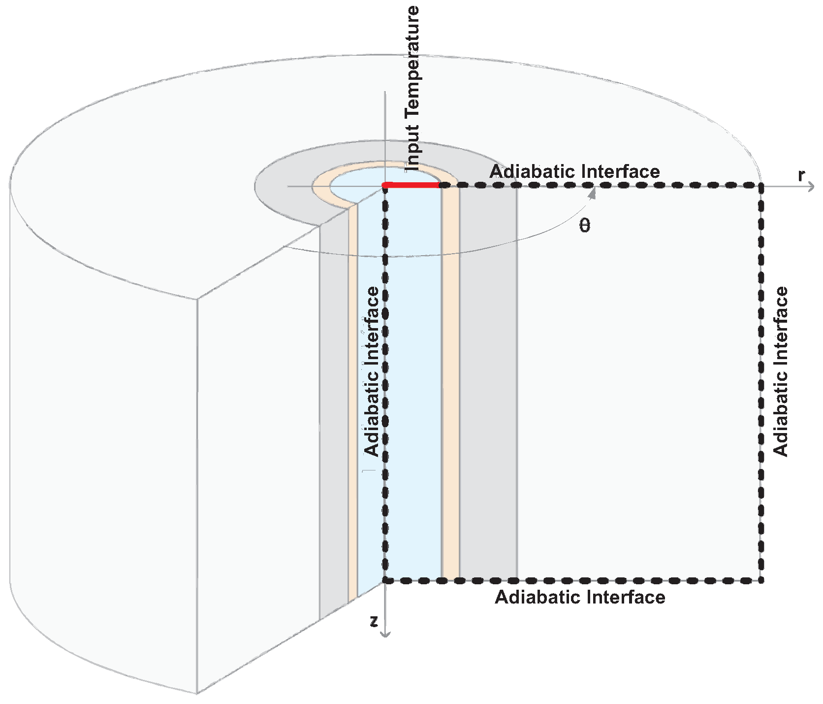
Figure 9. Subdivision of the domain and definition of measurement points.

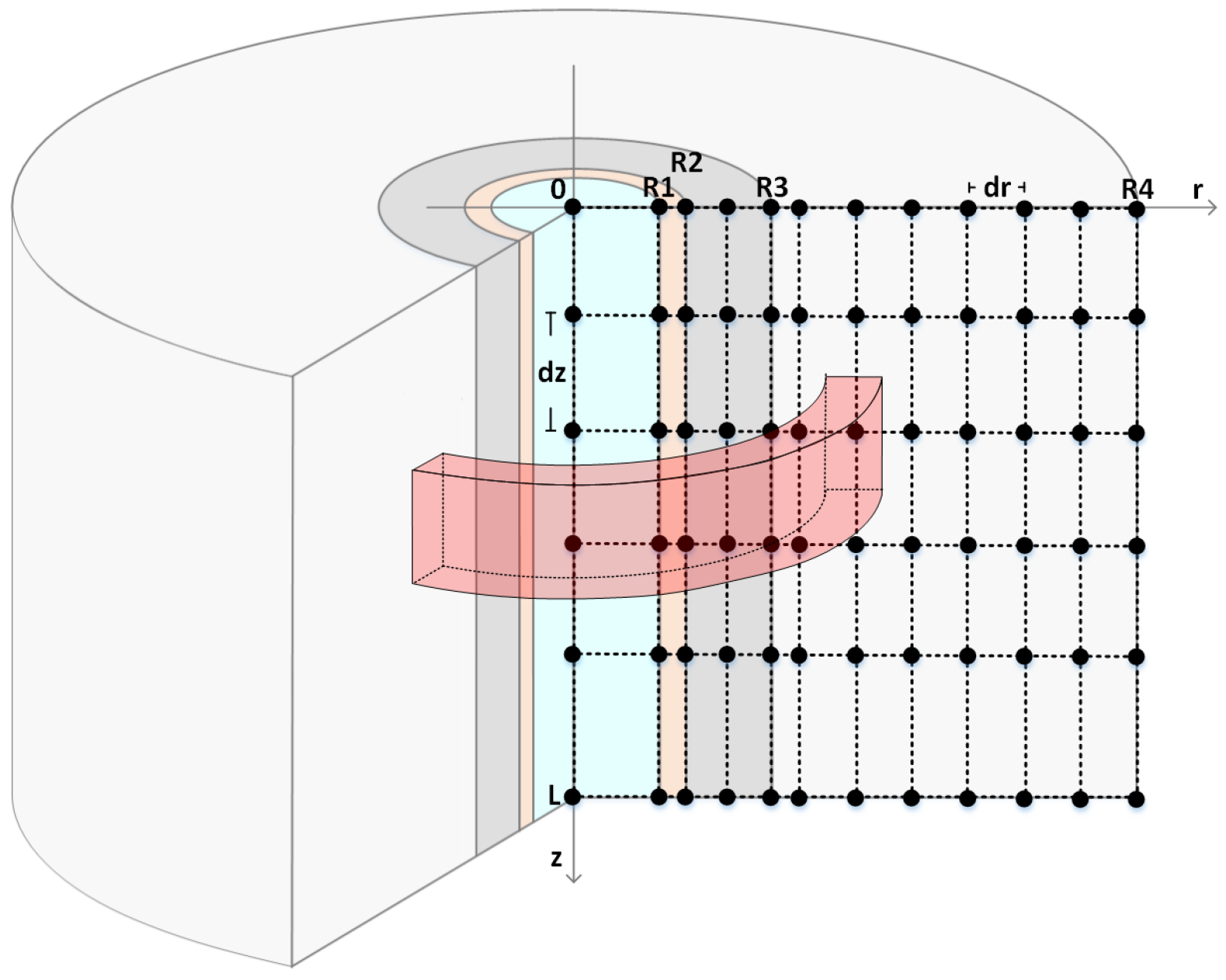
Figure 10. Discretization of temperature.

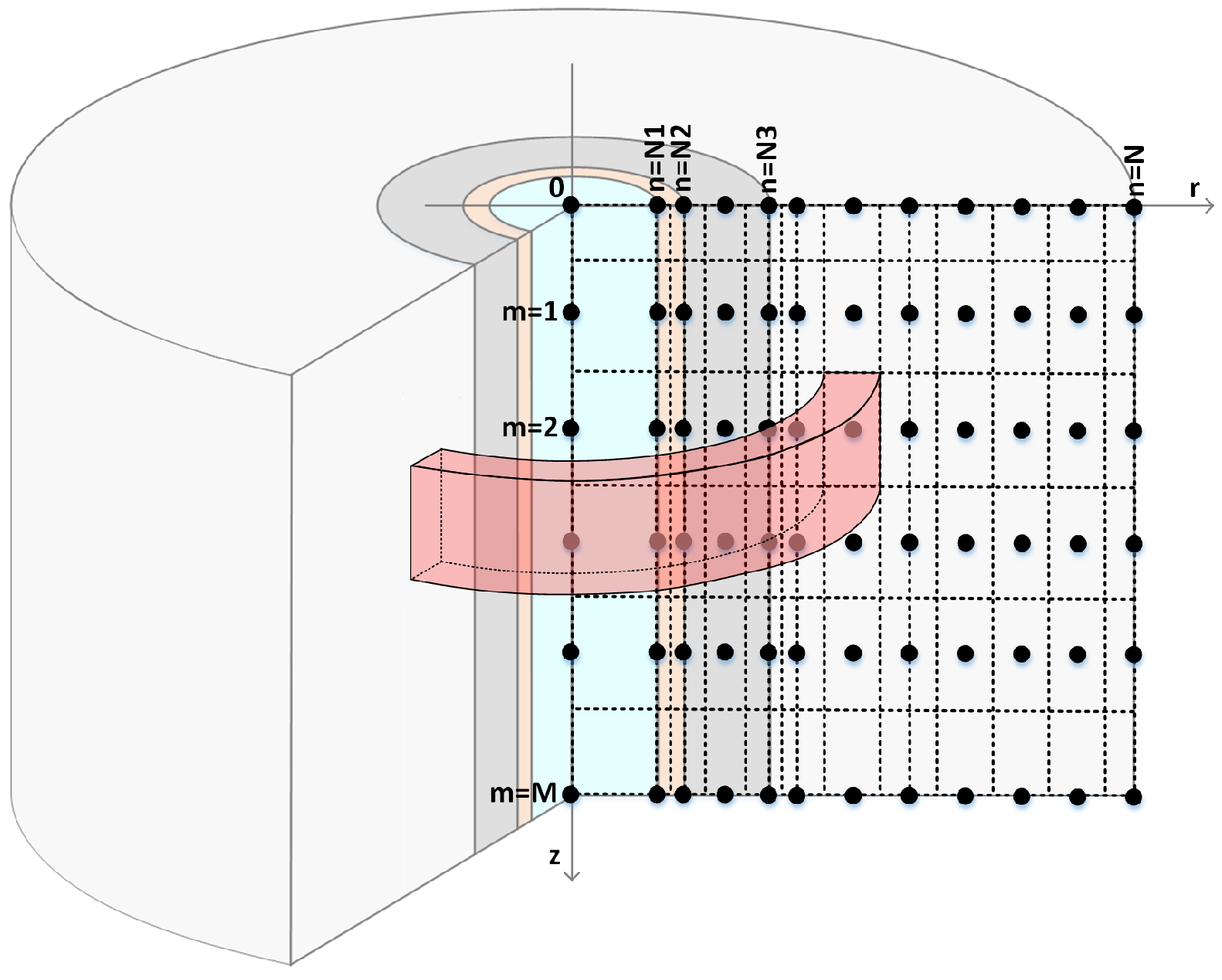
Figure 11. Discretization of properties.

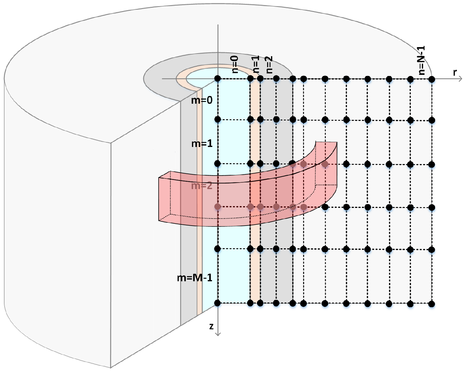
Figure 12. Areas, volumes, and their codes.

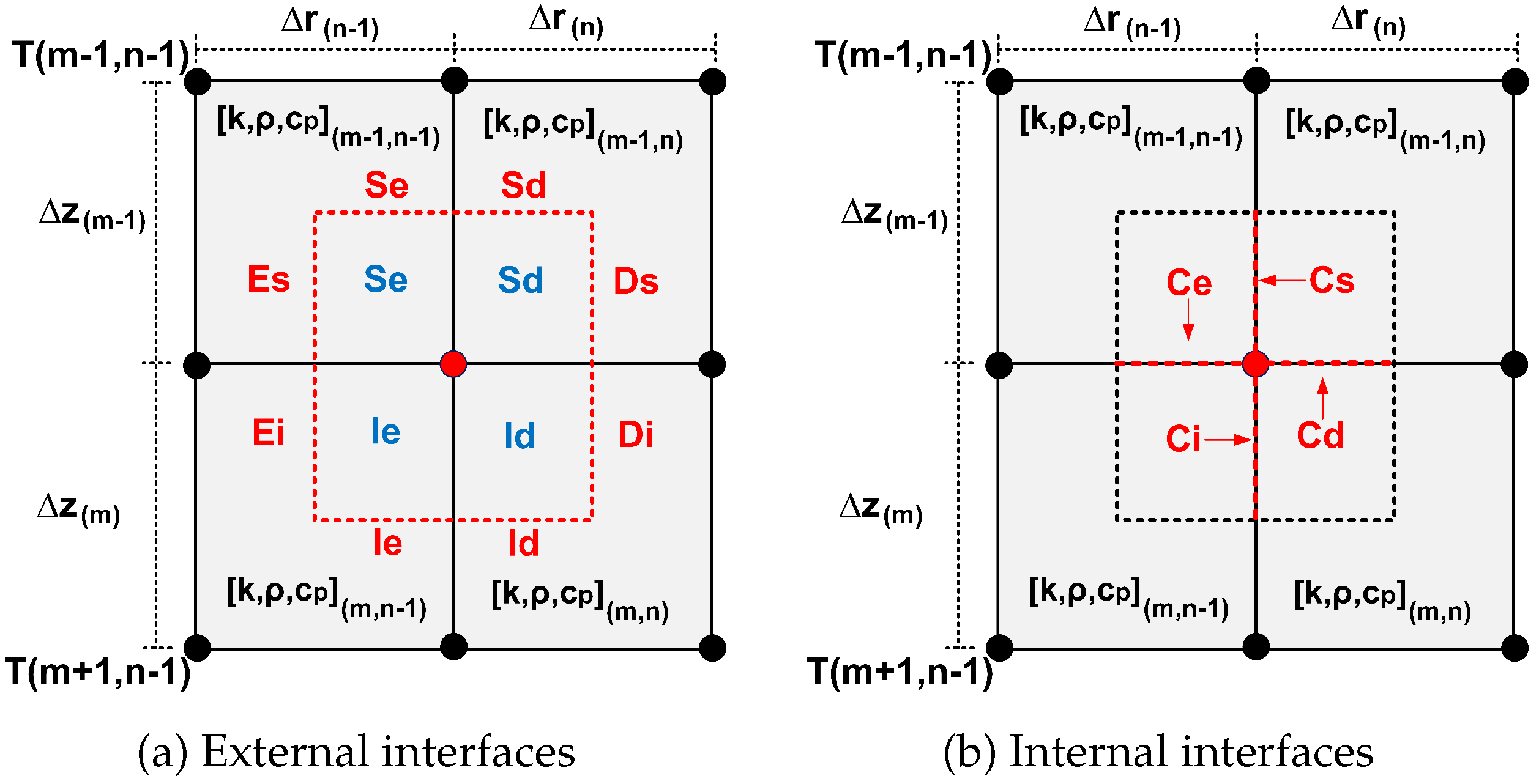
Figure 13. Control volumes with convection/conduction type interfaces.

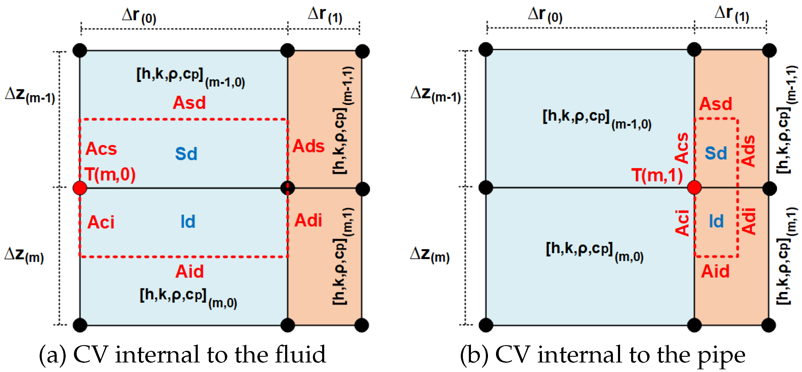
Figure 14. Conduction/conduction type interface - approach 1.

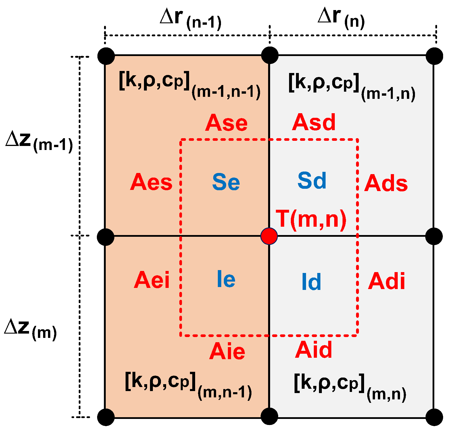
Figure 15. Conduction/conduction type interface - approach 2.

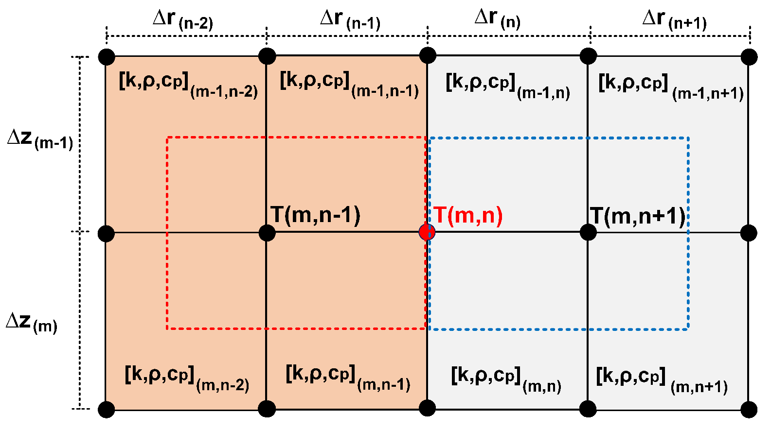
Figure 16. Well not completed - Detailing the problem.

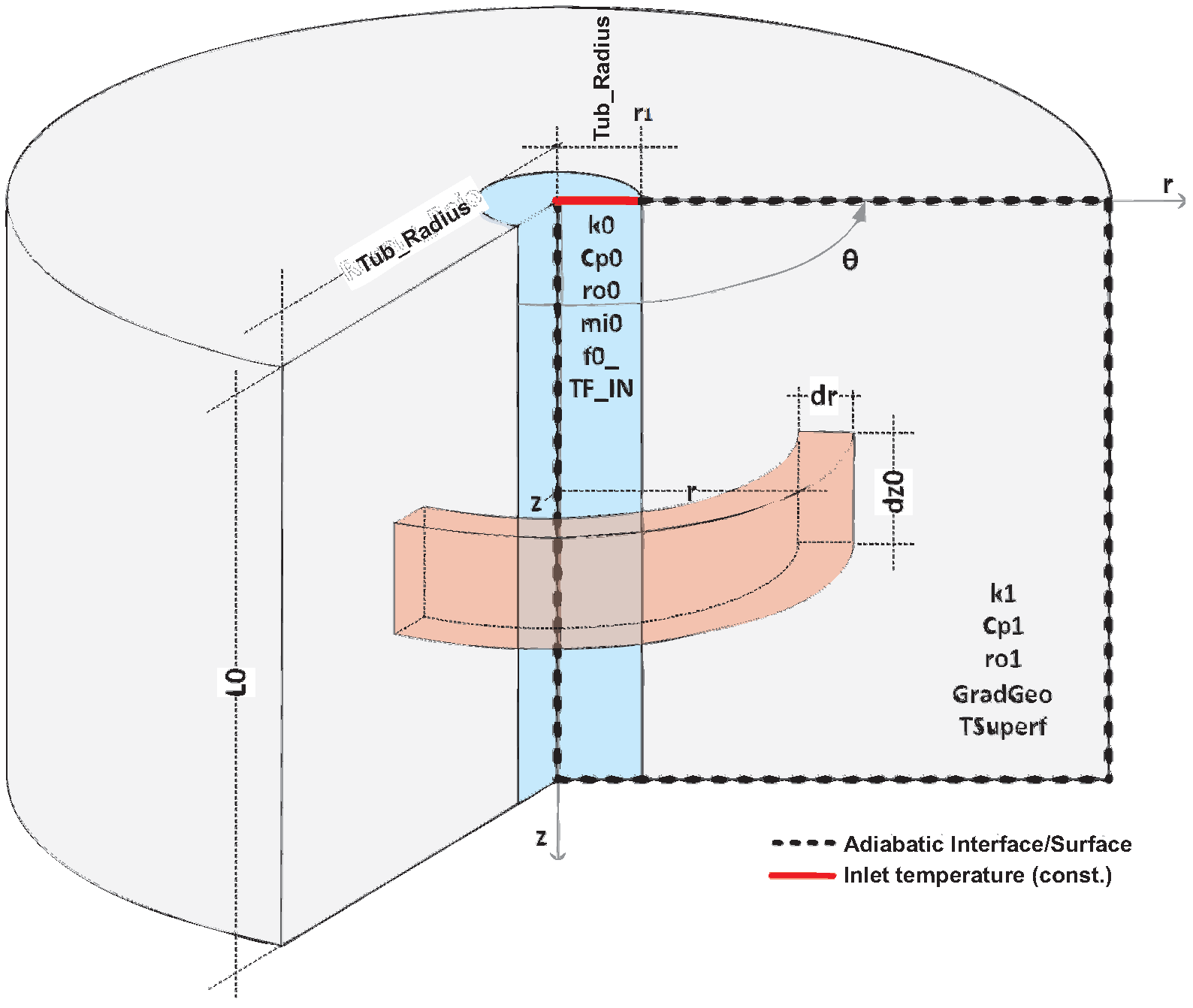
Figure 17. Uncompleted well - Longitudinal temperature evolution.

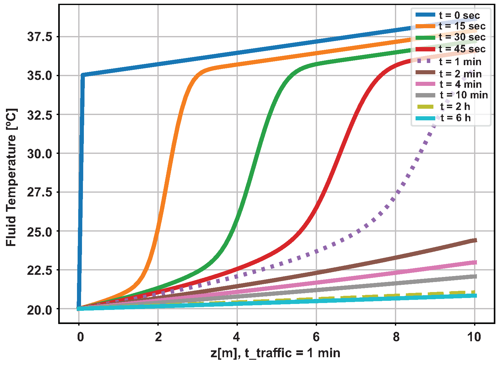
Figure 18. Uncompleted well - Radial temperature evolution.

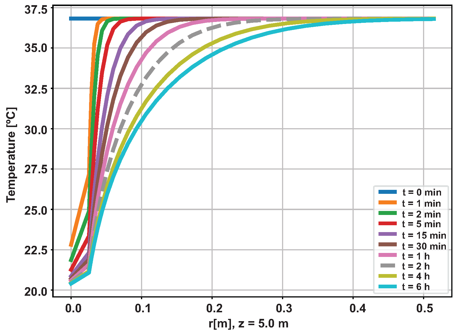
Figure 19. Uncompleted well - Measurement at 9 meters.

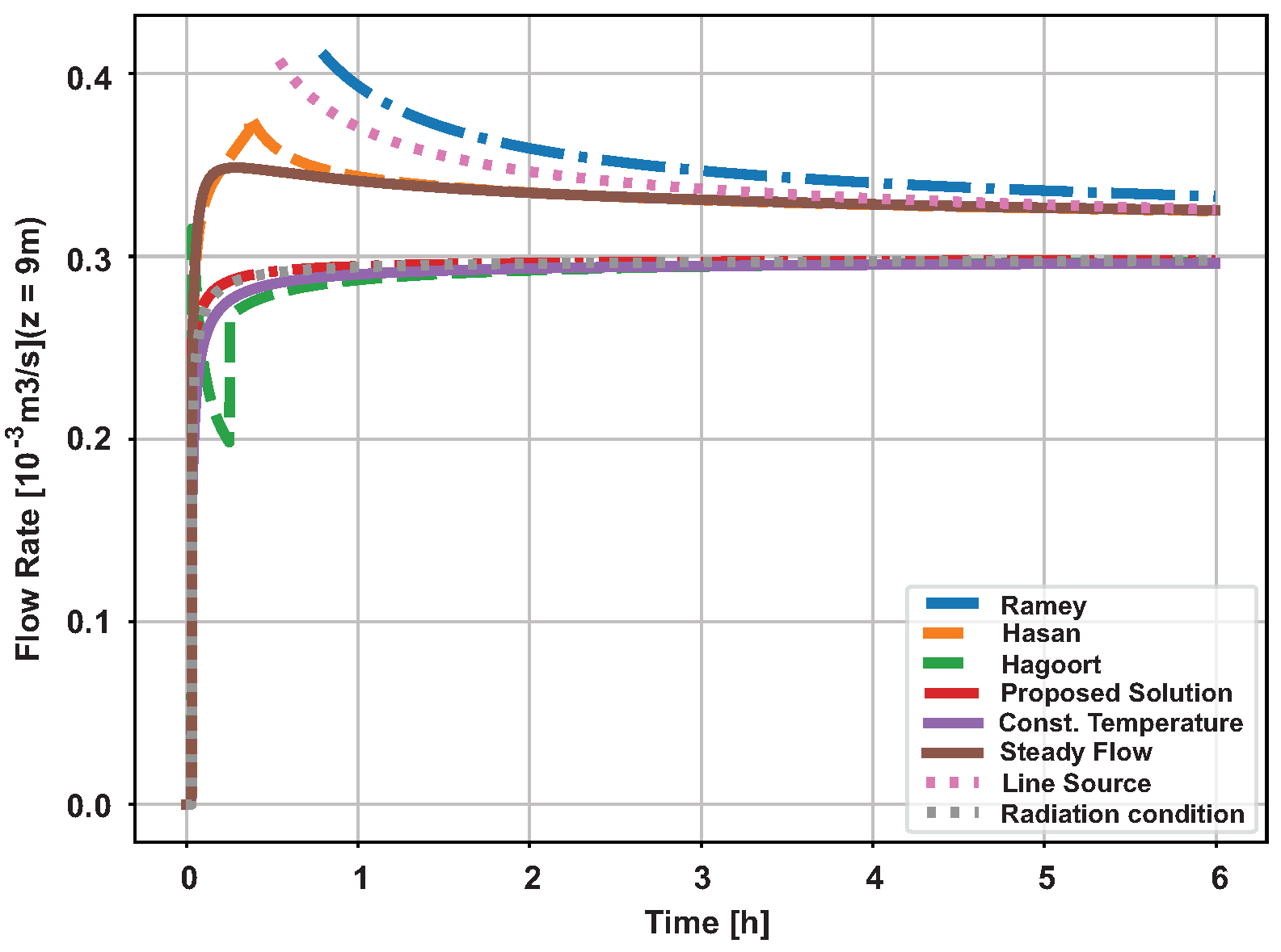
Figure 20. Uncompleted well - Evolution of measurement error.

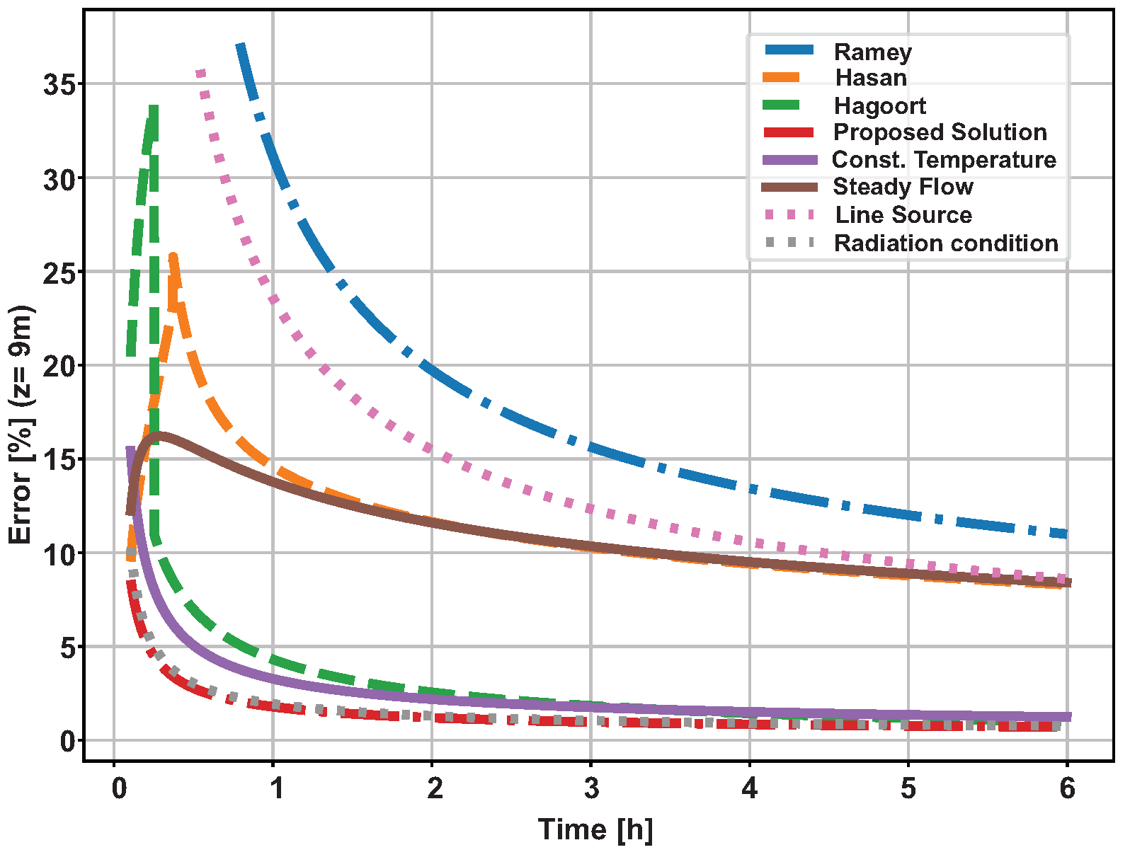
Figure 21. Two layer completion - Problem detail.

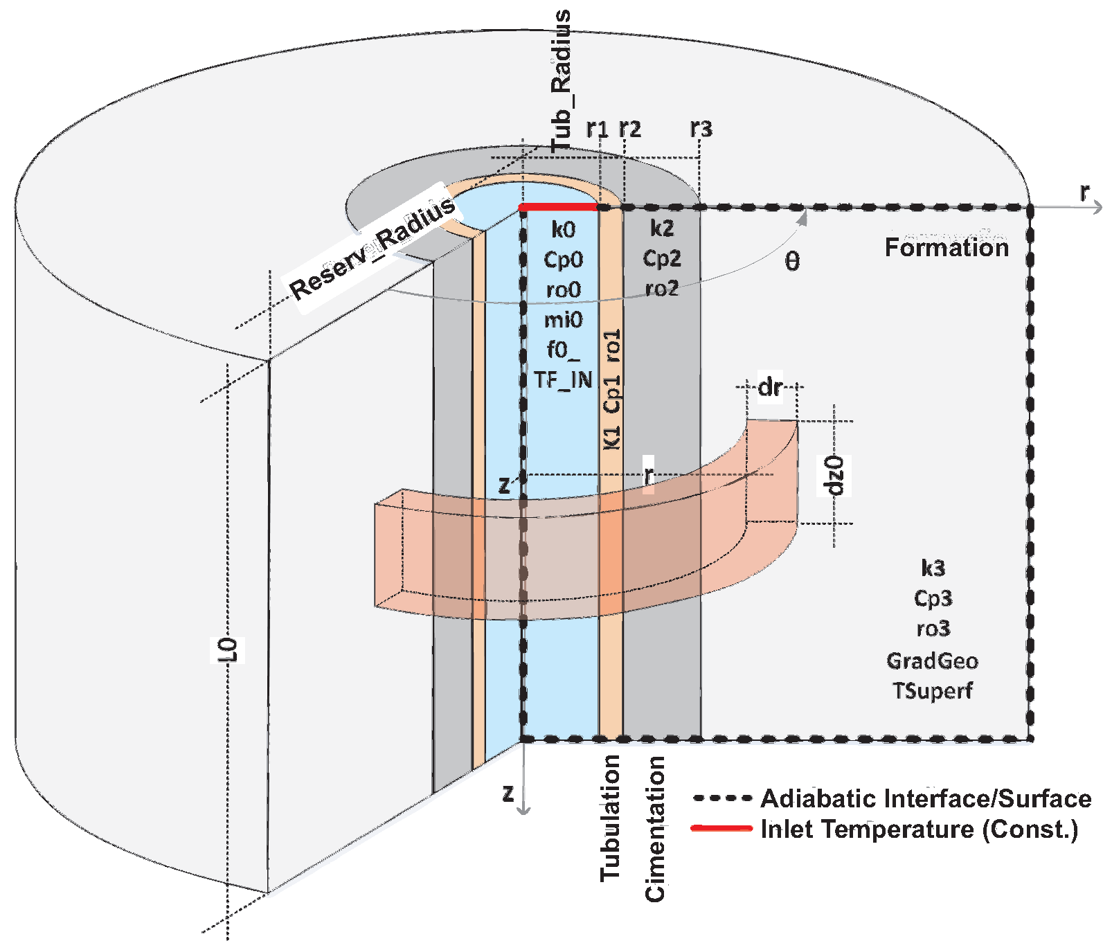
Figure 22. Completion with two layers - Longitudinal temperature evolution.

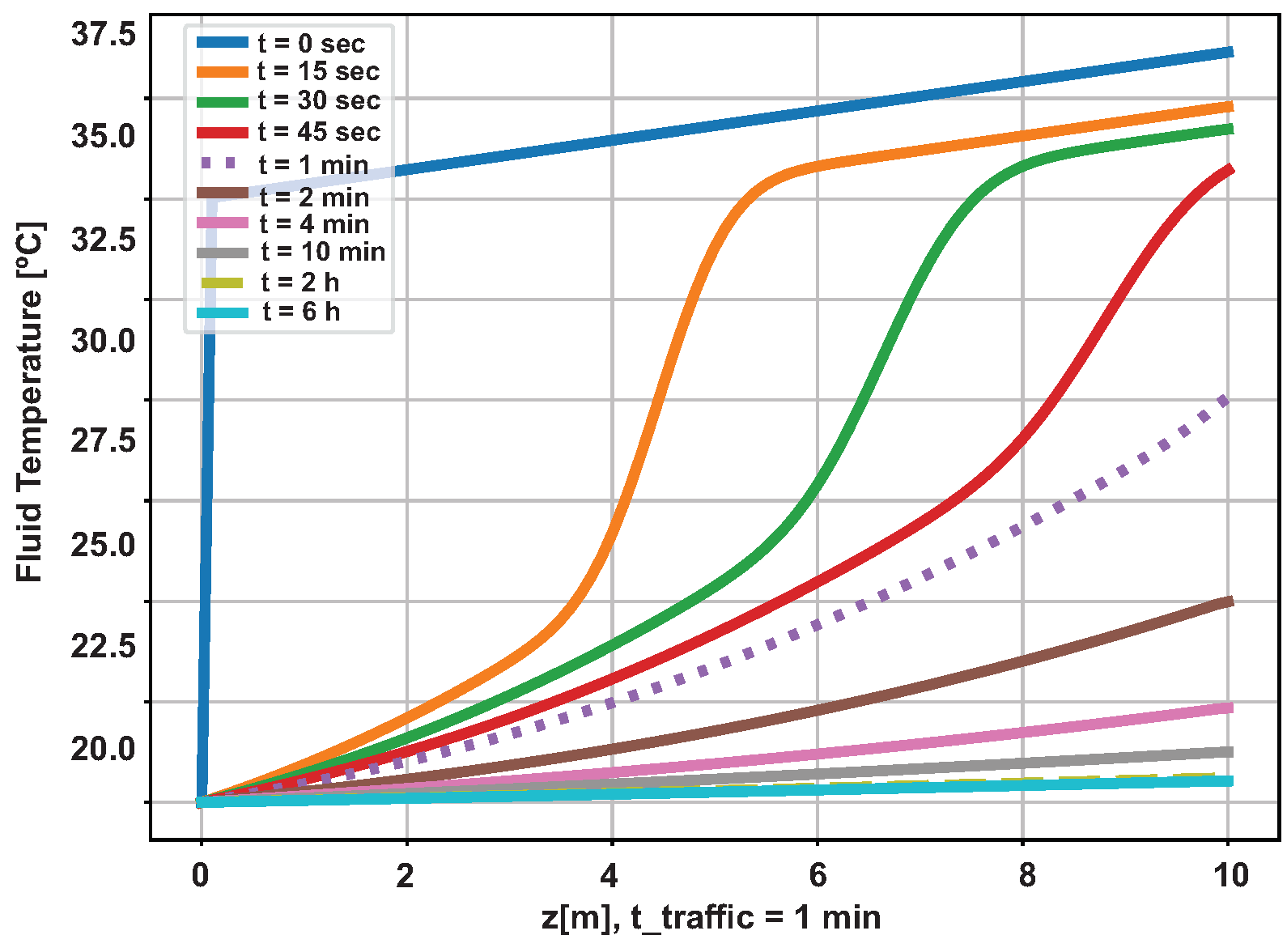
Figure 23. Completion with two layers - Radial temperature evolution (z=5m).

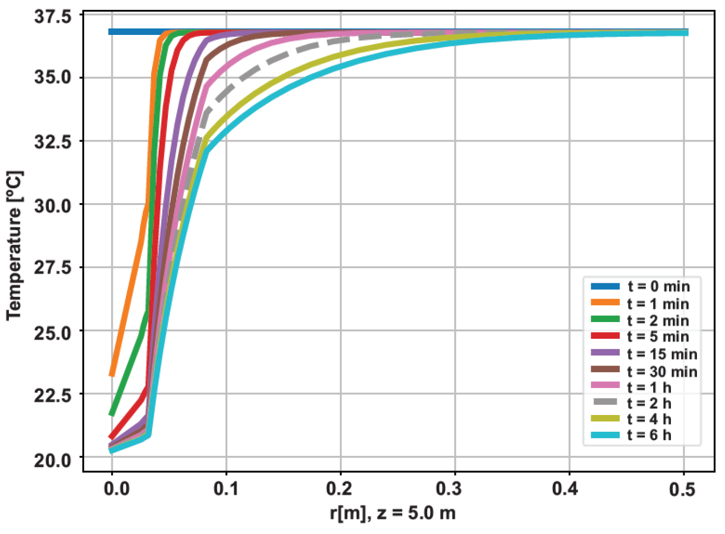
Figure 24. Uncompleted well - Longitudinal temperature evolution.

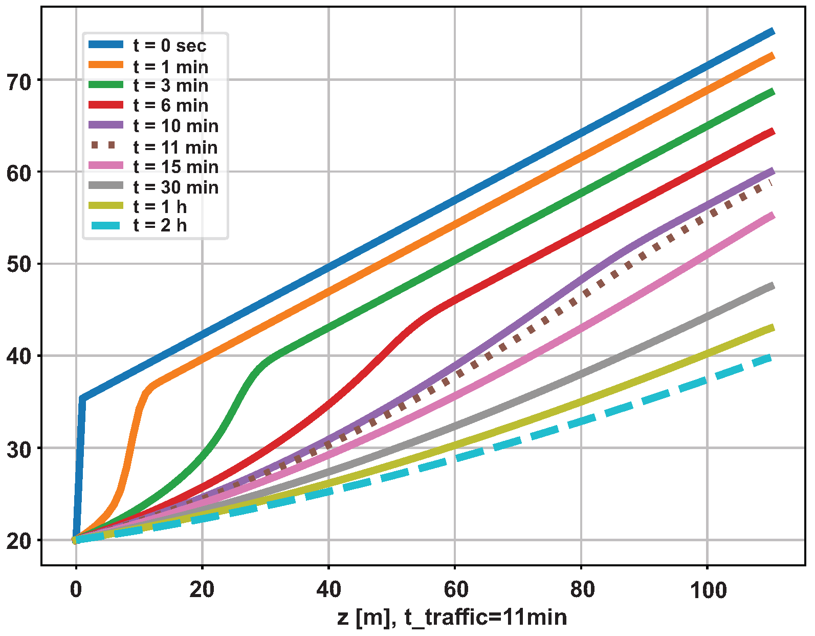
Figure 25. Uncompleted well - Measurement at 100 meters.

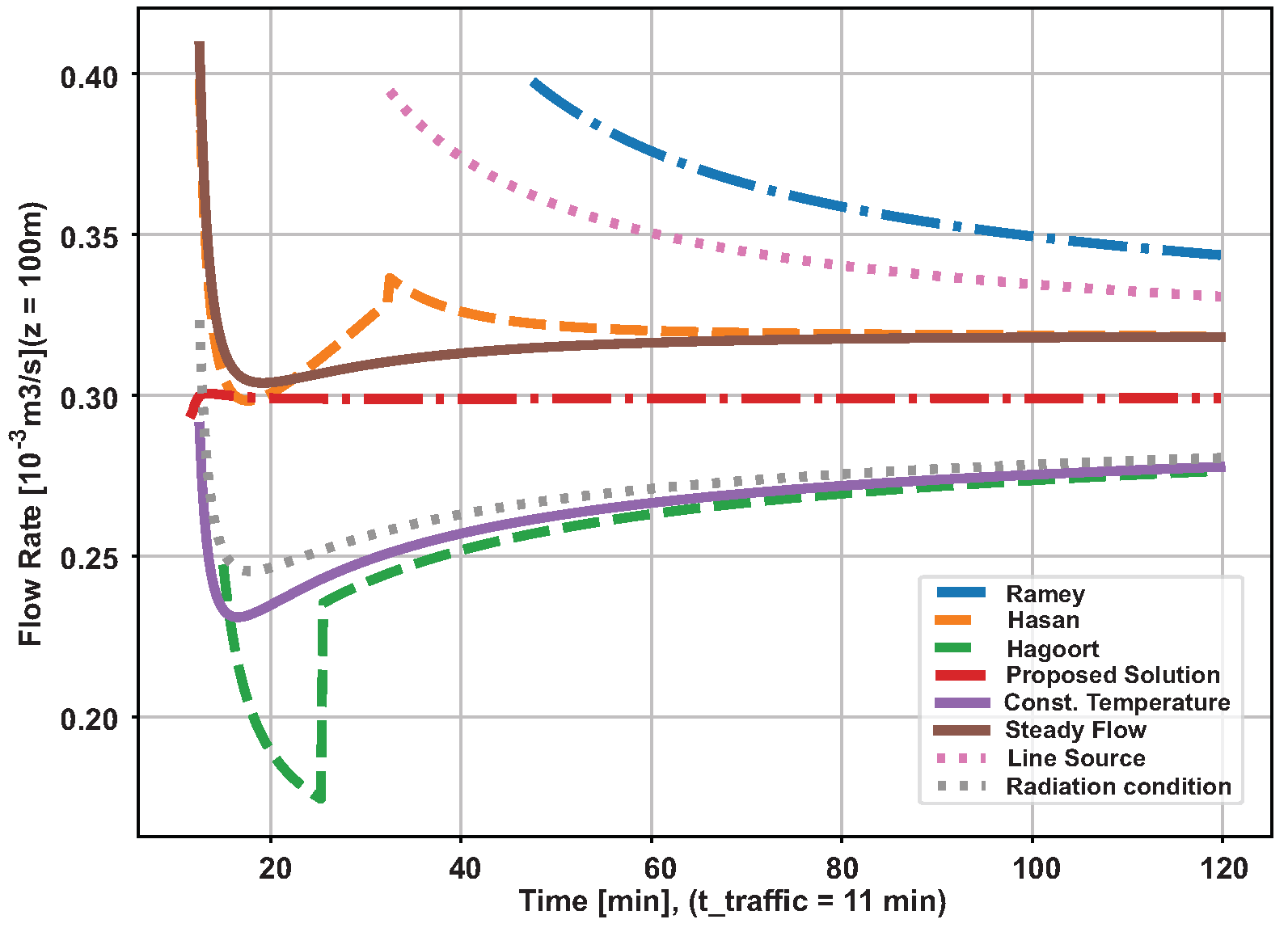
Figure 26. Error propagation in flow calculation - General data.

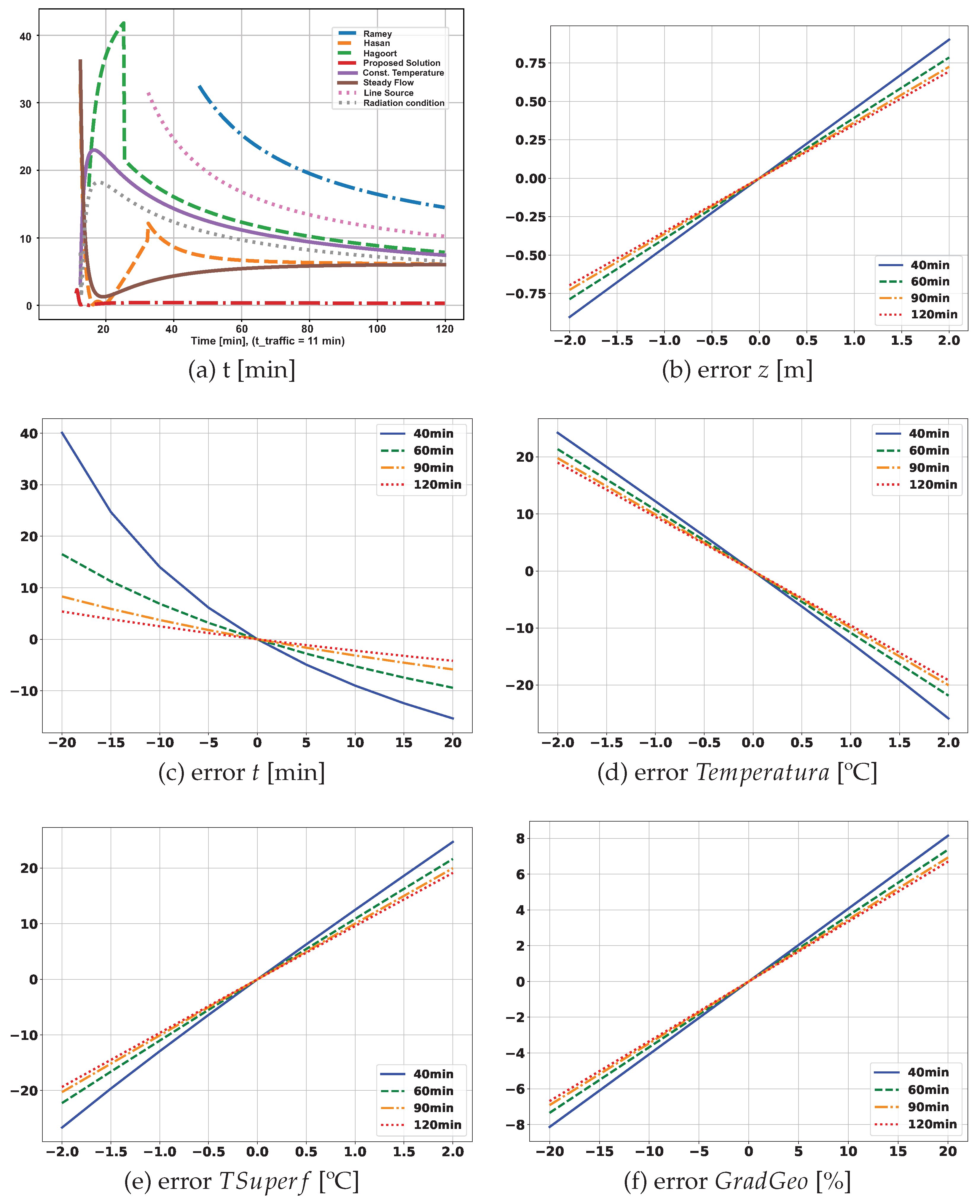
Figure 27. Error propagation in flow calculation - Physical properties.

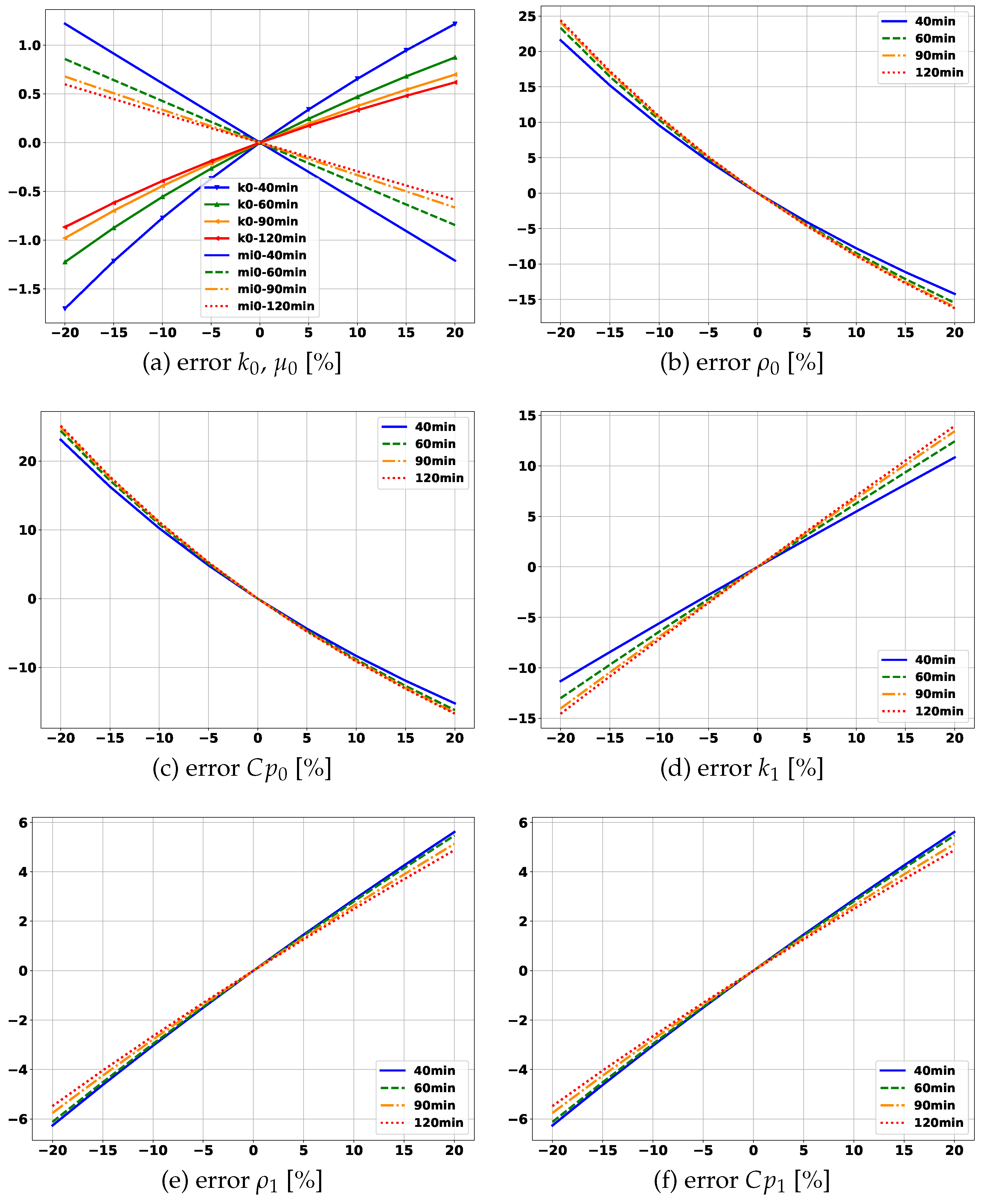
Table 1. System of differential equations - Simplified completion.

	Description	Equation
Formation ( $r_{3} \leq r \leq \infty$ )
	General Equation	$\frac{\partial^{2} T (r, z, t)}{\partial r^{2}} + \frac{1}{r} \frac{\partial T (r, z, t)}{\partial r} = \frac{1}{α_{3}} \frac{\partial T (r, z, t)}{\partial t}$ , $α_{3} = \frac{k_{3}}{ρ_{3} c_{3}}$
	Initial Condition	$T (r, z, 0) = T_{g} (z)$
	Boundary Condition (∞)	$\underset{r \to \infty}{l i m} T (r, z, t) = T_{g} (z)$
	Boundary Condition ( $r_{3}$ )	a) $k_{2} \frac{\partial T (r_{3}^{-}, z, t)}{\partial r} = k_{3} \frac{\partial T (r_{3}^{+}, z, t)}{\partial r}$
		b) $T (r_{3}^{-}, z, t) = T (r_{3}^{+}, z, t)$
Cimentation ( $r_{2} \leq r \leq r_{3}$ )
	General Equation	$\frac{\partial^{2} T (r, z, t)}{\partial r^{2}} + \frac{1}{r} \frac{\partial T (r, z, t)}{\partial r} = \frac{1}{α_{2}} \frac{\partial T (r, z, t)}{\partial t}$ , $α_{2} = \frac{k_{2}}{ρ_{2} c_{2}}$
	Initial Condition	$T (r, z, 0) = T_{g} (z)$
	Boundary Condition ( $r_{3}$ )	a) $k_{2} \frac{\partial T (r_{3}^{-}, z, t)}{\partial r} = k_{3} \frac{\partial T (r_{3}^{+}, z, t)}{\partial r}$
		b) $T (r_{3}^{-}, z, t) = T (r_{3}^{+}, z, t)$
	Boundary Condition ( $r_{2}$ )	a) $k_{1} \frac{\partial T (r_{2}^{-}, z, t)}{\partial r} = k_{2} \frac{\partial T (r_{2}^{+}, z, t)}{\partial r}$
		b) $T (r_{2}^{-}, z, t) = T (r_{2}^{+}, z, t)$
Tubing ( $r_{1} \leq r \leq r_{2}$ )
	General Equation	$\frac{\partial^{2} T (r, z, t)}{\partial r^{2}} + \frac{1}{r} \frac{\partial T (r, z, t)}{\partial r} = \frac{1}{α_{1}} \frac{\partial T (r, z, t)}{\partial t}$ , $α_{1} = \frac{k_{1}}{ρ_{1} c_{1}}$
	Initial Condition	$T (r, z, 0) = T_{g} (z)$
	Boundary Condition ( $r_{2}$ )	a) $k_{1} \frac{\partial T (r_{2}^{-}, z, t)}{\partial r} = k_{2} \frac{\partial T (r_{2}^{+}, z, t)}{\partial r}$
		b) $T (r_{2}^{-}, z, t) = T (r_{2}^{+}, z, t)$
	Boundary Condition ( $r_{1}$ )	a) $- r_{1}^{+} \frac{\partial T (r_{1}^{+}, z, t)}{\partial r} = β_{1} [T_{f} (z, t) - T (r_{1}^{-}, z, t)]$ , $β_{1} = \frac{r_{1} h}{k_{1}}$
		b) $T (r_{1}^{-}, z, t) = T (r_{1}^{+}, z, t)$
Fluid ( $0 \leq r \leq r_{1}$ )
	General Equation	$\frac{\partial T_{f} (z, t)}{\partial t} + v_{m e d} \frac{\partial T_{f} (z, t)}{\partial z} = \frac{2 h}{r_{1} ρ_{0} c_{0}} [T (r_{1}, z, t) - T_{f} (z, t)]$
	Initial Condition	$T_{f} (z, 0) = T_{g} (z)$
	Boundary Condition ( $z_{0}$ )	$T_{f} (0, t) = T_{f 0}$
	Boundary Condition ( $r_{1}$ )	a) $- r_{1}^{+} \frac{\partial T (r_{1}^{+}, z, t)}{\partial r} = β_{1} [T_{f} (z, t) - T (r_{1}^{-}, z, t)]$ , $β_{1} = \frac{r_{1} h}{k_{1}}$
		b) $T (r_{1}^{-}, z, t) = T (r_{1}^{+}, z, t)$

Table 2. Mapping

L o g_{10} (τ)

to dimensional time.

Table 2. Mapping

L o g_{10} (τ)

to dimensional time.

$L o g_{10} (τ)$	Dimensional time
-2	t=8.4 seconds
-1	t=84.0 seconds
0	t=14.0 minutes
1	t=2.3 hours
2	t=1.0 days
3	t=9.7 days

Table 3. Data used in the simulation without completion.

	Variable	Value	Description
Fluid	$k_{0}$	0.636 W/m.K	Thermal conductivity of water
	${C p}_{0}$	4.184 J/kg.K	Specific heat capacity of water
	$ρ_{0}$	1.000 kg/m³	Specific mass of water
	$μ_{0}$	0.0006 N.s/m²	Absolute viscosity
	${T f}_{0}$	80 ºC	Inlet fluid temperature
Formation	$k_{1}$	2.42 W/m.K	Thermal conductivity of the reservoir
	$C p_{1}$	1.500 J/kg.K	Specific thermal capacity of the reservoir
	$ρ_{1}$	2.100 kg/m³	Specific mass of the reservoir
	GradGeo	0.02 ºC/m	Geothermal gradient in dimension "z"
	TSuperf	10 ºC	Surface temperature

Table 4. Thermal fluxes - Equations.

Fluxs	Equation
${\dot{Q}}_{c o n d}$	$(k A_{n} / Δ z) [T (m + 1, n) - T (m, n)]$
${\dot{Q}}_{c o n d}$	$(k A_{n} / Δ z) [T (m - 1, n) - T (m, n)]$
${\dot{Q}}_{c o n d}$	$(k A_{n} / Δ r) [T (m, n + 1) - T (m, n)]$
${\dot{Q}}_{c o n d}$	$(k A_{n} / Δ r) [T (m, n - 1) - T (m, n)]$
${\dot{Q}}_{c o n v}$	$(h A_{n}) [T (m, n + 1) - T (m, n)]$
${\dot{Q}}_{c o n v}$	$(h A_{n} / Δ z) [T (m, n - 1) - T (m, n)]$
${\dot{M}}_{i n}$	$(\dot{m}) c_{j} T (m - 1, n)$
${\dot{M}}_{o u t}$	$- (\dot{m}) c_{j} T (m - 1, n)$

Table 5. Two layer completion - Data used in the simulation.

	Variable	Value	Description
General data	dt0	0.25 s	Time step
	dz0	0.1 m	Space step in the direction (longitudinal) z
	tsimu	6 h	Simulation time
	p_samples_z	0,1 m	Sampling period in the direction z
	p_samples_t	15 s	Time sampling period
	TAmb	35 °C	Room temperature
	TgeoType	1	Geothermal temperature type (0=constant; 1=linear)
	ThermalSource	0	0=Adiabatic Boundary; 1=Thermal source equal to Tgeo
Geometrics	L0	10 m	Longitudinal length of the well to be simulated
	Tub_Radius	0.0254 m	[r1] pipe inner radius
	Reserve_Radius	1 m	[r4] External radius of the reservoir
	DIV0	1	Number of radial divisions of the region 0
	DIV1	3	Number of radial divisions of the region 1
	DIV2	10	Number of radial divisions of the region 2
	DIV3	30	Number of radial divisions of the region 3
Fluid	$k_{0}$	0.636 $W / (m . K)$	Thermal conductivity of water
	$C p_{0}$	4.184 $J / (k g . K)$	Specific heat capacity of water
	$r o_{0}$	1.000 $k g / m^{3}$	Specific mass of water
	$m i_{0}$	0.0006 $N . s / m^{2}$	Absolute viscosity
	f0_	0.0003 $m^{3} / s$	Volume flow
	TF_IN	20 °C	Inlet fluid temperature
Tub	$k_{1}$	14 $W / (m . K)$	Thermal conductivity of the reservoir
	$C p_{1}$	502 $J / (k g . K)$	Specific thermal capacity of the reservoir
	$r o_{1}$	8.000 $k g / m^{3}$	Specific mass of the reservoir
	Tub_Thickness	0.635 $c m$	pipe thickness
Ciment	k2	0.9 $W / (m . K)$	Thermal conductivity of the reservoir
	Cp2	900 $J / (k g . K)$	Specific thermal capacity of the reservoir
	ro2	2.400 $k g / m^{3}$	Specific mass of the reservoir
	Cim_Thickness	5.08 $c m$	Cimentation thickness
Formation	k3	2.42 $W / (m . K)$	Thermal conductivity of the reservoir
	Cp3	1.500 $J / (k g . K)$	Specific thermal capacity of the reservoir
	ro3	2.100 $k g / m^{3}$	Specific mass of the reservoir
	GradGeo	0.365 °C/m	Geothermal gradient in the dimension z
	TSuperf	TAmb	Surface temperature

Table 6. Approximate rate of error propagation - 2 hours of operation.

	Variable	Error propagation rate
Measurement method	Ramey	15%
	Hasan	7%
	Hagoort	8%
	Temperature Constant	8%
	Temperature Constant e radiation	7%
	Flow Constant	7%
	Line Source	10%
	Analitic	0%
General	t [min]	-0.2 % / min
	z [m]	0.35 % / m
	T [ºC]	-9.5 % / ºC
	TSuperf [ºC]	9.5 % / ºC
Fluid	$k_{0}$ [%]	0.03
	$r o_{0}$ [%]	-1.2 / -0.8
	$C p_{0}$ [%]	-1.3 / -0.85
	$m i_{0}$ [%]	-0.04 / -0.03
Formation	$k_{1}$ [%]	0.7
	$r o_{1}$ [%]	0.235 / 0.22
	$C p_{1}$ [%]	0.235 / 0.22
	GradGeo [%]	0.31

Disclaimer/Publisher’s Note: The statements, opinions and data contained in all publications are solely those of the individual author(s) and contributor(s) and not of MDPI and/or the editor(s). MDPI and/or the editor(s) disclaim responsibility for any injury to people or property resulting from any ideas, methods, instructions or products referred to in the content.

© 2023 by the authors. Licensee MDPI, Basel, Switzerland. This article is an open access article distributed under the terms and conditions of the Creative Commons Attribution (CC BY) license (http://creativecommons.org/licenses/by/4.0/).

Copyright: This open access article is published under a Creative Commons CC BY 4.0 license, which permit the free download, distribution, and reuse, provided that the author and preprint are cited in any reuse.

Submitted:

28 March 2023

Posted:

29 March 2023

You are already at the latest version

Alerts

Abstract

Keywords:

Subject: Physical Sciences - Fluids and Plasmas Physics

1. Introduction

Two-inch (

0.0508

> 15 %

2. Mathematical Model and General Conditions

> 5 %

> 15 %

2.1. Solution with Double Thermal Profile

The flow measurement problem in injection wells of water and no phase change is governed by the equation:

\begin{matrix} \dot{m} = \frac{2 π r_{1} U (R, z, t)}{c (z, t)} [T (R, z, t) - T_{f} (z, t)] / \frac{\partial T_{f} (z, t)}{\partial z} - π {(r_{1})}^{2} ρ (z, t) \frac{\partial T_{f} (z, t)}{\partial t} / \frac{\partial T_{f} (z, t)}{\partial z} \end{matrix}

(1)

\begin{matrix} \frac{\partial T_{f} (z, t)}{\partial z} ≅ \frac{2 π r_{1} U (R, z, t)}{c (z, t) \dot{m} (z, t)} [T (R, z, t) - T_{f} (z, t)] - \frac{π {(r_{1})}^{2} ρ (z, t)}{\dot{m} (z, t)} \frac{\partial T_{f} (z, t)}{\partial t} \end{matrix}

(2)

\begin{matrix} \frac{\partial T_{f} (z, t)}{\partial z} & ≅ & \frac{2 π r_{1} U (R, z, t)}{c \dot{m}} [T (R, z, t) - T_{f} (z, t)] - \frac{π {(r_{1})}^{2} ρ (z, t)}{\dot{m}} \frac{\partial T_{f} (z, t)}{\partial t} \end{matrix}

(3)

Integrating Equation (3) from

z_{1}

z_{2}

, we have

\begin{matrix} \dot{m} & ≅ & \frac{2 π r_{1}}{c} \frac{\int_{z_{1}}^{z_{2}} U (R, z, t) (T (R, z, t) - T_{f} (z, t)) d z}{T_{f} (z_{2}, t) - T_{f} (z_{1}, t)} - π {(r_{1})}^{2} ρ (z, t) \frac{\int_{z_{1}}^{z_{2}} [\partial T_{f} (z, t) / \partial t] d z}{T_{f} (z_{2}, t) - T_{f} (z_{1}, t)} \end{matrix}

(4)

Assuming

\bar{U} (R, z, t)

to be the average value of

U (R, z, t)

in the interval

[z_{1}, z_{2}]

, it is worth approximation

\begin{matrix} \dot{m} & ≅ & \frac{2 π r_{1} \bar{U} (R, z, t)}{c} \frac{\int_{z_{1}}^{z_{2}} (T (R, z, t) - T_{f} (z, t)) d z}{T_{f} (z_{2}, t) - T_{f} (z_{1}, t)} - π {(r_{1})}^{2} ρ (z, t) \frac{\int_{z_{1}}^{z_{2}} [\partial T_{f} (z, t) / \partial t] d z}{T_{f} (z_{2}, t) - T_{f} (z_{1}, t)} \end{matrix}

(5)

where the value of

\bar{U} (R, z, t)

is given by

\begin{matrix} \frac{1}{\bar{U} (r, t)} & ≅ & [\frac{1}{h (r_{1})} + r_{1} (\frac{f_{t u b} (t)}{k_{t u b}} + \frac{f_{c o m b} (t)}{r_{2} h_{c o m b}} + \frac{f_{r e v} (t)}{k_{r e v}} + \frac{f_{c i m} (t)}{k_{c i m}}) + \frac{f (t)}{k_{f o r}}] \end{matrix}

(6)

The functions

f_{t u b} (t), f_{c o m b (t)}, f_{r e v (t)}, f_{c i m (t)}

and

f (t)

For t big enough, that is, for a

t > > t^{'}

, where

t^{'}

is such that

R = r_{5} e^{f (t^{'})}

, all significant transience for the calculation of the overall heat transfer coefficient is restricted to the transience of heat propagation in the formation beyond the radial position R, we have

\begin{matrix} \frac{1}{\bar{U} (R)} & ≅ & [\frac{1}{h (\dot{m})} + r_{1} (\frac{l n (\frac{r_{2}}{r_{1}})}{k_{t u b}} + \frac{1}{r_{2} h_{c o m b}} + \frac{l n (\frac{r_{4}}{r_{3}})}{k_{r e v}} + \frac{l n (\frac{r_{5}}{r_{4}})}{k_{c i m}} + \frac{l n (\frac{R}{r_{5}})}{k_{f o r}})] \end{matrix}

(7)

\bar{U}

, which, in turn, depends on the convection coefficient in the inner surface of the pipe,

h (\dot{m})

, which is a non-linear function of the intended flow estimate. In these terms, the resolution of the aforementioned equations for

\dot{m}

˙ depends on the knowledge of an additional independent relation between h and

\dot{m}

˙. For this, the Gnielinski equation will be used, resulting in a system of nonlinear equations. The flow calculation,

\dot{m}

˙, depends on the resolution of the composite nonlinear system by the following equations:

\begin{matrix} P_{r} & = & \frac{μ c}{k_{f}} \end{matrix}

(8)

\begin{matrix} R e & = & \frac{ρ v_{m e d} (2 r_{1})}{μ} \end{matrix}

(9)

\begin{matrix} f & = & {[0.79 l n (R e) - 1.64]}^{- 2} \end{matrix}

(10)

\begin{matrix} h & = & \frac{(f / 8) (R e - 1000) P_{r}}{1 + 12.7 {(f / 8)}^{0.5} ({P_{r}}^{2 / 3} - 1)} \frac{k_{f}}{2 r_{1}} \end{matrix}

(11)

\begin{matrix} \frac{1}{\bar{U}} & ≅ & {[\frac{1}{h} + \frac{r_{1}}{k_{t u b}} l n (\frac{r_{2}}{r_{1}}) + \frac{r_{1}}{r_{2} h_{c o m b}} + \frac{r_{1}}{k_{r e v}} l n (\frac{r_{4}}{r_{3}}) + \frac{r_{1}}{k_{c i m}} l n (\frac{r_{5}}{r_{4}}) + \frac{r_{1}}{k_{f o r}} l n (\frac{R}{r_{5}})]}^{- 1} \end{matrix}

(12)

\begin{matrix} \dot{m} & ≅ & \frac{2 π r_{1} \bar{U}}{c} \frac{\int_{z_{1}}^{z_{2}} (T (R, z, t) - T_{f} (z, t)) d z}{T_{f} (z_{2}, t) - T_{f} (z_{1}, t)} - π {(r_{1})}^{2} ρ \frac{\int_{z_{1}}^{z_{2}} [\partial T_{f} (z, t) / \partial t] d z}{T_{f} (z_{2}, t) - T_{f} (z_{1}, t)} \end{matrix}

(13)

where

P_{r}

is the Prandtl number,

R e

is the Reynolds number, f is the friction factor, h is the coefficient of convection given by the Gnielinski equation,

\bar{U}

is the overall heat transfer coefficient average in the interval

[z_{1}, z_{2}]

and

\dot{m}

˙ is the mass flow.

2.2. Quasi-Static Solution (Ramey Method)

T (R, z, t)

will correspond to the geothermal temperature,

T_{g} (z)

\dot{m}

, can be calculated by

\begin{matrix} \dot{m} & ≅ & \frac{2 π R_{1} \bar{U}}{c} \frac{\int_{z_{1}}^{z_{2}} (T_{g} (z) - T_{f}) d z}{T_{f} (z_{2}) - T_{f} (z_{1})} \end{matrix}

(14)

In this way, the remaining significant time dependence for the flow calculation lies in the formation-related transient function,

f (t)

\begin{matrix} P_{r} & = & \frac{μ c}{k_{f}} \end{matrix}

(15)

\begin{matrix} R e & = & \frac{ρ v_{m e d} (2 r_{1})}{μ} \end{matrix}

(16)

\begin{matrix} f & = & {[0.79 l n (R e) - 1.64]}^{- 2} \end{matrix}

(17)

\begin{matrix} h & = & \frac{(f / 8) (R e - 1000) P_{r}}{1 + 12.7 {(f / 8)}^{0.5} ({P_{r}}^{2 / 3} - 1)} \frac{k_{f}}{2 r_{1}} \end{matrix}

(18)

\begin{matrix} \frac{1}{\bar{U}} & ≅ & {[\frac{1}{h} + \frac{r_{1}}{k_{t u b}} l n (\frac{r_{2}}{r_{1}}) + \frac{r_{1}}{r_{2} h_{c o m b}} + \frac{r_{1}}{k_{r e v}} l n (\frac{r_{4}}{r_{3}}) + \frac{r_{1}}{k_{c i m}} l n (\frac{r_{5}}{r_{4}}) + \frac{r_{1}}{k_{f o r}} l n (\frac{R}{r_{5}})]}^{- 1} \end{matrix}

(19)

\begin{matrix} \dot{m} & ≅ & \frac{2 π R_{1} \bar{U}}{c} \frac{\int_{z_{1}}^{z_{2}} (T_{g} (z) - T_{f}) d z}{T_{f} (z_{2}) - T_{f} (z_{1})} \end{matrix}

(20)

2.3. Analytical Solution to Proposed Method

\begin{matrix} θ_{f} (z, t) & = & \frac{T_{f} (z, t) - T_{g} (z)}{T_{g} (z)} \end{matrix}

(21)

\begin{matrix} θ_{1} (z, t) & = & \frac{T (r_{1}, z, t) - T_{g} (z)}{T_{g} (z)} \end{matrix}

(22)

Since the convective heat flux at the inner interface of the pipe must be equal to the heat flux at the same interface due to the use of the global heat coefficient, there is

\begin{matrix} U (z, t) & = & h \frac{T_{f} (z, t) - T (r_{1}, z, t)}{T_{f} (z, t) - T_{g} (z)} \end{matrix}

(23)

and consequently:

\begin{matrix} U (z, t) & = & h - \frac{θ_{1} (z, t)}{θ_{f} (z, t)} h \end{matrix}

(24)

In this context, thermal energy flows only in the radial direction

(r)

, from the well to the reservoir, when the fluid temperature inside the pipeline is higher than the reservoir temperature, and from the reservoir to the well, otherwise.

Consider the control volumes (

C V

) generated by the revolution of the represented rectangles in Figure 3 around the center of the pipe, at

r = 0

. The first

C V

, represented by a red rectangle in the left part of the figure, inside the injection column, corresponds to a cylinder of radius

r_{1}

and height

Δ z

. It presents convective heat flux

(Q_{h})

and mass

(\dot{m})

. The second

C V

, dotted green rectangle in the right part of the figure, inside of the formation, at position

(r, z)

, corresponds to a rectangular ring of internal radius

r - \frac{Δ r}{2}

, radius external

r + \frac{Δ r}{2}

and height

Δ z

. Shows only heat flow by conduction

(Q_{k})

in the direction radial, due to the neglect of heat flow in the vertical direction. The application of the principles of conservation of energy and mass in the

C V

The resulting system solution, whose resolution is detailed in Appendix A [10], will be given by

\begin{matrix} θ_{f} (w, τ) & = & \frac{1}{T_{g} (w)} [- a_{w} L_{s \to τ}^{- 1} (\frac{1 - e^{- g (s) w}}{s g (s)}) + b_{w} θ_{f 0} L_{s \to τ}^{- 1} (\frac{e^{g (s)}}{s})] \end{matrix}

(25)

\begin{matrix} T_{f} (w, τ) & = & T_{g} (w) [- a_{w} L_{s \to τ}^{- 1} (\frac{1 - e^{- g (s) w}}{s g (s)}) + (T_{f 0} - T_{g 0}) θ_{f 0} L_{s \to τ}^{- 1} (\frac{e^{g (s)}}{s})] \end{matrix}

(26)

where

τ

is the dimensionless time, w is the dimensionless vertical coordinate,

θ f 0

is the temperature dimensionless fluid at

w = 0

a_{w}

is the geothermal gradient related to the dimensionless coordinate w and

b_{w}

is the linear coefficient of the dimensionless geothermal temperature. The values of

τ

, w,

a_{w}

and

b_{w}

are respectively given by:

\begin{matrix} τ & = & \frac{k_{1}}{ρ_{1} c_{1} r_{1}^{2}} t \end{matrix}

(27)

\begin{matrix} w & = & \frac{k_{1}}{v_{m e d} ρ_{1} c_{1} r_{1}^{2}} z \end{matrix}

(28)

\begin{matrix} a_{w} & = & \frac{v_{m e d} ρ_{1} c_{1} r_{1}^{2}}{k_{1}} a_{z} \end{matrix}

(29)

\begin{matrix} b_{w} & = & T_{g} (0) \end{matrix}

(30)

The function

g (s)

in equation (25) aims to simplify the notation. It is given by

\begin{matrix} g (s) & = & 2 α_{1} β_{1} [1 - θ_{1}^{'} (s)] + s \end{matrix}

(31)

where the function

θ_{1}^{'} (s)

does not depend on the radial coordinate. It is related to the temperature dimensionless

θ_{1} (w, τ)

, in

r_{1}

, by

\begin{matrix} θ_{1} (w, τ) = L_{s \to τ}^{- 1} (θ_{1}^{'} (s) θ_{f} (w, s)) \end{matrix}

(32)

As a consequence:

θ_{1} (w, τ) = \frac{1}{T_{g} (w)} [- a_{w} L_{s \to τ}^{- 1} (θ_{1}^{'} (s) \frac{1 - e^{- g (s) w}}{s g (s)}) + b_{w} θ_{f 0} (w, s) L_{s \to τ}^{- 1} (θ_{1}^{'} (s) \frac{e^{- g (s) w}}{s g (s)})]

(33)

where

\begin{matrix} θ_{1}^{'} (w, s) & = & c_{11}^{'} I_{0} (\sqrt{S}) - c_{12}^{'} K_{0} (\sqrt{S}) \end{matrix}

(34)

The functions

I_{0} (\sqrt{S})

and

K_{0} (\sqrt{S})

of equation (34) are known in the literature as functions modified Bessel models of the first and second types, respectively, both of zero order. To the variables

c_{11}^{'}

and

c_{12}^{'}

Thus, in addition to Equation (24), the overall heat coefficient can be rewritten as:

\begin{matrix} U (z, t) & = & h - \frac{- a_{w} L_{s \to τ}^{- 1} (θ_{1}^{'} (w, s) \frac{1 - e^{- g (s) w}}{s g (s)}) + b_{w} θ_{f 0} (w, s) L_{s \to τ}^{- 1} (θ_{1}^{'} (w, s) \frac{e^{- g (s) w}}{s g (s)})}{- a_{w} L_{s \to τ}^{- 1} (\frac{1 - e^{- g (s) w}}{s g (s)}) + b_{w} θ_{f 0} (w, s) L_{s \to τ}^{- 1} (\frac{e^{- g (s) w}}{s g (s)})} \end{matrix}

(35)

(τ < w)

. In this sense, the solution in question is only recommended for times superiors.

2.4. Considerations about the Transient Function

Consider the uncompleted well shown in Figure 4. The transient function for the calculation of heat propagation in the formation was defined by Ramey as [6]:

\begin{matrix} f (t) & = & \frac{2 π k_{1} [T (r_{1}, z, t) - T_{g} (z)] Δ z}{Δ Q (r_{1}, z, t)} \end{matrix}

(36)

or, considering the dimensionless representations:

\begin{matrix} f (t) & = & - θ (1, w, τ) / \frac{\partial θ (1, w, τ)}{\partial x} \end{matrix}

(37)

where

Δ Q

is the heat flux in r1 and x is the dimensionless radius, given by

x = \frac{r}{r_{1}}

In these terms, transient functions for boundary conditions such as temperature constant in

r_{1}

and constant flux in

r_{1}

are given, respectively, by:

\begin{matrix} f (τ) & = & 1 / L_{s \to τ}^{- 1} (\frac{K_{1} (\sqrt{s})}{\sqrt{s} K_{0} (\sqrt{s})}) \end{matrix}

(38)

\begin{matrix} f (τ) & = & L_{s \to τ}^{- 1} (\frac{K_{0} (\sqrt{s})}{s \sqrt{s} K_{1} (\sqrt{s})}) \end{matrix}

(39)

The transient function for the fluid with constant temperature and boundary condition of radiation in

r_{1}

can be expressed by

\begin{matrix} f (τ) & = & L_{s \to τ}^{- 1} (\frac{1}{s} \frac{K_{0} (\sqrt{s})}{K_{0} (\sqrt{s}) + \frac{\sqrt{s}}{β_{1}} K_{1} (\sqrt{s})}) / L_{s \to τ}^{- 1} (\frac{1}{\sqrt{s}} \frac{K_{0} (\sqrt{s})}{K_{0} (\sqrt{s}) + \frac{\sqrt{s}}{β_{1}} K_{1} (\sqrt{s})}) \end{matrix}

(40)

The transient function for the analytical solution proposed in this paper, which considers the variation of fluid temperature and the application of the radiation condition on

r_{1}

, is given by

\begin{matrix} f (τ) & = & \frac{- a_{w} L_{s \to τ}^{- 1} (χ (S) \frac{1 - e^{- g (s) w}}{s g (s)}) + b_{w} θ_{f 0} (w, s) L_{s \to τ}^{- 1} (χ (S) \frac{1 - e^{- g (s) w}}{s})}{- a_{w} L_{s \to τ}^{- 1} (φ (S) \frac{1 - e^{- g (s) w}}{s g (s)}) + b_{w} θ_{f 0} (w, s) L_{s \to τ}^{- 1} (φ (S) \frac{1 - e^{- g (s) w}}{s})} \end{matrix}

(41)

with

\begin{matrix} χ (S) & = & \frac{K_{0} (\sqrt{s})}{K_{0} (\sqrt{s}) + \frac{\sqrt{s}}{β_{1}} K_{1} (\sqrt{s})} \end{matrix}

(42)

\begin{matrix} φ (S) & = & \frac{\sqrt{s} K_{1} (\sqrt{s})}{K_{0} (\sqrt{s}) + \frac{\sqrt{s}}{β_{1}} K_{1} (\sqrt{s})} \end{matrix}

(43)

f_t e m p ._c o n s t a n t

curve corresponds to the constant temperature in

r_{1}

. The

f_H a g o o r t

curve, to the Hagoort approximation [5]. The

f_f l u x

curve, to the transfer function for the boundary condition of constant heat flux in

r_{1}

. The

f_H a s a n

curve, to Hasan approximation [9]. The

f_r a d_t e m p_b e t a 5

curve, to the solution assuming constant temperature in the fluid injection and applying the radiation boundary condition on

r_{1}

, assuming

β_{1} = 5

. The curve

f_c o n s t a n t f l u x_L S

, to the line source approach to heat flux. Finally, the

f_R a m e y

k_{1} = 2.42

\frac{W}{m . K}

ρ_{1} = 2100

\frac{k g}{m^{3}}

c_{1} = 1500

\frac{J}{k g . K}

and

r_{1} = 0.0254

Taking the transient function for the constant temperature (

f_t e m p

) in

r_{1}

(*)

T S u p e r f

), graphs (e) and (f) of Figure 5, as with the gradient, its impact depends on depth, but its intensity has little influence on the evolution of the curve.

3. Computer Simulation

3.1. Description of the Problem to Be Simulated

(r)

, angular

(θ)

coordinates and vertical

(z)

(r, θ, z)

are used. In addition, already assuming the existence of radial symmetry, the angular coordinate,

θ

, is neglected.

3.2. Numerical Method to Encode

C V

Δ x

, the better the approximation.

\begin{matrix} \frac{d_{g} (x)}{d x} ≅ \frac{g (x + Δ x) - g (x)}{Δ x} \end{matrix}

(44)

Δ t

, must meet the stability criterion of the method. The implicit approach does not present such limitation [13].

3.3. Subdivision of the Problem into Control Volumes

r_{1}

, outside radius of the pipe,

r_{2}

, outside radius of the cement,

r_{3}

, and radius of the formation,

r_{4}

3.4. Discretization of Temperature and Other Properties

3.5. Coding of Areas, Volumes, and Properties

(m, n)

. In that figure, the codes

S_{e}

=upper left,

S_{d}

=upper right,

I_{e}

=lower left, and

I_{d}

=lower right are related areas or sub-volumes, according to self-description. The codes Left=Left top,

E_{i}

=bottom left,

D_{s}

=top right, Di=bottom right,

C_{s}

=top center,

C_{i}

=lower center,

C_{e}

=left center and

C_{d}

=right center correspond to related areas of the control volume. Thus, as an example of the use of the code, the heat flux in time

(t - Δ t)

, in the upper left interface area of the control volume at

(m, n)

, is represented by ˙

{\dot{Q}}_{S e}^{t - Δ t}

. In turn, the energy contained in the upper left region of the same control volume, at the same instant of time is expressed by

\begin{matrix} E {(m, n)}_{S e}^{t - Δ t} & = & {(V ρ c)}_{S e} T {(m, n)}^{t - Δ t} \end{matrix}

(45)

where V represents the volume of the subdivision under analysis.

3.6. Formulation of Mathematical Equation

\begin{matrix} Δ E & = & Δ t [\sum {\dot{Q}}_{S e}^{t - Δ t} + \sum {(\dot{m} c)}_{i} T_{i}^{t - Δ t} + {\dot{E}}_{g e r}^{t - Δ t}] \end{matrix}

(46)

\begin{matrix} Δ E & = & Δ t [\sum {\dot{Q}}_{S e}^{t} + \sum {(\dot{m} c)}_{i} T_{i}^{t} + {\dot{E}}_{g e r}^{t}] \end{matrix}

(47)

The equation (46) corresponds to the explicit method, as already discussed. Equation (47) says respect to the implicit method. In both equations,

Δ t

is the iteration time increment,

\dot{Q}

is the rate of thermal energy exchanged with the surroundings,

\dot{m} c T

is the rate of energy received or provided by the

C V

as a result of the mass flow. The variables ˙Eger and

Δ E

are, respectively, the internal rate of energy generation and the change in the control volume energy. The indices superscripts (t and

t - Δ t

t - Δ t

), as well as the inexistence of an energy-generating source inside the control volume (

{\dot{E}}_{g e r} = 0

The change in energy,

Δ E

, can be expressed by

\begin{matrix} Δ E & = & {(V ρ c)}_{j} (T^{t} - T^{t - Δ t}) \end{matrix}

(48)

\begin{matrix} {(V ρ c)}_{j} (T^{t} - T^{t - Δ t}) & = & Δ t [\sum {\dot{Q}}_{i}^{t - Δ t} + \sum {(\dot{m} c)}_{i} T_{i}^{t - Δ t}] \end{matrix}

(49)

\begin{matrix} {(V ρ c)}_{j} (T^{t} - T^{t - Δ t}) & = & Δ t [\sum {\dot{Q}}_{i}^{t} + \sum {(\dot{m} c)}_{i} T_{i}^{t}] \end{matrix}

(50)

Because it is simpler to code, the explicit method is represented by the equation (49). That equation can be rewritten as

\begin{matrix} T^{t} & = & T^{t - Δ t} + \frac{\sum {\dot{Q}}_{i}^{t - Δ t} + \sum {(\dot{m} c)}_{i} T_{i}^{t - Δ t}}{\sum {(V ρ c)}_{j}} Δ t \end{matrix}

(51)

which defines the temperature update rule that is adopted.

\begin{matrix} Δ t & \leq & \frac{\sum {(V ρ c)}_{i}}{\sum {({\dot{Q}}_{c o e f})}_{i} + \sum {({\dot{M}}_{c o e f})}_{i}} \end{matrix}

(52)

where

\sum {(V ρ c)}_{i}

corresponds to the total control volume capacitance , while

\sum {({\dot{Q}}_{c o e f})}_{i}

and

\sum {({\dot{M}}_{c o e f})}_{i}

are the sums of all temperature coefficients

T (m, n)

involved in the heat transfer and mass transfer calculations, respectively.

By examining equation (52), it is evident that the maximum time increment

(Δ t)

\begin{matrix} [\sum {({\dot{Q}}_{c o e f})}_{i} + \sum {({\dot{M}}_{c o e f})}_{i}] Δ t & \leq & \sum {(V ρ c)}_{i} \end{matrix}

(53)

3.7. Boundary Conditions

3.7.1. Definitions

Consider that the control volumes interfaces can be classified according to the boundary condition to which it is submitted, that is:

1) constant temperature, 2) adiabatic, 3) convection/conduction, 4) radiation/conduction, and 5) conduction/conduction.

The type interfaces constant temperature and adiabatic are self-explanatory. The other interfaces, type

A / B

, refer to interfaces on which two methods of data transfer occur simultaneously heat in its adjacent surroundings: method A on the A side and method B on the B side.

3.7.2. Constant Temperature

The distribution of the

C V s

\begin{matrix} T {(m, n)}^{t + Δ t} = T {(m, n)}^{t} = c o n s t a n t \end{matrix}

(54)

for all temperature measurement points,

(m, n)

, contained in said interfaces.

3.7.3. Adiabatic Boundary

Boundary conditions of the adiabatic boundary type are conditions in which there is no heat transfer across the considered

C V

interface. Its insertion in the code will be done by the neglect of heat flow (by convection, conduction, radiation, or mass flow) by said interface, that is:

\begin{matrix} \dot{Q} {(m, n)}_{i}^{t + Δ t} = \dot{Q} {(m, n)}_{i}^{t} = 0 \end{matrix}

(55)

for all

V C (m, n)

sub-interfaces contained in the boundary interface, represented in the equation (54) by the letter i.

3.7.4. Convection/Conduction

C V

D s

(top right) and

D i

(bottom right), from the

C V

internal to the fluid, and at the

C s

interfaces (center top) and

C i

(bottom center), from the internal

C V

to the pipe.

3.7.5. Conduction/Conduction

Conducting/conducting type interface relies on calculating the gradient on both sides from the interface. Consequently, as discussed in the previous subsection, it will always be an approximation.

Consider the approach presented in Figure 14. Although the

C V

internally encompasses boundary sub-interfaces, none of its sub-interfaces are. That is, the properties thermodynamics of the inner region of the

C V

, immediately adjacent to its sub-interfaces, are the same properties as the immediately adjacent region outside the

C V

Now consider the approach depicted in Figure 15. In this, the adjacent

C V s

(m, n - 1)

and

(m, n + 1)

are expanded in the direction of the

C V (m, n)

. From the boundary condition and disregarding the coordinate m for purposes of simplifying the nomenclature, we have:

\begin{matrix} k (n - 1) \frac{\partial T^{-} (n)}{\partial r} - k (n + 1) \frac{\partial T^{+} (n)}{\partial r} = 0 \end{matrix}

(56)

\begin{matrix} \frac{\partial T^{-} (n)}{\partial r} + \frac{\partial T^{+} (n)}{\partial r} = 2 \frac{\partial \bar{T} (n)}{\partial r} \end{matrix}

(57)

where

\begin{matrix} \frac{\partial T^{-} (r)}{\partial r} = lim_{Δ r \to 0} \frac{\partial T (r - Δ r)}{\partial r} \end{matrix}

(58)

\begin{matrix} \frac{\partial T^{+} (r)}{\partial r} = lim_{Δ r \to 0} \frac{\partial T (r + Δ r)}{\partial r} \end{matrix}

(59)

\begin{matrix} \frac{\partial \bar{T} (n)}{\partial r} ≅ \frac{1}{2} [\frac{T (n) - T (n - 1)}{Δ r (n - 1)} + \frac{T (n + 1) - T (n)}{Δ r (n)}] \end{matrix}

(60)

with

\frac{\partial \bar{T} (n)}{\partial r}

being the average temperature gradient in

(m, n)

From equations (56) and (57), we have:

\begin{matrix} \frac{\partial T^{-} (n)}{\partial r} = \frac{2 k (n)}{k (n - 1) + k (n)} \frac{\partial \bar{T} (n)}{\partial r} \end{matrix}

(61)

and consequently:

\begin{matrix} {\dot{Q}}^{-} (n) = {\dot{Q}}^{+} (n) ≅ - 2 A_{n} \frac{k (n - 1) k (n)}{k (n - 1) + k (n)} \frac{\partial \bar{T} (n)}{\partial r} \end{matrix}

(62)

which is the heat flux to be considered at the expanded boundary interface

C V s

4. Obtained Results

4.1. Simulation without Completion

4.1.1. Description

4.1.2. Simulation Data

The Table 5 brings the variables and values used in the simulation of this topic. The rest variables used in the simulation are functions of the presented values.

4.1.3. General Results

Figure 17 shows the temporal evolution of the fluid temperature along the pipeline.

1^{o} C

Figure 18 presents the temporal evolution of the radial temperature at a depth of

5.0

4.1.4. Inferred Flow

The graph in Figure 19 presents the flow measurement evolution for the methods and functions presented in [10]. As can be seen, all methods tend to converge to the reference flow

(0.3 \times 10^{- 3} [m^{3} / s])

. Still, methods derived from the assumption of constant temperature show better results

(Q_T e m p, Q_R A D_T C_{1} a n d Q_H a g o o r t)

The two best results

(Q_R A D_T C a n d Q_A n a l í t i c)

4.2. Simulation with Completion

4.2.1. Description

4.2.2. Simulation Data

Following the same way from the previous simulation, the other variables used are functions of the presented values.

4.2.3. General Results

5.0

5. Results with Error Propagation and Discussions

5.1. Simulation Data and Error Propagation

As shown in Table 5, on-page

21 a n d 22

, brings the variables and values used in this topic. Following the same approach as in the previous simulation, the other variables used are functions of the presented values.

1^{o} C

0.04

%, corresponding to an error propagation rate of

\frac{4}{500}

\frac{1}{1}

\frac{3}{4}

\frac{1}{4}

- 0.47 % (= - 2 * 0.235 %)

in the flow measurement. If the systematic error for the same variable is

+ 3

%, the systematic error in the flow measurement will be approximately

+ 0.66 % (= + 3 \times 0.22 %)

ρ_{0}

) and the thermal capacity (

C p_{0}

) of the fluid, as well as the thermal conductivity of the formation (

k_{1}

), do not decrease with the operation time, although, as can be seen in the graphs, it moves towards convergence at a limit value.

6. Conclusions

Author Contributions

Funding

This research was funded in part by Universidad Nacional de San Agustin de

Institutional Review Board Statement

Informed Consent Statement

Data Availability Statement

Conflicts of Interest

The authors declare no conflict of interest.

Abbreviations

The following abbreviations are used in this manuscript:

CV	Control Volume
DST	Distributed Sensors Temperature

References

Reges, J. E. O.; Salazar, A. O.; Maitelli, C. W. S. P.; Carvalho, L. G.; Britto, U. J. B. Flow Rates Measurement and Uncertainty Analysis in Multiple-Zone Water-Injection Wells from Fluid Temperature Profiles. Sensors 2016, 16(07), 1077. [Google Scholar] [CrossRef] [PubMed]
Shen, F.; Cheng, L.; Sun, Q.; Huang, S. Evaluation of the Vertical Producing Degree of Commingled Production via Waterflooding for Multilayer Offshore Heavy Oil Reservoirs. Energies 2018, 11(09), 2428. [Google Scholar] [CrossRef]
Silva, W. L. A.; Lima, V. S.; Fonseca, D. A. M.; Salazar, A. O.; Maitelli, C. W. S. P.; Echaiz, E. G. A. Study of Flow Rate Measurements Derived from Temperature Profiles of an Emulated Well by a Laboratory Prototype. Sensors 2019, 19(07), 1498. [Google Scholar] [CrossRef] [PubMed]
Ramírez, J.; Zambrano, A.; Ratkovich, N. Prediction of Temperature and Viscosity Profiles in Heavy-Oil Producer Wells Implementing a Downhole Induction Heater. Process 2023, 11(02), 631. [Google Scholar] [CrossRef]
Hagoort, J. Ramey’s wellbore heat transmission revisited. SPE journal, Society of Petroleum Engineers, 2004; 9, 465–474. [Google Scholar]
Ramey Jr, H.; Henry, J. Wellbore heat transmission. Journal of petroleum Technology 1962, 14(04), 427–435. [Google Scholar] [CrossRef]
Leutwyler, K. Casing temperature studies in steam injection wells. Journal of Petroleum Technology 1966, 18(09), 1157–1162. [Google Scholar] [CrossRef]
Wu, Y. S.; Pruess, K. An analytical solution for wellbore heat transmission in layered formations. SPE Reservoir Engineering 1990, 05(04), 531–538. [Google Scholar] [CrossRef]
Hasan, A. R.; Kabir, C. S. Aspects of wellbore heat transfer during two-phase flow. SPE Production & Facilities, 1994; 9, 211–216. [Google Scholar]
Lima, V. S. Perfis térmicos em poços injetores d’água: redução do erro sistemático na medição de vazão durante o regime transitório. Ph.D. Thesis, UFRN University, Natal, Brazil, 2019. (In Portuguese). [Google Scholar]
Jacquot, R.; Steadman, J.; Rhodine, C. The gaver-stehfest algorithm for approximate inversion of laplace transforms. IEEE Circuits & Systems Magazine, 1983; 5, 4–8. [Google Scholar]
Reges, J. E. O. Medição das vazões e análise de incerteza em poços Injetores de água Multizonas a Partir do Perfil de Temperatura do Fluido. Ph.D. Thesis, UFRN University, Natal, Brazil, 2016. (In Portuguese). [Google Scholar]
Çengel, Y. A.; Ghajar, A. J. Tranferência de calor e massa: uma abordagem prática. 4. ed. Porto Alegre: AMGH, xxii, 904 p., 2012. (In Portuguese)

Figure 1. Prototype installed at UFRN.

Figure 2. Algorithm for solving the system of equations.

Figure 3. Control volumes and conservation of energy.

Figure 4. Transient functions.

Figure 5. Transient functions - Dependence on problem conditions.

Figure 6. Real evolution of temperature with depth.

Figure 7. Simplified completion.

Figure 8. Boundary conditions.

Figure 9. Subdivision of the domain and definition of measurement points.

Figure 10. Discretization of temperature.

Figure 11. Discretization of properties.

Figure 12. Areas, volumes, and their codes.

Figure 13. Control volumes with convection/conduction type interfaces.

Figure 14. Conduction/conduction type interface - approach 1.

Figure 15. Conduction/conduction type interface - approach 2.

Figure 16. Well not completed - Detailing the problem.

Figure 17. Uncompleted well - Longitudinal temperature evolution.

Figure 18. Uncompleted well - Radial temperature evolution.

Figure 19. Uncompleted well - Measurement at 9 meters.

Figure 20. Uncompleted well - Evolution of measurement error.

Figure 21. Two layer completion - Problem detail.

Figure 22. Completion with two layers - Longitudinal temperature evolution.

Figure 23. Completion with two layers - Radial temperature evolution (z=5m).

Figure 24. Uncompleted well - Longitudinal temperature evolution.

Figure 25. Uncompleted well - Measurement at 100 meters.

Figure 26. Error propagation in flow calculation - General data.

Figure 27. Error propagation in flow calculation - Physical properties.

Table 1. System of differential equations - Simplified completion.

	Description	Equation
Formation ( $r_{3} \leq r \leq \infty$ )
	General Equation	$\frac{\partial^{2} T (r, z, t)}{\partial r^{2}} + \frac{1}{r} \frac{\partial T (r, z, t)}{\partial r} = \frac{1}{α_{3}} \frac{\partial T (r, z, t)}{\partial t}$ , $α_{3} = \frac{k_{3}}{ρ_{3} c_{3}}$
	Initial Condition	$T (r, z, 0) = T_{g} (z)$
	Boundary Condition (∞)	$\underset{r \to \infty}{l i m} T (r, z, t) = T_{g} (z)$
	Boundary Condition ( $r_{3}$ )	a) $k_{2} \frac{\partial T (r_{3}^{-}, z, t)}{\partial r} = k_{3} \frac{\partial T (r_{3}^{+}, z, t)}{\partial r}$
		b) $T (r_{3}^{-}, z, t) = T (r_{3}^{+}, z, t)$
Cimentation ( $r_{2} \leq r \leq r_{3}$ )
	General Equation	$\frac{\partial^{2} T (r, z, t)}{\partial r^{2}} + \frac{1}{r} \frac{\partial T (r, z, t)}{\partial r} = \frac{1}{α_{2}} \frac{\partial T (r, z, t)}{\partial t}$ , $α_{2} = \frac{k_{2}}{ρ_{2} c_{2}}$
	Initial Condition	$T (r, z, 0) = T_{g} (z)$
	Boundary Condition ( $r_{3}$ )	a) $k_{2} \frac{\partial T (r_{3}^{-}, z, t)}{\partial r} = k_{3} \frac{\partial T (r_{3}^{+}, z, t)}{\partial r}$
		b) $T (r_{3}^{-}, z, t) = T (r_{3}^{+}, z, t)$
	Boundary Condition ( $r_{2}$ )	a) $k_{1} \frac{\partial T (r_{2}^{-}, z, t)}{\partial r} = k_{2} \frac{\partial T (r_{2}^{+}, z, t)}{\partial r}$
		b) $T (r_{2}^{-}, z, t) = T (r_{2}^{+}, z, t)$
Tubing ( $r_{1} \leq r \leq r_{2}$ )
	General Equation	$\frac{\partial^{2} T (r, z, t)}{\partial r^{2}} + \frac{1}{r} \frac{\partial T (r, z, t)}{\partial r} = \frac{1}{α_{1}} \frac{\partial T (r, z, t)}{\partial t}$ , $α_{1} = \frac{k_{1}}{ρ_{1} c_{1}}$
	Initial Condition	$T (r, z, 0) = T_{g} (z)$
	Boundary Condition ( $r_{2}$ )	a) $k_{1} \frac{\partial T (r_{2}^{-}, z, t)}{\partial r} = k_{2} \frac{\partial T (r_{2}^{+}, z, t)}{\partial r}$
		b) $T (r_{2}^{-}, z, t) = T (r_{2}^{+}, z, t)$
	Boundary Condition ( $r_{1}$ )	a) $- r_{1}^{+} \frac{\partial T (r_{1}^{+}, z, t)}{\partial r} = β_{1} [T_{f} (z, t) - T (r_{1}^{-}, z, t)]$ , $β_{1} = \frac{r_{1} h}{k_{1}}$
		b) $T (r_{1}^{-}, z, t) = T (r_{1}^{+}, z, t)$
Fluid ( $0 \leq r \leq r_{1}$ )
	General Equation	$\frac{\partial T_{f} (z, t)}{\partial t} + v_{m e d} \frac{\partial T_{f} (z, t)}{\partial z} = \frac{2 h}{r_{1} ρ_{0} c_{0}} [T (r_{1}, z, t) - T_{f} (z, t)]$
	Initial Condition	$T_{f} (z, 0) = T_{g} (z)$
	Boundary Condition ( $z_{0}$ )	$T_{f} (0, t) = T_{f 0}$
	Boundary Condition ( $r_{1}$ )	a) $- r_{1}^{+} \frac{\partial T (r_{1}^{+}, z, t)}{\partial r} = β_{1} [T_{f} (z, t) - T (r_{1}^{-}, z, t)]$ , $β_{1} = \frac{r_{1} h}{k_{1}}$
		b) $T (r_{1}^{-}, z, t) = T (r_{1}^{+}, z, t)$

Table 2. Mapping

L o g_{10} (τ)

to dimensional time.

Table 2. Mapping

L o g_{10} (τ)

to dimensional time.

$L o g_{10} (τ)$	Dimensional time
-2	t=8.4 seconds
-1	t=84.0 seconds
0	t=14.0 minutes
1	t=2.3 hours
2	t=1.0 days
3	t=9.7 days

Table 3. Data used in the simulation without completion.

	Variable	Value	Description
Fluid	$k_{0}$	0.636 W/m.K	Thermal conductivity of water
	${C p}_{0}$	4.184 J/kg.K	Specific heat capacity of water
	$ρ_{0}$	1.000 kg/m³	Specific mass of water
	$μ_{0}$	0.0006 N.s/m²	Absolute viscosity
	${T f}_{0}$	80 ºC	Inlet fluid temperature
Formation	$k_{1}$	2.42 W/m.K	Thermal conductivity of the reservoir
	$C p_{1}$	1.500 J/kg.K	Specific thermal capacity of the reservoir
	$ρ_{1}$	2.100 kg/m³	Specific mass of the reservoir
	GradGeo	0.02 ºC/m	Geothermal gradient in dimension "z"
	TSuperf	10 ºC	Surface temperature

Table 4. Thermal fluxes - Equations.

Fluxs	Equation
${\dot{Q}}_{c o n d}$	$(k A_{n} / Δ z) [T (m + 1, n) - T (m, n)]$
${\dot{Q}}_{c o n d}$	$(k A_{n} / Δ z) [T (m - 1, n) - T (m, n)]$
${\dot{Q}}_{c o n d}$	$(k A_{n} / Δ r) [T (m, n + 1) - T (m, n)]$
${\dot{Q}}_{c o n d}$	$(k A_{n} / Δ r) [T (m, n - 1) - T (m, n)]$
${\dot{Q}}_{c o n v}$	$(h A_{n}) [T (m, n + 1) - T (m, n)]$
${\dot{Q}}_{c o n v}$	$(h A_{n} / Δ z) [T (m, n - 1) - T (m, n)]$
${\dot{M}}_{i n}$	$(\dot{m}) c_{j} T (m - 1, n)$
${\dot{M}}_{o u t}$	$- (\dot{m}) c_{j} T (m - 1, n)$

Table 5. Two layer completion - Data used in the simulation.

	Variable	Value	Description
General data	dt0	0.25 s	Time step
	dz0	0.1 m	Space step in the direction (longitudinal) z
	tsimu	6 h	Simulation time
	p_samples_z	0,1 m	Sampling period in the direction z
	p_samples_t	15 s	Time sampling period
	TAmb	35 °C	Room temperature
	TgeoType	1	Geothermal temperature type (0=constant; 1=linear)
	ThermalSource	0	0=Adiabatic Boundary; 1=Thermal source equal to Tgeo
Geometrics	L0	10 m	Longitudinal length of the well to be simulated
	Tub_Radius	0.0254 m	[r1] pipe inner radius
	Reserve_Radius	1 m	[r4] External radius of the reservoir
	DIV0	1	Number of radial divisions of the region 0
	DIV1	3	Number of radial divisions of the region 1
	DIV2	10	Number of radial divisions of the region 2
	DIV3	30	Number of radial divisions of the region 3
Fluid	$k_{0}$	0.636 $W / (m . K)$	Thermal conductivity of water
	$C p_{0}$	4.184 $J / (k g . K)$	Specific heat capacity of water
	$r o_{0}$	1.000 $k g / m^{3}$	Specific mass of water
	$m i_{0}$	0.0006 $N . s / m^{2}$	Absolute viscosity
	f0_	0.0003 $m^{3} / s$	Volume flow
	TF_IN	20 °C	Inlet fluid temperature
Tub	$k_{1}$	14 $W / (m . K)$	Thermal conductivity of the reservoir
	$C p_{1}$	502 $J / (k g . K)$	Specific thermal capacity of the reservoir
	$r o_{1}$	8.000 $k g / m^{3}$	Specific mass of the reservoir
	Tub_Thickness	0.635 $c m$	pipe thickness
Ciment	k2	0.9 $W / (m . K)$	Thermal conductivity of the reservoir
	Cp2	900 $J / (k g . K)$	Specific thermal capacity of the reservoir
	ro2	2.400 $k g / m^{3}$	Specific mass of the reservoir
	Cim_Thickness	5.08 $c m$	Cimentation thickness
Formation	k3	2.42 $W / (m . K)$	Thermal conductivity of the reservoir
	Cp3	1.500 $J / (k g . K)$	Specific thermal capacity of the reservoir
	ro3	2.100 $k g / m^{3}$	Specific mass of the reservoir
	GradGeo	0.365 °C/m	Geothermal gradient in the dimension z
	TSuperf	TAmb	Surface temperature

Table 6. Approximate rate of error propagation - 2 hours of operation.

	Variable	Error propagation rate
Measurement method	Ramey	15%
	Hasan	7%
	Hagoort	8%
	Temperature Constant	8%
	Temperature Constant e radiation	7%
	Flow Constant	7%
	Line Source	10%
	Analitic	0%
General	t [min]	-0.2 % / min
	z [m]	0.35 % / m
	T [ºC]	-9.5 % / ºC
	TSuperf [ºC]	9.5 % / ºC
Fluid	$k_{0}$ [%]	0.03
	$r o_{0}$ [%]	-1.2 / -0.8
	$C p_{0}$ [%]	-1.3 / -0.85
	$m i_{0}$ [%]	-0.04 / -0.03
Formation	$k_{1}$ [%]	0.7
	$r o_{1}$ [%]	0.235 / 0.22
	$C p_{1}$ [%]	0.235 / 0.22
	GradGeo [%]	0.31

MDPI Initiatives

Important Links

Choose an area of interest and we will send you notifications of new preprints at your preferred frequency.

Disclaimer