Key Epidemic Parameters of the SIRV-Model Determined from Past COVID-19 Mutant Waves

Preprint

Communication

Key Epidemic Parameters of the SIRV-Model Determined from Past COVID-19 Mutant Waves

Altmetrics

Downloads

164

Views

Comments

A peer-reviewed article of this preprint also exists.

Reinhard Schlickeiser^*

Martin Kröger^*

Reinhard Schlickeiser^*

Martin Kröger^*

This version is not peer-reviewed

This preprints belongs to the Collection

Preprints on COVID-19 and SARS-CoV-2

Submitted:

29 March 2023

Posted:

30 March 2023

You are already at the latest version

Alerts

Abstract

Monitored infection and vaccination rates during past past Corona waves are used to infer a posteriori two key parameter of the SIRV-epidemic model, namely the real time variation of the (i) ratio of recovery to infection rate and (ii) ratio of vaccination to infection rate. We demonstrate that using the classical SIR model the ratio between recovery and infection rates tends to overestimate the true ratio, that is of relevance in predicting the dynamics of an epidemics in the presence of vaccinations.

Keywords:

Subject: Medicine and Pharmacology - Pulmonary and Respiratory Medicine

1. Introduction

The susceptible-infected-recovered/removed-vaccinated (SIRV) epidemics model [1,2,3,4,5] is an important generalization of the simpler susceptible-infected-recovered/removed-(SIR) epidemics model, developed originally by Kermack and McKendrick [6] and refined by Kendall [7], as it accounts for the effects of vaccination campaigns on a considered population. Both models are realistic compartment models where persons from the considered population are assigned to the three (SIR) and four (SIRV) compartments S (susceptible), I (infectious), R (recovered/removed) and (V) vaccinated, respectively. The SIR and SIRV-epidemic models provide a good explanation for the temporal evolution of COVID-19 waves from different mutants [8,9,10]. Later refinements of these models such as the SEIR [11,12,13,14,15,16,17,18,19,20], SVEIR [21,22], SEIRD [23], SIRD [24,25,26], and SIRS [27,28] have introduced additional compartments (for reviews, see refs. [29,30,31,32,33,34,35]).

Within the SIR and SIRV models the time-dependent infection (

a (t)

), recovery (

μ (t)

) and vaccination (

v (t)

) rates regulate the transitions between the compartments

S \to I

I \to R

and

S \to V

, respectively. Two important key parameters of the SIRV pandemics model are the ratios

k (t) = μ (t) / a (t)

of the recovery to infection rate and

b (t) = v (t) / a (t)

of the vaccination to infection rate. The recently derived analytical solutions to the SIRV equations [1,2] have adopted originally stationary values of the ratios

k (t) = k_{0}

and

b (t) = b_{0}

allowing for arbitrary time-dependent infection rates

a (t)

. This implies that the recovery and vaccination rates have the same time dependence as the infection rate.

Here we apply the recently analyzed inversion approach [36] for the SIR-model also to the SIRV-model. Instead of adopting different choices of the time dependence of the key parameters

k (t)

and

b (t)

and then solve the SIRV equations as before, we express the ratios

k (t)

and

b (t)

in terms of the observed rate of new infections

\dot{J} (t)

, its corresponding cumulative fraction

J (t)

and the known time dependence of the cumulative fraction of vaccinated persons

V (t)

by using well monitored data from several countries.

2. SIRV Model

2.1. Starting Equations

The original SIRV-equations read

\begin{matrix} \frac{d S}{d t} & = & - a (t) S I - v (t) S, \end{matrix}

(1)

\begin{matrix} \frac{d I}{d t} & = & a (t) S I - μ (t) I, \end{matrix}

(2)

\begin{matrix} \frac{d R}{d t} & = & μ (t) I, \end{matrix}

(3)

\begin{matrix} \frac{d V}{d t} & = & v (t) S, \end{matrix}

(4)

obeying the sum constraint

S (t) + I (t) + R (t) + V (t) = 1

(5)

at all times

t \geq t_{0}

after the start of the wave at time

t_{0}

with the initial conditions [37]

I (t_{0}) = η, S (t_{0}) = 1 - η, R (t_{0}) = 0, V (t_{0}) = 0,

(6)

where

η

is positive and usually very small,

η ≪ 1

2.2. Key Parameter

In terms of the reduced time

τ = \int_{t_{0}}^{t} d ξ a (ξ)

(7)

the SIR equations (1) read

\begin{matrix} \frac{d S}{d τ} & = & - S I - b (τ) S, \end{matrix}

(8)

\begin{matrix} \frac{d I}{d τ} & = & S I - k (τ) I, \end{matrix}

(9)

\begin{matrix} \frac{d R}{d τ} & = & k (τ) I, \end{matrix}

(10)

\begin{matrix} \frac{d V}{d τ} & = & b (τ) S, \end{matrix}

(11)

with the time-dependent ratios

k (τ (t)) = \frac{μ (t)}{a (t)}, b (t) = \frac{v (t)}{a (t)} .

(12)

Combining Eqs. (8) and (11) yields

\frac{d (S + V)}{d τ} = - S I = - j (τ) = - \frac{d J}{d τ}

(13)

in terms of the rate of new infections

j (τ) = S I

and the cumulative number of new infections

J = \int_{0}^{τ} j (ξ) d ξ

. Equation (13) immediately integrates to

J (τ) = 1 - S (τ) - V (τ) = R (τ) + I (τ),

(14)

where the initial conditions (6) determine the integration constant and where the last identity follows from the sum constraint (5).

Equation (8) with Eq. (14) provides

\begin{matrix} I (τ) & = & - b (τ) - \frac{d S (τ) / d τ}{S (τ)} = - b (τ) - \frac{d ln S (τ)}{d τ} \\ = & - b (τ) - \frac{d}{d τ} ln [1 - V (τ) - J (τ)] . \end{matrix}

(15)

For the ratio

b (τ)

we use Eq. (11) in the form

b (τ) = \frac{1}{S} \frac{d V}{d τ} = \frac{d V / d τ}{1 - V - J},

(16)

where we inserted S from Eq. (14). Combining Eqs. (15) - (16) then provides

I (τ) = \frac{d J (τ) / d τ}{1 - V (τ) - J (τ)} = \frac{j (τ)}{1 - V (τ) - J (τ)} .

(17)

Likewise Eq. (9) yields

\begin{matrix} k (τ) & = & S - \frac{d ln I}{d τ} = 1 - V (τ) - J (τ) - \frac{d}{d τ} ln [\frac{j (τ)}{1 - V (τ) - J (τ)}], \end{matrix}

(18)

where we used Eqs. (14) and (17).

Equations (16) and (18) are the first two central results of our investigation. As can be seen the two key parameters b and k can be expressed in terms of the observed epidemic quantities: the rate of new infections j, its cumulative number J and the cumulative number of vaccinated persons V.

2.3. Comparison with the SIR Model Limit

The SIR model corresponds to the limit of no vaccinations

v = b = 0

corresponding to

V = 0

. In this limit the general result (18) reduces readily to

\begin{matrix} k_{SIR} (τ) & = & 1 - J (τ) - \frac{d}{d τ} ln [\frac{j (τ)}{1 - J (τ)}] \\ = & 1 - J (τ) - \frac{d}{d τ} ln [\frac{d}{d τ} ln (1 - J (τ))] . \end{matrix}

(19)

The derived

k_{SIR}

agrees exactly with the earlier derived Eq. (12) in ref. [36]. The difference

\begin{matrix} k_{SIR} (τ) - k (τ) & = & V (τ) + \frac{d}{d τ} ln \frac{1 - J (τ)}{1 - V (τ) - J (τ)} \\ = & V (τ) + \frac{j (τ) V (τ) + [1 - J (τ)] \frac{d V (τ)}{d τ}}{[1 - J (τ)] [1 - V (τ) - J (τ)]} \end{matrix}

(20)

is always non-negative because all quantities on the right-hand side of (20) are positive including the derivative

d V / d τ

of the cumulative fraction of vaccinated persons. Consequently, for the same values of

J (τ)

and

j (τ)

the general ratio k for the SIRV-model is always smaller than the ratio

k_{SIR}

for the SIR-model for finite values of

V (τ)

. This result is very reasonable: to yield an unchanged cumulative number of new infections, compared with the SIR-scenario without vaccinations, the value of the ratio k of the SIRV has to be smaller than the

k_{SIR}

. This inequality is accompanied by a correspondingly higher infection rate.

To shed some light on the obtained results and the difference between k and

k_{SIR}

, consider a synthetic scenario, where

k (τ)

and

b (τ)

are given analytically, and the SIRV equations (8)–(11) used to calculate the reduced time evolution of the SIRV quantities. In the next section, we will do the reverse and use measured real-time

I (t)

and

V (t)

to calculate

k (t)

and

b (t)

. Figure 1 shows the numerical solution of the coupled system of differential SIRV equations for the case of a constant ratio between vaccination and infection rates,

b (τ)

, and a time-dependent ratio

k (τ)

, that rises during the course of reduced time

τ

from 0.3 to 0.8. The initial condition at

τ = 0

is given by Eq. (6) with a tiny

η ≪ 1

. The chosen form of

k (τ)

is specified in the caption of Figure 1, and plotted in Figure 1c. Figure 1a and b display the solutions of the SIR and SIRV models, respectively. While

V (τ) = 0

in the former case,

V (τ)

rises monotonously in the latter, giving rise to a significant decrease of the amount of infected fraction. Because vaccination is assumed to be ongoing after the number of infections has been dropped, the fraction of susceptible persons continues decreasing towards zero. While

I (τ)

denotes the fraction of infected persons at time

τ

, the quantity

j (τ)

is the usually measured differential fraction of infected persons. Figure 1c highlights the difference between

k (τ)

and

k_{SIR} (τ)

, if both are evaluated using the data shown in Figure 1b. As discussed,

k_{SIR} (τ)

is seen to overestimate

k (τ)

2.4. Real Time Dependence

In terms of the real time,

\dot{J} (t) = a (t) j (τ)

J (t) = J (τ)

V (t) = V (τ)

and

\dot{V} (t) = (d V / d t) = a (t) (d V / d τ)

the general ratios (16) and (18) read

\begin{matrix} b (t) & = & \frac{\dot{V} (t)}{a (t) [1 - V (t) - J (t)]}, \\ k (t) & = & 1 - V (t) - J (t) - \frac{1}{a (t)} \frac{d}{d t} ln \frac{\dot{J} (t)}{a (t) [1 - V (t) - J (t)]} . \end{matrix}

(21)

As before [36] we also consider the case of a stationary infection rate

a (t) = a_{0}

. In this case the entire real time dependencies of the ratios

k (t)

and

b (t)

are attributed to time-dependent recovery (

μ (t)

) and vaccination (

v (t)

) rates. Equation (21) then reduces to

\begin{matrix} b (t) & = & \frac{\dot{V} ((t)}{a_{0} [1 - V (t) - J (t)]}, \\ k (t) & = & 1 - V (t) - J (t) - \frac{1}{a_{0}} \frac{d}{d t} ln \frac{\dot{J} (t)}{a_{0} [1 - V (t) - J (t)]} \\ = & 1 - V (t) - J (t) - \frac{1}{a_{0}} [\frac{\ddot{J} (t)}{\dot{J} (t)} + \frac{\dot{V} (t) + \dot{J} (t)}{1 - V (t) - J (t)}] \end{matrix}

(22)

The difference between

k (t)

and

k_{SIR} (t)

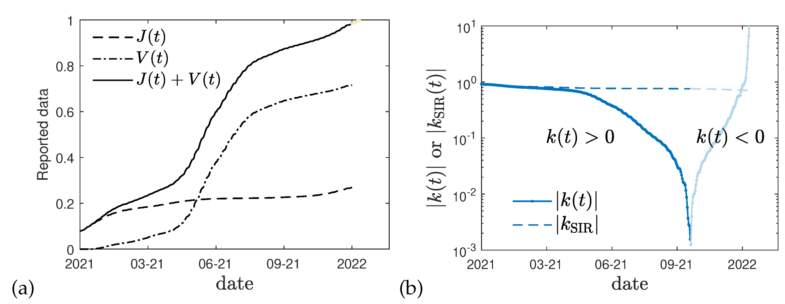
in real time, analogous to (20), is confirmed by Figure 2b where for Germany using

a_{0} = 5

day⁻¹ [38] the difference between the values of k is shown calculated with and without the effect of vaccinations. The sign change of

k (t)

visible at late times in Figure 2b may be used as an indicator, that the sum

J (t) + V (t)

(Figure 2a) approaches unity, or alternatively, that the mortality ratio

f = D (t) / J (t)

has significantly changed at the time of the divergency. This time (end of 2021) seems to coincide with the onset of the omicron wave.

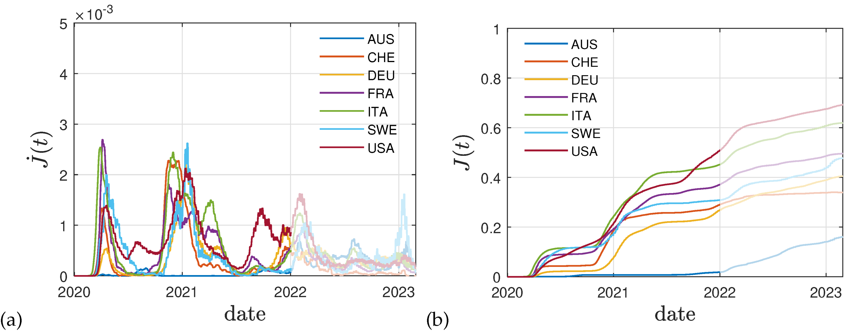
The curves are qualitatively very similar for other countries. In Figure 3a we report data for the daily number of new fatalities divided by

f = 0.005

and the size of the population, to account for the fatality rate f. This approach allows to estimate the daily population fraction of newly infected persons,

\dot{J} (t)

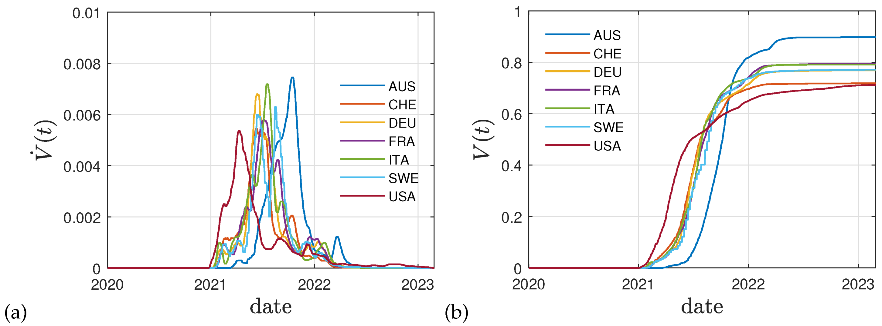
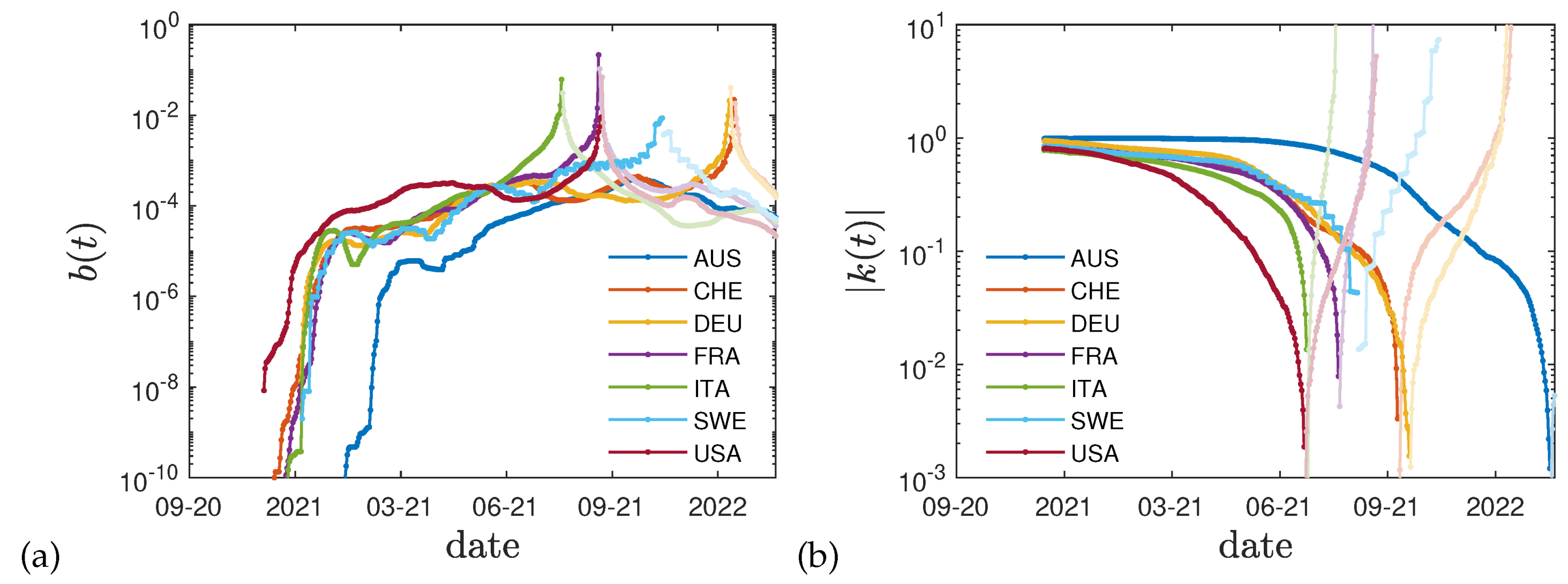
, at a much higher accuracy than using the often incomplete reported fraction of newly infected persons. The latter numbers cannot be used due to an unknown dark number of infections. Using this approach we follow previous works [38,39]. Figure 3b shows the corresponding cumulative fraction of infected persons, while Figure 4a,b display the reported vaccination data for the same eight countries: Australia (AUS), Switzerland (CHE), Germany (DEU), France (FRA), Italy (ITA), Sweden (SWE), and the United States (USA). The dimensionless rates

k (t)

and

b (t)

that we obtain using these data in Eq. (22) are given in Figure 5. As for Germany, the

k (t)

decreases with time until the fraction of vaccinated and infected persons approaches unity.

3. Cumulative Vaccination Fraction

In Figure 4 the real time history of the vaccination campaigns in selected countries is shown indicating the daily fractions of fully vaccinated persons and the total fraction summed over all vaccination campaigns. It can be seen that the shape of cumulative fraction as a function of real time and their values are of the same order.

The cumulative fraction of total vaccinated persons shown in Figure 4 can be well represented by the function

V (t) = V_{\infty} [1 - e^{- \frac{t - t_{A}}{t_{F}}}] Θ [t - t_{A}],

(23)

where

Θ

denotes the step function. The parameters

V_{\infty}, t_{A}, t_{F}

of the function (23) differ for different countries and are listed in Table 1. The starting time of the vaccination campaigns

t_{A} > t_{0}

in general is later than the starting time of the mutant wave

t_{0}

4. Conclusions

We have derived explicit expressions for the two potentially time-dependent, and dimensionless parameters

k (t)

and

b (t)

of the SIRV model in terms of measured and measurable fractions. Obtaining such parameters from reported data is an important prerequisite in the forecasting of the time-evolution of the epidemics. The time-evolution of these parameters, that are often considered constant to simplify the analysis, may be better modeled with time-evolutions from past epidemics at hand. To this end we here analyzed their time-dependency and moreover showed that using the classical SIR model, the ratio between recovery and infection rate,

k (t)

, can be highly overestimated in the presence of vaccinations. We furthermore highlighted the effect of vaccinations on the time-evolution of the

k (t)

and

b (t)

, which in turn determine the S, I, R, and V-dynamics in a straightforward fashion.

The proposed inversion method allows to infer the key parameters of the SIRV pandemic model from past Covid-19 mutant waves in terms of the well monitored cumulative fractions of new infections and vaccinations. A sign change in the temporal evolution of the ratio between recovery and infection rate can be used as a diagnostic indicator for a significant change in the mortality ratio of an ongoing mutant wave.

Author Contributions

Conceptualization, R.S.; methodology, R.S., M.K.; software, M.K.; writing—original draft preparation, R.S.; writing—review and editing, R.S., M.K.; visualization, M.K.; All authors have read and agreed to the published version of the manuscript.

Funding

This research received no external funding

Informed Consent Statement

Not applicable.

Data Availability Statement

The raw, real-time data used in this study has been retrieved from [40].

Conflicts of Interest

The authors declare no conflict of interest.

References

Schlickeiser, R.; Kröger, M. Analytical modeling of the temporal evolution of epidemics outbreaks accounting for vaccinations. Physics 2021, 3, 386–426. [Google Scholar] [CrossRef]
Babaei, N.A.; Ozer, T. On exact integrability of a Covid-19 model: SIRV. Math. Meth. Appl. Sci. 2023. [Google Scholar] [CrossRef]
Rifhat, R.; Teng, Z.; Wang, C. Extinction and persistence of a stochastic SIRV epidemic model with nonlinear incidence rate. Adv. Diff. Eqs. 2021, 2021, 200. [Google Scholar] [CrossRef]
Ameen, I.; Baleanu, D.; Ali, H.M. An efficient algorithm for solving the fractional optimal control of SIRV epidemic model with a combination of vaccination and treatment. Chaos Solit. Fract. 2020, 137, 109892. [Google Scholar] [CrossRef]
Oke, M.O.; Ogunmiloro, O.M.; Akinwumi, C.T.; Raji, R.A. Mathematical Modeling and Stability Analysis of a SIRV Epidemic Model with Non-linear Force of Infection and Treatment. Commun. Math. Appl. 2019, 10, 717–731. [Google Scholar] [CrossRef]
Kermack, W.O.; McKendrick, A.G. A contribution to the mathematical theory of epidemics. Proc. R. Soc. A 1927, 115, 700. [Google Scholar] [CrossRef]
Kendall, D.G. Deterministic and stochastic epidemics in closed populations. Proc. Third Berkeley Symp. on Math. Statist. and Prob. 1956, 4, 149. [Google Scholar] [CrossRef]
Postnikov, E.B. Estimation of Covid-19 dynamics “on a back-of-envelope?: Does the simplest SIR model provide quantitative parameters and predictions? Chaos Solit. Fract. 2020, 135, 109841. [Google Scholar] [CrossRef]
Cooper, I.; Mondal, A.; Antonopoulos, C.G. A SIR model assumption for the spread of Covid-19 in different communities. Chaos Solit. Fract. 2020, 139. [Google Scholar] [CrossRef]
Hespanha, J.P.; Chinchilla, R.; Costa, R.R.; Erdal, M.K.; Yang, G. Forecasting Covid-19 cases based on a parameter-varying stochastic SIR model. Annu. Rev. Control 2021, 51, 460–476. [Google Scholar] [CrossRef]
Annas, S.; Pratama, M.I.; Rifandi, M.; Sanusi, W.; Side, S. Stability analysis and numerical simulation of SEIR model for pandemic Covid-19 spread in Indonesia. Chaos Solit. Fract. 2020, 139, 110072. [Google Scholar] [CrossRef]
Hou, C.; Chen, J.; Zhou, Y.; Hua, L.; Yuan, J.; He, S.; Guo, Y.; Zhang, S.; Jia, Q.; Zhao, C.; et al. The effectiveness of quarantine of Wuhan city against the Corona Virus Disease 2019 (Covid-19): A well-mixed SEIR model analysis. J. Med. Virol. 2020, 92, 841–848. [Google Scholar] [CrossRef] [PubMed]
Yang, Z.; Zeng, Z.; Wang, K.; Wong, S.S.; Liang, W.; Zanin, M.; Liu, P.; Cao, X.; Gao, Z.; Mai, Z.; et al. Modified SEIR and AI prediction of the epidemics trend of Covid-19 in China under public health interventions. J. Thorac. Dis. 2020, 12, 165+. [Google Scholar] [CrossRef] [PubMed]
He, S.; Peng, Y.; Sun, K. SEIR modeling of the Covid-19 and its dynamics. Nonlin. Dyn. 2020, 101, 1667–1680. [Google Scholar] [CrossRef]
Rezapour, S.; Mohammadi, H.; Samei, M.E. SEIR epidemic model for Covid-19 transmission by Caputo derivative of fractional order. Adv. Diff. Eqs. 2020, 2020, 490. [Google Scholar] [CrossRef]
Ghostine, R.; Gharamti, M.; Hassrouny, S.; Hoteit, I. An Extended SEIR Model with Vaccination for Forecasting the Covid-19 Pandemic in Saudi Arabia Using an Ensemble Kalman Filter. Math. 2021, 9, 636. [Google Scholar] [CrossRef]
Berger, D.; Herkenhoff, K.; Huang, C.; Mongey, S. Testing and reopening in an SEIR model. Rev. Econ. Dyn. 2022, 43, 1–21. [Google Scholar] [CrossRef]
Engbert, R.; Rabe, M.M.; Kliegl, R.; Reich, S. Sequential Data Assimilation of the Stochastic SEIR Epidemic Model for Regional Covid-19 Dynamics. Bull. Math. Biol. 2021, 83, 1. [Google Scholar] [CrossRef] [PubMed]
Bentout, S.; Chen, Y.; Djilali, S. Global Dynamics of an SEIR Model with Two Age Structures and a Nonlinear Incidence. Acta Appl. Math. 2021, 171, 7. [Google Scholar] [CrossRef]
Carcione, J.M.; Santos, J.E.; Bagaini, C.; Ba, J. A Simulation of a Covid-19 Epidemic Based on a Deterministic SEIR Model. Front. Publ. Health 2020, 8, 230. [Google Scholar] [CrossRef]
Nabti, A.; Ghanbari, B. Global stability analysis of a fractional SVEIR epidemic model. Math. Meth. Appl. Sci. 2021, 44, 8577–8597. [Google Scholar] [CrossRef]
Lopez, L.; Rodo, X. A modified SEIR model to predict the Covid-19 outbreak in Spain and Italy: Simulating control scenarios and multi-scale epidemics. Results Phys. 2021, 21, 103746. [Google Scholar] [CrossRef] [PubMed]
Korolev, I. Identification and estimation of the SEIRD epidemic model for Covid-19. J. Econom. 2021, 220, 63–85. [Google Scholar] [CrossRef] [PubMed]
Jahanshahi, H.; Munoz-Pacheco, J.M.; Bekiros, S.; Alotaibi, N.D. A fractional-order SIRD model with time-dependent memory indexes for encompassing the multi-fractional characteristics of the Covid-19. Chaos Solit. Fract. 2021, 143, 110632. [Google Scholar] [CrossRef]
Nisar, K.S.; Ahmad, S.; Ullah, A.; Shah, K.; Alrabaiah, H.; Arfan, M. Mathematical analysis of SIRD model of Covid-19 with Caputo fractional derivative based on real data. Results Phys. 2021, 21, 103772. [Google Scholar] [CrossRef]
Faruk, O.; Kar, S. A Data Driven Analysis and Forecast of Covid-19 Dynamics during the Third Wave Using SIRD Model in Bangladesh. Covid 2021, 1, 503–517. [Google Scholar] [CrossRef]
Rajasekar, S.P.; Pitchaimani, M. Ergodic stationary distribution and extinction of a stochastic SIRS epidemic model with logistic growth and nonlinear incidence. Appl. Math. Comput. 2020, 377, 125143. [Google Scholar] [CrossRef]
Hu, H.; Yuan, X.; Huang, L.; Huang, C. Global dynamics of an SIRS model with demographics and transfer from infectious to susceptible on heterogeneous networks. Math. Biosci. Eng. 2019, 16, 5729–5749. [Google Scholar] [CrossRef] [PubMed]
Keeling, M.J.; Rohani, P. Modeling Infectious Diseases in Humans and Animals; Princeton University Press, Princeton, USA, 2008. [CrossRef]
Estrada, E. Covid-19 and Sars-Cov-2, Modeling the present, looking at the future. Phys. Rep. 2020, 869, 1. [Google Scholar] [CrossRef]
Lopez, L.; Rodo, X. The end of social confinement and Covid-19 re-emergence risk. Nat. Human Behav. 2020, 4, 746. [Google Scholar] [CrossRef]
Miller, I.F.; Becker, A.D.; Grenfell, B.T.; Metcalf, C.J.E. Disease and healthcare burden of Covid-19 in the United States. Nat. Med. 2020, 26, 1212+. [Google Scholar] [CrossRef]
Reiner, Jr., R. C.; Barber, R.M.; Collins, J.K.; Zheng, P.; Adolph, C.; Albright, J.; Antony, C.M.; Aravkin, A.Y.; Bachmeier, S.D.; Bang-Jensen, B.; et al. Modeling Covid-19 scenarios for the United States. Nat. Med. 2021, 27, 94+. [Google Scholar] [CrossRef]
Linka, K.; Peirlinck, M.; Sahli Costabal, F.; Kuhl, E. Outbreak dynamics of Covid-19 in Europe and the effect of travel restrictions. Comp. Meth. Biomech. Biomed. Eng. 2020, 23, 710–717. [Google Scholar] [CrossRef] [PubMed]
Filindassi, V.; Pedrini, C.; Sabadini, C.; Duradoni, M.; Guazzini, A. Impact of Covid-19 First Wave on Psychological and Psychosocial Dimensions: A Systematic Review. Covid 2022, 2, 273–340. [Google Scholar] [CrossRef]
Schlickeiser, R.; Kröger, M. Determination of a key pandemic parameter of the SIR-epidemic model from past Covid-19 mutant waves and its variation for the validity of the Gaussian evolution. Physics 2023, 5, 205–214. [Google Scholar] [CrossRef]
Schlickeiser, R.; Kröger, M. Analytical solution of the SIR-model for the temporal evolution of epidemics: Part B. Semi-time case. J. Phys. A 2021, 54, 175601. [Google Scholar] [CrossRef]
Schlickeiser, R.; Kröger, M. Reasonable limiting of 7-day incidence per hundred thousand value and herd immunization in Germany and other countries. Covid 2021, 1, 130–136. [Google Scholar] [CrossRef]
Schüttler, J.; Schlickeiser, R.; Schlickeiser, F.; Kröger, M. Covid-19 predictions using a Gauss model, based on data from April 2. Physics 2020, 2, 197. [Google Scholar] [CrossRef]
Dong, E.; Du, H.; Gardner, L. An interactive web-based dashboard to track Covid-19 in real time. Lancet Infect. Dis. 2020, 20, 533–534. [Google Scholar] [CrossRef]

Figure 1. Solution to the (a) SIR and (b) SIRV models versus reduced time

τ

for

k (τ) = 0.5 + 0.2 tanh [0.05 (τ - 30)]

η = 10^{- 8}

, and

b (τ) = 0

and

b (τ) = 0.01

in (a) and (b), respectively. Shown are

S (τ)

I (τ)

R (τ)

V (τ)

as well as

j (τ) = S (τ) I (τ)

. (c) Assuming that the data in (b) had been measured,

k (τ)

and

b (τ)

are correctly reconstructed from Eqs. (18) and (16). For comparison we show

k_{SIR} (τ)

obtained from Eq. (19).

Figure 1. Solution to the (a) SIR and (b) SIRV models versus reduced time

τ

for

k (τ) = 0.5 + 0.2 tanh [0.05 (τ - 30)]

η = 10^{- 8}

, and

b (τ) = 0

and

b (τ) = 0.01

in (a) and (b), respectively. Shown are

S (τ)

I (τ)

R (τ)

V (τ)

as well as

j (τ) = S (τ) I (τ)

. (c) Assuming that the data in (b) had been measured,

k (τ)

and

b (τ)

are correctly reconstructed from Eqs. (18) and (16). For comparison we show

k_{SIR} (τ)

obtained from Eq. (19).

Figure 2. (a) Reported data for Germany for the estimated cumulative fraction

I (t) = 200 D (t)

of infected people, where

D (t)

is the reported cumulative fraction of fatalities, and the cumulative fraction of vaccinated persons,

V (t)

, as well as their sum. We here assume that vaccinated and infected fractions belong to disjunct compartments, the SIRV model therefore breaks down as soon as the reported

I (t) + V (t)

exceeds unity, manifested by a sign change of

k (t)

. (b) Ratios

k (t)

(solid) and

k_{SIR} (t)

(dashed) according to Eq. (22) with and without

V (t)

, respectively.

Figure 2. (a) Reported data for Germany for the estimated cumulative fraction

I (t) = 200 D (t)

of infected people, where

D (t)

is the reported cumulative fraction of fatalities, and the cumulative fraction of vaccinated persons,

V (t)

, as well as their sum. We here assume that vaccinated and infected fractions belong to disjunct compartments, the SIRV model therefore breaks down as soon as the reported

I (t) + V (t)

exceeds unity, manifested by a sign change of

k (t)

. (b) Ratios

k (t)

(solid) and

k_{SIR} (t)

(dashed) according to Eq. (22) with and without

V (t)

, respectively.

Figure 3. (a) Daily fraction

\dot{J} (t)

and (b) cumulative fraction

J (t)

of infected persons in Australia (AUS), Switzerland (CHE), Germany (DEU), France (FRA), Italy (ITA), Sweden (SWE) and the United States (USA). Up to the end of 2021, the number of truly infected persons is estimated from the number of fatalities, using a fatality rate of

0.005

. Afterwards, due to a not precisely known change of the fatality rate, the estimated

\dot{J} (t)

is not considered in this work.

Figure 3. (a) Daily fraction

\dot{J} (t)

and (b) cumulative fraction

J (t)

0.005

. Afterwards, due to a not precisely known change of the fatality rate, the estimated

\dot{J} (t)

is not considered in this work.

Figure 4. (a) Daily fraction and (b) cumulative fraction of fully vaccinated persons in Australia (AUS), Switzerland (CHE), Germany (DEU), France (FRA), Italy (ITA), Sweden (SWE) and the United States (USA).

Figure 5. Rates

b (t)

and

k (t)

evaluated using Eq. (22) and the data shown in Figure 3 and Figure 4. As in Figure 2, regimes with

k (t) < 0

, here also

b (t)

, are indicated by light color.

Figure 5. Rates

b (t)

and

k (t)

evaluated using Eq. (22) and the data shown in Figure 3 and Figure 4. As in Figure 2, regimes with

k (t) < 0

, here also

b (t)

, are indicated by light color.

Table 1. Effective vaccination onset

t_{A}

, relaxation time

τ

, and final fraction of fully vaccinated persons

V_{\infty}

obtained using Eqs. (23) and vaccination data shown in Figure 4;

t_{A}

is specified in number of days after 2020-01-01.

Table 1. Effective vaccination onset

t_{A}

, relaxation time

τ

, and final fraction of fully vaccinated persons

V_{\infty}

obtained using Eqs. (23) and vaccination data shown in Figure 4;

t_{A}

is specified in number of days after 2020-01-01.

Country	$α_{3}$ code	$t_{A}$	$τ$	$V_{\infty}$
Australia	AUS	570	78 days	0.90
Switzerland	CHE	479	86 days	0.72
Germany	DEU	491	83 days	0.76
France	FRA	494	92 days	0.80
Italy	ITA	492	88 days	0.79
Sweden	SWE	503	85 days	0.77
United States	USA	407	122 days	0.70

Disclaimer/Publisher’s Note: The statements, opinions and data contained in all publications are solely those of the individual author(s) and contributor(s) and not of MDPI and/or the editor(s). MDPI and/or the editor(s) disclaim responsibility for any injury to people or property resulting from any ideas, methods, instructions or products referred to in the content.

© 2023 by the authors. Licensee MDPI, Basel, Switzerland. This article is an open access article distributed under the terms and conditions of the Creative Commons Attribution (CC BY) license (http://creativecommons.org/licenses/by/4.0/).

Copyright: This open access article is published under a Creative Commons CC BY 4.0 license, which permit the free download, distribution, and reuse, provided that the author and preprint are cited in any reuse.

MDPI Initiatives

Important Links

Choose an area of interest and we will send you notifications of new preprints at your preferred frequency.

Disclaimer

Key Epidemic Parameters of the SIRV-Model Determined from Past COVID-19 Mutant Waves

Abstract

1. Introduction

2. SIRV Model

2.1. Starting Equations

2.2. Key Parameter

2.3. Comparison with the SIR Model Limit

2.4. Real Time Dependence

3. Cumulative Vaccination Fraction

4. Conclusions

Author Contributions

Funding

Informed Consent Statement

Data Availability Statement

Conflicts of Interest

References

MDPI Initiatives

Important Links

Subscribe