Proportional Equation and Multiplicative Superposition: New Way to Understand Reality

Preprint

Article

Proportional Equation and Multiplicative Superposition: New Way to Understand Reality

Altmetrics

Downloads

141

Views

Comments

Seong-Dong Kim^*

This version is not peer-reviewed

Submitted:

31 March 2023

Posted:

31 March 2023

You are already at the latest version

Alerts

Abstract

We still do not have satisfactory answers about the inflationary and accelerating expansions of the universe, the missing mass problem, and the origins of the four fundamental forces and the quantum phenomena. Here, we introduce a new model of matter and space and a postulate on a constant of motion, and then show that an equation of motion derived from the constant of motion could provide new understandings of the above problems. For example, we show that there is a natural inflation scenario and that the co-moving distance to the closest accelerating supernova is clearly given as $c/(\sqrt{3} H)$ ($\sim$8.1 billion ly). In addition, we show that, in a system including a proton and an electron, the equation of motion has eight acceleration terms, some of which are suspected to be responsible for the four fundamental forces and the galaxy rotation anomaly. From further discussion, we conjecture that in order to understand the gravitational and strong interactions and the quantum phenomena, it is necessary to consider the expansion of the universe. The lensing mass distribution is explained, based on another postulate on a method of representing superposition.

Keywords:

Subject: Physical Sciences - Theoretical Physics

1. Introduction

We believe that, in the universe, there is a quantitative order that can be explained by physics. Where does such a quantitative order come from? Regardless of whether it is right or not, an answer to this question relies on what model of space we select, because all physical phenomena occur in space. Roughly speaking, there have been two types of space models: a) 0-based models interpreting the space as nothing to which the number of zero can be assigned and b) 1-based models opposing this interpretation. The currently most-widely accepted model is the 0-based model called the atomism, in which the space is interpreted as an empty (i.e., zero-assigned) void between atoms. However, in the case that zero, the very special number, is assigned to the space, the space itself can no longer be treated as a quantitative entity and is completely forgotten in a theorization process. Only by assuming additional constraints, such as the conservation laws, the least action principle, or the Einstein field equation (EFE), the space could be incorporated into theories. Nevertheless, this process enables the space to have some quantitative properties that are limitedly given by such constraints, at best.

Despite the great achievements accomplished based on the atomism, there are still difficulties in understanding the inflationary and accelerating expansions of the universe[1,2,3], the missing mass problem[4,5,6,7,8], and the origins of the four fundamental forces and the quantum phenomena[9,10]. Thus, in this article, we will consider a new 1-based space model, in which the whole universe is regarded as a single kind of real entity itself (hereinafter, "Mach fluid") completely filling a 3-dimensional space and the apparent difference between matter and space is regarded as a consequence of a difference in (1-dimensional) density of the Mach fluid (hereinafter, “(1D) Mach density”). It should be noted that, in this model, the space has inherent quantitative properties, not properties limitedly given by the constraints. In particular, the reader should pay attention to the fact that, due to such inherent quantitative properties, the Mach density of the space can be changed not only in space, but also in time. We will show that the temporal variation of the 1D Mach density is related to most of the above problems.

Before we go on, let us first define some terms to be used in this article. Two observers, Murphy and Cooper, will be mentioned in this article. Murphy is an actual observer (e.g., in the laboratory) in the present epoch of the expanding universe, observing a target object (hereinafter, “TARS”). Cooper is an imaginary observer who is located at the same point in spacetime as TARS, is instantaneously at rest with respect to Murphy, not to TARS, and is accelerated with the same acceleration as TARS. It is obvious that the above requirements for Cooper cannot be satisfied by a single observer, and this means that Cooper should be interpreted as a theoretical element for parameterization or a group of observers. TARS, i.e., the target object, may be an electron, a positron, a star, or a galaxy, depending on what system we select, but in a sense, it corresponds to a free-falling observer in the general theory of relativity. In this article, we will pay attention to physical descriptions made by Cooper, not by TARS (i.e., the free-falling observer). This means that we will develop our theory in a manner similar, but different, to the general theory of relativity (see Appendix A and Appendix B). A distribution factor

Λ (r, t)

, which is a scalar function defined at every point

(r, t)

in spacetime, will be used to represent a variation in space and time of the 1D Mach density. It should be remembered that

Λ (r, t)

should be a non-negative real number (hereinafter, “numerical restriction”) and has an observer-independent property, because the Mach fluid is supposed as the real entity.

The article is organized as follows. In Sec. 2, we introduce three postulates and derive two equations of motion, Eqs. (8) and (9), which are valid for Cooper and Murphy, respectively. In the first postulate, we propose a mathematical way of expressing the superposition in a many body system. In the second postulate, we introduce a quantity,

ε

, which will be used as a constant of motion for Cooper. In the third postulate, we introduce calibration factors, which define ratios between spatial/temporal lengths in Cooper and Murphy’s frames and are used as parts of the metric tensor. The equation of motion, Eq. (8), which is valid for Cooper, is derived from the constant of motion

ε

, and the equation of motion, Eq. (9), which is valid for Murphy, is obtained by projecting Eq. (8) onto the Murphy’s frame. The calibration factors in the postulate 3 are used for this projection. In Sec. 3.1, a system of

Λ = Λ (t)

will be discussed to explain our results on the inflationary and accelerating expansions of the universe. In Sec. 3.2, a spherically symmetric static system will be discussed to determine a distribution factor

Λ (r)

producing an inverse square field. In Sec. 3.3, we show that the constant of motion,

ε

, is a quantity associated with the energy conservation law. In Sec. 3.4, we define a pair of distribution factors,

Λ_{\pm} (r)

, for proton and electron. In Sec. 3.5, we discuss implications of the distribution factors

Λ_{\pm} (r)

. In Sec. 3.6, we briefly explain how to understand the quantum phenomena in our approach and then derive an equation resembling the Schrödinger’s equation. In Sec. 3.7, we explain how to understand the lensing mass distribution, which is one of observations associated with the missing mass problem, based on the first postulate. In Sec. 3.8, we show that, in the case that the Mach density is changed with time (e.g., by the expansion of the universe), the electric force can be split into eight distinct forces. In Sec. 3.9, we review interesting and perplexing aspects in the results of Sec. 3.8. In Sec. 3.10, we mention our vague ideas to alleviate the perplexing problems. In Sec. 4, we propose experiments to test our approach.

2. Theory

In this article,

d X^{0} (= d p)

and

d X^{i}

will be used to represent temporal and spatial lengths in Cooper’s frame, and

d x^{0} (= d t)

and

d x^{i}

(

i = 1, 2, 3

) will be used to represent those in Murphy’s frame. A calibration factor

h_{μ} (r, t)

will be used to define a ratio between the lengths

d X^{μ}

and

d x^{μ}

, where

r

is a position of TARS or Cooper at time t in Murphy’s frame and

μ = 0, 1, 2, 3

. Retarded time is not considered in this article, for simplicity.

2.1. Postulate 1 - Mach Principle

The superposition in a many body system is represented by multiplication of distribution factors of objects constituting the system, not by summation, as follows:

Λ (r, t) = Λ_{M} (r, t) \prod_{i = 1}^{n} Λ_{i} (r - r_{i}, t),

(1)

where n is the number of source objects (i.e., matters) constituting a chosen source system,

Λ_{i}

is a distribution factor of an i-th source object whose characteristic point (e.g., center) is located at

r_{i}

, and

Λ_{M}

is a factor representing contributions from all other objects in the universe, except the chosen source system, on the distribution factor

Λ

Here,

Λ (r, t)

in the left-hand side can be understood as a distribution factor representing a background space for TARS, and in the same context,

Λ_{M} (r, t)

can be understood as a distribution factor representing a background space (hereinafter, ‘Machian space’) for the chosen source system. In this article, a term ’Machian objects’ will be used to refer to all other objects in the universe, except the chosen source system.

2.2. Postulate 2 - Constant of Motion

For an observer (e.g., Cooper) at the same point in spacetime as TARS, the following proportional equation is valid.

\begin{matrix} ε (X^{i}, V, p) & \equiv ψ_{0} \frac{γ (V)}{Λ (X^{i}, p)} = constant, and \end{matrix}

(2)

\begin{matrix} γ (V) & = {(1 - \frac{V^{2}}{c^{2}})}^{- 1 / 2}, \end{matrix}

(3)

where

V

is a three velocity of TARS measured by Cooper: that is,

V = \sum_{i = 1, 2, 3} \frac{d X^{i}}{d p} {\hat{X}}_{i}

and

{\hat{X}}_{i}

is a three basis vector in Cooper’s frame. The equation (3) is the Lorentz factor, which is given as a function of the velocity

V

. It should be noted that Eq. (2) is valid for Cooper, not for Murphy, and thus, that the quantity

ε

in Eq. (2) serves as a constant of motion for only Cooper. A further detailed comment on the postulate 2 can be found in Appendix A. Meantime, in some topics, we will consider a case, in which TARS and Cooper are located at the same point in spacetime as Murphy (hereinafter, ‘coincidence condition’). Note that, under such a coincidence condition,

V

becomes equal to a velocity,

v = \sum_{i = 1, 2, 3} \frac{d x^{i}}{d t} {\hat{x}}_{i}

, measured by Murphy; that is, Cooper’s description becomes equal to Murphy’s description. The quantity

ψ_{0}

is introduced to represent a physical quantity associated with TARS, and it will be regarded as a constant unless otherwise noted.

2.3. Postulate 3 - Metric Tensor

Calibration factors

h_{μ}

are given as follows:

\begin{matrix} d X^{i} & = h_{i} (r, t) d x^{i}, and \end{matrix}

(4)

\begin{matrix} c d p & = c d t / h_{0} (r, t), \end{matrix}

(5)

where c is the speed of light, and for a spherically symmetric system, the calibration factors are given as follows:

h_{0} = h_{1} = Λ (r, t), h_{2} = r, h_{3} = r \sin θ

(6)

In this article, we will restrict our attention to only three systems of

Λ (t)

Λ (r)

, and

Λ (r, t)

. The gist of the postulate 3 is that, in such three systems, the metric tensor can be diagonalized and the diagonalized components can be expressed in terms of the distribution factor, as stated by Eq. (6). One might think that the postulate 3 is reasonable, but in a sense, it is true that it is not rigorous or complete. A further comment on this issue can be found in Appendix B.

2.4. Equation of Motion

Using

\partial γ / \partial V^{i} = (γ^{3} / c^{2}) V^{i}

and

V^{2} = V \cdot V

, the total derivative of the constant

ε

in Eq. (2) with respect to Cooper’s time p gives:

0 = - \frac{c^{2}}{μ γ^{2}} V \cdot (\frac{\partial μ}{\partial p} \frac{V}{V^{2}} + \tilde{\nabla} μ - \frac{μ γ^{2}}{c^{2}} A),

(7)

where

μ = Λ (r, t) / ψ_{0}, A = d V / d p

, and

\tilde{\nabla} μ

is a gradient operator in Cooper’s frame (i.e.,

\frac{\partial μ}{\partial X^{i}} {\hat{X}}_{i}

). In general,

V

is not a zero vector, so Eq. (7) is valid only when the bracketed quantity is equal to

0

and/or is perpendicular to

V

. In the former case, we can obtain the following equation (8) from Eq. (7). For the time being, we will continue our discussion on the basis of Eq. (8), but the reader should remember that Eq. (7), not Eq. (8), is the equation valid for general cases.

A = \frac{c^{2}}{μ γ^{2}} (\frac{\partial μ}{\partial p} \frac{V}{V^{2}} + \tilde{\nabla} μ) .

(8)

According to the postulate 2, the trajectory of TARS described by Eq. (8) is valid for Cooper, but not for Murphy in general. This means that if Murphy uses Eq. (8) as it is, she will observe an anomalous result. This is because Murphy’s ruler and clock are not calibrated to have validity at a region of Murphy, not TARS, and this is the gist of the postulate 2 (see Appendix B). According to the postulate 3, such a calibration can be achieved by using Eqs. (4) and (5). For example, by transforming Eq. (8) to Murphy’s frame using Eqs. (4) and (5)[11], we obtain the equation of motion, which is valid for Murphy, as follows (see Appendix C):

\begin{matrix} \frac{d^{2} x^{k}}{d t^{2}} = \frac{c^{2}}{γ^{2}} [(\frac{1}{μ} \frac{\partial μ}{\partial t}) \frac{v^{k}}{V^{2}} + \frac{1}{h_{0}^{2} h_{k}^{2}} (\frac{1}{μ} \frac{\partial μ}{\partial x^{k}})] - \frac{d x^{k}}{d t} (\frac{1}{h_{0}} \frac{d h_{0}}{d t}) - Γ_{j β}^{k} \frac{d x^{j}}{d t} \frac{d x^{β}}{d t}, \end{matrix}

(9)

where

Γ_{j β}^{k} = \frac{\partial^{2} X^{i}}{\partial x^{j} \partial x^{β}} \frac{\partial x^{k}}{\partial X^{i}}

and the repeated indices, except the calibration factors

h_{k}

, mean the summation. Rewriting Eq. (9) using Eq. (6), we can obtain the equations of motion for a spherically symmetric system, as follows (see Appendix D):

\begin{matrix} a_{r} = [\frac{c^{2}}{V^{2}} - 3] [\frac{1}{Λ} \frac{\partial Λ}{\partial t} \dot{r} + \frac{V^{2}}{Λ^{4}} \frac{1}{Λ} \frac{\partial Λ}{\partial r}] + [\frac{2}{Λ} \frac{\partial Λ}{\partial r} + \frac{1}{r}] \frac{r^{2} {\dot{Ω}}^{2}}{Λ^{2}}, \end{matrix}

(10)

\begin{matrix} a_{θ} = [\frac{c^{2}}{V^{2}} - 2] \frac{1}{Λ} \frac{\partial Λ}{\partial t} \dot{θ} - \frac{1}{Λ} \frac{\partial Λ}{\partial r} \dot{r} \dot{θ} - \frac{2}{r} \dot{r} \dot{θ} + \cos θ \sin θ {\dot{φ}}^{2}, and \end{matrix}

(11)

\begin{matrix} a_{φ} = [\frac{c^{2}}{V^{2}} - 2] \frac{1}{Λ} \frac{\partial Λ}{\partial t} \dot{φ} - \frac{1}{Λ} \frac{\partial Λ}{\partial r} \dot{r} \dot{φ} - \frac{2}{r} \dot{r} \dot{φ} - 2 \cot θ \dot{θ} \dot{φ}, \end{matrix}

(12)

where

V^{2} = Λ^{4} ({\dot{r}}^{2} + r^{2} {\dot{Ω}}^{2} / Λ^{2})

and

\dot{Ω} = \dot{θ} + \sin θ \dot{φ}

3. Application and Discussion

3.1. System of $Λ = Λ (t)$ : Inflationary and Accelerating Expansions of the Universe

Here, we discuss the inflationary and accelerating expansions of the universe, based on Eq. (10). For brevity, we will restrict our attention to a one-dimensional motion of TARS, under the cosmological principle (i.e.,

\partial_{x} Λ = 0

). Then, we can describe this system using the position-independent distribution factor

Λ = Λ (t)

and can neglect any angular component in Eq. (10). That is, it is enough to consider only a difference in

Λ (t)

between epochs, in which Cooper and Murphy live. To take such a difference into consideration, suppose that Murphy and Cooper are two observers in the present and past epochs,

t_{0}

and

t < t_{0}

, respectively. Then, we can rewrite Eq. (10), as follows:

\ddot{d} (t) = (\frac{1}{Λ {(t)}^{4}} \frac{c^{2}}{\dot{d} {(t)}^{2}} - 3) (\frac{1}{Λ (t)} \frac{\partial Λ (t)}{\partial t}) \dot{d} (t),

(13)

where

\dot{d} (t)

is a projection speed that is obtained by projecting a one-dimensional speed of TARS, measured by Cooper in the past epoch t, onto the Murphy’s frame in the present epoch

t_{0}

Meanwhile, in this system of

Λ = Λ (t)

, we can freely choose the positions of Cooper and TARS, without the constraint of the sameness in space, although Cooper and TARS should be still chosen to be in the same epoch. Thus, we can define a distance,

d (t)

, from Cooper to TARS, even when TARS is very far from Cooper. However, if, as stated by the Hubble’s law, the expansion rate of the universe (i.e., the speed

\dot{d} (t)

) depends on the distance

d (t)

, the acceleration

\ddot{d} (t)

in the above equation should also vary depending on a distance

d (t)

to a chosen object (i.e., TARS). We think that the accelerating expansion of the universe can be explained based on this property of the acceleration

\ddot{d} (t)

In detail, let us introduce the scale factor

S (t) = d (t) / d_{c}

, where

d_{c}

is a co-moving distance between Cooper and TARS (e.g., a distant supernova). Owing to the cosmological principle, we can freely place Cooper at the same position as Murphy, and in this case, Murphy has the same co-moving distance. By definition, the distribution factor is inversely proportional to the scale factor: that is,

Λ (t) \propto 1 / S (t)

. Using this, we can define a deceleration parameter

q (t)

, from Eq. (13), and a time-dependent Hubble parameter

H (t)

, as follows:

\begin{matrix} q (t) & = - \frac{S (t) \ddot{S} (t)}{\dot{S {(t)}^{2}}} \propto (\frac{S {(t)}^{2} c^{2}}{H {(t)}^{2} d_{c}^{2}} - 3), and \end{matrix}

(14)

\begin{matrix} H (t) & = \frac{\dot{S} (t)}{S (t)} = - \frac{1}{Λ (t)} \frac{\partial Λ (t)}{\partial t} . \end{matrix}

(15)

It should be noted that the sign of the deceleration parameter

q (t)

relies on the co-moving distance

d_{c}

to the chosen supernova. Since, by definition,

S (t_{0}) = 1

, Eq. (14) states that if we observe a distant object farther than

c / \sqrt{3} H

, we will find a positive value of acceleration. If the Hubble parameter

H (t_{0})

at the present epoch (hereinafter,

H_{0}

) is selected as 70 km/s/Mpc[12], the co-moving distance to such a turning point is

7.6 \times 10^{25}

m or 8.1 billion ly[13]. Furthermore, Eq. (15) states that the Hubble parameter

H (t)

can vary depending on the distribution factor

Λ (t)

, and this may be a clue to the discrepancy between two Hubble parameters independently obtained from the cosmic microwave background (CMB) and supernovae observations[12].

Now, let us discuss the inflationary expansion of the universe. An expansion of the universe means that

\dot{d} > 0

and

\partial_{t} Λ (t) < 0

, and, due to the numerical restriction,

Λ (t)

should be a non-negative real number. Thus, the acceleration

\ddot{d}

in Eq. (13) can be positive, only when

\dot{d} (t) > \frac{c}{\sqrt{3}} \frac{1}{Λ {(t)}^{2}} \overset{def}{=} v_{c} (Λ) .

(16)

According to this condition, if

0 < \dot{d} < v_{c}

, there is no lasting expansion, and just a small vibration is allowed. However, if

\dot{d} > v_{c}

, the inflationary expansion or the big bang can be triggered. At the initial stage of the big bang,

Λ

would be a very large value, and this means that the inflationary expansion could be triggered by even a very small value of

\dot{d}

. The inflationary expansion would lead to a fast decrease of

Λ

and a fast increase of

\dot{d}

. Nevertheless, during this inflation era, the evolution of the universe would be substantially dominated by the decrease of

Λ^{4}

in Eq. (13), not by the increase of

{\dot{d}}^{2}

, because

Λ^{4}

would be still extremely high and

c^{2} / {\dot{d}}^{2}

would be substantially a bounded value. Thereafter, when

Λ

decreased to a sufficiently low value (e.g., roughly of the order of one), the system could be naturally escaped from the condition of Eq. (16).

Until now, we have discussed the inflationary and accelerating expansions of the universe only in terms of acceleration based on Eq. (10)). Thus, in order to see if the above results are compatible with the existing results, it is necessary to further study these topics on thermodynamics and the like.

3.2. System of $Λ = Λ (r)$ : Determining $Λ (r)$

We will here determine a distribution factor

Λ

of a source object producing an inverse square field (e.g., the electric or gravitational field). To do this, we will substitute

k / r^{2} \hat{r}

into the left-hand side (LHS) of Eq. (8), where k is

k_{e} Q

and

- G M

for the electric and gravitational fields, respectively,

k_{e}

and G are the Coulomb and Newton constants, Q and M are an electric charge and a mass of the source object, and r is the radial distance from the center of the source object. Because of

Λ = Λ (r)

, the right-hand side (RHS) of Eq. (8) has only the radial component of the gradient term. Thus, using the relation

γ = ε Λ / ψ_{0}

of Eq. (2), Eq. (8) can be written as follows:

\frac{k}{r^{2}} \hat{r} = \frac{1}{χ} \frac{c^{2}}{Λ^{3}} \frac{d Λ}{d r} \hat{r},

(17)

where

χ = ε^{2} / ψ_{0}^{2}

. The solutions of this differential equation are:

Λ (r) = \pm {[\frac{2 k χ}{c^{2}} (\frac{1}{r} - \frac{1}{r_{0}}) + \frac{1}{Λ_{0}^{2}}]}^{- 1 / 2},

(18)

where

r_{0}

is a reference position and

Λ_{0}

is a reference value of

Λ

defined at

r_{0}

. By the numerical restriction on

Λ

, the negative solution will be excluded from our discussion. If the references

r_{0}

and

Λ_{0}

are choose as ∞ and 1, respectively, the positive solution can be written as follows:

Λ (r) = {(1 + \frac{2 k χ}{r c^{2}})}^{- 1 / 2} .

(19)

Meanwhile, by the postulate 2, the formula

γ = ε Λ / ψ_{0}

and Eq. (8) are valid in only the Cooper’s frame. Thus, Eq. (17) is true under the coincidence condition. Nevertheless, due to its observer-independent property,

Λ

has the same physical meaning, regardless of who is chosen to determine it. By analogy, even when a balloon has a size varying with height, it is possible to uniquely determine the geometry of a mountain, if a specific balloon (e.g., at a specific height) is solely used. Mathematically, this means that a relationship between

Λ_{c}

and

Λ_{m}

, described by Cooper and Murphy, respectively, is given by

Λ_{c} (r, t) = c_{1} Λ_{m} (r, t)

, where

c_{1}

is a ratio specifically given based on their positions in spacetime. Here, since

c_{1}

is canceled in each term in RHS of Eq. (8), it does not affect the actual calculation. Thus, even if

Λ

is obtained under the coincidence condition, it can be validly used for in our discussion.

3.3. Physical Meanings of the Constant of Motion $ε$

Here, we will discuss the physical meanings of the constant of motion

ε

, based on the above results. Using Eqs. (2) and (19), we can obtain the following formula.

\frac{ε}{ψ_{0}} = \frac{γ}{Λ} = \sqrt{χ} = \pm {[1 - \frac{V^{2}}{c^{2}} - \frac{2 k}{r c^{2}}]}^{- 1 / 2} .

(20)

Here, we will again neglect the negative solution1 of Eq. (20). Multiplying both sides of the positive solution of Eq. (20) by

m_{0} c^{2}

and expanding the RHS in series, we find

E = \frac{1}{2} m_{0} V^{2} + \frac{k m_{0}}{r} + O (V^{4}, \frac{1}{r^{2}}),

(21)

where

E = m_{0} c^{2} (\sqrt{χ} - 1)

. This result shows that we can say that, just as

γ

is a dimensionless number associated with a relativistic kinetic energy of an object with unit mass,

ε

and

Λ

are dimensionless numbers associated with a relativistic total energy (including a rest energy,

m_{0} c^{2}

) and a relativistic potential energy, respectively, for a system of

ψ_{0} = 1

. That is, we can say that Eq. (2) or (20) is another expression of the energy conservation law.

3.4. Distribution Factors of Proton and Electron

χ = 1

and

k = - G M

, the RHS of Eq. (19) is the very factor characterizing the Schwarzschild solution[14], and thus, we can immediately construct the Schwarzschild metric from Eqs. (4), (5), (6), and (19). Moreover, we also find that, in the case of

\partial_{t} Λ = 0

, the equations of motion (10) to (12) are similar to, but slightly different from, those for the Schwarzschild system in the general relativity[15]. However, we will trace the route of

k = k_{e} Q

, instead of

k = - G M

, because one of

\partial_{t} Λ

-containing terms in Eq. (10) exhibits gravity-like behaviors, as will be described below. If this route is right, it implies that the

\partial_{t} Λ

factor (e.g., caused by the expansion of the universe), not a usually-expected

\partial_{x} Λ

factor, is responsible for the gravity.

To go this route, let us first consider the cases of

Q = \pm e

(

e = 1.602 \times 10^{- 19} C

). Then, Eq. (19) is written as follows:

Λ_{\pm} (r) = {(1 \pm \frac{2 k_{e} e χ}{r c^{2}})}^{- 1 / 2} .

(22)

The reader can find that the plotting curves of

Λ_{\pm} (r)

are asymmetric about the reference value

Λ_{0}

: i.e.,

| Λ_{-} (r) - 1 | \neq | Λ_{+} (r) - 1 |

. This is analogous to the fact that there is a difference in mass between proton and electron that have opposite electric charges. Also,

Λ_{-} (r)

has a singularity at

r_{s} = 2 k_{e} e χ / c^{2}

and has an imaginary value in the inner region (

r < r_{s}

), but

Λ_{+} (r)

does not. Considering that the numerical restriction prohibits an imaginary value of

Λ

, it looks as if an internal structure is required to prevent the imaginary value of

Λ_{-} (r)

. Furthermore, if the inverse square field is natural in the 3-dimensional space, it will be natural to regard Eq. (22) obtained therefrom as the most fundamental distribution factors (e.g., for the stable particles)2. For these reasons, we will regard

Λ_{-} (r)

and

Λ_{+} (r)

as the distribution factors of proton and electron and will interpret the electric charge (Q) and the mass (m) as numbers associated with the sign and value of the quantity

(Λ - 1)

3.5. Implications of Equation (22)

The above interpretation forces us to regard the proton or electron as a 3D ubiquitous object existing throughout the universe, not as a point-particle. Indeed, this is just the very result required by our space model. According to this picture, each object interacts with all other objects in the universe, because it has not only an observable part (i.e., matter) but also an unobservable prevailing part. Although this picture may look very weird in the classical point of view, it seems to be compatible with the quantum mechanical point of view. Rather, this picture may alleviate the fundamental difficulty in understanding the quantum phenomena, such as the wave-particle duality (especially, the self-interaction of single electrons in the double slit experiment[16]). Furthermore, this picture allows us to avoid the unnatural interpretation, which states that a 0-dimensional point particle has ’intrinsic properties’ such as mass, spin, and charge, although such an interpretation was inevitable under the existing atomism. For example, according to this picture, each object is a 3D ubiquitous structure with a very large (in fact, infinite) degree of freedom, and this allows us to correlate a number of physical properties in each object with a 3-dimensional structure given by Eq. (22), instead of relying on an unnatural expression of ’intrinsic’. In this case, it would be natural to interpret some fundamental quantities, such as mass, charge, and spin, as being related to structural stability of each particle under the cosmic-scale interaction with all other objects.

Considering the cosmic-scale interaction of each object, behaviors of each object could be completely comprehended, only when the object is described as a whole, not just an observable part (i.e., matter). In this context, it is clear that

ψ_{0}

in Eq. (2) is an oversimplified description for TARS and that such a particle-based description, which describes only the observable part of the object using a constant

ψ_{0}

, cannot be true, although it is inevitable. In order to correctly describe the motion of TARS as a whole, it would be necessary to restore

ψ_{0}

ψ (r, t)

. Although, as of now, it is unclear whether

ψ (r, t)

corresponds to the distribution factor of TARS, we will assume that such a restoration gives a correct result, and the topic of quantum mechanics below will be discussed, under this assumption.

3.6. Quantum Phenomena : Implications of Equation (7)

The reader will know that our results on the expansions of the universe are closely related to the quantity of

Λ^{- 1} \partial_{t} Λ

in Eq. (7). In a sense, such discussions are related to the collective or time-averaged behavior of

Λ^{- 1} \partial_{t} Λ

in a many body system, in that an astronomical object is made of many elementary particles. Here, we will discuss the instantaneous behaviors of

Λ^{- 1} \partial_{t} Λ

of an elementary particle. To do this, we will assume that the restoration

ψ_{0} \to ψ (r, t)

gives the more correct result, as mentioned above, and, for brevity, the source system is composed of a single object. Furthermore, we will discuss this topic under the coincidence condition, because what we want to know here is just the physical meanings of Eq. (7), not exact calculation. Using Eqs. (1) and (2) under the coincidence condition, we can rewrite Eq. (7), as follow:

(\frac{1}{Λ_{s}} \frac{\partial Λ_{s}}{\partial t} - \frac{1}{ψ} \frac{\partial ψ}{\partial t} + \frac{1}{Λ_{M}} \frac{\partial Λ_{M}}{\partial t}) = v \cdot (\frac{γ^{2}}{c^{2}} a - \frac{1}{μ} \nabla μ),

(23)

where

Λ_{s}

is a distribution factor of the source system and ∇ is the gradient operator. From Eq. (15), we know that the LHS of Eq. (23) (especially, the third term) will be affected by the expansion of the universe. In addition to an effect by such a cosmic expansion, according to Eq. (1), the first to third terms in LHS of Eq. (23) will also be affected by each of changes in position and distribution factor of the source, target (TARS), and Machian objects. For example, a change in position of any object having a non-uniform distribution factor leads to a change in the total distribution factor. This means that, in general, the LHS of Eq. (23) is neither zero nor constant: that is, there is a ceaseless fluctuation in every point of space. This fluctuation in the value of the LHS of Eq. (23) will be used as an argument to explain an aspect of the gravitational force.

Meanwhile, for some reasons, it seems that Eq. (7) or (23) is related to the quantum phenomena. For example, since this equation is a direction-independent scalar equation, it allows for a certain freedom in direction of motion of TARS, unexpected in the classical physics, as long as the motion satisfies the scalar condition given by Eq. (23) or the energy conservation required by Eq. (2) or (20). In classical physics,

v

a

, and

\nabla μ

are causally-connected vector quantities, and thus, for a free-falling object, if the LHS of Eq. (23) is zero, the cancellation of the common factor

[v \cdot]

in Eq. (23) may be allowed, as in Eq. (8). However, if the LHS of Eq. (23) is not zero as stated above, such a cancellation will not be allowed in general. This means that the scalar equation (7), not the vector equation (8), should be used to more correctly describe the universe. Furthermore, this seems to imply that the causality in direction may be an illusory notion (e.g., resulting from our experience in the macroscopic world or the collective objects) and that the difficulties in understanding the quantum phenomena may perhaps be due, at least in part, to our belief on causality in direction.

If Eq. (23) is correct, we might be able to derive the equations of quantum mechanics from Eq. (23), because the quantum mechanics gives more correct results for such a microscopic object. We can find one clue for this, from Eqs. (20) and (21). That is, changing

ψ_{0}

ψ (r, t)

, using the formula

χ = q / m_{0}

for TARS, and using the operators (i.e.,

i ℏ \partial_{t} = E

and

- i ℏ \partial_{x} = P_{x}

) for a plane wave, we can get the following equation, from Eqs. (20) and (21), under the coincidence condition.

i ℏ \frac{\partial}{\partial t} ψ (r, t) = (- \frac{ℏ^{2}}{2 m_{0}} \nabla^{2} + \frac{q}{χ} \frac{k}{r}) ψ (r, t) .

(24)

Although this equation resembles the Schrödinger’s equation[21], it is true that there are some vague aspects associated with physical meanings of

ψ

and

χ

and so further study is needed.

3.7. Missing Mass Problem: Lensing Mass Distribution

This problem is related to two different types of observations: 1) the galaxy rotation anomaly[4,5] and 2) the lensing mass distribution[6,7,8]. Here, we will first discuss the lensing mass distribution, based on the postulate 1, and then discuss the galaxy rotation anomaly in the issue [A3] of Sec. 3.9. According to the conventional (i.e., sum-based) representation of superposition, the total gravitational potential of a galaxy is expressed by

V_{G} = \sum_{i = 1}^{n} V_{i}

, where

V_{i} = - k_{i} / | r - r_{i} |

. This means that objects (e.g., stars or atoms) in the galaxy contribute independently to the total gravitational potential

V_{G}

. By contrast, according to the multiplicative representation of superposition required by the postulate 1, the total distribution factor of the galaxy is expressed by

Λ_{G} = \prod_{i = 1}^{n} Λ_{i}

, if

Λ_{M} = 1

in Eq. (1) for brevity. This implies that each object reveals its presence (i.e.,

Λ_{i}

) as a ratio to a background distribution factor made by all other objects constituting the galaxy.

Note that

(Λ_{G} - 1) c^{2} - | V_{G} | > 0

always. This means that there is a boosting effect. It should be noted that, according to our multiplicative representation, the greater the background distribution factor at a position of each object, the larger the overall boosting effect. This means that a high-

Λ

region (e.g., in the vicinity of a black hole or in a region of densely-crowded stars) serves as a boosting seed causing a significant increase of

Λ_{G}

. By contrast, for a dilute gas structure, even if it has a large total mass, a boosting effect caused thereby is negligible, because a distance between atoms is too large. This model including the boosting effect allows us to explain why the lensing effect in the bullet cluster[6] is overlapped with the galaxies, not with the dilute hot gas, and probably why there is a large difference in dark matter amount between Dragonfly 44 and NGC 1052-DF2[7,8] (if they have a large difference in compactness).

3.8. System of $Λ = Λ (r, t)$ : Eight Separate Forces

We now calculate a radial acceleration (i.e., Eq. (10)), which is exerted on one electron or positron located near one proton, in the present epoch in the expanding universe. Note that, in our 1-based model, this system should be treated as a three-body system including the Machian space, in addition to proton and electron.

To calculate Eq. (10), we should know

Λ^{- 1} \partial_{r} Λ, Λ^{- 1} \partial_{t} Λ

, and

Λ^{2}

. To simplify this calculation, let us place the source object (i.e., proton) at the origin of a spherical coordinate system. Then, Eq. (1) for this system can be written as

Λ (r, t) = Λ_{M} (r, t) Λ_{p} (r, t)

, where

Λ_{M} (r, t)

and

Λ_{p} (r, t)

are time-dependent distribution factors of the Machian space and the proton.

Next, to reduce the difficulty in calculating Eq. (10), we will make some assumptions on

Λ_{M}

and

Λ_{p}

. First, suppose that each of

Λ_{M}

and

Λ_{p}

can be separated into spatial and temporal parts (i.e.,

Λ_{M} = S_{M} (r) T_{M} (t)

and

Λ_{p} = S_{p} (r) T_{p} (t)

). Second, suppose that the spatial parts of the Machian space and the proton are homogeneous and spherically symmetric, respectively (i.e.,

S_{M} (r) = 1

and

S_{p} (r) = S_{p} (r)

). Then, we find

Λ = T_{M} (t) T_{p} (t) S_{p} (r)

and

Λ^{- 1} \partial_{r} Λ = S_{p}^{- 1} \partial_{r} S_{p}

Our next goal is to determine

Λ^{- 1} \partial_{t} Λ

. From Eq. (15), we know

T_{M}^{- 1} \partial_{t} T_{M} = - H_{0}

under the cosmological principle, but strictly speaking, we don’t know instantaneous values of

T_{M}^{- 1} \partial_{t} T_{M}

and

T_{p}^{- 1} \partial_{t} T_{p}

. Thus, let us suppose that

Λ^{- 1} \partial_{t} Λ

is in proportion to the Hubble constant

H_{0}

(i.e.,

Λ^{- 1} \partial_{t} Λ = α H_{0}

). Here, it should be noted that, due to the ceaselessly changing property of the LHS of Eq. (23) stated above, the parameter

α

should also be a ceaselessly changing value.

Lastly, in the present epoch,

T_{M} (t_{0}) = T_{p} (t_{0}) = 1

, and thus, we can say that

{Λ (r, t) |}_{t = t_{0}} = S_{p} (r)

. The spatial part of the source system,

S_{p} (r)

, can be expressed using

Λ_{-} (r)

of Eq. (22), and thus, the RHS of Eq. (10) can be split into eight terms, as follows:

\begin{matrix} a_{r} & = \frac{\tilde{k}}{r^{2}} + \frac{2 {\tilde{k}}^{2}}{r^{3} c^{2}} + c^{2} α H_{0} W_{r} + α H_{0} W_{r} \frac{4 \tilde{k}}{r} + α H_{0} W_{r} \frac{4 {\tilde{k}}^{2}}{r^{2} c^{2}} \end{matrix}

\begin{matrix} - 3 α H_{0} v_{r} - 3 \frac{\tilde{k} v_{r}^{2}}{r^{2} c^{2}} S_{p}^{2} + \frac{v_{a}^{2}}{r} S_{p}^{- 2}, and \end{matrix}

(25)

\begin{matrix} W_{r} & = \frac{v_{r}}{v_{r}^{2} + v_{a}^{2} S_{p}^{- 2}}, \end{matrix}

(26)

where

\tilde{k} = k_{e} e χ

and

v_{r}

and

v_{a}

are radial and angular velocities, respectively, of TARS (i.e., electron or positron). From now, the eight terms in RHS will be referred to as

a_{1} to a_{8}

, respectively, in the listed order, for brevity.

3.9. Interesting and Perplexing Aspects of Eqs. (25) and (26)

There are interesting and perplexing aspects in Eqs. (25) and (26). To begin with, note that the

W_{r}

-including terms in Eq. (25) cause an infinite acceleration for TARS, which is at rest with respect to the source object, because the

W_{r}

factor of Eq. (26) includes a velocity in denominator. If a small velocity is neglected as usual, this infinite acceleration is problematic. However, we can find some phenomena, which hinder TARS from having a zero velocity, in the physical world. Examples are 1) Hubble velocity

v_{H}

, 2) thermal velocity

v_{T}

, and 3) orbital and rotation velocities

v_{O}

and

v_{R}

of an object or its part. Here, note that the Hubble velocity is special in that, unlike other velocities, it has an everlastingly non-zero value as long as the universe expands.

Thus, it is necessary to find a way of incorporating the Hubble velocity into the theory. If

Λ

is spatially flat, an effect caused by the Hubble expansion[17] will be canceled somehow; otherwise, it will remain anisotropically. Then, can such an effect be formulated by Hubble’s law? For the present, this is somewhat unclear, so we will assume that such an effect can be described in terms of

v_{H} = β H_{0} r

and

v_{r} = \dot{r} + v_{H}

, where

β

is an unknown parameter,

v_{r}

and

\dot{r}

are resultant and coordinate velocities, respectively, of TARS in the radial direction, and r is a center-to-center distance between TARS and the source (i.e., the proton here) of the anisotropy. Here,

\dot{r}

will be given as a sum of

v_{T}

v_{O}

v_{R}

, and so forth.

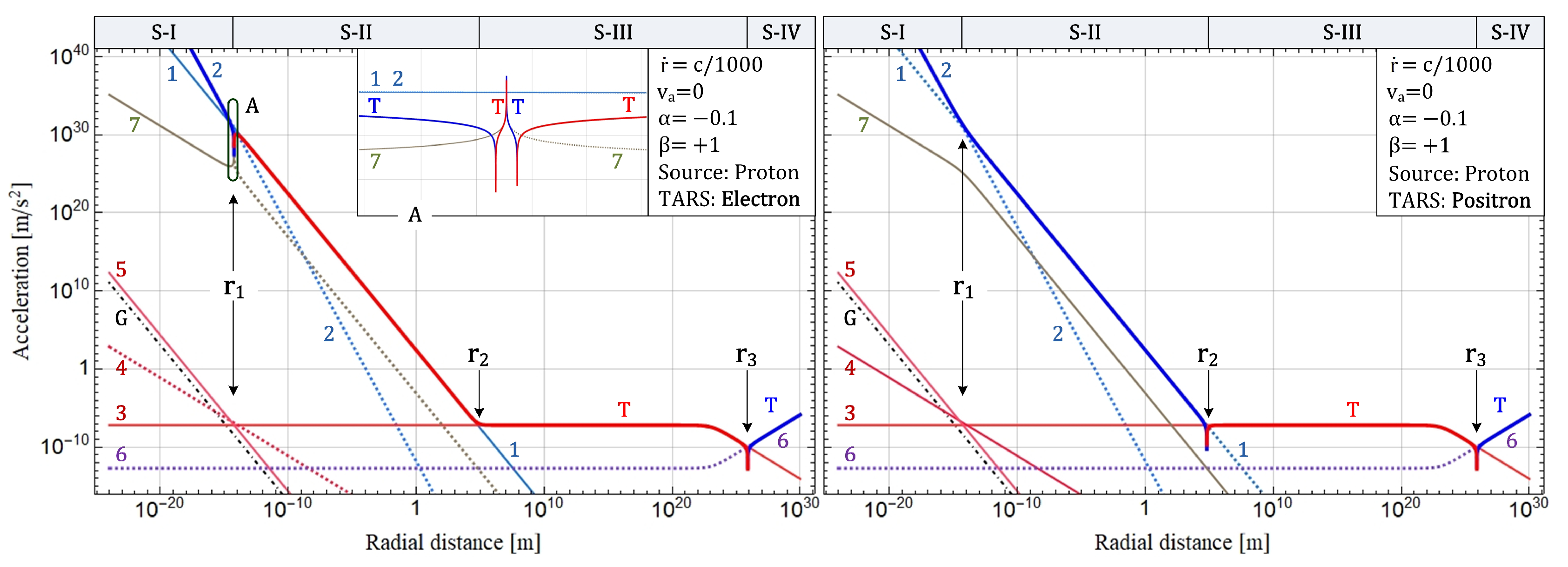
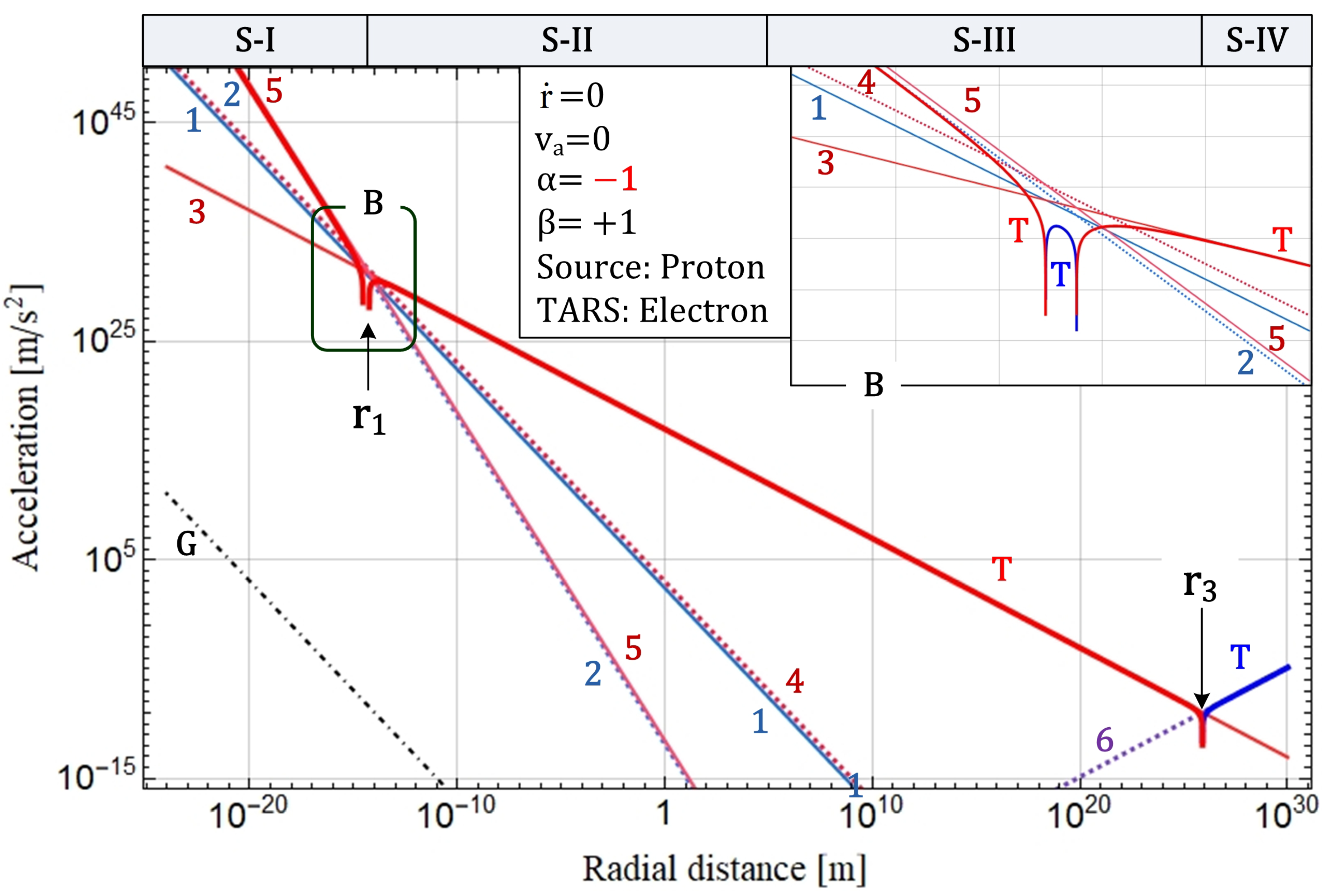
Now, let us consider Figure 1 and Figure 2, obtained by plotting Eq. (25). The physical constants and parameters used in the plotting are as follows:

c = 3.0 \times 10^{8} m / s

k_{e} = 8.987 \times 10^{9} N m^{2} C^{- 2}

e = 1.602 \times 10^{- 19} C

H_{0} = 2.2 \times 10^{- 18} s^{- 1}

χ = 1.759 \times 10^{11} C / k g

α = - 0.1

β = 1

\dot{r} = c / 1000

(in Figure 1) and

0 m / s

(in Figure 2), and

v_{a} = 0

. Mathematica codes, which were used for this plotting, can be found in Appendix E and Appendix F.

From Figure 1 and Figure 2, we can find some interesting aspects, as follows:

[A1]: Based on three intersection points at $r_{1} \sim 5.6 \times 10^{- 15} m$ , $r_{2} \sim 1.4 \times 10^{3} m$ , and $r_{3} \sim 7.6 \times 10^{25} m$ , the whole space can be divided into four distinct shells S-I to S-IV, which are governed by different terms $a_{2}, a_{1}, a_{3}$ , and $a_{6}$ , respectively.
[A2]: The total acceleration in the shell S-IV is positive, as discussed in Sec. 3.1. Meanwhile, using the mathematica codes, one can find that, in order to obtain such a positive acceleration and the distance of 8.1 billion ly (calculated in Sec. 3.1) as the value of $r_{3}$ , the parameter $β$ should be a value close to +1, as assumed for the plotting. Thus, hereinafter, we will refer to the value of $β$ as $+ 1$ . In addition, since, except for the value of $r_{3}$ , most of the results discussed in this article are less sensitive to the value of $β$ , we will suppose that this choice is valid. This means that we will use the Hubble’s law as it is.
[A3]: The total acceleration in the shell S-III has an almost constant negative value. According to Newtonian physics, this gives the result of $v_{s t a r} \sim \sqrt{r}$ , which may allow us to explain the galaxy rotation anomaly[18], without invoking the dark matter hypothesis[19]. Meanwhile, the above-stated boosting effect will make the gradient of the distribution factor steeper, and thus, this effect may also be partly responsible for the galaxy rotation anomaly.
[A4]: At $r = 10^{- 16} m$ , a ratio between strengths of the curves 2, 1, 7, and 5 is about $1 : 10^{- 2} : 10^{- 8} : 10^{- 38}$ that is similar to that between the known four fundamental forces. Based on this clue, hereinafter, we will examine whether $a_{2}, a_{1}, a_{7}$ , and $a_{5}$ can be interpreted as the strong, electric, weak, and gravitational terms.
[A5]: In particular, the term $a_{5}$ obeys the law of inverse square and has a direction independent of the sign of electric charge, because it is written in the form of ${\tilde{k}}^{2} / r^{2}$ . Especially, it should be noted that, despite the fact that the Newton constant is not used to plot the curve 5, the curve 5 is plotted along and very close to a reference line G showing the gravitational field of the proton, as shown in Figure 1. In this sense, we can strongly suspect that the term $a_{5}$ is responsible for the gravitational force.

However, we can also find some perplexing aspects, as follows:

[B1]: In the shell S-III, the term $a_{3}$ is excessively high, compared with the reasonable value (e.g., of about $10^{- 10} m / s$ in the MOND theory[20]). Similarly, there is a slight discrepancy in strength between the curves 5 and G.
[B2]: The point $r_{1}$ is slightly different from the known proton radius $0.8 \times 10^{- 15} m$ .
[B3]: There is an issue in direction of each of the terms $a_{2}$ , $a_{3}$ , and $a_{5}$ . In detail, the term $a_{2}$ is always repulsive, and thus, it is clear that the strong force cannot be explained by the term $a_{2}$ alone. Also, the terms $a_{3}$ and $a_{5}$ are attractive or repulsive, depending on a sign of $α W_{r}$ , although they are independent of the sign of electric charge. This means that there are difficulties in explaining the galaxy rotation anomaly and the gravitational force through the terms $a_{3}$ and $a_{5}$ .
[B4]: At the moment, it is unclear that the term $a_{7}$ is responsible for the weak force.

3.10. Some Possibilities for Perplexing Aspects

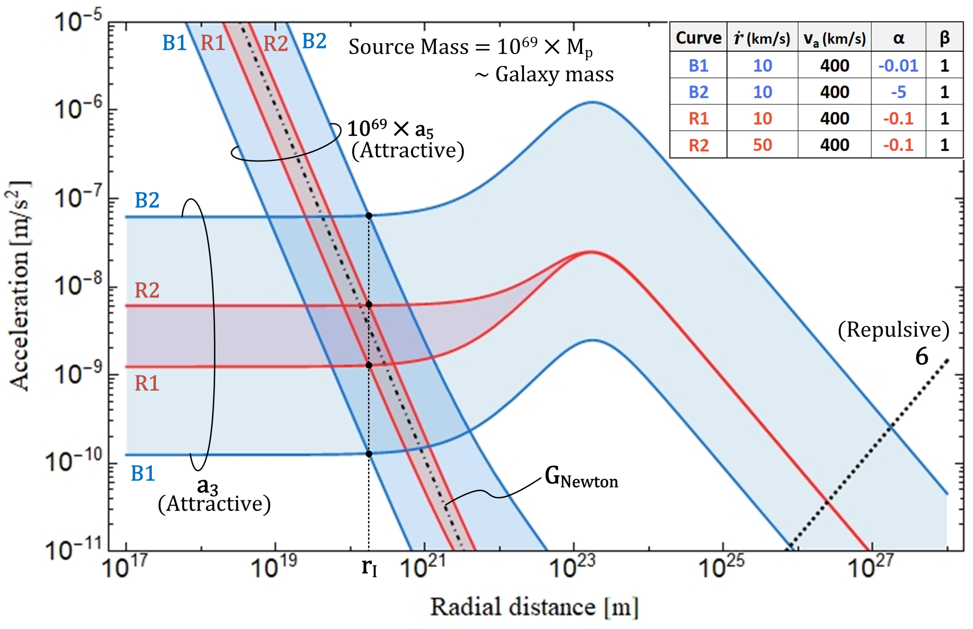
With regard to the issue [B1], the mentioned differences can be reduced or eliminated by adjusting the values of

α

and

\dot{r}

, as exemplarily shown in Figure 3. If so, why should they be such values? Our ideas on this topic will be mentioned in the following discussion on the issue [B3].

With regard to the issue [B2], we have not considered the substructure (i.e., quarks) of the proton. This means that there is a chance of solving this issue and that further research is needed.

With regard to the issue [B3], although, as stated above, the always-repulsive second term

a_{2}

alone cannot explain the strong force, this problem can be alleviated, if the repulsive term

a_{2}

is overwhelmed by any other attractive term. Fortunately, there seems to be such a term. For example, the repulsive term

a_{2}

is overwhelmed by the attractive term

a_{5}

, if

α < - 1 / 2

for

\dot{r} = v_{a} = 0

(see Figure 2) or

α < 0

for

\dot{r} = - H_{0} r

and

v_{a} = 0

. This overwhelming condition can be satisfied for a short time period (although not always), if the neglected velocities

v_{T}

v_{O}

, and

v_{R}

are considered, but if

- α

is sufficiently large in the shell S-I, the term

a_{5}

can suppress the term

a_{2}

in a time-averaged manner. For this reason, we conjecture that the strong force or the asymptotic freedom in the shell S-I would be related to a time-averaged behavior of the combined terms

a_{5}

and

a_{2}

Meanwhile, in order to explain the galaxy rotation anomaly in the shell S-III, the parameter

α

is expected to be a small value (e.g., of about

- 0.01

) (see Figure 3). This means that the parameter

α

has different values in the shells S-I and S-III; that is, in order to explain both of the strong force in S-I and the galaxy rotation anomaly in S-III, the parameter

α

should depend on distance. In this regard, it would be worth noting the facts that a difference in

Λ

-value between the primordial and present epochs is similar to that between the shells S-I and S-III and that there is a difference in

Λ^{- 1} \partial_{t} Λ

α

between the primordial and present epochs (see Eq. (15)). Based on these similarities, we conjecture that there will be a difference in

Λ^{- 1} \partial_{t} Λ

α

between the shells S-I and S-III. This means that the dependence of

α

on distance could be true, but it is also true that further research is needed.

Next, in order to make the terms

a_{3}

and

a_{5}

attractive,

α / (\dot{r} + H_{0} r)

(for

v_{a} = 0

) or

α W_{r}

(for general cases) should be negative (see Eqs. (25) and (26)) 3. This means that the parameter

α

should have dependence on the velocity of TARS or time. In this regard, it should be noted that the LHS of Eq. (23) is generally neither zero nor constant. This shows that the parameter

α

can be changed with time. Thus, if we found a solution for

α

from Eq. (7) or (23), we could further examine whether there is a story capable of explaining the gravitational and strong forces. As of now, we can just conjecture that the Hubble expansion and the quantum phenomena, which affect the LHS of Eq. (23), are closely related to the gravitational and strong forces.

With regard to the directions of the terms

a_{3}

and

a_{5}

, there is another possibility, even when the parameter

α

has a fixed sign. Due to the Hubble expansion effect, the

W_{r}

factor of Eq. (26) is symmetric about a line of

\dot{r} = - H_{0} r

, which is offset from an intuitively natural line of

\dot{r} = 0

. In the

W_{r}

-containing terms

a_{3}

a_{5}

, symmetric effects about the line of

\dot{r} = 0

will be canceled, and only asymmetric effects will be left as a non-vanishing acceleration. Due to such a remnant asymmetric acceleration effect by the

W_{r}

factor, the term

a_{5}

would have a fixed direction in a time-averaged behavior, although not in an instantaneous behavior, if the parameter

α

has a fixed sign. However, if this scenario is true, it means that we have to abandon our belief that a gravitational force exerted on a single elementary particle has a fixed direction always; in other words, the direction of the gravitational force may be a time-averaged property of a collective object, which is composed of a number of particles. Of course, in order to know whether this scenario is true, it is necessary to formulate the time-averaged or collective behavior of the remnant asymmetric effect in the

W_{r}

-containing terms

a_{3}

a_{5}

. Although I have failed to formulate this, this scenario seems plausible, at least until now, in that there has been no gravity experiment for a single particle[22]. In addition, this scenario may be somewhat related to the emergent gravity theories[23,24].

Meanwhile, there is an elusive, but, interesting aspect on the infinite acceleration at

\dot{r} = - H_{0} r

. For example, it seems to require a step of kicking an object with the infinite acceleration, in a velocity-changing process. This means that the velocity is changed in a stepwise manner. Presumably, the kicking step of the infinite acceleration may be an underlying cause of the wave nature of matter, which is the most fundamental difficulty in understanding the quantum phenomena, and/or of the bosenova phenomenon[25].

With regard to the issue [B4], due to its

S_{p} {(r)}^{2}

(i.e.,

Λ_{-} {(r)}^{2}

) factor, the term

a_{7}

is stronger than any other terms near the point

r_{1}

and is attractive and repulsive inside and outside the point

r_{1}

, as shown in the small box of Figure 1. Here, due to the fact that the term

a_{7}

has opposite directions inside and outside the point

r_{1}

, we can say that the term

a_{7}

serves as an outward pulling force on the point

r_{1}

and leads to a reduction in stability of the object, under a certain condition. Also, due to the fact that the term

a_{7}

is stronger than any other terms near the point

r_{1}

, we can say that the term

a_{7}

possesses the ability to cause a decay of the object, beyond the reduction in stability, under a certain condition. In this sense, we conjecture that if we take the chirality of a particle, as the mentioned condition, into consideration, we might find something related to the beta decay or the weak interaction.

4. Proposal of Experimental Tests

Now, we propose experimental tests to verify our approach. First, according to our results, in the shell S-III beyond

r_{2}

, the electric field (i.e.,

a_{1}

) is overwhelmed by the term

a_{3}

mentioned to explain the galaxy rotation curve (see Figure 1). Although it depends on the parameters, the presence of such an inflection point

r_{2}

has not been expected in most of the fundamental theories, except for the MOND theory, and thus, our approach can be decisively tested by examining whether

r_{2}

is present or not. Second, the terms

a_{3}

a_{5}

give very large accelerations at a very small velocity (i.e., low temperature), because of the

W_{r}

factor. Especially, such accelerations would be changed abruptly from

+ \infty

- \infty

or vice versa, at a special velocity of

\dot{r} = - H_{0} r

and

v_{a} = 0

or at a corresponding temperature, if the parameter

α

has a fixed sign. This large acceleration or its abrupt change could be easily measured. Perhaps, this process may be related to the Bosenova phenomenon[25], mentioned above.

5. Conclusions

Until now, we have tried to convince the reader that our approach based on the proportional equation and the multiplicative superposition can provide new clues to some fundamental problems. For example, by considering the temporal variation of the distribution factor, we have shown that there are meaningful clues to the cosmological problems, such as the inflationary and accelerating expansions of the universe and the missing mass problem, and that the electric force can be split into eight distinct forces. However, it is true that there are still some unclear aspects in our approach on gravity and quantum physics. Thus, in order to know whether they are true clues, it is necessary to conduct further research in the context of the existing physics, such as thermodynamics and field theories, in addition to the proposed experimental tests. We think that understanding Eq. (7) or (23) would be important in this process.

Acknowledgments

I am sincerely grateful to Lee, J.P. for his lecture, allowing me to escape a problem that I had been trapped for 20 years.

Appendix A. Comments on Postulate 2

Roughly speaking, our approach (hereinafter, OA) will be developed in a similar way to the general relativity (GR), except for a difference in interpretation of nature of matter and space (i.e., in the space model) and a difference in formulation method originated from that. Because of such differences in space model and formulation method, there is also a difference in starting points (i.e., postulates) between GR and OA. Although a postulate is a statement that is taken to be true, if it is written in a form different from that in a successful known theory, it may be difficult to agree to the postulate immediately. Thus, in order to reduce misunderstanding associated with the difference between postulates, here we will briefly review the similarities and differences between GR and OA and then explain why such differences are necessary.

•: Summary of GR and OA

In GR, from the following equation (A1) representing the equivalence principle, we obtain an equation of motion (A2), which can describe a trajectory of an object to be observed by an observer in the laboratory. This process is substantially a coordinate transformation process, in which the chain rule is used, and the Christoffel symbols of Eq. (A2) are calculated using a metric tensor. In a sense, the use of chain rule and metric tensor can be understood as a process of projecting Eq. (A1) or (A2) onto a reference frame of the laboratory observer.

\begin{matrix} \frac{d^{2} ξ^{α}}{d τ^{2}} & = 0, and \end{matrix}

(A1)

\begin{matrix} \frac{d^{2} x^{λ}}{d t^{2}} & = - Γ_{μ ν}^{λ} + \frac{d x^{μ}}{d t} \frac{x^{ν}}{d t} + Γ_{μ ν}^{0} \frac{d x^{μ}}{d t} \frac{d x^{ν}}{d t} \frac{d x^{λ}}{d t} . \end{matrix}

(A2)

In OA, from the following equation (A3) given as a postulate, we obtain an equation of motion (A4) valid for Cooper. Next, we obtain an equation of motion (A5) valid for Murphy or the laboratory observer, from Eq. (A4). Here, the derivation of Eq. (A5) is a coordinate transformation process, in which the chain rule is used, and the Christoffel symbols and

V^{2}

in Eq. (A5) are calculated using a metric tensor. (See Appendix C and Appendix D.) As in the case of GR, the use of chain rule and metric tensor can be understood as a process of projecting Cooper’s description onto Murphy’s frame.

\begin{matrix} ε (X^{i}, V, p) & = ψ_{0} \frac{γ (V)}{Λ (X^{i}, p)} = constant, \end{matrix}

(A3)

\begin{matrix} A & = \frac{c^{2}}{μ γ^{2}} [\frac{\partial μ}{\partial p} \frac{V}{V^{2}} + \tilde{\nabla} μ], and \end{matrix}

(A4)

\frac{d^{2} x^{k}}{d t^{2}} = \frac{c^{2}}{γ^{2}} [(\frac{1}{μ} \frac{\partial μ}{\partial t}) \frac{v^{k}}{V^{2}} + \frac{1}{h_{0}^{2} h_{k}^{2}} (\frac{1}{μ} \frac{\partial μ}{\partial x^{k}})] - \frac{d x^{k}}{d t} (\frac{1}{h_{0}} \frac{d h_{0}}{d t}) - Γ_{j β}^{k} \frac{d x^{j}}{d t} \frac{d x^{β}}{d t},

(A5)

•: Similarities and differences between GR and OA

There are at least two common points between GR and OA.

(C1): Starting equations (A1) and (A3) are supposed to be valid for a specific observer (i.e., for a free falling observer in GR and for Cooper in OA) in only a small or local region in the spacetime.
(C2): A metric tensor is used to project the starting equation onto a reference frame of the laboratory observer (i.e., Murphy).

There are at least three different points between GR and OA.

(D1): There is a difference in form between the starting equations (A1) and (A3)).
(D2): There is a difference in physical state between chosen observers, for whom the starting equations are valid.
(D3): There is a difference in physical meanings of the metric tensor. This topic will be explained in Appendix B.

•: Difference in physical state between observers and its implications

Now, we will explain differences in physical state between three observers, which will be mentioned in OA or GR. Here, the free falling observer in GR corresponds to TARS in OA, so hereinafter he or she will be referred to as TARS.

The physical state of each observer can be definitely specified by position, velocity, and acceleration. In this article, Murphy is supposed as an observer at rest in the laboratory, for convenience, although, in general, she can be in an arbitrary state. Thus, there may be differences in all of position, velocity, and acceleration between TARS and Murphy. By contrast, according to the definition given for Cooper, there may be a difference in only velocity between Cooper and TARS, and there may be differences in only position and acceleration between Cooper and Murphy. That is, by introducing Cooper, we can decompose the differences in observers physical state into two parts: a difference in position and differences in velocity and acceleration.

Here, it should be noted that only the difference in velocity is allowed between Cooper and TARS. Considering this difference in velocity allowed between Cooper and TARS, it is natural that there is a difference in form between the starting equations for Cooper and TARS, mentioned above. The starting equation (A1) in GR states that the velocity of the target object measured by TARS is zero (i.e., constant), but Cooper can no longer say the constancy in velocity of the target object, because a velocity measured by Cooper can be constantly changed. That is, the starting equation (A1) in GR is no longer valid for Cooper.

•: Constant of motion

Meanwhile, finding a constant of motion, such as the constancy in velocity given by Eq. (A1), is very useful in physics, and this is true for Cooper’s description. As noted above, the velocity (i.e., state of motion) of the target object observed by Cooper is not fixed. If such a change in velocity is unavoidable in Cooper’s description, it is necessary to find the constant of motion for Cooper elsewhere. We will find it from the causality principle, which states that a change in cause produces a change in effect. From a causal point of view, we can say that a change in velocity is closely related to a change in effect produced by a change in cause. This means that Cooper has a chance to find the constant of motion from a certain combination of the changes in cause and effect.

If so, next issues are to determine how to express each of the changes in cause and effect and how to combine them. Probably, these issues will correspond to metaphysical questions, which cannot be answered within physics. Thus, as stated by Eq. (A3), we will postulate that 1) the changes in cause and effect can be properly described using the Lorentz and distribution factors, respectively and 2) we can have a truly correct answer if and only if a ratio, not a sum, is selected as a mathematical method of combining the Lorentz and distribution factors and the ratio is supposed to be constant.

It is worth noting that, in GR, a change in cause is given based on an additional constraint (i.e., the Einstein field equation) not by the starting equation itself (i.e., the geodesic equation), while, in OA, the starting equation (i.e., Eq. (A3)) is represented through the combination of changes in cause and effect.

One might find that, except for the differences in physical quantities representing the cause and effect and in the mathematical method of combining them, the expression of Eq. (A3) is closely related to the energy conservation law in classical physics. This finding is true, and we will find in Sec. 3.3 that Eq. (A3) is another expression of the energy conservation law.

Appendix B. Comments on Postulate 3

Here, we explain a basic method of constructing a metric tensor, based on the inherent quantitative properties of the Mach fluid. This is intended to show that the metric tensor can have an alternative physical meaning, under our 1-based space model. However, this method is not mature enough to allow for comprehensive discussions on general systems or three systems to be discussed in this article, and it is necessary to generalize this method through a more rigorous mathematical approach. Due to this limitation, we have no choice but to introduce Eqs. (4)-(6) as the postulate 3, and we hope that, from the following explanation, the reader can find that the postulate 3 is reasonable or is close to true, and moreover, that someone can find a more general theory.

The reader will find that a term "the same Mach quantity" is used as a keyword in our discussion below. This is because our discussion is based on an underlying principle (hereinafter, same-phenomenon-same-quantity (SPSQ) principle), which states that the Mach quantity involved in the same physical phenomenon is the same. It can be said that the method described here is part of the process of formulating the SPSQ principle.

The Mach density

ρ

mentioned in the main text can be defined as a quantity of Mach fluid that is contained in a three-dimensional box with a given volume (i.e.,

ρ = Q / V

). By fixing one of Q and V and examining a change of the other, we can describe a change in Mach density. In this article, the change of Mach density will be described in a manner of fixing the Mach quantity to

Q_{0}

and examining a spatial and temporal variation of the volume. That is,

ρ (r, t) = Q_{0} / V (r, t)

•: Ratios between spatial lengths: Eq. (4) in the main text

First, let us choose a rectangular box as the three-dimensional box, which will be used to define the volume

V (r, t)

. Then, the rectangular box’s volume

V (r, t)

at an arbitrary point

(r, t)

in spacetime is given as the product of lengths,

{\hat{e}}_{i}

, of three orthogonal sides of the rectangular box: i.e.,

V (r, t) = \prod_{i = 1}^{3} {\hat{e}}_{i} (r, t)

, where

i = 1, 2, 3

. Next, suppose that two rectangular boxes are respectively located at reference and arbitrary points (

r_{0}, t_{0}

) and (

r, t

) in spacetime. Then, due to the requirement of the same Mach quantity, the boxes may have different volumes. In this case, ratios between the side lengths of the boxes can be described by scale factors

s_{i} (r, t)

, as follows.

{\hat{e}}_{i} (r, t) = s_{i} (r, t) {\hat{e}}_{i} (r_{0}, t_{0}) .

(A6)

Here, due to the requirement of the same Mach quantity, we can impose the following constraint on the scale factors

s_{i} (r, t)

ρ (r, t) = ρ_{0} / \prod_{i = 1}^{3} s_{i} (r, t)

, where

ρ_{0} = Q_{0} / \prod_{i = 1}^{3} {\hat{e}}_{i} (r_{0}, t_{0})

Next, the three orthogonal sides of each box can be used as three spatial basis vectors for an orthogonal reference frame, at a region where the box is located. For convenience, let us introduce a new factor (hereinafter, a distribution factor) of

Λ_{i} (r, t) = 1 / s_{i} (r, t)

. Then, we can write the relationship between lengths of the corresponding basis vectors in the two reference frames, as follows:

{\hat{X}}_{i} = \frac{1}{Λ_{i} (r, t)} {\hat{x}}_{i},

(A7)

where

{\hat{X}}_{i} = {\hat{e}}_{i} (r, t)

and

{\hat{x}}_{i} = {\hat{e}}_{i} (r_{0}, t_{0})

. Here, due to the above constraint on

s_{i} (r, t)

Λ_{i} (r, t)

should be constrained by the following formula.

\prod_{i = 1}^{3} Λ_{i} (r, t) = ρ (r, t) / ρ_{0} .

(A8)

A change in length of a basis vector leads to a change in distance between two points arranged parallel to the basis vector (i.e., in coordinate length). In detail, a change in coordinate length is inversely proportional to a change in length of the basis vector. Meanwhile, if

Λ_{i} (r, t)

is spatially or temporally changed, the relation given by Eq. (A7) will be valid only in a small region or a short time interval. Therefore, ratios between the coordinate lengths at

(r_{0}, t_{0})

and

(r, t)

should be written in an infinitesimal manner, as follows:

d X^{i} = Λ_{i} (r, t) d x^{i} .

(A9)

•: Ratios between temporal lengths: Eq. (5) in the main text

Similar to the above, the requirement of the same Mach quantity can also be used to define relationships between temporal lengths and Mach densities. A spatial volume, which is swept by a light beam during a given time interval (

Δ t_{0}^{'}

Δ t_{0}

), can be given by the product of a sectional area (

A_{0}^{'}

A_{0}

) of the beam and a traveling distance (

c^{'} Δ t_{0}^{'}

c Δ t_{0}

). Thus, the requirement of the same Mach quantity at regions of

ρ (r, t)

and

ρ_{0}

can be formulated by the following equation.

ρ (r, t) c^{'} Δ t_{0}^{'} A_{0}^{'} = ρ_{0} c Δ t_{0} A_{0} .

(A10)

Next, using the above equation (A8), Eq. (A10) can be rewritten as follows:

c^{'} Δ t_{0}^{'} A_{0}^{'} = c Δ t_{0} A_{0} / \prod_{i = 1}^{3} Λ_{i} (r, t) .

(A11)

The sectional area of the beam is determined by the shape of a light source, which is independent of the propagation of light (i.e., irrelevant to a time-involved physical phenomenon). Excluding the contribution by such a phenomenon-independent sectional area, Eq. (A11) can be rewritten as follows.

c^{'} d t^{'} = \frac{1}{Λ (r, t)} c d t .

(A12)

•: At least one postulate is needed

In a sense, Eq. (A9) can be obtained directly from the definition of Mach density. Although this process includes a step of constructing a coordinate system using a rectangular box, the using of the box is independent of a time-involved phenomenon and thus does not require any a priori postulate. By contrast, in order to go from Eq. (A12) to Eq. (5) of the main text, we should introduce a priori postulate related to phenomena. It is clear that the postulate should be the constancy of light speed (i.e.,

c^{'} = c

). In other words, we can obtain Eqs. (A9) and (A12) on the basis of the 1-based model, but at least one a priori postulate should be introduced to change Eq. (A12) to Eq. (5). Owing to this necessity of postulate, Eqs. (4) and (5) are introduced as part of the postulate 3.4

•: Metric tensor for spherically symmetric system

For a static spherically symmetric system, it is known that due to its spherical symmetry, a metric tensor can be given, as follows:

d s^{2} = B (r) c^{2} d t^{2} - A (r) d r^{2} - r^{2} d θ^{2} - r^{2} s i n^{2} θ d ϕ^{2} .

(A13)

In the general theory of relativity, using the Einsteins field equation (EFE) and the weak field approximation, we can show that

\begin{matrix} A (r) & B (r) = 1, and \end{matrix}

(A14)

\begin{matrix} A (r) & = {(1 - \frac{2 G M}{r c^{2}})}^{- 1} . \end{matrix}

(A15)

Meanwhile, it is unclear whether the EFE as it is can be used in our approach, because the EFE is based on the 0-based space model that is different from that in our approach. For example, the matter and space in the EFE are conceptually different from those in our approach, and time dependence mentioned in the EFE is not directly related to dependence of the distribution factor on time in our approach. Nevertheless, we can say that, if we found a generalized method of constructing a metric tensor based on the SPSQ principle, the consequent metric tensor for at least a static spherically symmetric system would have the same form as that in the general relativity. Similarly, even for time-dependent systems, it seems reasonable to conjecture that a metric tensor can be written, as follows:

d s^{2} = \frac{1}{Λ {(r, t)}^{2}} c^{2} d t^{2} - Λ {(r, t)}^{2} d r^{2} - r^{2} d θ^{2} - r^{2}, \sin^{2} θ d ϕ^{2} .

(A16)

Concretely, to justify this conjecture or to go from Eq. (A13) to Eq. (A16), we should do:

1): show $A (r) B (r) = 1$ and $A (r) = Λ {(r)}^{2}$ ,
2): find a method of incorporating the time-dependent distribution factor into the metric, and
3): show that, in a spherical coordinate system, only time and radial components depend on the distribution factor.

Although, as described above, further study is needed to do these, it seems that the steps 1) and 2) could be justified by the above arguments provided for Eqs. (A9) and (A12) and the step 3) could be justified by the spherical symmetry of the system. Thus, in this article, we will assume that Eq. (A16) gives the correct result, as stated by the postulate 3.

Appendix C. Derivation of Eq. (9)

The equation (8) in the main text can be written as follows:

\frac{d V^{i}}{d p} = \frac{c^{2}}{μ γ^{2}} [\frac{\partial μ}{\partial p} (\frac{V^{i}}{{| V |}^{2}}) + \frac{\partial μ}{\partial X^{i}}],

(A17)

where

V^{i} = d X^{i} / d p

and

{| V |}^{2} = V \cdot V

. First, let us calculate two quantities, which will be used in calculation of

d V^{i} / d p

, in advance. Since

X^{i}

is a three-dimensional quantity that does not explicitly have a time coordinate, we can find that

\partial X^{i} / \partial x^{0} = 0

and thus,

V^{i} = \frac{d X^{i}}{d p} = \sum_{α = 0}^{3} \frac{d x^{α}}{d p} \frac{\partial X^{i}}{\partial x^{α}} \to \sum_{j = 1}^{3} \frac{d x^{j}}{d p} \frac{\partial X^{i}}{\partial x^{j}} .

(A18)

Next, according to Eqs. (4) to (6), the quantity

\partial X^{i} / \partial x^{j}

is given by a calibration or distribution factor that is generally dependent on both of position and time. This means that the quantity

\frac{d}{d p} (\frac{\partial X^{i}}{\partial x^{j}})

may not be zero in general, and it can be written as follows:

\frac{d}{d p} (\frac{\partial X^{i}}{\partial x^{j}}) = \sum_{β = 0}^{3} \frac{d x^{β}}{d p} \frac{\partial^{2} X^{i}}{\partial x^{j} \partial x^{β}} .

(A19)

Using these results, the left-hand side of Eq. (A17) can be rewritten as follows:

\frac{d V^{i}}{d p} = \sum_{j} \frac{d^{2} x^{j}}{d p^{2}} \frac{\partial X^{i}}{\partial x^{j}} + \sum_{j, β} \frac{d x^{j}}{d p} \frac{d x^{β}}{d p} \frac{\partial^{2} X^{i}}{\partial x^{j} \partial x^{β}} .

(A20)

Putting Eq. (A20) into Eq. (A17), we find:

\sum_{j} \frac{d^{2} x^{j}}{d p^{2}} \frac{\partial X^{i}}{\partial x^{j}} = \frac{c^{2}}{μ γ^{2}} [\frac{\partial μ}{\partial p} \frac{V^{i}}{{| V |}^{2}} + \frac{\partial μ}{\partial X^{i}}] - \sum_{j, β} \frac{d x^{j}}{d p} \frac{d x^{β}}{d p} \frac{\partial^{2} X^{i}}{\partial x^{j} \partial x^{β}} .

(A21)

Next, multiplying the both sides of Eq. (A21) by

\sum_{i = 1}^{3} \frac{\partial x^{k}}{\partial X^{i}}

, we find

\sum_{i, j} \frac{d^{2} x^{j}}{d p^{2}} \frac{\partial X^{i}}{\partial x^{j}} \frac{\partial x^{k}}{\partial X^{i}} = \sum_{i} \frac{c^{2}}{μ γ^{2}} [\frac{\partial μ}{\partial p} \frac{V^{i}}{{| V |}^{2}} + \frac{\partial μ}{\partial X^{i}}] \frac{\partial x^{k}}{\partial X^{i}} - \sum_{i, j, β} \frac{d x^{j}}{d p} \frac{d x^{β}}{d p} \frac{\partial^{2} X^{i}}{\partial x^{j} \partial x^{β}} \frac{\partial x^{k}}{\partial X^{i}} .

(A22)

This can be written in a simplified form, as follows:

\frac{d^{2} x^{k}}{d p^{2}} = \sum_{i} M^{i} \frac{\partial x^{k}}{\partial X^{i}} - \sum_{j, β} Γ_{j β}^{k} \frac{d x^{j}}{d p} \frac{d x^{β}}{d p},

(A23)

where

M^{i} = \frac{c^{2}}{μ γ^{2}} [\frac{\partial μ}{\partial p} \frac{V^{i}}{{| V |}^{2}} + \frac{\partial μ}{\partial X^{i}}], and

(A24)

Γ_{j β}^{k} = \sum_{i} \frac{\partial^{2} X^{i}}{\partial x^{j} \partial x^{β}} \frac{\partial x^{k}}{\partial X^{i}} .

(A25)

The LHS of Eq. (A23) can be written as follows:

\frac{d^{2} x^{k}}{d p^{2}} = \frac{d t}{d p} \frac{d}{d t} (\frac{d t}{d p} \frac{d x^{k}}{d t}) = \frac{d t}{d p} (\frac{d}{d t} \frac{d t}{d p}) \frac{d x^{k}}{d t} + {(\frac{d t}{d p})}^{2} \frac{d^{2} x^{k}}{d t^{2}} = \frac{d^{2} t}{d p^{2}} \frac{d x^{k}}{d t} + {(\frac{d t}{d p})}^{2} \frac{d^{2} x^{k}}{d t^{2}} .

Using this, Eq. (A23) can be written, as follows:

\frac{d^{2} x^{k}}{d t^{2}} {(\frac{d t}{d p})}^{2} + \frac{d x^{k}}{d t} \frac{d^{2} t}{d p^{2}} = \sum_{i} M^{i} \frac{\partial x^{k}}{\partial X^{i}} - \sum_{j, β} Γ_{j β}^{k} \frac{d x^{j}}{d p} \frac{d x^{β}}{d p} .

(A26)

Next, multiplying the both sides of Eq. (A26) by

{(\frac{d p}{d t})}^{2}

gives

\begin{matrix} \frac{d^{2} x^{k}}{d t^{2}} & = \sum_{i} M^{i} \frac{\partial x^{k}}{\partial X^{i}} {(\frac{d p}{d t})}^{2} - \frac{d x^{k}}{d t} \frac{d^{2} t}{d p^{2}} {(\frac{d p}{d t})}^{2} - \sum_{j, β} Γ_{j β}^{k} \frac{d x^{j}}{d t} \frac{d x^{β}}{d t} . \end{matrix}

(A27)

Now we will change Cooper’s quantities

d X^{i}

and

d p

to Murphy’s ones

d x^{i}

and

d t

, using Eqs. (4) to (6). Hereinafter, we will use the Einstein summation rule, but the calibration factors are not excluded from the summation, because they are not vectors. By using Eqs. (4) and (5), we can find

\frac{\partial x^{k}}{\partial X^{i}} = \frac{1}{h_{k}} δ_{k i}, {(\frac{d p}{d t})}^{2} = \frac{1}{h_{0}^{2}}, and \frac{d^{2} t}{d p^{2}} {(\frac{d p}{d t})}^{2} = \frac{1}{h_{0}} \frac{d h_{0}}{d t},

where

δ_{k i}

is Kronecker delta. Using these, Eq. (A27) can be written, as follows:

\frac{d^{2} x^{k}}{d t^{2}} = M^{k} \frac{1}{h_{k}} \frac{1}{h_{0}^{2}} - \frac{d x^{k}}{d t} (\frac{1}{h_{0}} \frac{d h_{0}}{d t}) - Γ_{j β}^{k} \frac{d x^{j}}{d t} \frac{d x^{β}}{d t} .

(A28)

Using

V^{k} = h_{0} h_{k} \frac{d x^{k}}{d t} = h_{0} h_{k} v^{k}

, we can rewrite

M^{k}

, as follows:

M^{k} = \frac{c^{2}}{μ γ^{2}} [h_{0}^{2} h_{k} \frac{\partial μ}{\partial t} (\frac{v^{k}}{{| V |}^{2}}) + \frac{1}{h_{k}} \frac{\partial μ}{\partial x^{k}}] .

(A29)

Putting Eq. (A29) into Eq. (A28) gives

\frac{d^{2} x^{k}}{d t^{2}} = \frac{c^{2}}{μ γ^{2}} [\frac{\partial μ}{\partial t} \frac{v^{k}}{{| V |}^{2}} + \frac{1}{h_{0}^{2} h_{k}^{2}} \frac{\partial μ}{\partial x^{k}}] - \frac{d x^{k}}{d t} (\frac{1}{h_{0}} \frac{d h_{0}}{d t}) - Γ_{j β}^{k} \frac{d x^{j}}{d t} \frac{d x^{β}}{d t} .

(A30)

Placing the factor

1 / μ

into the square brackets gives

\frac{d^{2} x^{k}}{d t^{2}} = \frac{c^{2}}{γ^{2}} [(\frac{1}{μ} \frac{\partial μ}{\partial t}) \frac{v^{k}}{{| V |}^{2}} + \frac{1}{h_{0}^{2} h_{k}^{2}} (\frac{1}{μ} \frac{\partial μ}{\partial x^{k}})] - \frac{d x^{k}}{d t} (\frac{1}{h_{0}} \frac{d h_{0}}{d t}) - Γ_{j β}^{k} \frac{d x^{j}}{d t} \frac{d x^{β}}{d t} .

(A31)

Appendix D. Derivation of Eqs. (10)-(12)

For a system with a spherically symmetric time-varying distribution factor, by the postulate 3, the calibration factors are given as follows:

h_{0} = Λ (r, t), h_{1} = Λ (r, t) h_{2} = r, h_{3} = r \sin θ .

(A32)

Here, the quantity

Λ

in the 0- and 1-components is independent of the angular coordinates, and thus, the factor

(\frac{1}{Λ} \frac{d Λ}{d t})

can be written as follows:

(\frac{1}{Λ} \frac{d Λ}{d t}) = (\frac{1}{Λ} \frac{\partial Λ}{\partial t}) + \sum_{j} (\frac{1}{Λ} \frac{\partial Λ}{\partial x^{j}} \frac{d x^{j}}{d t}) = (\frac{1}{Λ} \frac{\partial Λ}{\partial t}) + (\frac{1}{Λ} \frac{\partial Λ}{\partial r}) \frac{d r}{d t} .

(A33)

Using Eqs. (3) and (A33) and

\frac{1}{μ} \frac{d μ}{d t} = \frac{1}{Λ} \frac{d Λ}{d t}

, we can rewrite Eq. (9) in the main text, as follows:

\begin{matrix} \frac{d^{2} x^{k}}{d t^{2}} & = (\frac{c^{2}}{{| V |}^{2}} - 2) (\frac{1}{Λ} \frac{\partial Λ}{\partial t}) \frac{d x^{k}}{d t} + (\frac{c^{2}}{{| V |}^{2}} - 1) \frac{{| V |}^{2}}{Λ^{2} h_{k}^{2}} (\frac{1}{Λ} \frac{\partial Λ}{\partial x^{k}}) \\ - (\frac{1}{Λ} \frac{\partial Λ}{\partial r}) \frac{d r}{d t} \frac{d x^{k}}{d t} - Γ_{j β}^{k} \frac{d x^{j}}{d t} \frac{d x^{β}}{d t} . \end{matrix}

(A34)

Non-vanishing terms of the Christoffel symbol for this system are as follows:

\{\begin{matrix} Γ_{r t}^{r} = \frac{1}{Λ} \frac{\partial Λ}{\partial t}, Γ_{r r}^{r} = \frac{1}{Λ} \frac{\partial Λ}{\partial r}, Γ_{θ θ}^{r} = - \frac{r}{Λ^{2}}, Γ_{φ φ}^{r} = - \frac{r \sin^{2} θ}{Λ^{2}} \\ Γ_{r θ}^{θ} = \frac{1}{r}, Γ_{φ φ}^{θ} = - \cos θ \sin θ, Γ_{r φ}^{φ} = \frac{1}{r}, Γ_{θ φ}^{φ} = \cot θ . \end{matrix}

(A35)

Using the results of Eq. (A35), we can calculate the last term of Eq. (A34) as follows:

\begin{matrix} \{\begin{matrix} - Γ_{j β}^{r} \frac{d x^{j}}{d t} \frac{d x^{β}}{d t} & = - Γ_{r t}^{r} \dot{r} - Γ_{r r}^{r} {\dot{r}}^{2} - Γ_{θ θ}^{r} {\dot{θ}}^{2} - Γ_{φ φ}^{r} {\dot{φ}}^{2} \\ = - \frac{1}{Λ} \frac{\partial Λ}{\partial t} \dot{r} - \frac{1}{Λ} \frac{\partial Λ}{\partial r} {\dot{r}}^{2} + \frac{r}{Λ^{2}} {\dot{θ}}^{2} + \frac{r \sin^{2} θ}{Λ^{2}} {\dot{φ}}^{2} \\ - Γ_{j β}^{θ} \frac{d x^{j}}{d t} \frac{d x^{β}}{d t} & = - 2 Γ_{r θ}^{θ} \dot{r} \dot{θ} - Γ_{φ φ}^{θ} {\dot{φ}}^{2} \\ = - \frac{2}{r} \dot{r} \dot{θ} + \cos θ \sin θ {\dot{φ}}^{2} \\ - Γ_{j β}^{φ} \frac{d x^{j}}{d t} \frac{d x^{β}}{d t} & = - 2 Γ_{r φ}^{φ} \dot{r} \dot{φ} - 2 Γ_{θ φ}^{φ} \dot{θ} \dot{φ} \\ = - 2 \frac{1}{r} \dot{r} \dot{φ} - 2 \cot θ \dot{θ} \dot{φ} . \end{matrix} \end{matrix}

(A36)

Using the results of Eqs. (A32) and (A36), we can obtain each component of Eq. (A34) as follows:

\begin{matrix} \{\begin{matrix} \frac{d^{2} r}{d t^{2}} = (\frac{c^{2}}{{| V |}^{2}} - 3) (\frac{1}{Λ} \frac{\partial Λ}{\partial t}) \dot{r} + (\frac{c^{2}}{{| V |}^{2}} - 1) \frac{{| V |}^{2}}{Λ^{4}} (\frac{1}{Λ} \frac{\partial Λ}{\partial r}) - \frac{2}{Λ} \frac{\partial Λ}{\partial r} {\dot{r}}^{2} + \frac{r}{Λ^{2}} {\dot{θ}}^{2} + \frac{r \sin^{2} θ}{Λ^{2}} {\dot{φ}}^{2} \\ \frac{d^{2} θ}{d t^{2}} = (\frac{c^{2}}{{| V |}^{2}} - 2) (\frac{1}{Λ} \frac{\partial Λ}{\partial t}) \dot{θ} - \frac{1}{Λ} \frac{\partial Λ}{\partial r} \dot{r} \dot{θ} - \frac{2}{r} \dot{r} \dot{θ} + \cos θ \sin θ {\dot{φ}}^{2} \\ \frac{d^{2} φ}{d t^{2}} = (\frac{c^{2}}{{| V |}^{2}} - 2) (\frac{1}{Λ} \frac{\partial Λ}{\partial t}) \dot{φ} - \frac{1}{Λ} \frac{\partial Λ}{\partial r} \dot{r} \dot{φ} - \frac{2}{r} \dot{r} \dot{φ} - 2 \cot θ \dot{θ} \dot{φ} . \end{matrix} \end{matrix}

(A37)

The third term in RHS of the radial component in Eq. (A37) can be re-written as follows:

- \frac{2}{Λ} \frac{\partial Λ}{\partial r} {\dot{r}}^{2} = - \frac{2}{Λ} \frac{\partial Λ}{\partial r} ({\dot{r}}^{2} + \frac{r^{2} {\dot{θ}}^{2}}{Λ^{2}} + \frac{r^{2} \sin^{2} θ {\dot{φ}}^{2}}{Λ^{2}}) + \frac{2}{Λ} \frac{\partial Λ}{\partial r} (\frac{r^{2} {\dot{θ}}^{2}}{Λ^{2}} + \frac{r^{2} \sin^{2} θ {\dot{φ}}^{2}}{Λ^{2}}) .

(A38)

Meanwhile, using Eq. (A32), we can find

\frac{{| V |}^{2}}{Λ^{4}} = ({\dot{r}}^{2} + \frac{r^{2} {\dot{θ}}^{2}}{Λ^{2}} + \frac{r^{2} \sin^{2} θ {\dot{φ}}^{2}}{Λ^{2}}) .

(A39)

Using Eqs. (A38) and (A39), the radial component of Eq. (A37) can be written as follows:

\frac{d^{2} r}{d t^{2}} = (\frac{c^{2}}{{| V |}^{2}} - 3) [(\frac{1}{Λ} \frac{\partial Λ}{\partial t}) \dot{r} + \frac{{| V |}^{2}}{Λ^{4}} (\frac{1}{Λ} \frac{\partial Λ}{\partial r})] + (\frac{2}{Λ} \frac{\partial Λ}{\partial r} + \frac{1}{r}) \frac{r^{2} {\dot{Ω}}^{2}}{Λ^{2}},

(A40)

where

{\dot{Ω}}^{2} = {\dot{θ}}^{2} + \sin^{2} θ {\dot{φ}}^{2}

Appendix E. Mathematica code for Figure 1 and Figure 2

ClearAll@"`*"

(*Acceleration Terms*)

at1=FullSimplify[k/r^2];

at2=FullSimplify[(2 k^2)/(r^3 c^2)] ;

at3=FullSimplify[(\[Alpha] H \[DoubleStruckCapitalW] c^2)];

at4=FullSimplify[(4 \[Alpha] H \[DoubleStruckCapitalW] k)/r];

at5=FullSimplify[(\[Alpha] H \[DoubleStruckCapitalW] ((2 k)/(r c))^2)] 10^pno;

at6=FullSimplify[-3 \[Alpha] \[Beta] H^2 r -3 \[Alpha] H vr];

at7=FullSimplify[-((3 k ( \[Beta] H r + vr)^2)/((1+(2 k)/(r c^2)) (r^2 c^2)))];

at8a=0*FullSimplify[(k va^2)/ (r^2 c^2)]; (*<<Note 0* *)

at8b= 0*FullSimplify[va^2/r]; (*<<Note 0* *)

Tot=FullSimplify[at1+at2+at3+at4+at5+at6+at7+at8a+at8b];

(* Physical constants *)

c=3*10^8;

CoulmbC=8.987*10^9;

elmchrg=1.602*10^-19;

NewtonC=6.674*10^-11;

ProtonM=1.672*10^-27;

ElectnM=9.109*10^-31;

k=CoulmbC*elmchrg^2 *qs*qt *(ms/ProtonM)*(1/mt);

va= va0 ;

vr=vr0 Cos[th];

\[DoubleStruckCapitalW]= ( \[Beta] H r +vr)/(( \[Beta] H r +vr)^2+va^2 (1+(2 k)/(r c^2)));

(* Plotting of Acceleration terms *)

SetOptions[Manipulator,Appearance->"Close"];

Manipulate[

PRM= {vr0->v1, va0->v2, H->2.2 *10^HP, th->phase, mt->Mt, ms->Ms, pno->no, qt->Qt, qs->Qs,

\[Alpha]->BB1, \[Beta]->BB2};

STYL1={Thickness->0.004,Dashing[0.004]};

STYL2={Thickness->0.003};

LogLogPlot[{Abs[- k /r^2]/.PRM, Abs[-NewtonC ms * 10^pno /r^2]/.PRM,

+at1/.PRM,-at1/.PRM,+at2/.PRM,-at2/.PRM,+at3/.PRM,-at3/.PRM,+at4/.PRM,-at4/.PRM,+at5/.PRM,-at5/.PRM,

+at6/.PRM,-at6/.PRM,+at7/.PRM,-at7/.PRM,+at8a/.PRM,-at8a/.PRM,+at8b/.PRM,-at8b/.PRM,+Tot/.PRM,-Tot/.PRM},

{r,10^LP,10^UP}, PlotRange->{10^s1, 10^s2},

FrameLabel->{Text[Style["Radial distance [m]",22,FontFamily->"Times"]],

Text[Style["Acceleration [m/s^2]",22,FontFamily->"Times"]]},

Frame->True,FrameStyle->Directive[Black,21],LabelStyle->Directive[Black,22],

PerformanceGoal->"Quality",GridLines->Automatic, Ticks->{Automatic,Automatic},

AxesStyle->Directive[Black,22], ImageSize->800,

PlotStyle->{{DotDashed, Opacity[pr1]},{STYL2,DotDashed,Black, Opacity[pr2]},

{STYL1, ColorData["Crayola"]["NavyBlue"],Opacity[p1]},{STYL2,ColorData["Crayola"]["NavyBlue"],Opacity[p2]},

{STYL1, ColorData["Crayola"]["Blue"],Opacity[p3]},{STYL2,ColorData["Crayola"]["Blue"],Opacity[p4]},

{STYL1, ColorData["Crayola"]["OrangeRed"],Opacity[p5]},{STYL2,ColorData["Crayola"]["OrangeRed"],Opacity[p6]},

{STYL1,ColorData["Crayola"]["HotMagenta"],Opacity[p7]},{STYL2,ColorData["Crayola"]["HotMagenta"],Opacity[p8]},

{STYL1,ColorData["Crayola"]["RadicalRed"],Opacity[p9]},{STYL2,ColorData["Crayola"]["RadicalRed"],Opacity[p10]},

{STYL1,ColorData["Crayola"]["PurpleHeart"],Opacity[p11]},{STYL2,ColorData["Crayola"]["PurpleHeart"],Opacity[p12]},

{STYL1,ColorData["Crayola"]["Shadow"],Opacity[p13]},{STYL2,ColorData["Crayola"]["Shadow"],Opacity[p14]},

{STYL1,ColorData["Crayola"]["JungleGreen"],Opacity[p15]},{STYL2,ColorData["Crayola"]["JungleGreen"],Opacity[p16]},

{STYL1,ColorData["Crayola"]["RobinsEggBlue"],Opacity[p17]},{STYL2,ColorData["Crayola"]["RobinsEggBlue"],Opacity[p18]},

{Thickness->0.005,Blue, Opacity[pt1]}, {Thickness->0.005,Red,Opacity[pt2]}}],

Row[{Style[ "\[FilledSmallCircle] Reference : ", Bold],Spacer[5],Control[{{pr1,0,"E-Field"},{1,0}}],Spacer[5],

Control[{{pr2,1,"G-Field"},{1,0}}],Spacer[15],Style[ "\[FilledSmallCircle] Total : ", Bold],Spacer[5],

Control[{{pt1,1,"+a"},{1,0}}],Spacer[5],Control[{{pt2,1,"-a"},{1,0}}]}],

Row[{Control[{{p1,1,"+1"},{1,0}}],Spacer[5],Control[{{p3,1,"+2"},{1,0}}],Spacer[5],

Control[{{p5,1,"+3"},{1,0}}],Spacer[5],Control[{{p7,1,"+4"},{1,0}}],Spacer[5],

Control[{{p9,1,"+5"},{1,0}}],Spacer[5],Control[{{p11,1,"+6"},{1,0}}],Spacer[5],

Control[{{p13,1,"+7"},{1,0}}],Spacer[5],Control[{{p15,1,"+8a"},{1,0}}],Spacer[5],

Control[{{p17,1,"+8b"},{1,0}}]}],

Row[{Control[{{p2,1,"-1"},{1,0}}],Spacer[5],Control[{{p4,1,"-2"},{1,0}}],Spacer[5],

Control[{{p6,1,"-3"},{1,0}}],Spacer[5],Control[{{p8,1,"-4"},{1,0}}],Spacer[5],

Control[{{p10,1,"-5"},{1,0}}],Spacer[5],Control[{{p12,1,"-6"},{1,0}}],Spacer[5],

Control[{{p14,1,"-7"},{1,0}}],Spacer[5],Control[{{p16,1,"-8a"},{1,0}}],Spacer[5],

Control[{{p18,1,"-8b"},{1,0}}]}],

(* Preset *)

Grid[{{Style["Preset",Bold],PopupMenu[Dynamic[bookMark,{bookMark=#;Which[

bookMark=="Prtn-Elctn",{pr1=0,pr2=1,pt1=1,pt2=1,Qs=-1,Qt=+1,s1=-16,s2=41,LP=-24,UP=30,v1=c/1000,v2=0, no=0, BB1=-0.1},

bookMark=="Prtn-Postn",{pr1=0,pr2=1,pt1=1,pt2=1,Qs=-1,Qt=-1,s1=-16,s2=41,LP=-24,UP=30,v1=c/1000,v2=0, no=0, BB1=-0.1},

bookMark=="SubStructure",{pr1=0,pr2=1,pt1=1,pt2=1,Qs=-1,Qt=+1,s1=24,s2=35,LP=-15,UP=-14,v1=c/1000,v2=0, no=0, BB1=-0.1},

bookMark=="EnlargedRest",{pr1=0,pr2=1,pt1=1,pt2=1,Qs=-1,Qt=+1,s1=24,s2=37,LP=-17,UP=-12,v1=0,v2=0, no=0, BB1=-1},

bookMark=="at Rest",{pr1=0,pr2=1,pt1=1,pt2=1,Qs=-1,Qt=+1,s1=-16,s2=50,LP=-24,UP=30,v1=0,v2=0, no=0, BB1=-1},

bookMark=="Galaxy ",{pr1=0,pr2=1,pt1=0,pt2=0,Qs=-1,Qt=+1,s1=-16,s2=9,LP=0,UP=30,v1=117000,v2=370000, no=69, BB1=-0.1}]}&],

{"Prtn-Elctn","Prtn-Postn","SubStructure","at Rest","EnlargedRest","Galaxy ", "Small r"},

Appearance->"PopupMenu"]}},Spacings->{.5,1},Frame->True,

FrameStyle->Directive[Thickness[.005],Gray]], Delimiter,{{bookMark,"Prtn-Elctn"},None},

Style[" \[FilledSmallCircle] Inspection Range of Radial Distance [10^[X] m]", Bold],

{{LP,-24,"Lower Limit "},-70,30, 1, Appearance->"Open"},{{UP,30,"Upper Limit "},-30,50, 1, Appearance->"Open"},Delimiter,

Style[" \[FilledSmallCircle] Inspection Range of Acceleration [10^[X] m/s^2]", Bold],

{{s2,41,"Upper Limit "},-50,150, 1, Appearance->"Open"},{{s1,-16,"Lower Limit "},-50,50, 1, Appearance->"Open"},Delimiter,

{{v1,c/1000 ,"Radial Speed"},0,c, Appearance->"Open"},{{v2,0 ,"Angular Speed"},0,c, Appearance->"Open"},Delimiter,

{{HP,-18,"Hubble Const [2.2*10^[X]]"},-18, 100},{{phase,0,"Phase of Radial Speed"},0, 2Pi ,Pi/8},Delimiter,

{{Qs,-1,"Q Sign of Source Object"},{-1,0, +1}},{{Ms,ProtonM, "Mass of Source Object"} , {ProtonM, ElectnM}},

{{Qt,+1,"Q Sign of Test Particle"},{-1,0, +1}},{{Mt,ElectnM, "Mass of Test particle"} , {ProtonM, ElectnM}},

{{BB1,-0.1, "Alpha"} , -1,1, Appearance->"Open"},{{BB2,1, "Beta"} , -1,1, Appearance->"Open"},

{{no,0,"Source Mass * 10^[x]"},{0,3, 10, 28.5,51, 57, 69}},ControlPlacement->Right]

(* Strength comparison *)

{at2/Abs[at1],at1/Abs[at1],at8/Abs[at1],at5/Abs[at1],-NewtonC ms /r^2 /Abs[at1]}/.

{r->0.5*10^-16, vr0->c/1000, va0->0,th->0, pno->0, qs->-1, qt->1,

H->2.2*10^-18, ms-> ProtonM, mt-> ElectnM, \[Alpha]->-0.1, \[Beta]->1}

Appendix F. Mathematica code for Figure 3

ClearAll@"`*"

at3=FullSimplify[(\[Alpha] H \[DoubleStruckCapitalW] c^2)];

at5=FullSimplify[(\[Alpha] H \[DoubleStruckCapitalW] ((2 k)/(r c))^2)] 10^pno;

at6=FullSimplify[-3 \[Alpha] \[Beta] H^2 r];

(* Physical constants *)

c=3*10^8;

CoulmbC=8.987*10^9;

elmchrg=1.602*10^-19;

NewtonC=6.674*10^-11;

ProtonM=1.672*10^-27;

ElectnM=9.109*10^-31;

k=CoulmbC*elmchrg^2 *qs*qt *(ms/ProtonM)*(1/mt);

va= va0 ;

vr=vr0 Cos[th];

\[DoubleStruckCapitalW]= ( \[Beta] H r +vr)/(( \[Beta] H r +vr)^2+va^2 (1+(2 k)/(r c^2)));

(* Plotting of Acceleration terms *)

SetOptions[Manipulator,Appearance->"Close"];

Manipulate[

PRM1= {vr0->v1, va0->v2, H->2.2 *10^HP, th->phase, mt->Mt, ms->Ms, pno->no, qt->Qt, qs->Qs,

\[Alpha]->-1/100, \[Beta]-> 1};

PRM2= {vr0->v1, va0->v2, H->2.2 *10^HP, th->phase, mt->Mt, ms->Ms, pno->no, qt->Qt, qs->Qs,

\[Alpha]-> -5, \[Beta]-> 1};

PRM3= {vr0->v1, va0->v2, H->2.2 *10^HP, th->phase, mt->Mt, ms->Ms, pno->no, qt->Qt, qs->Qs,

\[Alpha]->- 1/10, \[Beta]-> 1};

PRM4= {vr0->v1 *5, va0->v2, H->2.2 *10^HP, th->phase, mt->Mt, ms->Ms, pno->no, qt->Qt, qs->Qs,

\[Alpha]-> -1/10, \[Beta]-> 1};

PRM= {vr0->v1/1, va0->v2, H->2.2 *10^HP, th->phase, mt->Mt, ms->Ms, pno->no, qt->Qt, qs->Qs,

\[Alpha]-> - 1/100, \[Beta]-> 1};

STYL1={Thickness->0.004,Dashing[0.004]};

STYL2={Thickness->0.003};

STYL2a={Thickness->0.003, ColorData["Crayola"]["NavyBlue"]};

STYL2b={Thickness->0.003, ColorData["Crayola"]["OrangeRed"]};

LogLogPlot[ {Abs[-NewtonC ms * 10^pno /r^2]/.PRM,

-at5/.PRM1,-at5/.PRM2,-at5/.PRM3,-at5/.PRM4,-at5/.PRM,

-at3/.PRM1,-at3/.PRM2,-at3/.PRM3,-at3/.PRM4,-at3/.PRM, at6/.PRM},{r,10^LP,10^UP}, PlotRange->{10^s1, 10^s2},

FrameLabel->{Text[Style["Radial distance [m]",22,FontFamily->"Times"]],

Text[Style["Acceleration [m/s^2]",22,FontFamily->"Times"]]},

Frame->True,FrameStyle->Directive[Black,21], GridLines->None,ImageSize->800,

Filling->{2->{{3},{LightBlue}}, 4-> {5}, 7-> {8}, 9-> {10}},

PlotStyle->{{STYL2,DotDashed,Black, Opacity[G]},

{STYL2a,Opacity[p1]},{STYL2a,Opacity[p2]},

{STYL2b, Opacity[p3]},{STYL2b,Opacity[p4]},{STYL2, Black,Opacity[p5]},

{STYL2a, Opacity[p11]},{STYL2a,Opacity[p12]},

{STYL2b, Opacity[p13]},{STYL2b,Opacity[p14]},{STYL2, Black,Opacity[p15]},

{STYL1, Black,Opacity[p6]}}],

Row[{Style[ "\[FilledSmallCircle] Reference : ", Bold],Spacer[5],Control[{{G,1,"G-Field"},{1,0}}],

Spacer[15], Control[{{p6,1,"6"},{1,0}}]}],Delimiter,

Row[{Style[ "\[FilledSmallCircle] 5th terms : ", Bold],Spacer[5],Control[{{p1,1,"1"},{1,0}}],Spacer[5],

Control[{{p2,1,"2"},{1,0}}],Spacer[5],

Control[{{p3,1,"3"},{1,0}}],Spacer[5],Control[{{p4,1,"4"},{1,0}}],Spacer[5],Control[{{p5,0,"5"},{1,0}}]}],

Delimiter, Row[{Style[ "\[FilledSmallCircle] 3rd terms : ", Bold],Spacer[5],Control[{{p11,1,"1"},{1,0}}],

Spacer[5], Control[{{p12,1,"2"},{1,0}}],Spacer[5],

Control[{{p13,1,"3"},{1,0}}],Spacer[5],Control[{{p14,1,"4"},{1,0}}],Spacer[5],Control[{{p15,0,"5"},{1,0}}]}],

{{LP,17,"Lower Limit "},-70,30, 1(*, Appearance\[Rule]"Open"*)},

{{UP,28,"Upper Limit "},-30,50, 1(*, Appearance\[Rule]"Open"*)},Delimiter,

{{s2,-5,"Upper Limit "},-50,150, 1(*, Appearance\[Rule]"Open"*)},

{{s1,-11,"Lower Limit "},-50,50, 1(*, Appearance\[Rule]"Open"*)},Delimiter,

{{v1,10000 ,"Radial Speed"},0,c, Appearance->"Open"},

{{v2,400000 ,"Angular Speed"},0,c},Delimiter,

{{HP,-18,"Hubble Const [2.2*10^[X]]"},-18, 100},

{{phase,0,"Phase of Radial Speed"},0, 2Pi ,Pi/8},Delimiter,

{{Qs,-1,"Q Sign of Source Object"},{-1,0, +1}},

{{Ms,ProtonM, "Mass of Source Object"} , {ProtonM, ElectnM}},

{{Qt,+1,"Q Sign of Test Particle"},{-1,0, +1}},

{{Mt,ElectnM, "Mass of Test particle"} , {ProtonM, ElectnM}},

{{no,69,"Source Mass * 10^[x]"},{0,3, 10, 28.5,51, 57, 69}},ControlPlacement->Right]

References

Guth AH. 1981 Inflationary universe: A possible solution to the horizon and flatness problems. Physical Review D. 23(2), 347-356. [CrossRef]
Riess AG, et al. 1998 Observational evidence from supernovae for an accelerating universe and a cosmological constant. Astron. J. 116(3), 1009-38. [CrossRef]
Perlmutter S, et al. 1999 Measurements of Omega and Lambda from 42 high redshift supernovae. Astrophys. J. 517 (2), 565-86. [CrossRef]
Zwicky F. 1933 Die Rotverschiebung von extragalaktischen Nebeln (Title in English: The red shift of extragalactic nebulae). Helv. Phys. Acta. 6, 110–127. [CrossRef]
Rubin V, Ford WK., Jr. 1970 Rotation of the Andromeda Nebula from a Spectroscopic Survey of Emission Regions. Astrophys. J. 159, 379-403. [CrossRef]
Clowe D. et al. 2006 A Direct Empirical Proof of the Existence of Dark Matter. Astrophys. J. 648, L109–L113. [CrossRef]
van Dokkum P. et al. 2016 A high stellar velocity dispersion and ~100 globular clusters for the ultra-diffuse galaxy Dragonfly 44. Astrophys. J. 828, L6. [CrossRef]
van Dokkum P. et al. 2018 A galaxy lacking dark matter. Nature 555, 629–632. [CrossRef]
de Broglie L. 1923 Waves and Quanta. Nature 112, 540. [CrossRef]
Davisson CJ, Germer LH. 1927 The scattering of electrons by a single crystal of nickel. Nature 119, 558–560. [CrossRef]
Weinberg S. 1972 GRAVITATION AND COSMOLOGY: PRINCIPLES AND APPLICATIONS OF THE GENERAL THEORY OF RELATIVITY. New York: John Wiley & Sons. 70-72.
Riess AG, Casertano S, Yuan W, Macri LM, Scolnic D. 2019 Large Magellanic Cloud Cepheid Standards Provide a 1% Foundation for the Determination of the Hubble Constant and Stronger Evidence for Physics Beyond ΛCDM. Preprint at https://arxiv.org/abs/1903.07603. [CrossRef]
Frieman JA, Turner MS, Huterer D. 2008 Dark Energy and the Accelerating Universe. Ann.Rev.Astron.Astrophys. 46, 385-432.(. [CrossRef]
Schwarzschild K. 1916 On the gravitational field of a mass point according to Einstein’s theory. Sitzungsber. Preuss. Akad. Wiss. Berlin (Math. Phys.) 1916. Bibcode:1916AbhKP......189S. (https://arxiv.org/abs/physics/9905030).
Weinberg, S. 1972 GRAVITATION AND COSMOLOGY: PRINCIPLES AND APPLICATIONS OF THE GENERAL THEORY OF RELATIVITY. New York: John Wiley & Sons. 185.
Bach R, Pope D, Liou SH, Batelaan H. 2013 Controlled double-slit electron diffraction. New J. Phys. 15, 033018. [CrossRef]
Hubble E. 1929 A relation between distance and radial velocity among extra-galactic nebulae. Proc. Natl. Acad. Sci. USA. 15, 168-73. [CrossRef]
Corbelli E, Salucci P. 2000 The extended rotation curve and the dark matter halo of M33. MNRAS 311, 441. [CrossRef]
de Swart JG, Bertone G, van Dongen J. 2017 How dark matter came to matter. Nature Astronomy 1, 0059. [CrossRef]
Milgrom M. 1983 A modification of the Newtonian dynamics: Implications for galaxy systems. Astrophys. J. 270, 384–389. [CrossRef]
Schrödinger E. 1926 An Undulatory Theory of the Mechanics of Atoms and Molecules. Physical Review 28, 1049–1070. Bibcode:1926PhRv...28.1049S. [CrossRef]
Matsumoto N et al. 2019 Demonstration of Displacement Sensing of a mg-Scale Pendulum for mm- and mg-Scale Gravity Measurements. Phys. Rev. Lett. 122, 071101. [CrossRef]
Sakharov AD. 1967 Vacuum quantum fluctuations in curved space and the theory of gravitation. Dokl. Akad. Nauk SSSR, 177, 70–71. [CrossRef]
Verlinde E. 2011 On the origin of gravity and the laws of Newton. JHEP. 2011, 29. [CrossRef]
Roberts JL et al. 2001 Controlled Collapse of a Bose-Einstein Condensate. Phys. Rev. Lett. 86, 4211. [CrossRef]

1	This quantity is related to a total energy of a system, as will be shown below. In this sense, it seems necessary to further examine the negative solution in the context of Dirac’s work on the antimatter.
2	Although not discussed further here, the broken vacuum symmetry and the matter-antimatter asymmetry may be closely related to the facts that $Λ_{0}$ has a non-vanishing positive value (i.e., 1) asymmetrically deviated from a notional vacuum value (i.e., 0) and that the two functions $Λ_{\pm} (r)$ , which are asymmetrical about $Λ_{0}$ and are assigned to proton and electron, are likely to be the most stable forms.
3	Indeed, the term $a_{4}$ also has the same direction issue.
4	Meanwhile, I think that both of two postulates in the special theory of relativity, including the postulate of $c^{'} = c$ , is closely related to the SPSQ principle, but the relationship therebetween is not the subject of this article. This is also our future work.

Figure 1. Accelerations versus radial distance. The numbers indicated near the curves show the orders of the relevant terms written in Eq. (25), but the eighth term is omitted. Repulsive and attractive accelerations are plotted with dotted and solid lines, respectively. The thick solid lines indicated by the letter ‘T’ represent the total acceleration (blue-repulsive, red-attractive). The dashed line indicated by the letter ’G’ is separately added, for comparison with the gravitational field. An electron and a positron are chosen as TARS in left and right panels, respectively. Based on three intersection points

r_{1}

r_{2}

, and

r_{3}

, the whole space is divided into four shells S-I to S-IV. Under the condition presented in the box, the terms

a_{2}

a_{1}

a_{3}

, and

a_{6}

are dominant in S-I to S-IV, respectively. However, according to Eq. (25), behaviors of the terms

a_{3}

a_{5}

depend on parameters

\dot{r}, v_{a}, α

, and

β

r_{1}

r_{2}

, and

r_{3}

, the whole space is divided into four shells S-I to S-IV. Under the condition presented in the box, the terms

a_{2}

a_{1}

a_{3}

, and

a_{6}

are dominant in S-I to S-IV, respectively. However, according to Eq. (25), behaviors of the terms

a_{3}

a_{5}

depend on parameters

\dot{r}, v_{a}, α

, and

β

Figure 2. Accelerations at

\dot{r} = v_{a} = 0

. The terms

a_{2}

and

a_{5}

are dominant in the shell S-I, and the term

a_{3}

is dominant in the shells S-II and S-III. When

α = - 1

, the term

a_{5}

is two times larger than the term

a_{2}

. The larger the absolute value of

α

, the larger the difference between the terms

a_{2}

and

a_{5}

, and this shows that an asymptotic freedom in the shell S-I could be realized through a time-averaged combination of the terms

a_{2}

and

a_{5}

Figure 2. Accelerations at

\dot{r} = v_{a} = 0

. The terms

a_{2}

and

a_{5}

are dominant in the shell S-I, and the term

a_{3}

is dominant in the shells S-II and S-III. When

α = - 1

, the term

a_{5}

is two times larger than the term

a_{2}

. The larger the absolute value of

α

, the larger the difference between the terms

a_{2}

and

a_{5}

, and this shows that an asymptotic freedom in the shell S-I could be realized through a time-averaged combination of the terms

a_{2}

and

a_{5}

Figure 3. Dependence of $a_{3}$ and $a_{5}$ on $α$ and $\dot{r}$ . The larger the values of

| α |

and

\dot{r}

, the stronger the terms

a_{3}

and

a_{5}

. The curve of the term

a_{3}

has a ridge near

10^{23}

m, due to the non-zero angular speed

v_{s}

, and has a substantially flat part, which provides a clue to the galaxy rotation anomaly, between an intersection point

r_{I}

a_{3}

and

a_{5}

(at

1.7 \times 10^{20}

m) and the ridge. Note that the depicted strength of the term

a_{5}

is calculated by the conventional sum-based superposition (i.e., by multiplying the strength of

a_{5}

(produced by a single proton) by the number (

10^{69}

) of protons constituting a galaxy), not by the proposed multiplicative superposition.

Figure 3. Dependence of $a_{3}$ and $a_{5}$ on $α$ and $\dot{r}$ . The larger the values of

| α |

and

\dot{r}

, the stronger the terms

a_{3}

and

a_{5}

. The curve of the term

a_{3}

has a ridge near

10^{23}

m, due to the non-zero angular speed

v_{s}

, and has a substantially flat part, which provides a clue to the galaxy rotation anomaly, between an intersection point

r_{I}

a_{3}

and

a_{5}

(at

1.7 \times 10^{20}

m) and the ridge. Note that the depicted strength of the term

a_{5}

is calculated by the conventional sum-based superposition (i.e., by multiplying the strength of

a_{5}

(produced by a single proton) by the number (

10^{69}

) of protons constituting a galaxy), not by the proposed multiplicative superposition.

Disclaimer/Publisher’s Note: The statements, opinions and data contained in all publications are solely those of the individual author(s) and contributor(s) and not of MDPI and/or the editor(s). MDPI and/or the editor(s) disclaim responsibility for any injury to people or property resulting from any ideas, methods, instructions or products referred to in the content.

© 2023 by the authors. Licensee MDPI, Basel, Switzerland. This article is an open access article distributed under the terms and conditions of the Creative Commons Attribution (CC BY) license (http://creativecommons.org/licenses/by/4.0/).

Copyright: This open access article is published under a Creative Commons CC BY 4.0 license, which permit the free download, distribution, and reuse, provided that the author and preprint are cited in any reuse.

MDPI Initiatives

Important Links

Choose an area of interest and we will send you notifications of new preprints at your preferred frequency.

Disclaimer

Proportional Equation and Multiplicative Superposition: New Way to Understand Reality

Abstract

1. Introduction

2. Theory

2.1. Postulate 1 - Mach Principle

2.2. Postulate 2 - Constant of Motion

2.3. Postulate 3 - Metric Tensor

2.4. Equation of Motion

3. Application and Discussion

3.1. System of Λ = Λ ( t ) : Inflationary and Accelerating Expansions of the Universe

3.2. System of Λ = Λ ( r ) : Determining Λ ( r )

3.3. Physical Meanings of the Constant of Motion ε

3.4. Distribution Factors of Proton and Electron

3.5. Implications of Equation (22)

3.6. Quantum Phenomena : Implications of Equation (7)

3.7. Missing Mass Problem: Lensing Mass Distribution

3.8. System of Λ = Λ ( r , t ) : Eight Separate Forces

3.9. Interesting and Perplexing Aspects of Eqs. (25) and (26)

3.10. Some Possibilities for Perplexing Aspects

4. Proposal of Experimental Tests

5. Conclusions

Acknowledgments

Appendix A. Comments on Postulate 2

Appendix B. Comments on Postulate 3

Appendix C. Derivation of Eq. (9)

Appendix D. Derivation of Eqs. (10)-(12)

Appendix E. Mathematica code for Figure 1 and Figure 2

Appendix F. Mathematica code for Figure 3

References

MDPI Initiatives

Important Links

Subscribe

3.1. System of $Λ = Λ (t)$ : Inflationary and Accelerating Expansions of the Universe

3.2. System of $Λ = Λ (r)$ : Determining $Λ (r)$

3.3. Physical Meanings of the Constant of Motion $ε$

3.8. System of $Λ = Λ (r, t)$ : Eight Separate Forces