NIRS Methodology for Quantifying Dry Matter Variability in Hass Avocado Fruit

Knowing, with reasonable accuracy, the dry matter (DM) content of Hass avocado fruit will help determine when the fruit must be harvested. The reliability of predictive models based on near infrared spectra for DM quantification depends on the ability of the spectra to be representative of the DM gradient within a whole fruit. The aim of this work was to develop a methodology to determine the optimum number of spectra to develop a robust model for DM content quantification. Three spectra were recorded for each zone of the intact fruit: peduncle, equator, and base. Each scanning point was sampled, and the DM content was determined using oven drying. Two-way ANOVA confirmed the DM gradient within the whole fruit. This gradient was observed within spectra using the RMS (root mean square) criterion and PCA. The PLS models showed that at least one spectrum per zone could be enough to construct an efficient and robust model for dry matter quantification.

Keywords:

Subject: Chemistry and Materials Science - Food Chemistry

1. Introduction

Harvesting Hass avocados is challenging due to its complex physiology and accumulation of solid material during fruit development. Many studies note that it is necessary to have a methodology or adopt technologies that ensure that avocado quality is consistent across all stages of the supply chain [1]. Researchers have reported that preharvest factors influence the fruit composition of Hass avocados [2]. The dry matter (DM) of fruit pulp is the most widely used indicator internationally to determine quality attributes and minimize defects in fruit pulp [3]. There are other harvest maturity indicators that have been used to evaluate quality attributes, with the oil content (OC) being the most studied to identify the ideal harvest time. However, Lee et al. noted that due to low costs and rapid determination, DM can be considered the standard indicator for harvest maturity due to its close relationship with OC in the fruit [4].

Nevertheless, destructive techniques are time-consuming and fail to collect the amount of variability present in orchards, which is why nondestructive alternatives such as near-infrared spectroscopy (NIRS) could be useful for predicting maturity parameters quickly [5]. NIRS techniques allow the evaluation of internal and superficial parameters in fruits through a process of illuminating the sample with radiation and measuring the radiation that is reflected, absorbed, or transmitted during the path it exerts through the sample [6].

When using measurement equipment where the response variable is reflectance, the change in harmonic vibrations that occur in the region (Vis-NIRS) is represented and stored as a record of reflectance (1/R) versus wavelength [7]. Most studies perform NIRS measurements directly on the skin (exocarp), as mentioned by Walsh et al. in their studies in which they highlight that the scans are performed in diffuse reflection or interaction mode to prevent any damage; this method is considered a nondestructive technique, allowing NIRS radiation to penetrate inside and capture all the properties of the fruit pulp [8].

Several multivariate studies have been conducted to evaluate the implementation of nondestructive techniques that identify harvest maturity indices in Hass avocados. However, due to the dry matter gradient present in the fruits, determining all the variability is essential for obtaining reliable results. The first studies carried out by Schroeder (1985) showed that there is a pronounced DM gradient that is dispersed throughout the fruit [9]. This internal variability can be associated with development and maturation problems for the fruit on the tree. It has also been reported that there is a gradual decrease in DM from the end of the peduncle toward the interior of the fruit near the seed and from the sides to the interior of the fruit [10].

However, the different studies developed to predict DM by NIRS do not establish a clear methodology that allows recovery of all the variability present in the fruit. Wedding et al. (2013) implemented two scans per fruit over the range of the peduncle to the basal zone (equator), finding that the performance of the predictive model for DM stabilizes only if several seasons or harvests are considered to collect a greater variability in fruits [11]. Other researchers (Blakey, 2016; Ncama et al., 2018) carried out between four and six equidistant scans around the equator zone of each fruit to evaluate nondestructive models and predict the DM in Hass avocado fruits [12,13], and their methodology was unlike the methodology implemented by Olarewaju et al., 2016, who implemented two scans in the equator zone after rotating the fruit 180° and averaged the spectra to perform the prediction models [5]. 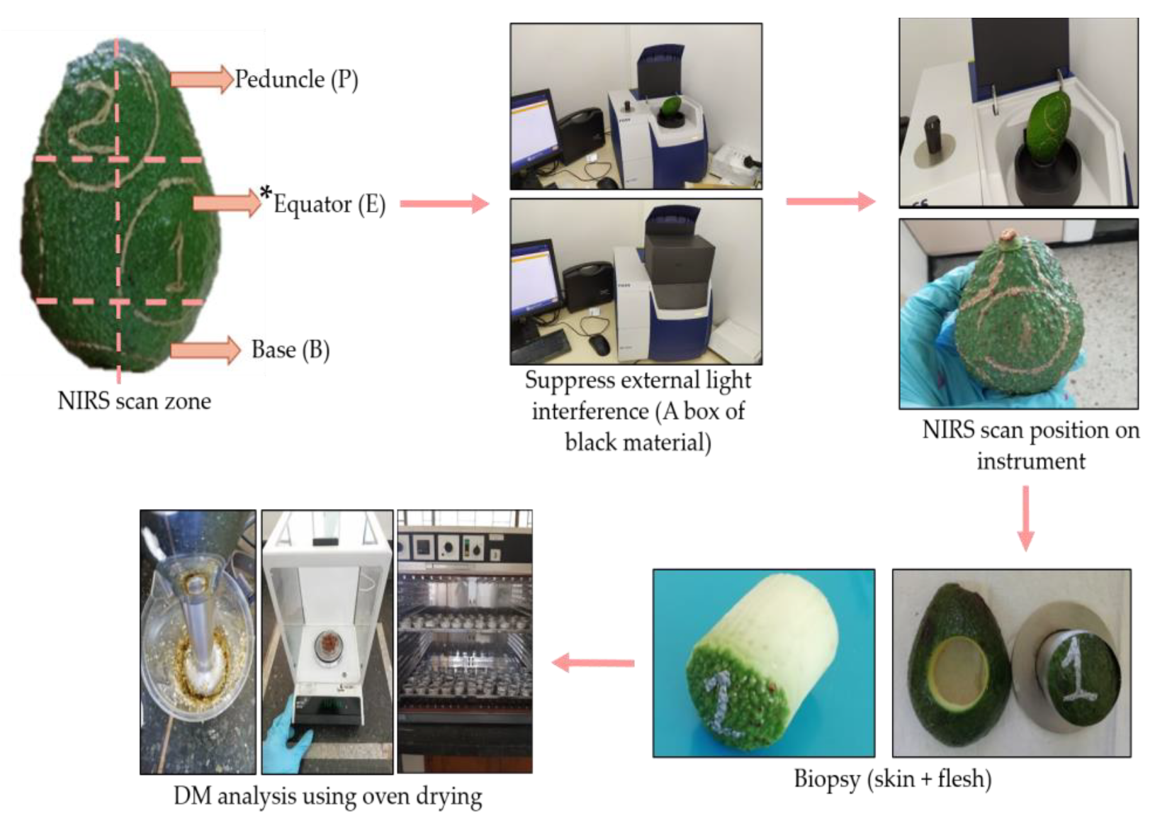Moreover, in Mexico, nondestructive studies were carried out with scans on the peduncle to obtain more reliable results than those evaluated in the equatorial zone due to the interference of the DM gradient present in the seed [14]. Despite efficient models developed for DM quantification, no focus has been placed on the robustness of these models according to the zone of the fruit. Therefore, the aim of this work was to determine a methodology to capture the variability presented within the same fruit using NIRS.

2. Materials and Methods

2.1. Avocado samples

For this study, ten Hass Avocado (Persea americana Mill cv. Hass) fruits were collected randomly in a packing house line (Pacific Fruits, Palmira Colombia). The fruits, freed of damage and diseases, were harvested at maturity with a commercial size of 18 (203 – 243g). NIR spectra analysis was collected in the CIAT facilities (International Center for Agriculture Tropical Palmira Colombia) in the Nutritional Quality Laboratory (NQL) and DM quantification was made, using the oven method, in the Palmira Research Center of Agrosavia (Colombia).

2.2. Spectroscopic measurement and data acquisition

The spectra were obtained using a near infrared FOSS DS 2500 spectrometer device (FOSS, DK-3400 Hilleroed, Denmark). Each fruit was analyzed in three zones, the peduncle, equator, and base (Figure 1). For each zone, three measurements were performed on each intact Hass avocado (peduncle, equator, and base). The fruit was placed on a round capsule sample holder with an external diameter of 5 cm and a quartz window with an internal diameter of 3.8 cm for spectral reading in reflectance mode. A box of black material was adapted in the NIRS scan zone of the equipment to avoid interference from external light (Figure 1). All reflectance NIR spectra were obtained at 2 nm intervals from 400 to 2500 nm in the wavelength range. Each spectrum consisted of 32 scans that were automatically averaged and recorded as log 1/reflectance (log 1/R). Spectral data were extracted with the WinISI Version 4.6.8 program (FOSS, DK-3400 Hilleroed, Denmark).

2.3. Dry matter analysis

The same area of the fruit scanned was labeled with metallic marker (Artline 990XF gold; Nagoya City, Japan), and then, a core of 3 cm in diameter perpendicular to the surface of the fruit (skin + flesh) was extracted using a steel corer (9 cores were taken per fruit). Next, the samples were processed with a blender to obtain a homogeneous extract. Samples were dehydrated using a hot air oven (UL 50, Memmert, Schwabach, Germany) at a temperature of 75 °C for 48 hours until reaching a constant weight [13]. The dry matter (DM) content was calculated based on Equation (1):

D M (%) = (\frac{W 1}{W 2}) * 100

(1)

where W1 refers to the weight of the oven-dried sample (g) and W2 is the weight of the wet avocado sample.

2.5. Data analysis

2.5.1. DM descriptive statistics and ANOVA

DM descriptive statistics and DM distribution (histogram) were calculated. ANOVA was performed to evaluate the effect of the 2 factors (fruit zones per fruit) and fruits on the level of DM content. The ANOVA was completed with a Newman‒Keuls (SNK: Student–Newman‒Keuls) test of means comparison with a confidence interval of 95%. All statistics were performed using XLSTAT software (Addinsoft (2023). XLSTAT statistical and data analysis solution. Paris, France. https://www.xlstat.com/fr).

2.5.2. Chemometric data analysis

Principal component analysis (PCA mean-centered) was performed with the raw data of the whole spectra. Cross-validation was performed by applying a random model with 20 segments using a singular value decomposition (SVD) algorithm.

Spectrum quality was evaluated using the root mean square (RMS) statistic [16,17]. The RMS statistic included in the WinISI software was used to calculate the agreement between the spectra within the Hass avocado fruit zone and between them. The RMSi was calculated for the 3 spectra acquired per zone of each fruit as follows (Equation 3):

R M S (i) = \sqrt{\sum_{j}^{P} \frac{{(\bar{X j} - X i j)}^{2}}{p}}

(3)

\bar{X} j = \frac{1}{n} \sum_{i}^{n} X i j

(4)

where n is the number of spectra compared (i range from 1 to n), p is the number of wavelengths (j range from 1 to p), Xij is the absorbance value of spectrum i at wavelength j and mean of absorbance of wavelength j (Equation 4).

2.5.3. Calibration

Prior to data modeling, preprocessing methods were applied to correct light scattering and reduce the changes in light path length. First, GAP derivative preprocessing was used with the 1st derivative order with a GAP size of 5 (number of points). Second, a detrending transformation was performed to remove nonlinear trends. Detrending was performed with a polynomial order of 2.

A partial least squares regression (PLS) was performed with the transformed dataset (the algorithm used kernel, validation method: cross-validation, random with 20 segments). Different calibration models were used on three, two, and one spectrum per fruit zone.

2.5.4. Projection

The PCA models were employed to build projections of the spectra of the replicates in each zone. The chemometrics data analysis was performed using Unscrambler software (Unscrambler X Version 10.5. 1, CAMO, Oslo, Norway).

3. Results and Discussion

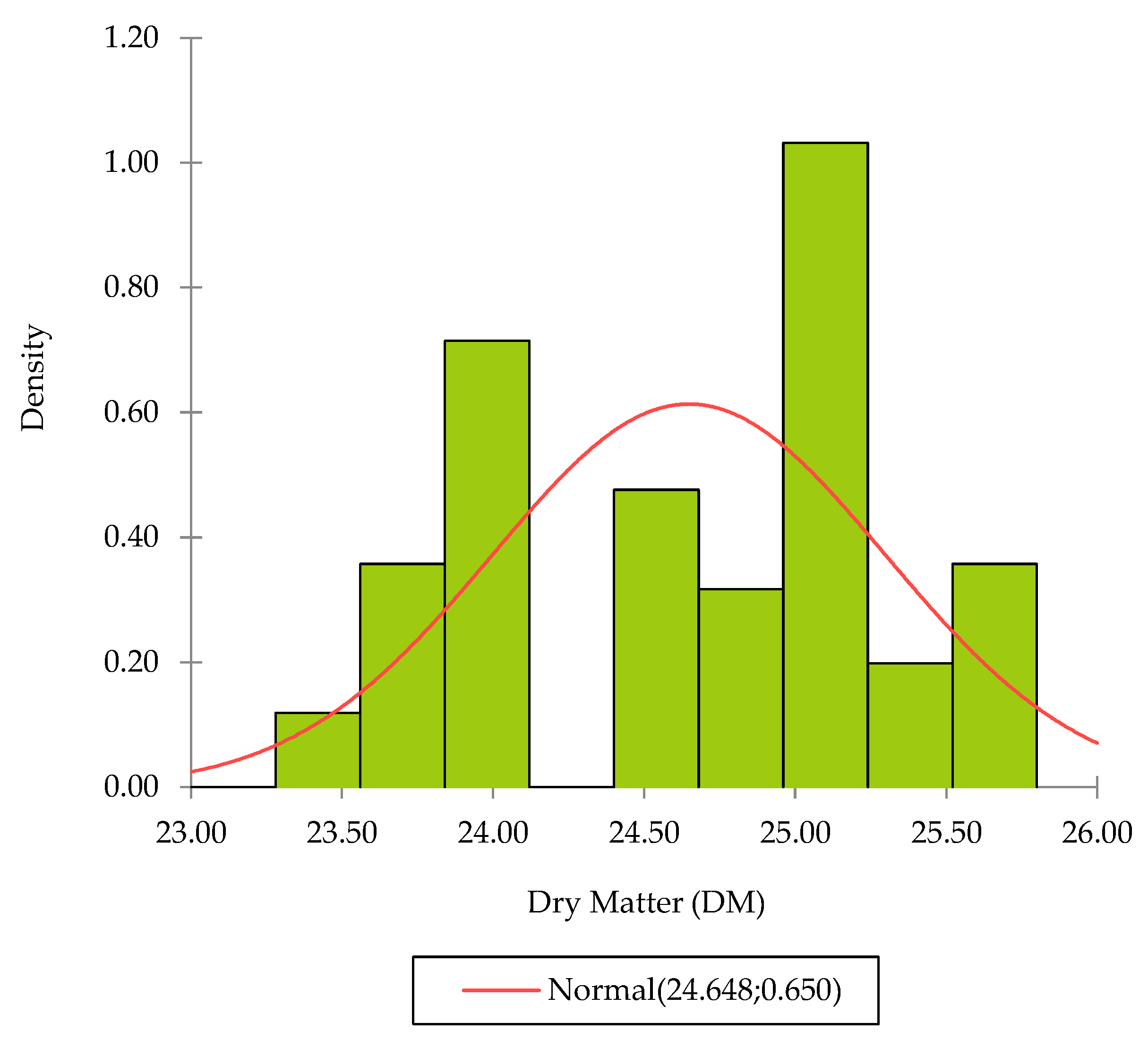
The DM values range between 23.41% and 25.73%, with an average value of 24.65% and a standard deviation of 0.65%. The repartition of the values shows two populations and is in concordance with the discussion that will be presented below (Figure 2). This repartition is due to fruits F1, F7, and F9, which present average DM contents lower than 24%.

The ANOVA (two factors: zone and fruit) of the DM shows (Table 1) evidence that there is a fruit effect and a zone effect inside Hass avocado samples, with a “fruit” effect more significant than a zone effect based on type III errors.

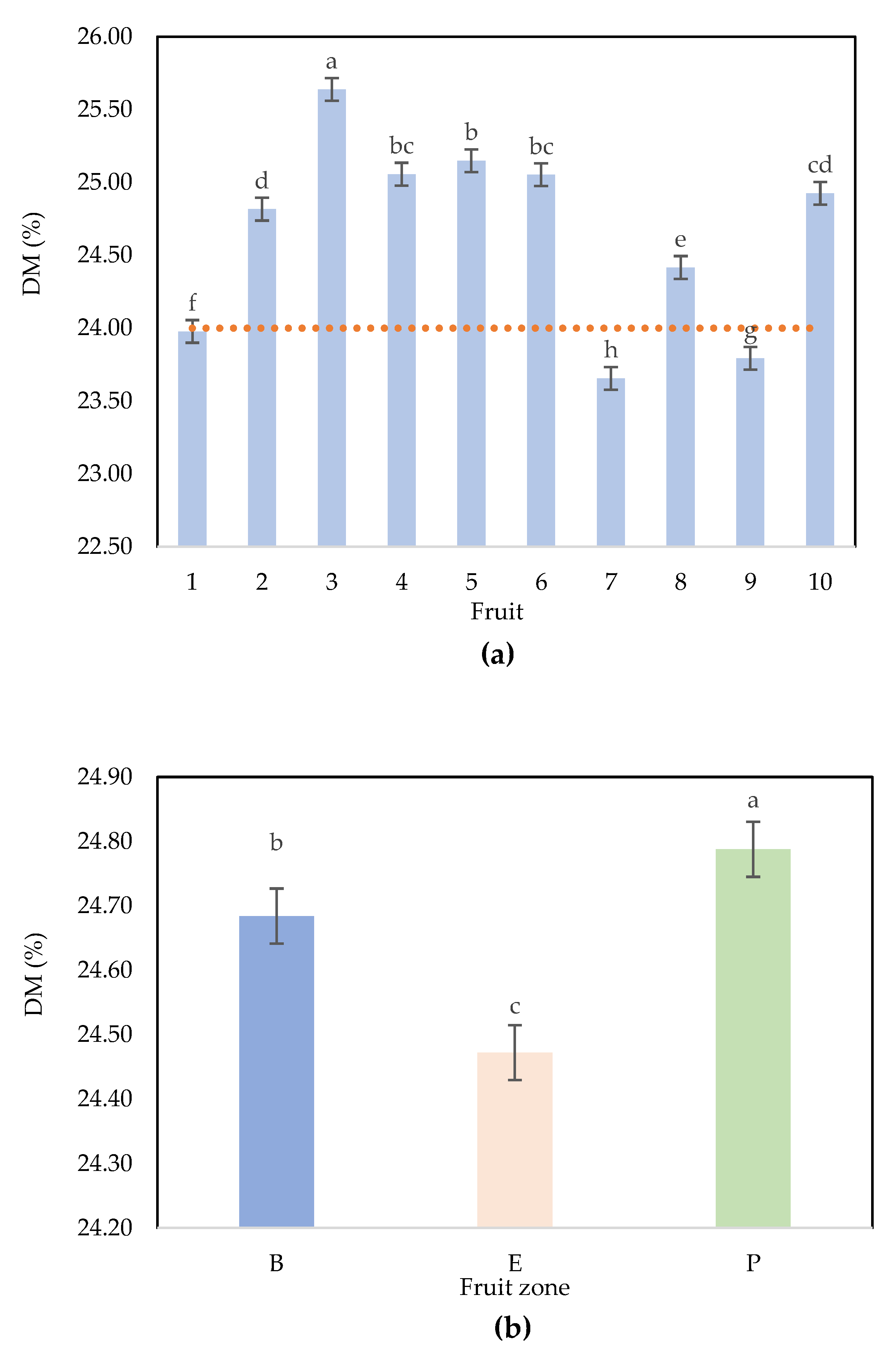
A Newman‒ Keuls (SNK) test comparing the differences between the factor “fruit” with a confidence interval of 95% confirms that F3, F8, F1, F9, and F7 are different from all other fruits and that F4, F5, and F6 are not significantly different (same DM), and the same result occurs for F4, F6, and F10 and for F10 and F2 (Figure 3a). A Newman‒Keuls (SNK) test comparing the differences between the levels of “zone” with a confidence interval of 95% confirms that the 3 zones are significantly different, with average values ranging from 24.47% (equator), 24.68% (base) and 24.79% (peduncle) (Figure 3b).

There is a DM gradient within the fruit, with higher DM content on the peduncle followed by the equator and base zones. The variability within the fruit was shown by Phetsomphou (2000) and Wedding et al. (2010) [19,20] not only in the P, E, and B zones but also in the outer, middle, or inner fruit. Therefore, this gradient affects the robustness of both destructive and nondestructive analyses for DM quantification. The literature does not show a clear trend in the direction of the gradient. Moreover, there is a lack of information that explains the phenomenon well. Schroeder (1985) indicated that these gradients could be related to complex fruit development physiology [9]. There are many differences in structure and metabolic activity that eventually are demonstrated within the avocado fruit. Moreover, the gradient within the fruit and the variability between fruits increase the difficulty of guaranteeing the minimum dry matter needed to export fruits. According to Rodríguez et al. (2018), almost 80% of fruit samples must have a DM higher than 24% to have good postharvest quality in the international market. The results show that the samples in this study have 70% to 24% DM [18].

Regarding methodologies applied to build NIRS predictive models of Hass avocado DM estimation, almost all the authors scanned the fruit in the equatorial zone two or more times [5,11,15,21]. In other fruits, the same methodology has been employed in that only the equator zone is scanned [22,23]. Although the DM gradient within the fruit has been published for Hass avocados, NIRS models are considered destructive analyses of the outer (0.5-1.0 cm) layer of the mesocarp and skin; thus, the analysis could have a bias with respect to the whole fruit DM content. P.P. Subedi and K.B. Walsh (2020) found a difference of 4% in DM between the outer and inner parts of Hass avocados [15]. The authors developed predictions despite this high variation. In terms of fruit development, 4% dry matter implies a difference in fruit age of almost 40 days according to Rodríguez et al. (2018) [18]. We found a nonsystematic bias in the dry matter of +/- 4% in the analysis of the DM with commercial, portable NIRS in Colombia (data not shown). Therefore, these devices do not allow efficient sorting of fruit in orchards or packing houses.

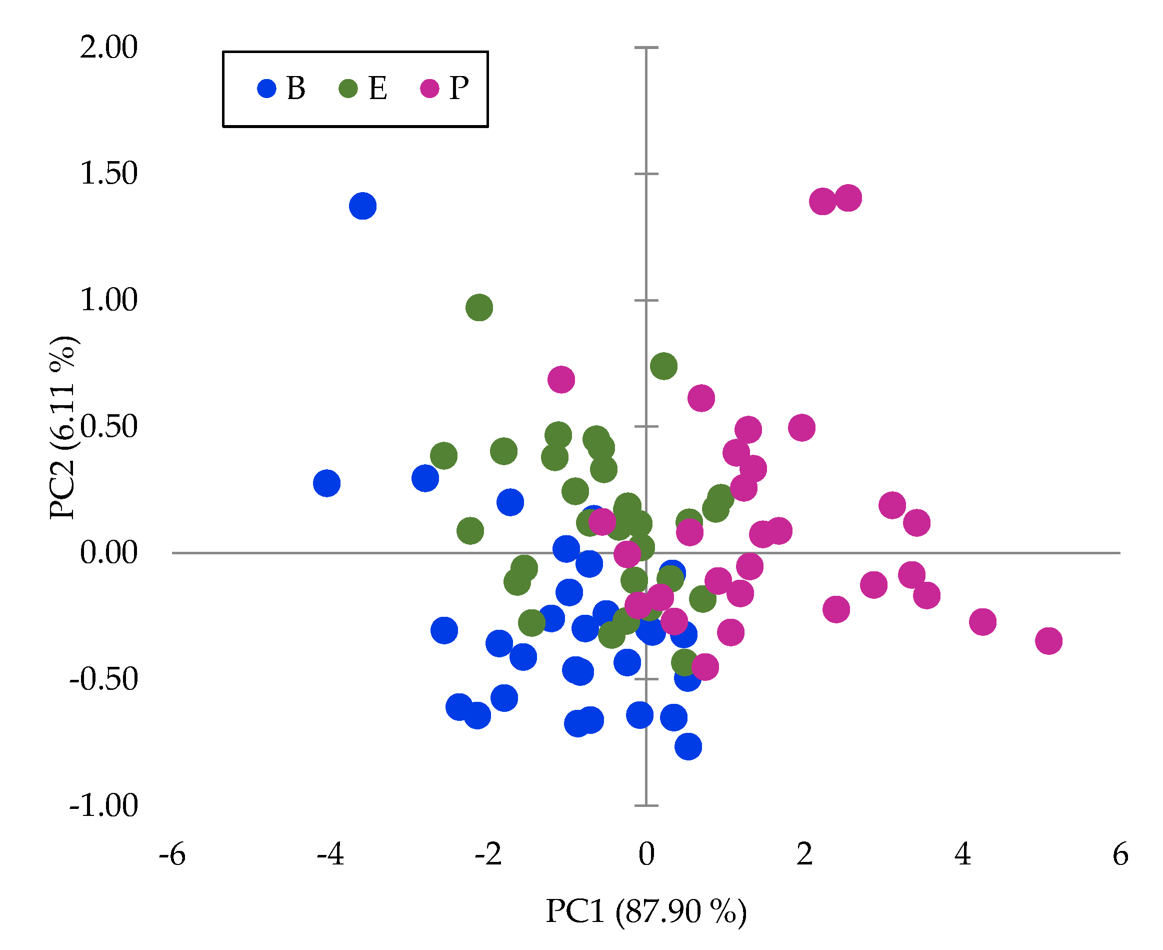
PCA was performed on the raw data, log (1/R), for the whole wavelength range, and the dimension of the input matrix is n = 90 and p = 1050. The first two PCs explained 94% of the total inertia, and 88% and 6%, respectively. The presentation of the sample scores for the first two PCs highlights differences between zones (Figure 4), which indicates that there is high variability within spectra due to the zone of the fruits. These groups have not been reported before, although there are many publications on the use of NIRS technology to analyze DM in Hass avocados.

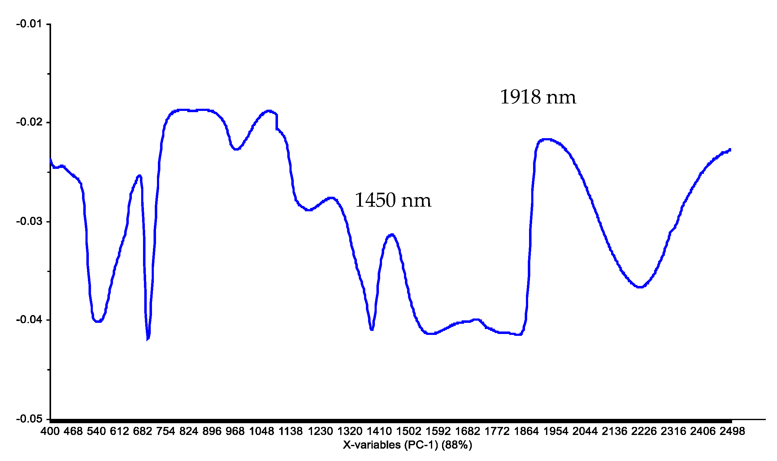
The loadings associated with PC1 show two main peaks in the NIR region: 1450 nm and 1918 nm, which correspond to water (O-H) absorption bands (Figure 5). The results agree with those of other works that indicated that for Hass avocados, the main peaks are closely associated with the H-O-H stretching modes of water [5].

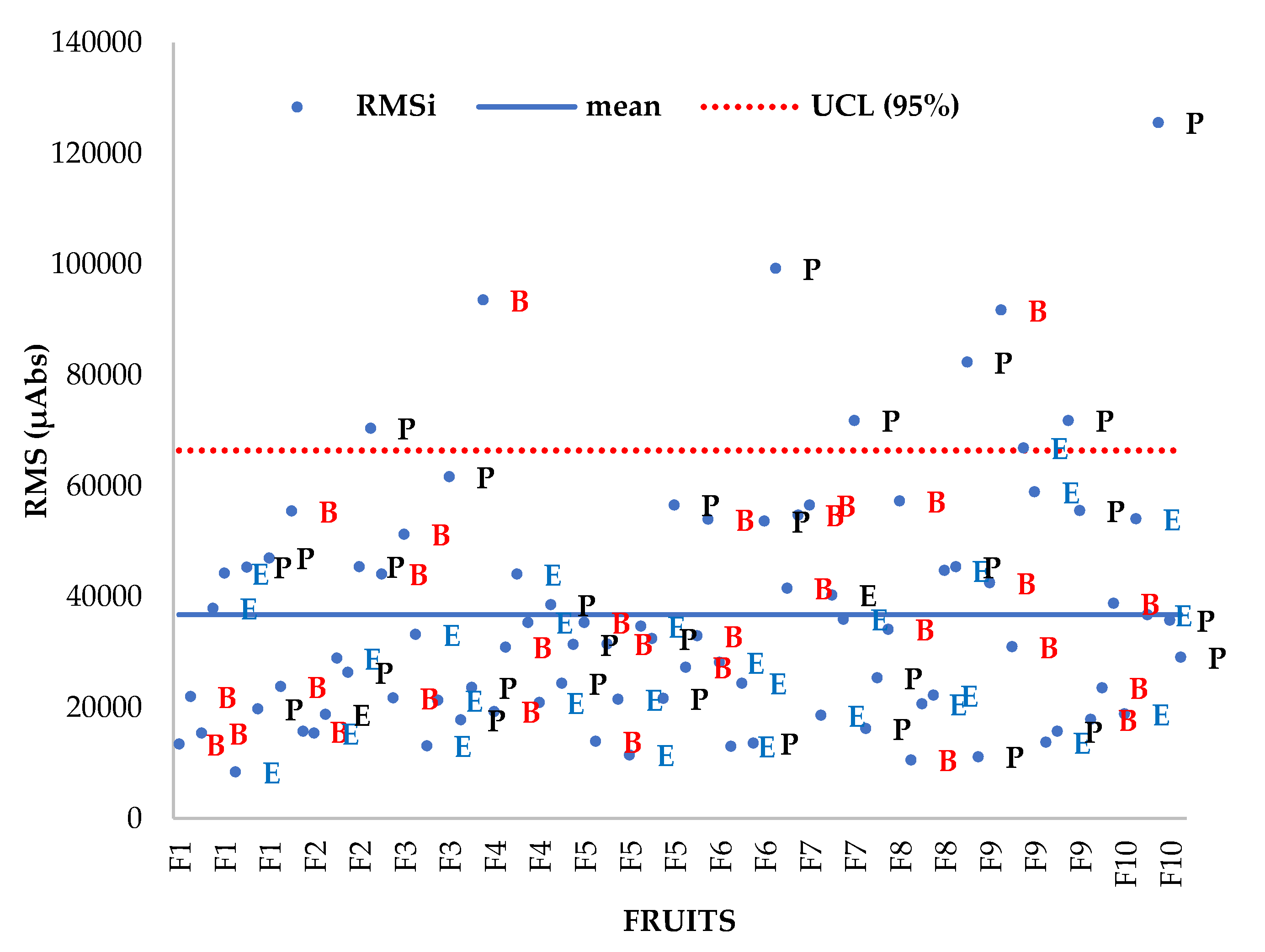
The RMSi for each zone (Figure 6) shows that despite some outlier spectra (with high RMS values), all RMSi values are of the same order.

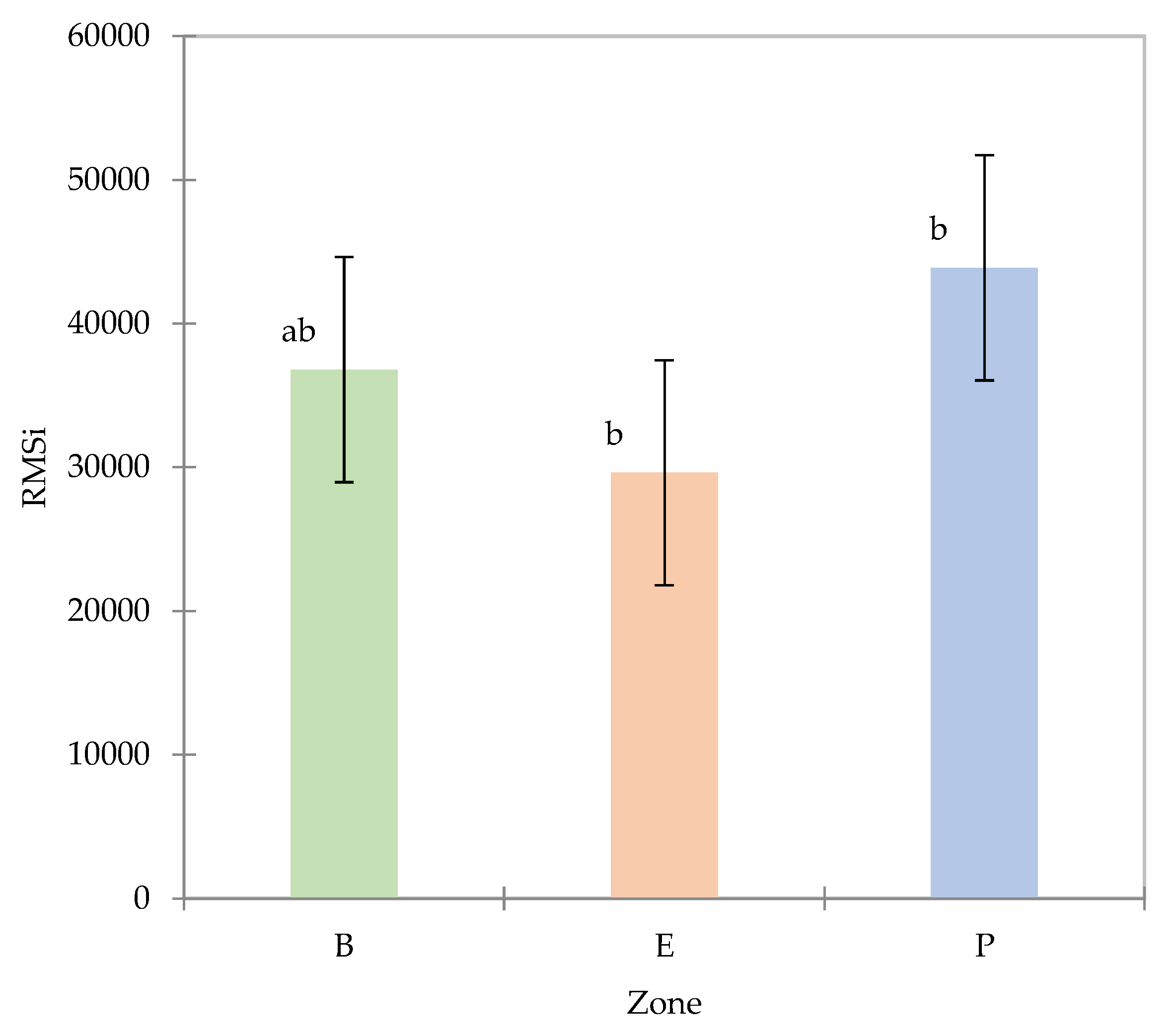
The RMSi average values are given per zone (for all the fruit), an ANOVA on the RMSi values with zone as factor confirms that there is a significant effect (α = 5%) of the zone of the fruit on spectra variability (Pr>F = 0.043), the contrast test (Newman‒Keuls, SNK) confirms a difference between peduncle and equator, and no difference between peduncle and base and no difference between base and equator occur (Figure 7).

These results associated with DM content observations suggest that at least one spectrum per zone is reasonable for determining the variability in the whole fruit.

The RMSi method of calculating dispersion is commonly used in NIRS analysis and is known as the root mean square error or root mean square deviation. It is a measure of the variability in a group of spectra that are supposed to be similar. Therefore, this descriptor indicates spectral similarities between avocado zones. This study highlights the existing spectral variability between fruit zones. Therefore, at least one scan must be performed per zone to capture the whole fruit variability as will be discussed in section on the multivariate analysis.

Calibration based on three spectra per zone

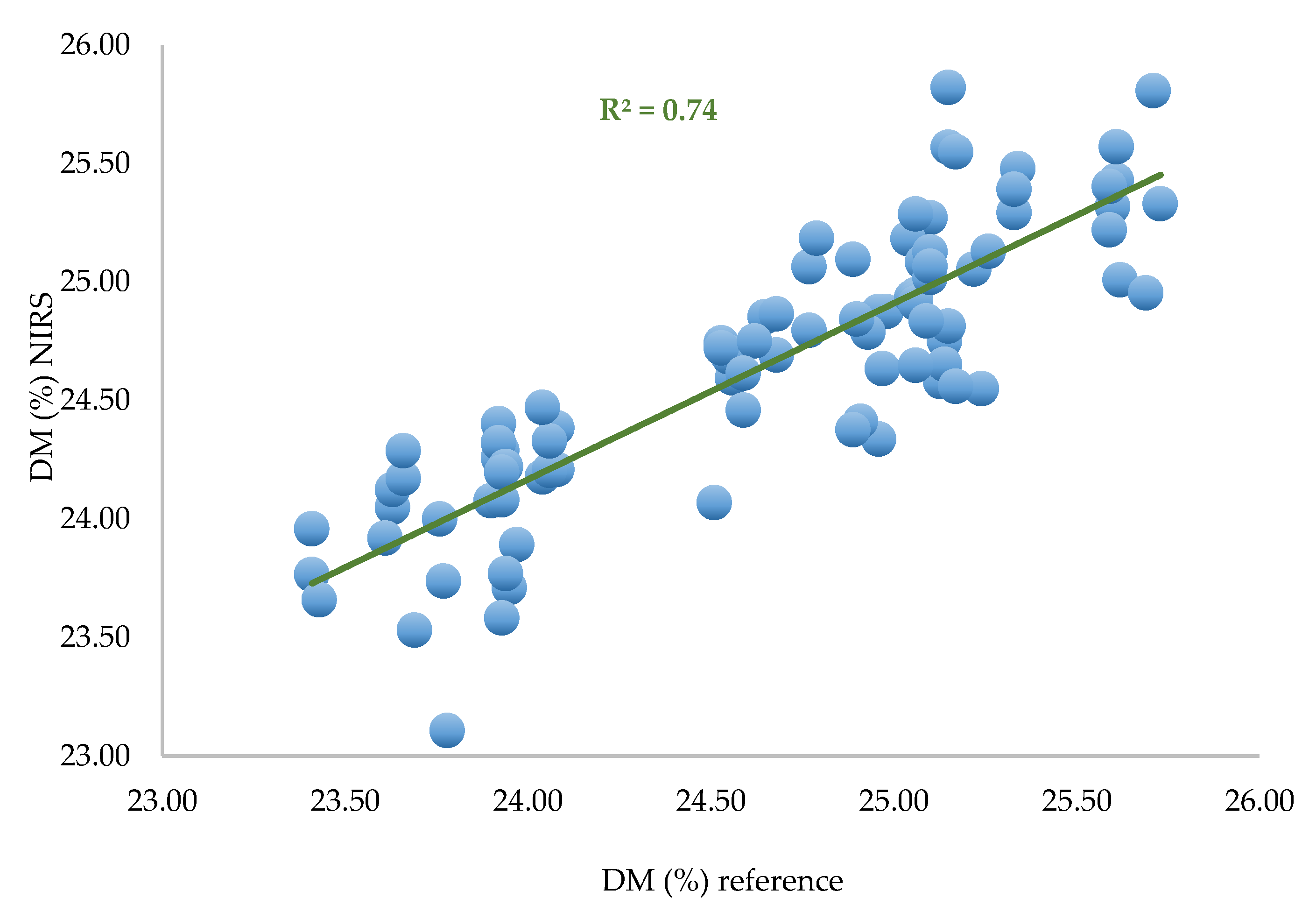
A first calibration was performed with all the spectra (90) and all DM values (90), and the best pretreatment is the first derivative (gap derivative, gap size = 5) and a correction detrending (second-order polynomial). PLS regression is used for calibration.

Table 2. PLS equation performances for three spectra per zone.

N	R² calibration	SEC	RMSEC	R² Validation	RMSECV	SECV	# PLS
90	0.743	0.329	0.328	0.522	0.4526	0.455	8

SEC: Standard Error of Calibration; RMSEC: Root Mean Squared Error of Calibration; RMSECV: Root Mean Square Error of Cross Validation; SECV: Standard Error of Cross Validation.

Figure 8. Predicted DM versus laboratory DM calculated with PLS regression based on all data (n = 90).

Calibration based on two spectra per zone

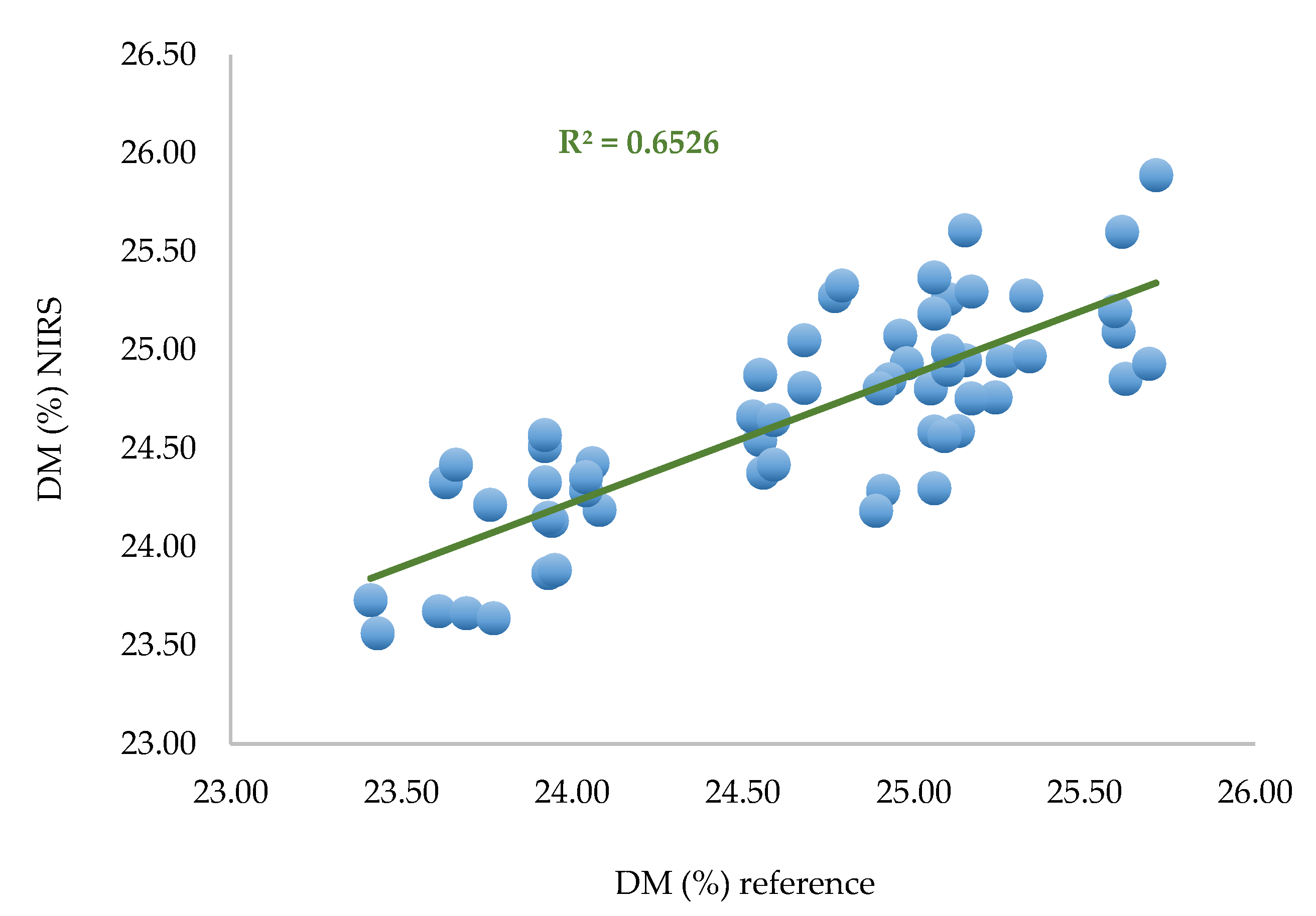
A calibration based on PLS regression with the same pretreatments was performed on 60 samples corresponding to two spectra per zone per fruit.

Table 3. PLS equation performances for two spectra per zone.

N	R² calibration	SEC	RMSEC	R² Validation	RMSECV	SECV	# PLS
60	0.653	0.384	0.382	0.284	0.577	0.582	7

SEC: Standard Error of Calibration; RMSEC: Root Mean Squared Error of Calibration; RMSECV: Root Mean Square Error of Cross Validation; SECV: Standard Error of Cross Validation.

In the learning step, the performances are quite similar (SEC, R²) to those observed for the calibration with the whole set of data. The performances decrease during validation (RMSECV = 0.577%).

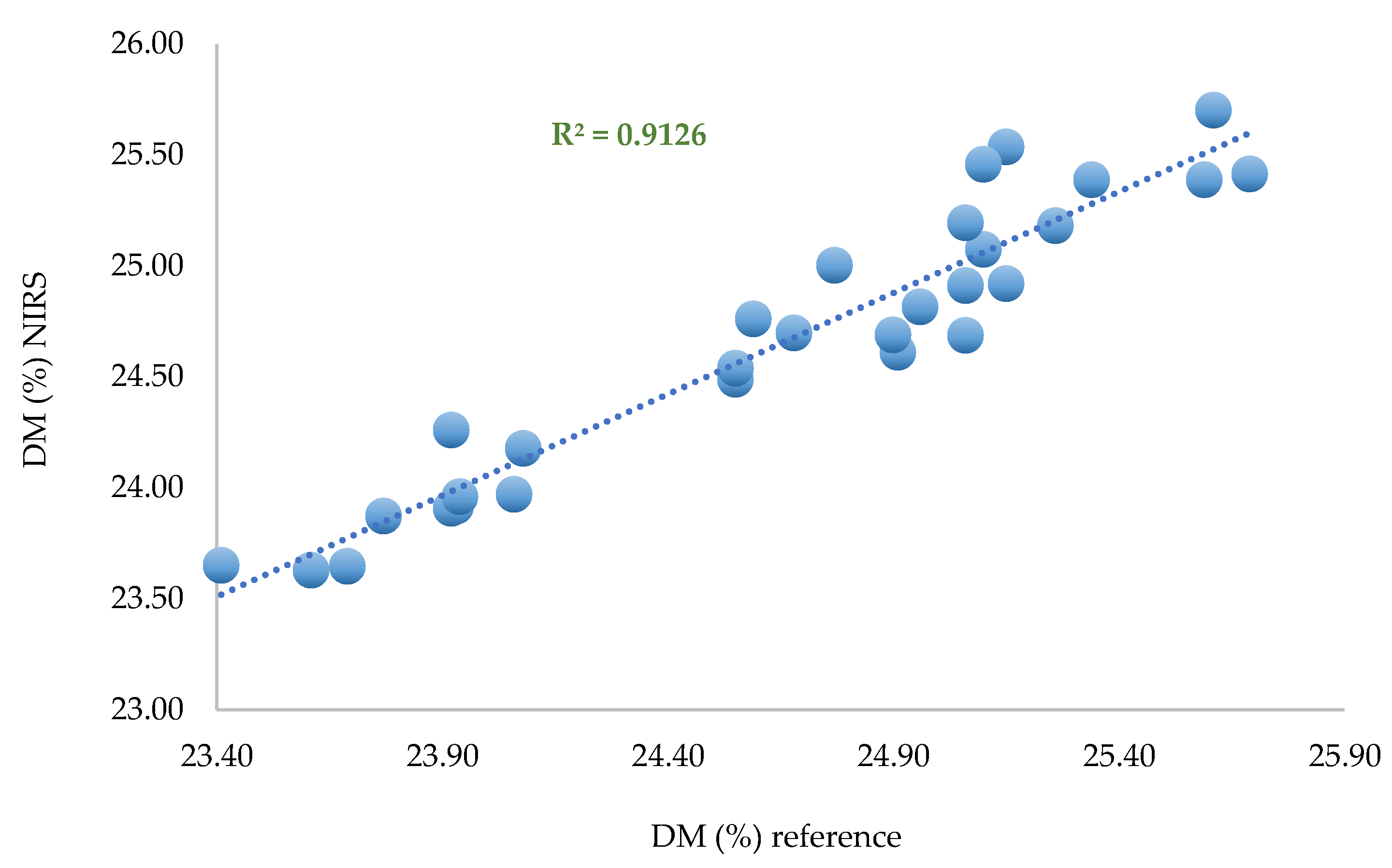
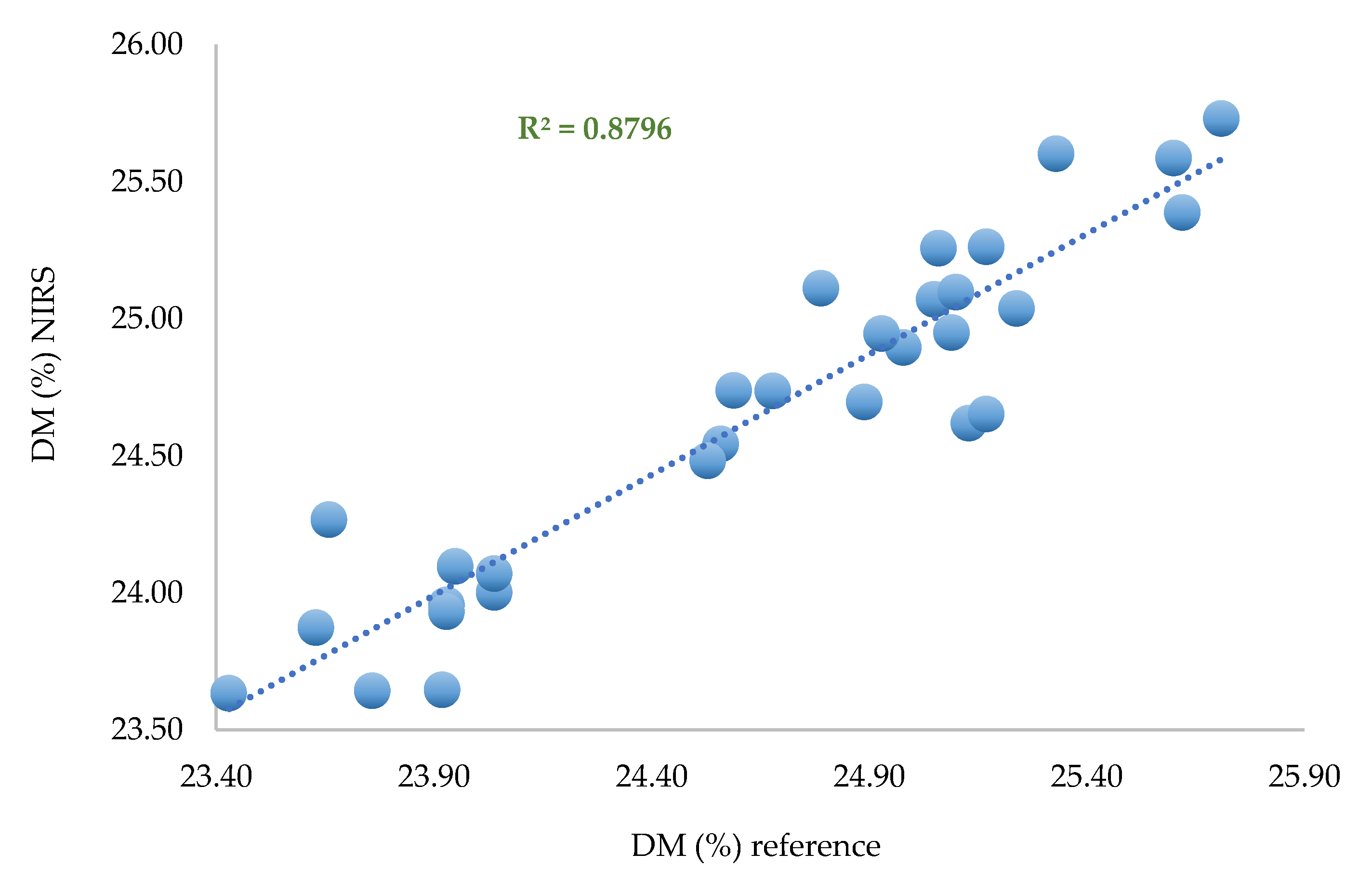
Figure 9. Predicted DM versus laboratory DM. PLS regression based on selected data (n = 60). Two spectra per zone per fruit.

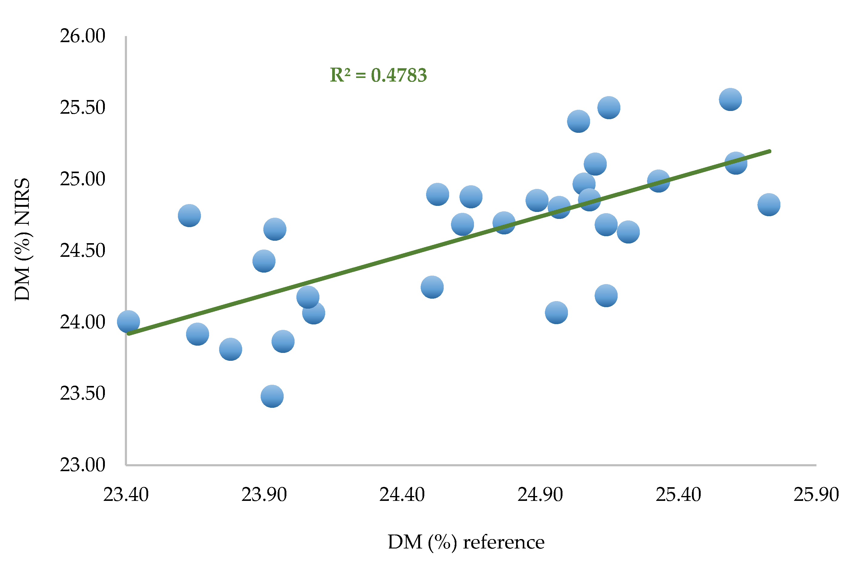
This model was used to predict the set of remaining spectra (30) corresponding to one spectrum per zone per fruit.

Table 4. Prediction parameter performances.

N	R²	SEP	RMSEP	slope	Bias
30	0.478	0.479	0.474	0.55	-0.047

SEP: Standard Error of Prediction, RMSEP: Root Mean Squared Error of Prediction.

Figure 10. Predicted values versus laboratory values for the 30 remaining spectra (one per zone per fruit).

The SEP observed in the remaining 30 spectra is SEP = 0.479%, which is satisfactory regarding the average DM content of the fruit (24.65%). This result indicates that 2 spectra per zone could be enough to build an efficient and robust model for dry matter quantification.

Calibrations based on one spectrum per zone per fruit

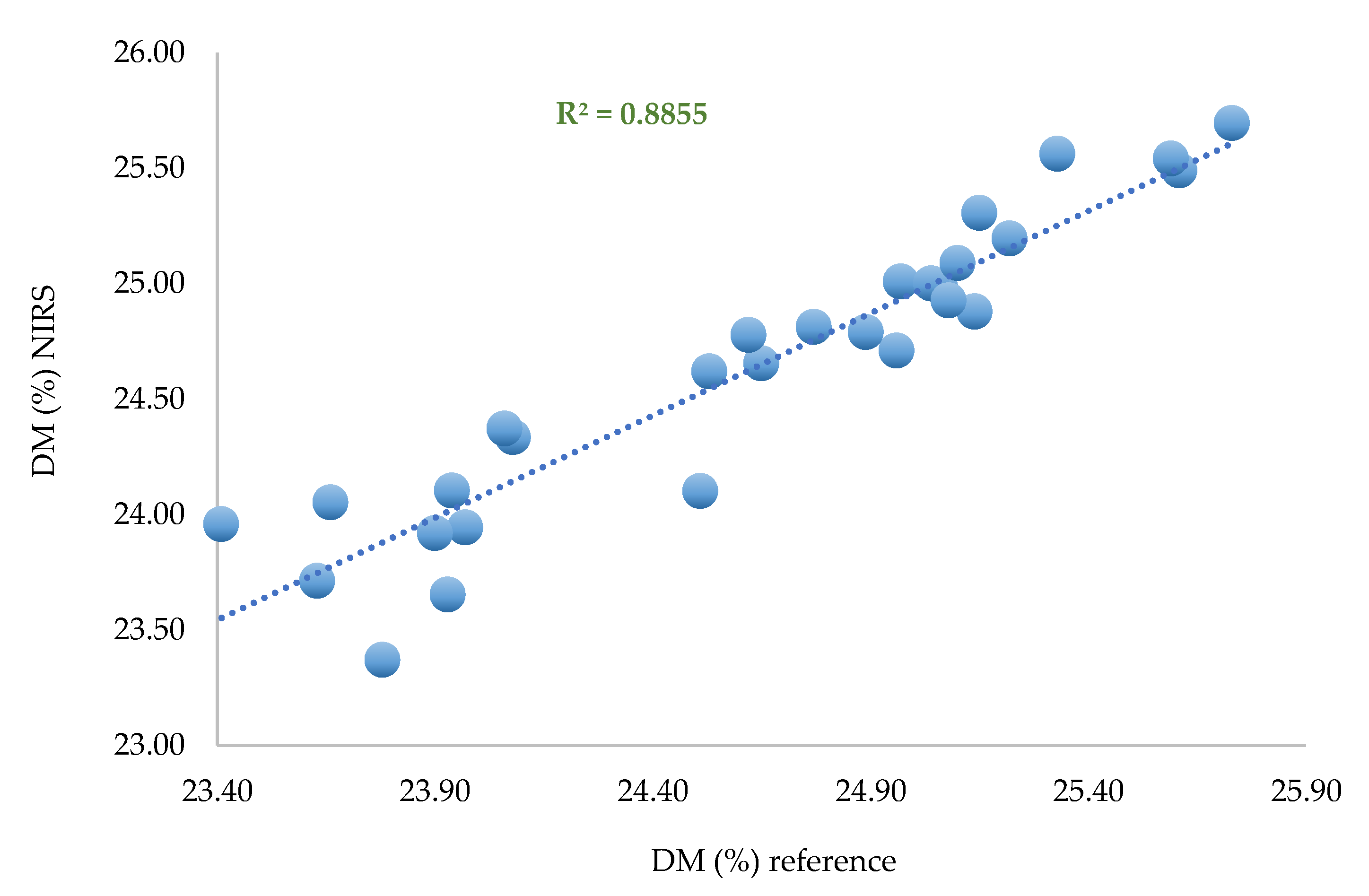
Three calibrations based on PLS regression with the same pretreatments were performed on 30 samples corresponding to one spectrum per zone per fruit. One calibration was performed per replicate set.

Figure 11. Predicted values versus laboratory values for 30 spectra (replicate n°1 per zone).

Figure 12. Predicted values versus laboratory values for 30 spectra (replicate n°2 per zone).

Figure 13. Predicted values versus laboratory values for 30 spectra (replicate n°3 per zone).

Table 6. The prediction parameter performance.

Calibration	Prediction set	N	R²	SEP	RMSEP	slope	Bias
R1	R2_R3	60	0.578	0.424	0.420	0.588	-0.009
R2	R1_R3	60	0.530	0.454	0.450	0.614	-0.016
R3	R1_R2	60	0.166	0.777	0.782	0.479	-0.130

SEP: Standard Error of Prediction, RMSEP: Root Mean Squared Error of Prediction.

These models are used to predict the 3 sets of remaining spectra (30) corresponding to two spectra per zone per fruit.

The calibration using the third replicate performs worse than the two others in terms of prediction. Nevertheless, the average standard error of prediction observed using each subset of replicates is 0.551%, which is a promising result. Most likely, some of the spectra of replicate 3 are noisy, which degrades the performance of the model but justifies using at least one spectrum per zone to be representative and minimize the effect of "atypical" spectra.

Although it has been well documented by using destructive analysis that there is a Hass avocado DM gradient within the whole fruit, NIR applications for Hass avocado are focused on building PLS models with the NIRS spectra of the fruit equatorial zone. These models could have a bias that could affect the DM prediction, and the fruit shipped to different areas could have internal quality issues.

This work demonstrates that one calibration per replicate set has a good DM prediction ability according to the fit statistics shown in Table 5. It is possible to predict the DM variability within a whole fruit with an NIRS scan per zone. The results are in agreement with those of other works that have used NIR spectroscopy to predict fruit quality and composition. Specifically, some studies have focused on the effect of different fruit orientations, such as the stem-calyx axis and equator, on the quality of acquired spectra [24,25,26,27]. The results of the research show that measurement orientation on spectra greatly affects the prediction accuracy of lignin, soluble solids, and acidity content in pears, peaches, kiwifruit, and apples, respectively.

PCA projections

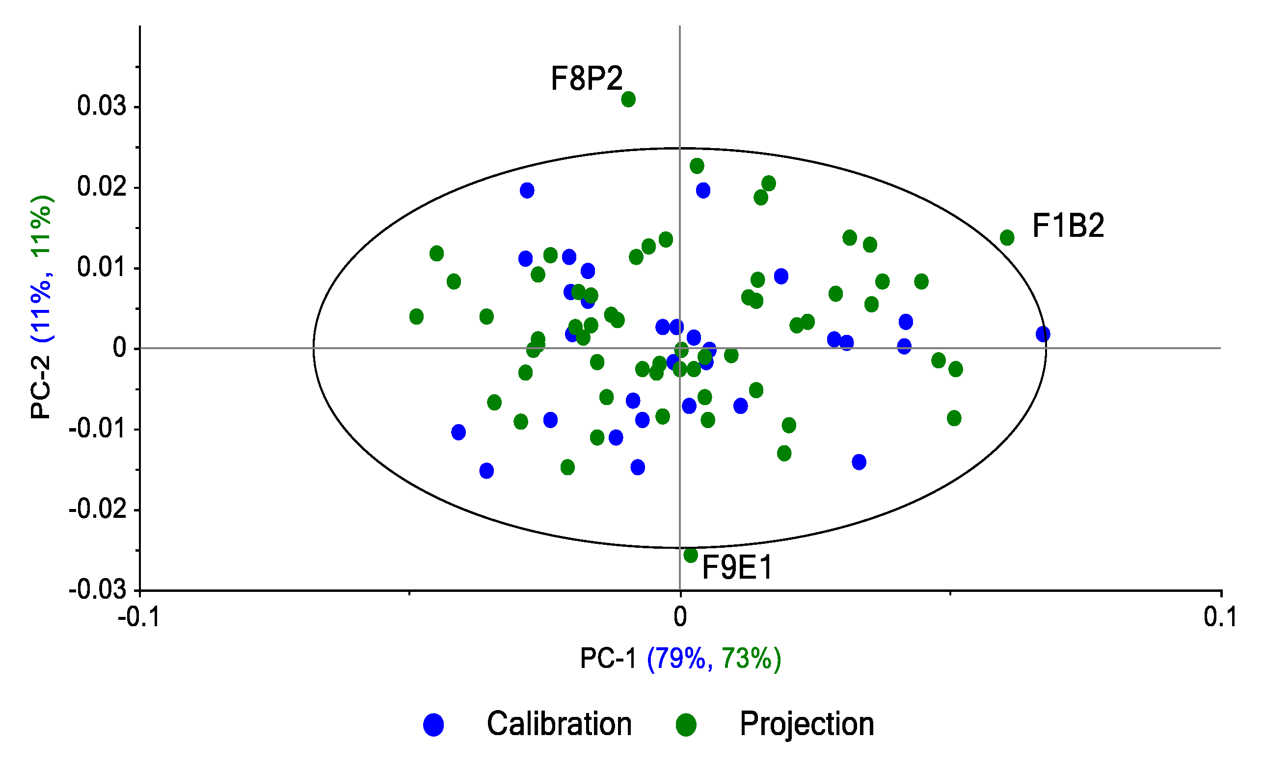
NIRS users also have difficulties identifying and detecting samples that are considerably different from the majority of the remaining samples, which are known as outliers. Based on the literature and common NIRS practices, outlier data can be identified by projecting spectral data onto principal component analysis (PCA) and applying the Hotelling’s T² ellipse, as presented in Figure 14. Data lying outside the ellipse are potential outliers [28].

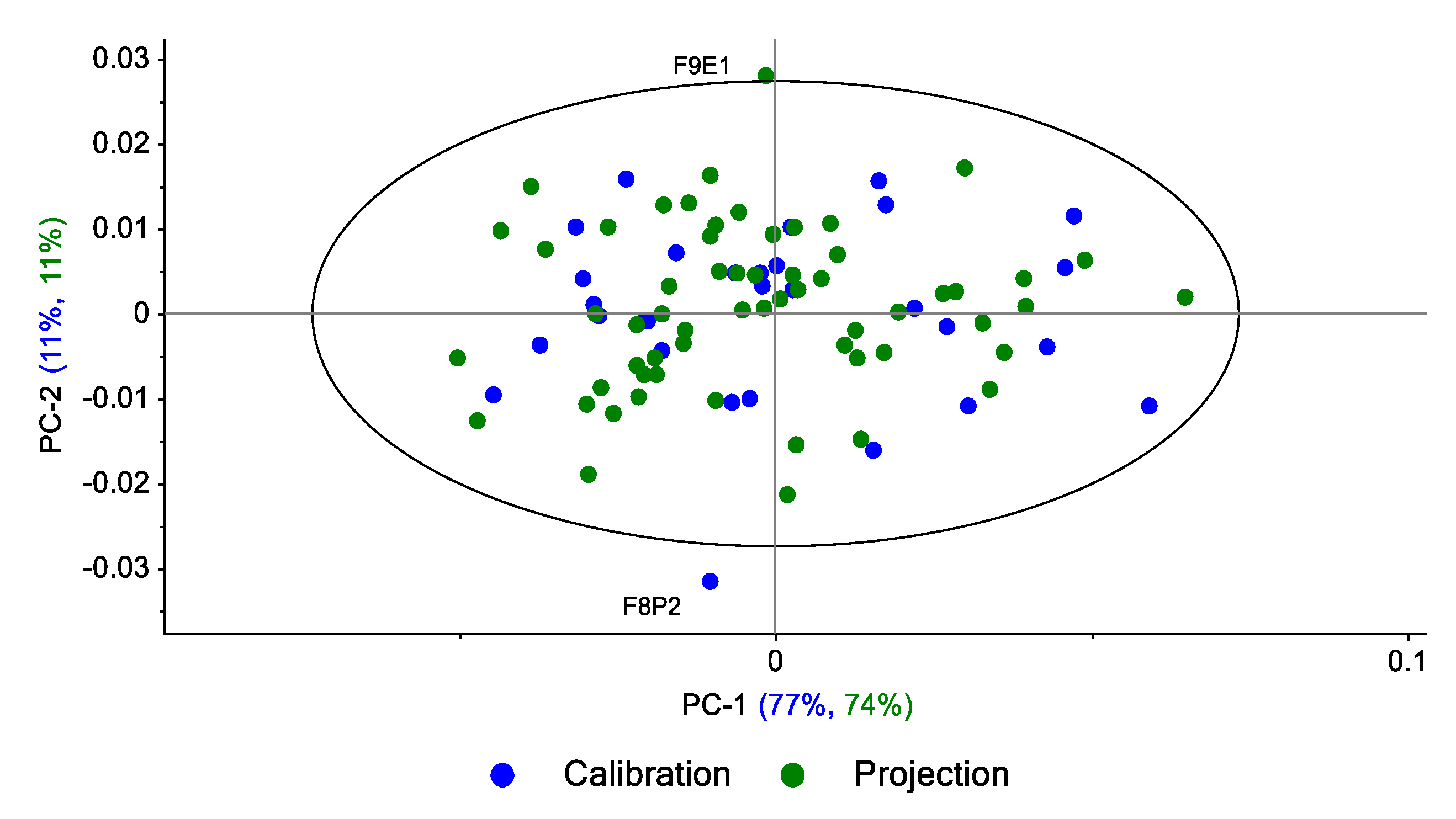
The projection of the spectra of replicates 1 and 2 per zone on the main plan (PC1 vs. PC2) calculated on the spectra of replicate 3 shows (Figure 14) that 84% of the variance in the R1-R2 spectra is explained by the R3 spectra. Three spectra are outside the 95% confidence ellipse.

The same approach was performed by projection of the R2 and R3 replicates (60 spectra) on the subspace defined by calculating PCs from R1 replicate spectra (n = 30); 84% of the variance in the R1-R3 spectra is explained by the R1 spectra (Figure 15). Three spectra are outside the 95% confidence ellipse: one from R2 and one from R3. The third spectrum is from R1, which indicates that this spectrum is an outlier in the R1 set (atypical spectrum).

The same approach was performed by the projection of the R1 and R3 replicates (60 spectra) on the subspace defined by the calculation of the PCs from the R2 replicate spectra (n = 30). Eighty-five percent of the variance of the R1-R3 spectra is explained by the R2 spectra. Two spectra are outside the 95% confidence ellipse: one from R1 and the other from the R2 set, which means that this spectrum is an outlier in the R2 set (atypical spectrum).

Figure 16. Projection of the 60 spectra of the replicates 1 and 3 per zone on the main plain of the PCA calculated on 3 spectra of R2 (95% confidence ellipse). Fruit zone: B: base, E: equator, P: peduncle. F: Fruit.

These results based on PCA models and projections show that spectral variability per area can be captured with a single spectrum. For the 3 models, less than 5% of the projected samples can be considered outliers with Hotelling’s T² distances close to the limit.

5. Conclusions

The destructive laboratory determination of DM contents of the different zones of the fruit confirms the heterogeneous repartition of dry matter within the fruit. With a significant effect of fruit zone, the DM ranged from 24.47% (equator) to 24.68% (base) and 24.79% (peduncle).

The experiment demonstrates the ability of NIRS to predict the dry matter content of intact whole avocado fruits with a standard error of cross-validation of 0.455%.

The different tests using PLS regression or PCA projection of the replicate subsets indicate that it is possible to use 3 spectra per fruit, one per zone with a reasonable representativeness of the fruit.

Author Contributions

P.R.: Conceptualization, methodology, data curation, writing–original draft, formal analysis, supervision, project administration, and funding acquisition. J.V.: Methodology and writing–original draft. L.L.: methodology and writing–original draft. T.T.: Conceptualization, methodology, and writing–original draft. F.D.: Conceptualization, methodology, data curation, writing–original draft, formal analysis, and supervision. All authors have read and agreed to the published version of the manuscript.

Funding

This research and the APC have been funded by the Sistema General de Regalías-SGR of the De-partment of Cauca (Colombia), under the Special Cooperation Agreement for Research No. 068 of 08/10/2018. The OCAD of the FCTeI designated the Corporación Colombiana de Investigación Agropecuaria-Agrosavia as the executing public entity of the project identified with the BPIN code 2018000100010 called "Development and validation of technologies to increase the produc-tivity of the Hass Avocado crop in the Department of Cauca".

Data Availability Statement

The data that support the findings of this study are available from the corresponding author upon reasonable request.

Acknowledgments

The authors express their gratitude to the orchard growers, the support team, and Palmira Research Centers (Agrosavia) for support in the technical execution of the study and the Department of Cauca (Colombia) for the financial funding.

Conflicts of Interest

The authors declare no conflict of interest. The funders had no role in the design of the study; in the collection, analyses, or interpretation of the data; in the writing of the manuscript; or in the decision to publish the results.

Abbreviations

Abbreviations	Meaning
NIRS	Near Infrared Spectroscopy
DM	Dry Matter
OC	Oil Content
PCA	Principal Component Analysis
PLS	Partial Least Squares
SNK	Student Newman-Keuls
SVD	Singular Value Decomposition
GAP	Gap Difference Method
RMS	Root Mean Squared
RMSEC	Root Mean Squared Error of Calibration
RMSECV	Root Mean Square Error of Cross Validation
RMSEP	Root Mean Squared Error of Prediction
SEC	Standard Error of Calibration
SECV	Standard Error of Cross Validation
SEP	Standard Error of Prediction

References

Bill, M.; Sivakumar, D.; Thompson, A.K.; Korsten, L. Avocado Fruit Quality Management during the Postharvest Supply Chain. Food Reviews International 2014, 30, 169–202. [Google Scholar] [CrossRef]
Rivera, S.A.; Ferreyra, R.; Robledo, P.; Selles, G.; Arpaia, M.L.; Saavedra, J.; Defilippi, B.G. Identification of Preharvest Factors Determining Postharvest Ripening Behaviors in ‘Hass’ Avocado under Long Term Storage. Sci Hortic 2017, 216, 29–37. [Google Scholar] [CrossRef]
Escobar, J. V.; Rodriguez, P.; Cortes, M.; Correa, G. Influence of Dry Matter as a Harvest Index and Cold Storage Time on Cv. Hass Avocado Quality Produced in High Tropic Region. Informacion Tecnologica 2019, 30, 199–210. [Google Scholar] [CrossRef]
Lee, S.K.; Young, R.E.; Schiffman, P.M.; Coggins, C.W. Maturity Studies of Avocado Fruit Based on Picking Dates and Dry Weight; 1983; Vol. 108(3):390-394.
Olarewaju, O.O.; Bertling, I.; Magwaza, L.S. Non-Destructive Evaluation of Avocado Fruit Maturity Using near Infrared Spectroscopy and PLS Regression Models. Sci Hortic 2016, 199, 229–236. [Google Scholar] [CrossRef]
Nicolaï, B.M.; Beullens, K.; Bobelyn, E.; Peirs, A.; Saeys, W.; Theron, K.I.; Lammertyn, J. Nondestructive Measurement of Fruit and Vegetable Quality by Means of NIR Spectroscopy: A Review. Postharvest Biol Technol 2007, 46, 99–118. [Google Scholar] [CrossRef]
Lin, H.; Ying, Y. Theory and Application of near Infrared Spectroscopy in Assessment of Fruit Quality: A Review. Sens Instrum Food Qual Saf 2009, 3, 130–141. [Google Scholar] [CrossRef]
Walsh, K.B.; Blasco, J.; Zude-Sasse, M.; Sun, X. Visible-NIR ‘Point’ Spectroscopy in Postharvest Fruit and Vegetable Assessment: The Science behind Three Decades of Commercial Use. Postharvest Biol Technol 2020, 168. [Google Scholar] [CrossRef]
Schroeder, C.A. Physiological Gradient in Avocado Fruit; 1985; Vol. 69.
Woolf, A.; Clark, C.; Terander, E.; Phetsomphou, V.; Hofshi, R.; Arpaia, M.L.; Boreham, D.; Wong, M.; White, A. 2003.
Wedding, B.B.; Wright, C.; Grauf, S.; White, R.D.; Tilse, B.; Gadek, P. Effects of Seasonal Variability on FT-NIR Prediction of Dry Matter Content for Whole Hass Avocado Fruit. Postharvest Biol Technol 2013, 75, 9–16. [Google Scholar] [CrossRef]
Blakey, R.J. Evaluation of Avocado Fruit Maturity with a Portable Near-Infrared Spectrometer. Postharvest Biol Technol 2016, 121, 101–105. [Google Scholar] [CrossRef]
Ncama, K.; Magwaza, L.S.; Poblete-Echeverría, C.A.; Nieuwoudt, H.H.; Tesfay, S.Z.; Mditshwa, A. On-Tree Indexing of ‘Hass’’ Avocado Fruit by Non-Destructive Assessment of Pulp Dry Matter and Oil Content. ’ Biosyst Eng 2018, 174, 41–49. [Google Scholar] [CrossRef]
Osuna-García, J.A.T.P.S.-G.S.G.R.H.-G.J.A. A nondestructive model to determine harvest maturity of ‘Hass’ avocado. 2017.
Subedi, P.P.; Walsh, K.B. Assessment of Avocado Fruit Dry Matter Content Using Portable near Infrared Spectroscopy: Method and Instrumentation Optimisation. Postharvest Biol Technol 2020, 161. [Google Scholar] [CrossRef]
Shenk, J.S. and W.M.O. Analysis of Agriculture and Food Products by Near Infrared Reflectance Spectroscopy. Monograph, NIR Systems, Silver Spring, MD. 1995. [Google Scholar]
Shenk, J.S.; Westerhaus, M.O.; Shenk, J.S.; Westerhaus, M.O. 1996.
Rodriguez, P.; Henao, J.C.; Correa, G.; Aristizabal, A. Identification of Harvest Maturity Indicators for ‘Hass’ Avocado Adaptable to Field Conditions. Horttechnology 2018, 28, 815–821. [Google Scholar] [CrossRef]
Phetsomphou, V. Evaluation of Various Methods for Dry Matter Content and Firmness of ‘Hass’ Avocados, New Zealand, 2000.
Wedding, B.B.; White, R.D.; Grauf, S.; Wright, C.; Tilse, B.; Hofman, P.; Gadek, P.A. Non-Destructive Prediction of “Hass” Avocado Dry Matter via FT-NIR Spectroscopy. J Sci Food Agric 2011, 91, 233–238. [Google Scholar] [CrossRef]
Clark, C.J.; McGlone, V.A.; Requejo, C.; White, A.; Woolf, A.B. Dry Matter Determination in “Hass” Avocado by NIR Spectroscopy. Postharvest Biol Technol 2003, 29, 301–308. [Google Scholar] [CrossRef]
Jha, S.N.; Jaiswal, P.; Narsaiah, K.; Gupta, M.; Bhardwaj, R.; Singh, A.K. Non-Destructive Prediction of Sweetness of Intact Mango Using near Infrared Spectroscopy. Sci Hortic 2012, 138, 171–175. [Google Scholar] [CrossRef]
Nordey, T.; Joas, J.; Davrieux, F.; Chillet, M.; Léchaudel, M. Robust NIRS Models for Non-Destructive Prediction of Mango Internal Quality. Sci Hortic 2017, 216, 51–57. [Google Scholar] [CrossRef]
Wu, X.; Li, G.; Fu, X.; He, F.; Wu, W. Effect of Spectrum Measurement Position on Detection of Klason Lignin Content of Snow Pears by a Portable NIR Spectrometer. Food Energy Secur 2023. [Google Scholar] [CrossRef]
Liu, S.; Huang, W.; Lin, L.; Fan, S. Effects of Orientations and Regions on Performance of Online Soluble Solids Content Prediction Models Based on Near-Infrared Spectroscopy for Peaches. Foods 2022, 11. [Google Scholar] [CrossRef]
Moghimi, A.; Aghkhani, M.H.; Sazgarnia, A.; Sarmad, M. Vis/NIR Spectroscopy and Chemometrics for the Prediction of Soluble Solids Content and Acidity (PH) of Kiwifruit. Biosyst Eng 2010, 106, 295–302. [Google Scholar] [CrossRef]
Fan, S.; Guo, Z.; Zhang, B.; Huang, W.; Zhao, C. Using Vis/NIR Diffuse Transmittance Spectroscopy and Multivariate Analysis to Predicate Soluble Solids Content of Apple. Food Anal Methods 2016, 9, 1333–1343. [Google Scholar] [CrossRef]
Agussabti; Rahmaddiansyah; Satriyo, P. ; Munawar, A.A. Data Analysis on near Infrared Spectroscopy as a Part of Technology Adoption for Cocoa Farmer in Aceh Province, Indonesia. Data Brief 2020, 29. [Google Scholar] [CrossRef]

Figure 1. Scheme of NIRS spectra acquisition on the surface of a whole Hass avocado fruit and DM quantification using the oven method. * “Equator” is used to refer to the centerline of the main body of the fruit [15].

Figure 2. Variability in the dry matter values in Hass avocado samples.

Figure 3. Dry matter variation in the samples (a) and fruit zones (b). Dotted orange line: minimum DM needed to harvest Hass avocado to guarantee internal quality [18]. Different letters represent significant differences (P < 0.05) using ANOVA and Tukey post-hoc. Fruit zone: B: base, E: equator, P: peduncle.

Figure 4. Sample scores for the first two PCs in the principal component analysis of the NIRS raw data. Fruit zone: B: base, E: equator, P: peduncle.

Figure 5. Loading plot associated with PC1 of the NIRS raw data.

Figure 6. RMSi values in µabs for all 3 spectra per zone per fruit. Fruit zone: B: base, E: equator, P: peduncle.

Figure 7. RMSi mean and standard error values between Hass avocado fruit zones. Different letters represent significant differences among the fruit zone (Test Chi-square (P < 0.05)). Fruit zone: B: base, E: equator, P: peduncle.

Figure 14. Projection of the 60 spectra of replicates 1 and 2 per zone on the main plain of the PCA calculated on 3 spectra of R3 (95% confidence ellipse). Fruit zone: B: base, E: equator, P: peduncle. F: Fruit.

Figure 15. Projection of the 60 spectra of the replicates 2 and 3 per zone on the main plain of the PCA calculated on 3 spectra of R1 (95% confidence ellipse). Fruit zone: B: base, E: equator, P: peduncle. F: Fruit.

Table 1. Results of ANOVA Sum of Squares Type III of the DM.

Source	Degrees of freedom	Sum of Squares	Mean squares	Fisher`s exact test	Pr > F
Fruit	9.000	34.994	3.888	281.800	0.000
Zone	2.000	1.551	0.776	56.206	0.000

Table 5. The prediction parameters performances.

Equation	N	R² calibration	SEC	RMSEC	R² Validation	RMSECV		SECV	# PLS
Rep 1	30	0.88	0.224	0.218	0.262	0.612	0.621		8
Rep 2	30	0.91	0.193	0.191	0.123	0.694	0.705		8
Rep 3	30	0.88	0.229	0.225	0.277	0.616	0.626		8

SEC: Standard Error of Calibration; RMSEC: Root Mean Squared Error of Calibration; RMSECV: Root Mean Square Error of Cross Validation; SECV: Standard Error of Cross Validation.

Disclaimer/Publisher’s Note: The statements, opinions and data contained in all publications are solely those of the individual author(s) and contributor(s) and not of MDPI and/or the editor(s). MDPI and/or the editor(s) disclaim responsibility for any injury to people or property resulting from any ideas, methods, instructions or products referred to in the content.

© 2023 by the authors. Licensee MDPI, Basel, Switzerland. This article is an open access article distributed under the terms and conditions of the Creative Commons Attribution (CC BY) license (http://creativecommons.org/licenses/by/4.0/).

Copyright: This open access article is published under a Creative Commons CC BY 4.0 license, which permit the free download, distribution, and reuse, provided that the author and preprint are cited in any reuse.

MDPI Initiatives

Important Links

Choose an area of interest and we will send you notifications of new preprints at your preferred frequency.

Disclaimer

NIRS Methodology for Quantifying Dry Matter Variability in Hass Avocado Fruit

Abstract

1. Introduction

2. Materials and Methods

2.1. Avocado samples

2.2. Spectroscopic measurement and data acquisition

2.3. Dry matter analysis

2.5. Data analysis

2.5.1. DM descriptive statistics and ANOVA

2.5.2. Chemometric data analysis

2.5.3. Calibration

2.5.4. Projection

3. Results and Discussion

5. Conclusions

Author Contributions

Funding

Data Availability Statement

Acknowledgments

Conflicts of Interest

Abbreviations

References

MDPI Initiatives

Important Links

Subscribe