1. Introduction
Non-Destructive Testing (NDT) involves a vast range of inspection methods used to assess the quality and integrity of materials, components, and structures without causing damage or compromising their functionality [
1]. Through adequate application of NDT methods on components under test, flaws are detected and evaluated to ascertain if they constitute a defect that could impact a component’s fitness-for-use [
2]. A wide range of industries including aerospace, automotive, construction, manufacturing, etc., employ various NDT methods such as visual testing, ultrasonic testing, magnetic particle testing, liquid penetrant testing, eddy current testing, and radiographic testing which this study directly impacts. Each approach has advantages and disadvantages, and the selection of a particular NDT method is contingent on the nature of the object being inspected, the type of defect to be identified, and other relevant variables [
3]. NDT radiography stands out as one of the most extensively used non-destructive testing methods [
4], and this study is intended to explore the rapidly evolving practices of carrying out Automated Defect Recognition in NDT digital radiography using deep learning algorithms.
Essentially, NDT radiography utilizes ionizing radiation to acquire images of a component's internal structure, and it is largely employed for the inspection of welds, castings, and other structures, to identify flaws such as cracks, voids, porosity, inclusions, and other discontinuities [
5]. During NDT radiography procedures, high-energy radiation from a radiation source (e.g., X-ray tubes), are transmitted through the component under test. Depending on the density and thickness of the component, the incident X-ray photons are attenuated. If a component has flaws, changes in material properties or thickness, the incident X-ray photons are differentially attenuated by the component as they transmit through. The transmitted X-ray photons then has a latent pattern which is sensed by radiographic film or a digital detector, and then converted to a two-dimensional radiographic image of the component. Hence, NDT radiography images could provide significant information about an object's internal structure, and can reveal internal flaws, counting as one of its advantages over many other NDT methods. Conventionally, the practice of NDT radiography is conducted by qualified NDT technicians, using specialized equipment and methods. These qualified NDT technicians should have undergone relevant trainings and are qualified and certified to perform NDT radiography according to norms such as ISO 9712 [
6], ASNT SNT-TC-1A [
7], etc. In addition, they should demonstrate the ability to keep to relevant NDT Standards that govern the processes involved in the acquisition and evaluation of radiographic images.
With the increasing proliferation and adoption of process automation in the manufacturing industry, high manufacturing throughput of components is achievable [
8,
9,
10,
11]. The need to inspect these fabricated components places a huge demand on NDT technicians [
12], who traditionally employ trained skills and experience to manipulate X-ray acquisition setups, and visually assess and evaluate NDT radiography images. This evolving scenario birthed the need for NDT radiography to adopt non-conventional approaches in performing radiographic inspections [
13], to ameliorate the shortage in the number of qualified NDT radiography personnel available to carry out such arduous inspection tasks, and reduce the occurrence of human error [
14]. Therefore, numerous industries have incorporated automated NDT radiography systems to carryout image acquisitions more swiftly and effectively, thereby increasing the inspection throughput. These systems often employ robotic arms to position the component under test in-between the radiation source and detector, hence drastically reducing the need for manual manipulations. Nevertheless, the use of such automated systems comes with associated challenges [
15], as these systems are expensive to purchase, need specialized training to use and maintain, and necessitate more sophisticated calibration and validation procedures to ensure accuracy and precision of the systems.
1.1. Automated Defect Recognition (ADR) in Digital NDT Radiography
The automation of image acquisition in NDT digital radiography [
11,
16,
17] is only a piece of the puzzle. To ensure that proper decision-making regarding the reliability of a tested part is achieved, it is essential to assess the acquired images for quality in accordance with operational NDT Standards, identify relevant indications (flaws), and evaluate if the detected flaws constitute a defect or not (see ASTM E1316-17a, Standard Terminology for Nondestructive Examinations) [
2]. To automate this other piece of the puzzle, researchers have developed Automatic Defect Recognition (ADR) for NDT digital radiography, and these solutions aim to enhance the detection and evaluation of flaws in the acquired radiographs of manufactured components using different deep learning algorithms [
18]. In recent years, the prevalence of ADR systems in NDT radiography has significantly increased, gaining recognition in the industry and research [
19,
20,
21,
22]. If adequately trained, ADR solutions based on deep learning algorithms could assess radiographic images and automatically detect flaws, thereby increasing its potential to improve flaw detection accuracy, decrease the likelihood of human error in image evaluation, and increase image evaluation throughput. Nevertheless, there are possible risks associated with the use of ADR approaches in non-destructive testing radiography. Of significant concern is the potential for ADR to produce false-positive or false-negative results. False positives arise when the ADR algorithm incorrectly finds a defect, resulting in needless repairs or component rejection. When the ADR algorithm fails to detect a flaw that exists, this is known as a false negative, and could result in a potential safety hazard or component failure during service [
23,
24]. A further concern is the possibility that an ADR algorithm trained on a given set of flaw types and sizes, could fail to detect flaws that do not belong within this set- a situation referred to as non-generalization of the model. This could cause the ADR algorithm to miss flaws, which poses a safety concern. To solve these issues, it is essential to carefully train and evaluate the ADR algorithm to ensure its optimal performance.
The presence of industry-wide standardization and regulation on the development of ADR solutions remains very subtle, as known bodies that offer regulatory oversight on the practice of NDT radiography are only recently coming up with guidelines for the adoption of ADR solutions in radiographic images [
25]. There is a need for standardization of such solutions as a variety of ADR solutions with varied algorithms and capabilities are offered from numerous developers, some of which may lack the awareness of the expectations according to given NDT Standards that have overseen safe NDT digital radiography image evaluation in the industry for many decades.
1.2. Objectives of the study
This experimental study aims to evaluate the influence of two important radiographic image quality parameters, namely signal-to-noise ratio (SNR) and contrast-to-noise ratio (CNR), on the performance of Automated Defect Recognition (ADR) models in non-destructive testing (NDT) digital X-ray radiography. The outcome of this study should offer an informed basis for decision-making when preparing ADR training datasets for digital X-ray radiography, enable an understanding of the implications of these parameters, and ultimately allow for the utilization of this information to improve the generalization of ADR models. This study could potentially reduce the occurrence of false positive and false negative results, especially in NDT digital X-ray radiography applications.
2. Radiographic Image Quality
Image quality parameters are relevant in enhancing the perceptibility of flaws in NDT digital radiography [
26]. It is a recommended practice that the quality of a radiographic image be optimal before assessment of a radiograph is conducted [
27]. Several national and international Standards organizations offer a guide on the determination of image quality, amongst which are Standardization organizations such as American Society for Testing and Materials (ASTM), American Society of Mechanical Engineers (ASME), International Organization for Standardization (ISO), and European Committee for Standardization (CEN).
Numerous factors influence the quality of images produced by digital X-ray radiography techniques. Notable amongst these factors are the setup used, energy level (kilovoltage kV) [
28,
29], the tube current (mA), the exposure time [
30], and focal spot size of the X-ray tube used for acquisition [
31]. Additionally, detector properties, calibration procedure and the material properties of the inspected component could also affect the quality of acquired images. Since the interpretation of acquired radiographs have been traditionally carried out by human inspectors for nearly a century, studies have been conducted to establish the perceptibility of flaws within a radiographic image [
32]. Image Quality indicators (IQIs) are sets of items placed on the object under test (usually on the source side of the object) during radiographic exposure. The appearance of the IQIs on the resultant radiographs are used to establish the radiographic image quality [
33,
34], and thereby ensure reliability of the setup used, in detecting flaws.
A phenomenon that remains a crucial influence on the quality of radiographic images is Noise [
4,
26]. There are multiple factors that can cause noise in radiographic images, ranging from the exposure setup used, the material properties, inherent detector noise, scatter radiation, etc. Higher noise levels, if sufficient, could affect an observer’s ability to distinguish between a flaw and background.
2.1. How exposure factors affect image quality
This study employs the use of an X-rays, which are generated by the bombarding a positively charged metal target (anode of the X-ray tube) with high-energy negatively charged electrons from the cathode of the X-ray tube [
35]. This process is referred to as "bremsstrahlung" or "braking radiation," as the electrons are rapidly decelerated by the target's atoms, causing them to emit X-rays [
36]. This sequence of events happens within the X-ray tube, and the beam of generated X-rays exits the tube through the exit port of the tube, to be used for radiographic imaging. The intensity of the generated X-rays decreases exponentially as it passes thorough air, obeying inverse square law which stated that the intensity of a given radiation is inversely proportional to the square of the distance from the source [
37]. Hence, acquiring an X-ray image of the exact same component at different source-to-detector distances (SDD) will yield varying intensity values. As the X-rays transmit through a part under test, the incident intensity is attenuated, as mathematically represented in equation (1).
The intensity of photons transmitted across a distance is represented by I, while I0 stands for initial intensity of photons. Linear attenuation coefficient and the distance traverse are represented by µ and x respectively.
During image acquisition, the X-ray photons that reach the imaging receptor, e.g., the digital detector array (DDA) used in this study, are sensed by the pixels of the DDA, and then are converted to grey values that can be digitally processed and visualized [
38]. It is important to mention that the equation above which follows the Lambert-beer exponential law could only be realized with a monochromatic X-ray source, e.g., synchrotron [
39]. With the polychromatic nature of X-ray tube used more commonly for image acquisition both in NDT radiography applications, the generated X-rays have different energy levels and this affects the intensity distributions during image acquisition [
40].
The influence of components of exposure factors that were used in acquisition is described below:
X-ray Tube Voltage (kV): This exposure parameter is important as it determines the energy of the X-ray photons being produced [
41]. An increase in the kV value invariably leads to more X-ray transmission through a part under test, unto the detector. Consequently, this results in an increase in the SNR of the resultant image. However, higher levels of kV exposure could lead to a reduction in the differential attenuation of the X-ray photons by regions of the part under test with differing thicknesses, thus reducing the CNR between a feature and background [
42].
X-ray Tube Curent (mA): The quantity of electrons generated by the cathode filament in the cathode assembly of the X-ray tube is determined by the tube current [
43]. During X-ray generation, these electrons collide with the anode target of the X-ray tube to generate X-rays photons. Increasing mA value will result in an increase in the number of X-ray photons generated. Hence, an increase will essentially have a greater impact in the reduction of noise, and increase the signal-to-noise ratio (SNR) of the acquired image [
35].
Exposure Time (s): Exposure time in NDT X-ray procedures determines the duration which the X-ray tube emits radiation to produce a radiograph of the object under test. The exposure time is adjusted depending on factors such as the material density, thickness, the X-ray source's output, and image quality desired, and is synchronized with the DDA’s integration time [
44].
3. Materials and Methods
3.1. Phantom Aluminum Plates
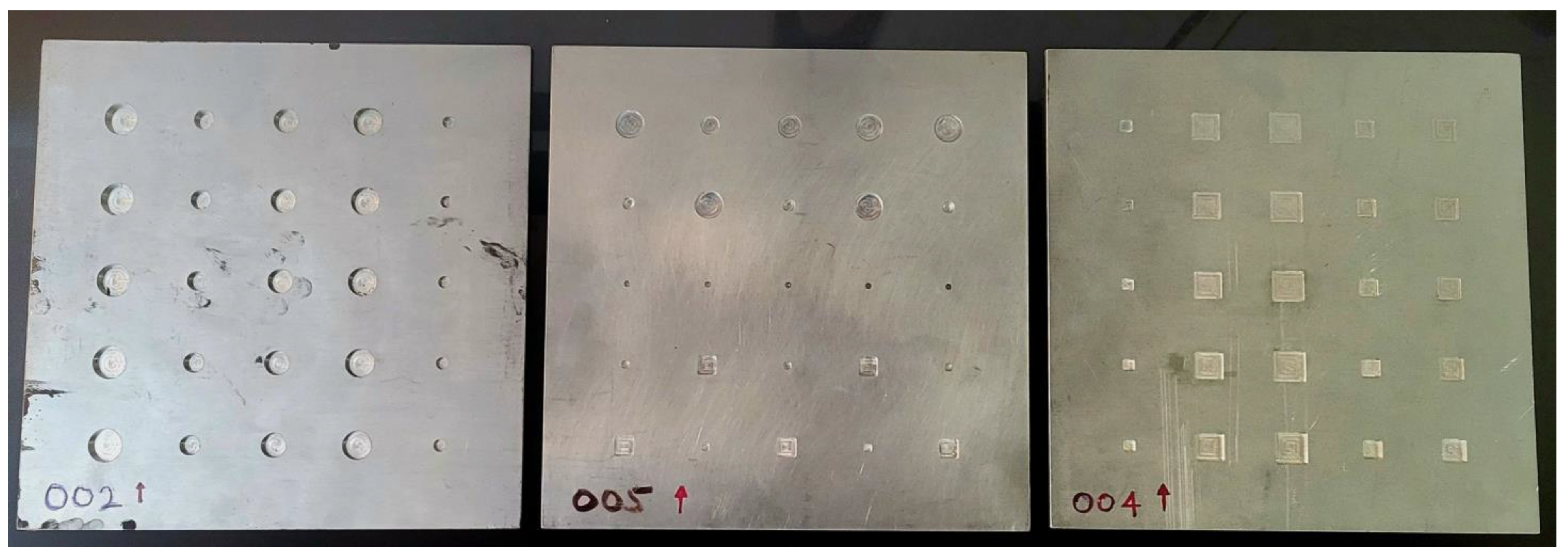
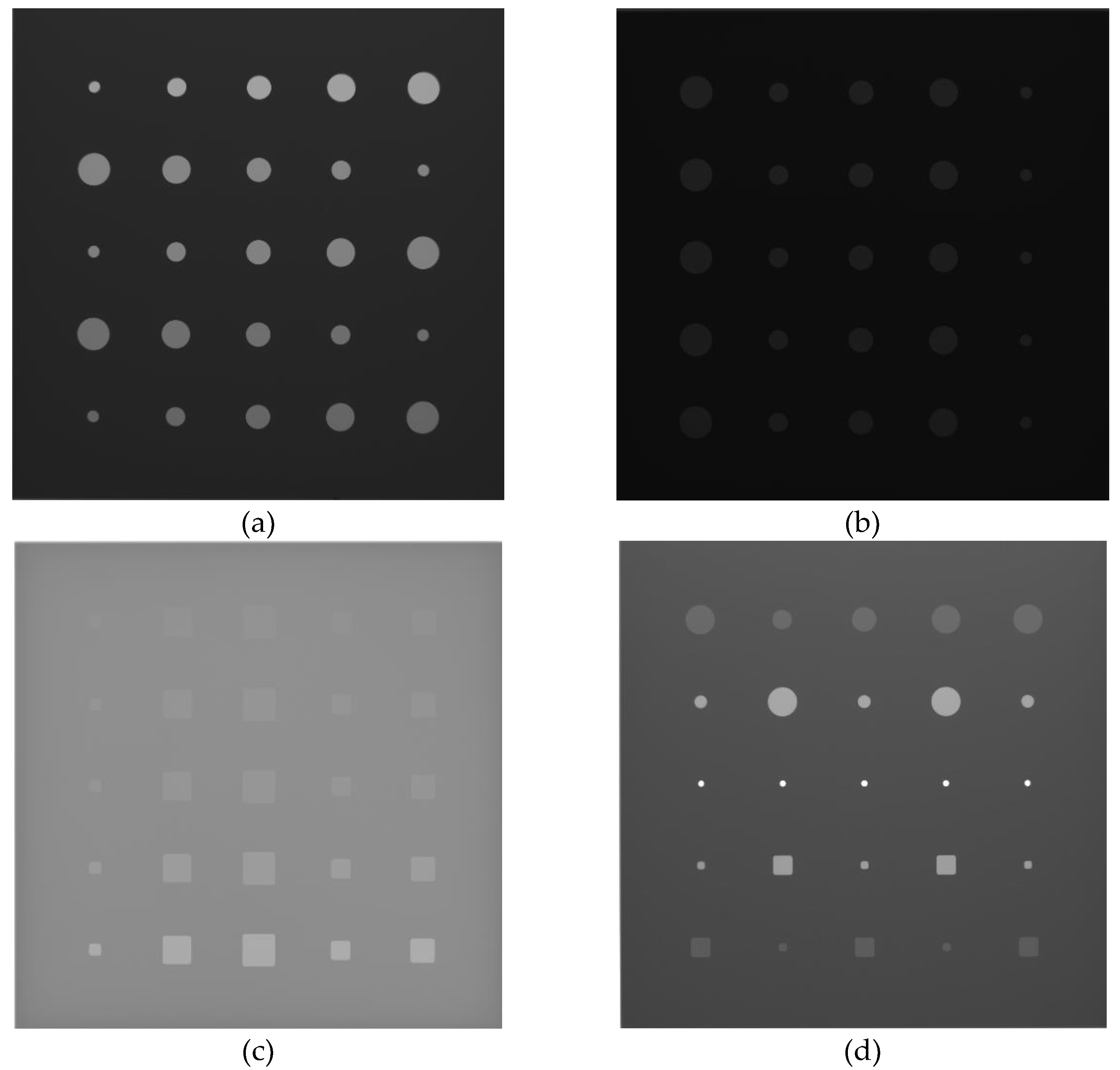
In this study, 7 square-shaped aluminum plates, each of dimensions 300mm x 300mm x 6.5mm were used for data acquisition. Each plate has 25 flat-bottom holes (totaling 175 for the entire 7 plates), with either circular or square shapes, and having depths ranging from 0.5mm (shallowest) to 5.5mm (deepest). See
Figure 1.
3.2. Data acquisition
A digital X-ray radiography imaging system with a maximum tube voltage of 150kV and maximum current of 0.5mA is used in this study. The detector is a scintillation-based 2D digital detector array DDA with 3098 x 3097 pixels. For the entire image acquisitions of the 7 plates, a fixed SDD of 600 mm, with the plates placed directly on the detector, is maintained. This is to ensure that for a particular exposure factor used, consistency is maintained in gray value distribution across all plates, at regions with the same thickness. For the flat-bottom holes with varying depths, the gray values vary, forming features that can be visually appreciated on radiographs. As shown in
Table 1., twenty distinct exposure parameters were used on each plate, while maintaining same positioning, throughout the sequence of 20 exposures. This would facilitate easier annotation of features to use as ground truth for deep learning model training.
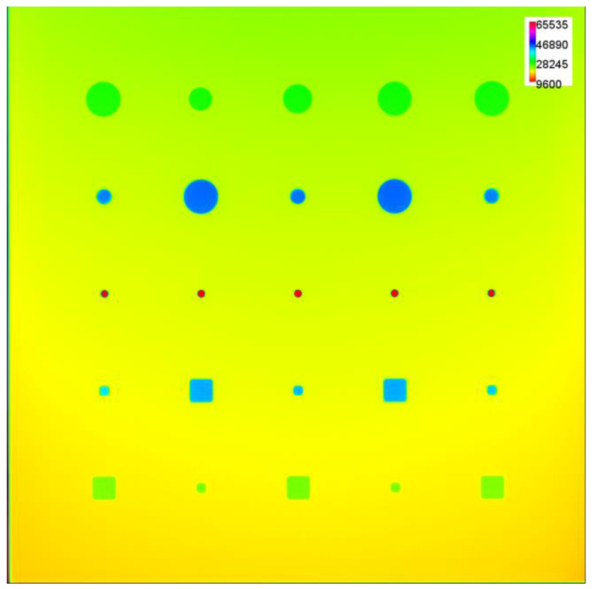
Given the DDA’s large size, a single image acquisition is sufficient to cover a 300mm x 300mm plate, however, the diverging nature of X-ray beam as it travels from the focal spot of the X-ray tube to the detector, results in an uneven distribution of X-ray intensity across the length and breadth of the detector. Another factor known as the anode heel effect also contributes to nonuniformity in X-ray beam intensity, due to the angled nature of anode target of the X-ray tube, which results in the generation of X-rays with higher intensity at the cathode side, compared to the anode side of the X-ray tube [
45]. For better visualization of these effects, the gray value distribution of an acquired image is converted to a color spectrum as shown in
Figure 2.
Due to the unevenness in GV distribution discussed above and observed in
Figure 2., SNR measurements across the pates show varying values, even at regions that are of the same thickness but located at different regions. Even though the unevenness was improved by flat-fielding technique using ISee! Software [
46], the variation in grey values is still noticeable in the images. The exposure factors and SNR measurements across a plate within each exposure category are listed in
Table 1:
3.2.1. Cropping and Dataset Preparation
To counter the problem posed by uneven distribution of GV which inadvertently affects the SNR across regions of the plates, we cropped each radiographic image into 512 x 512-pixel regions of interest (ROIs), each containing one flat-bottom hole. Therefore, from a single image, 25 cropped images were obtained, yielding a total of 3,500 images, considering 25 x 20 x 7 (feature per plate x number of exposures x number of plates).
3.2.2. Data Cleaning and Selection
Given the differing depths of the flat-bottom holes, regions with holes of higher depth attained detector saturation at high exposure factors, resulting in a pixel value of 65535 (see
Figure 2.). As these images could potentially have a negative impact on model training, we identified and excluded them from the dataset. With this technique, a total of 2,726 candidate images without any saturated pixels was realized.
3.2.3. Data sorting
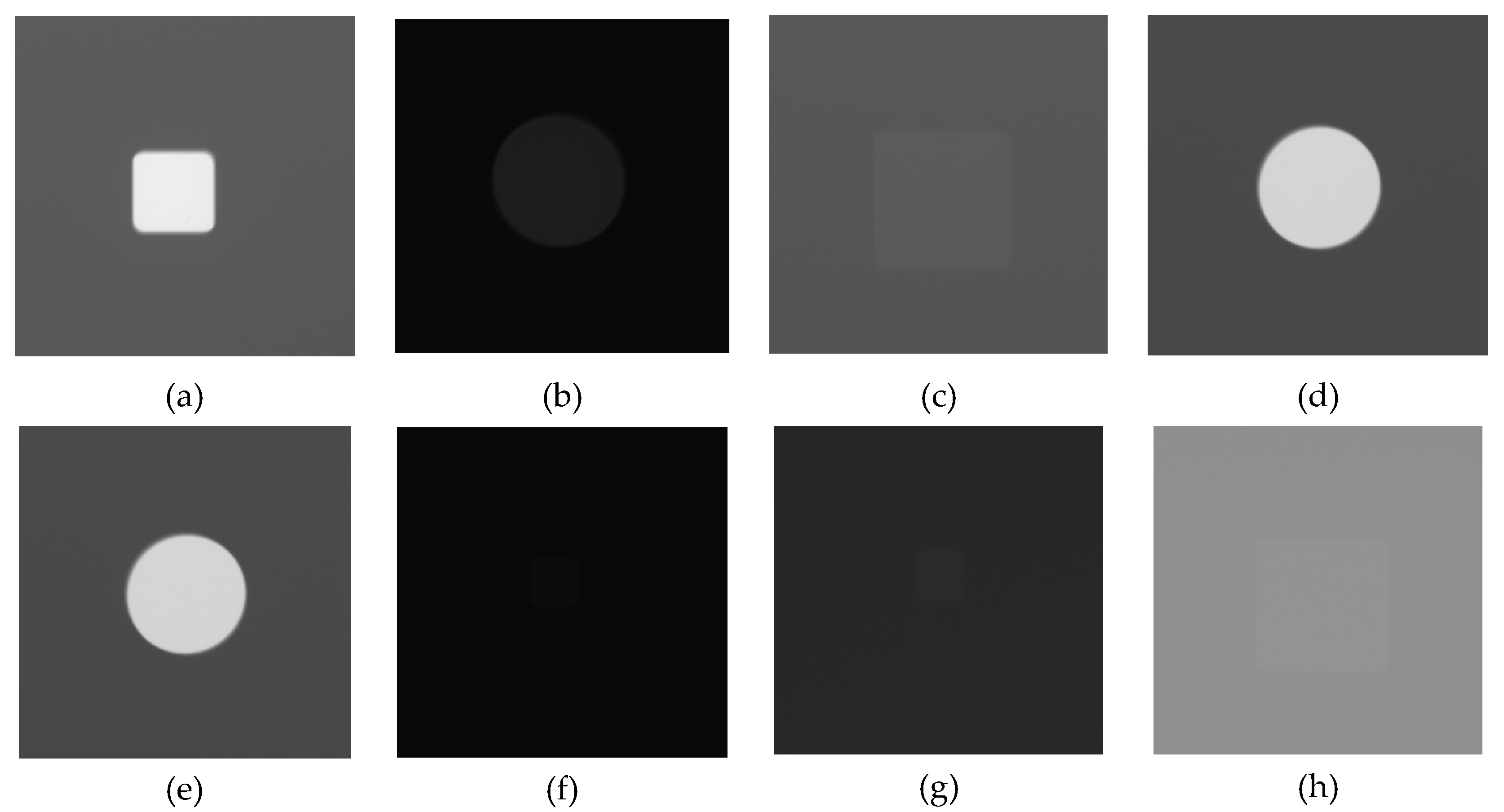
To achieve the objective of this study, the dataset containing 2,726 cleaned images was duplicated. The first dataset was realized by sorting the images based on increasing SNR measurement values. This took no account of the CNR values between the features in each image and its background. Additionally, the second dataset was sorted in order of increasing CNR values between the feature in each image and its associated background. Like the approach with sorting using SNR, this CNR sorting operation had no consideration for the SNR values.
Signal-to-Noise Ratio (SNR) is the ratio of mean value of the linearized grey values to the standard deviation of the linearized grey values (noise) in each region of interest in a digital image. The NDT Standard recommends that the region of interest shall contain at least 1,100 pixels. The SNR values are realized in accordance with equation (2). This measurement was carried out for all the 512 x 512 cleaned images, for splitting into groups in order of increasing SNR values, with each having a specific range, e.g., 0-50, 51-100, 101-150…etc.
where
μsignal is the mean of the signal and
σnoise is the standard deviation of the noise.
A copy of the dataset was sorted according to Contrast-to-Noise Ratio (CNR) values. According to EN ISO 17636-2:2022 [
47], CNR is the ratio of the difference of the mean signal levels between two ROIs to the averaged standard deviation of the signal levels. Hence, to realize this for each image in the dataset, a strategy of defining two ROIs (one on flat-bottom hole and the other on the background) was developed, considering the varying sizes of the features. Iterating this operation on all the images, CNR values were obtained according to equation (3), and the dataset was categorized into different groupings, based on the realized CNR values:
Mean pixel values of the feature and background ROIs, respectively are denoted by μ₁ and μ₂, while the standard deviation of the pixel values of the feature and background ROIs are given represented by σ₁ and σ₂ respectively.
Figure 4.
512 x 512 cropped images, with different image quality.
Figure 4.
512 x 512 cropped images, with different image quality.
3.2.4. Data Splitting and Ground Truth Generation
To adequately explore the effect of CNR and SNR on the training of flaw detection algorithms for NDT radiography images, the previously sorted images have been classified into four distinct datasets according to their CNR and SNR values. For both datasets categorized based on CNR and SNR measurements, a spectrum of values was established and designated as High or Low for each group (CNR and SNR), as can be seen in
Table 2. For the four datasets realized from this, the training, validation and
test1 data belonged to either a high or low measurement value range of CNR or SNR. Furthermore, for each of the 4 groups a second test data (
test2) was realized from images that did not fall within the range of their measurement values. This is to assess the impact of lacking such specific range of measured values (CNR or SNR) of test
2 in the training data set. For each group, dataset splitting was 60%, 20%, 20% for training, validation, and
test1, respectively.
The features on the plates were manually annotated using CVAT [
48] to generate the ground truth data for model training.
3.3. Deep Learning Model Training
This study employs the use of a U-net deep learning architecture that was initially designed for biomedical image segmentation tasks [
49]. Since its inception, U-net deep learning architecture has garnered significant interest in the field of research and is being utilized across different domains for semantic segmentation tasks [
50,
51,
52,
53,
54].
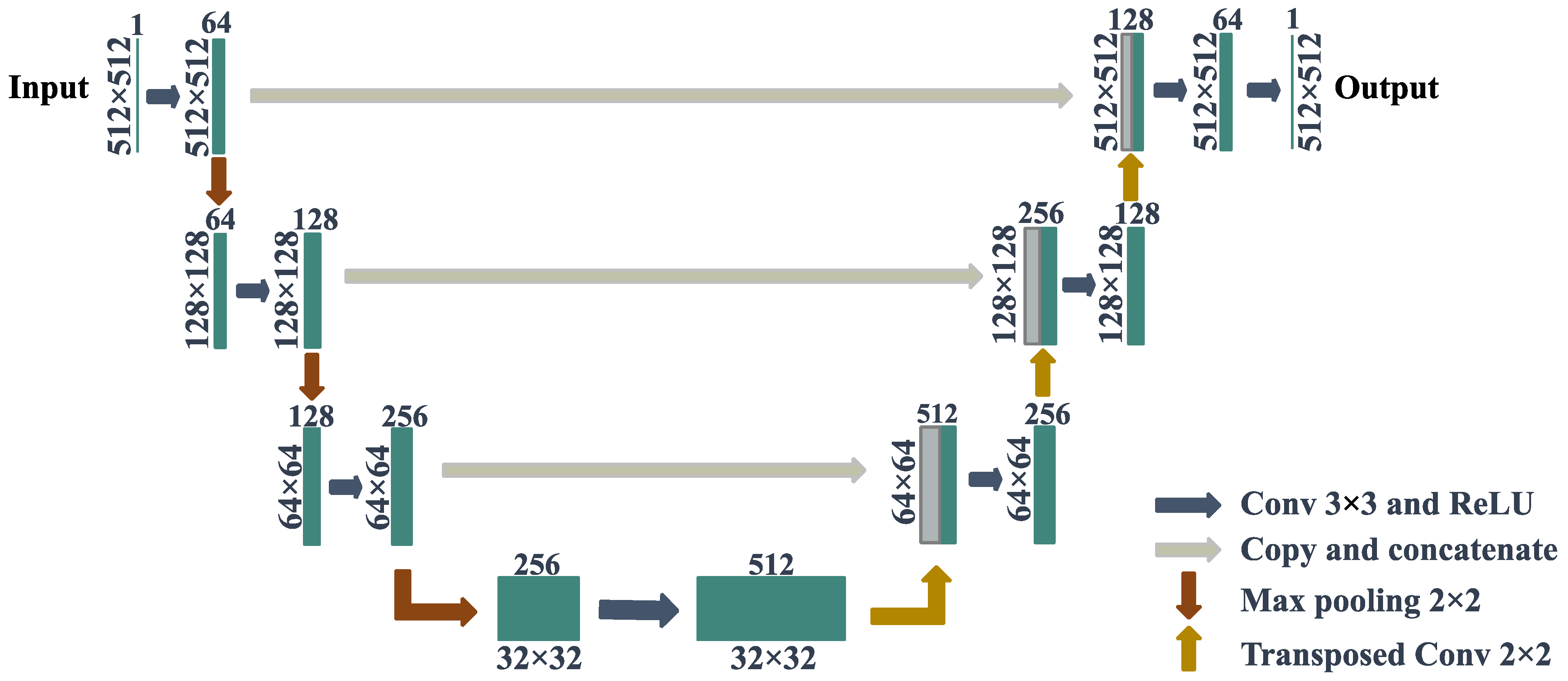
The graphical representation of the architecture of U-net can be seen in
Figure 5. The architecture comprises of an encoder-decoder structure, with skip connections that enables the recovery of high-resolution features, allowing for better precision in outcomes of segmentation tasks.
In the process of training our model, several key parameters were utilized to achieve optimal performance. The dimensions of the input images are 512 x 512 pixels, and to improve on the diversity of our dataset, we employed data augmentation techniques, including random rotation and flipping, to improve generalization. The choice of these geometric augmentation is to maintain the quality of the images, as other augmentation techniques such as elastic deformation could affect the image quality parameters (CNR and SNR) being investigated. The learning rate was set to 1e-4, and the model was trained for a total of 50 epochs. Adam optimizer was selected to update the model's weights, and binary cross-entropy loss function was utilized to measure the discrepancy between the predicted output and the ground truth.
4. Results
The results of model performance on the four datasets described in
Table 2. are presented in the
Table 3 below. For each of the 4 datasets (High SNR, Low SNR, High CNR and Low CNR), mean IoU values are displayed for their respective two test sets (
test1 and
test2)
In an interesting observation, the mean IoUs on the test images (test1 and test2) for the High SNR dataset were not significantly different. However, the mean IoU value of test1 belonging to the same category as the training datasets was slightly lower. When trained on Low SNR datasets, a comparable model performance is observed, with the mean IoUs also having slight variations. Although in this case, the test1 dataset belonging to the same range of SNR values as the training dataset reveals a slightly better model performance.
For the High CNR and Low CNR datasets, the differences in mean IoU are comparatively higher on respective test datasets (
test1 and test2) as shown in
Table 3. Like observed with the Low SNR results, the High SNR result reveals a better performance on
test1 relative to
test2. Model training with Low CNR reveals the most significant margin between its
test1 and test2 datasets, with
test1 yielding lower model performance than
test2, despite being in the same range of CNR values as the Low CNR training dataset.
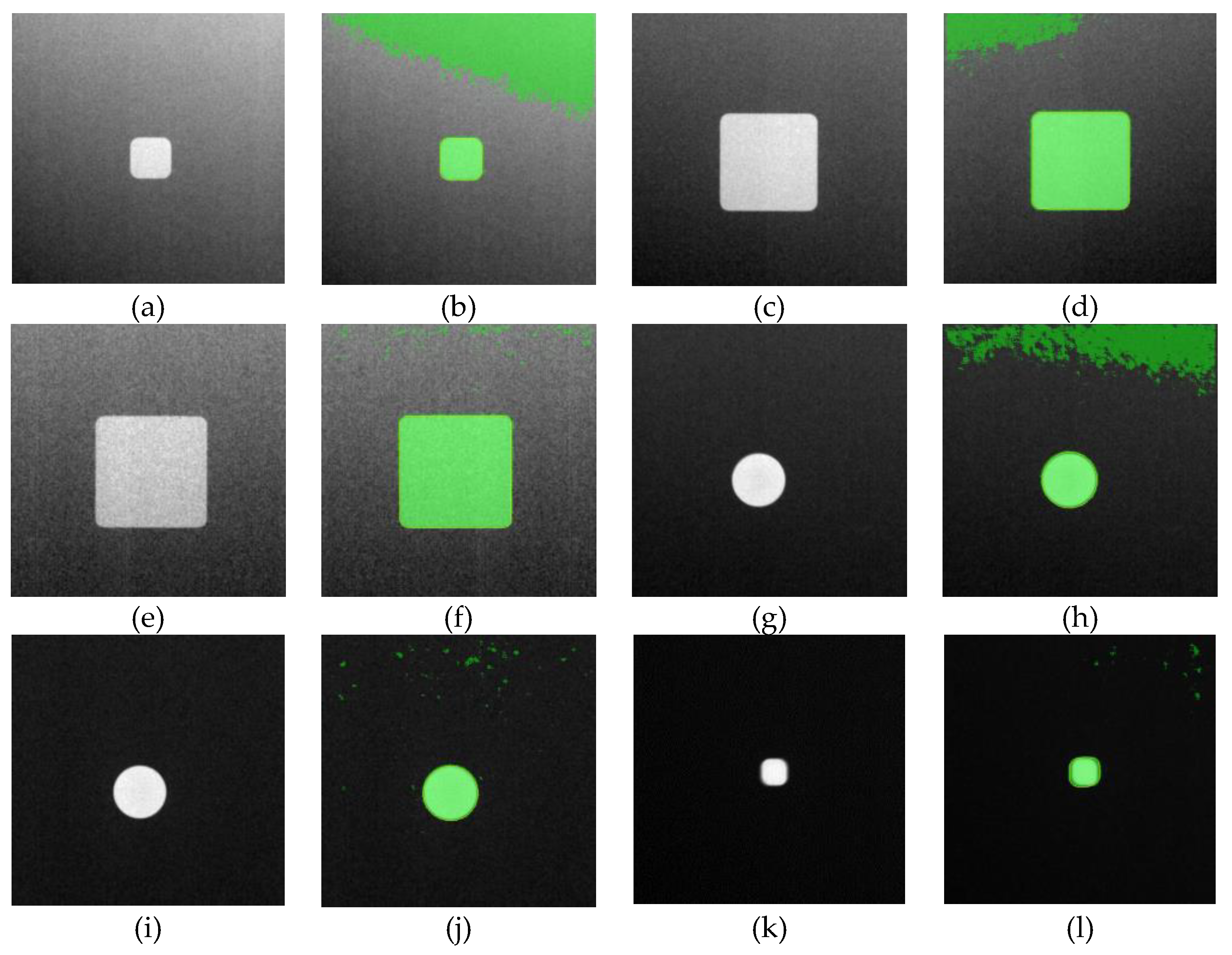
These findings, especially with the CNR datasets, led to a second run of model training using a different dataset named High CNR2, which is sorted as done previously. However, the second dataset has a narrower range of high CNR measurement values for training, validation, and test1; whereas dataset for test2, also has a narrower range of low CNR measurement values. This dropped the number of original images used for training.
The U-net model was trained on the new High CNR
2, while maintaining the same training parameters earlier mentioned. The results as seen in
Table 5. below reveals a substantial difference for CNR readings.
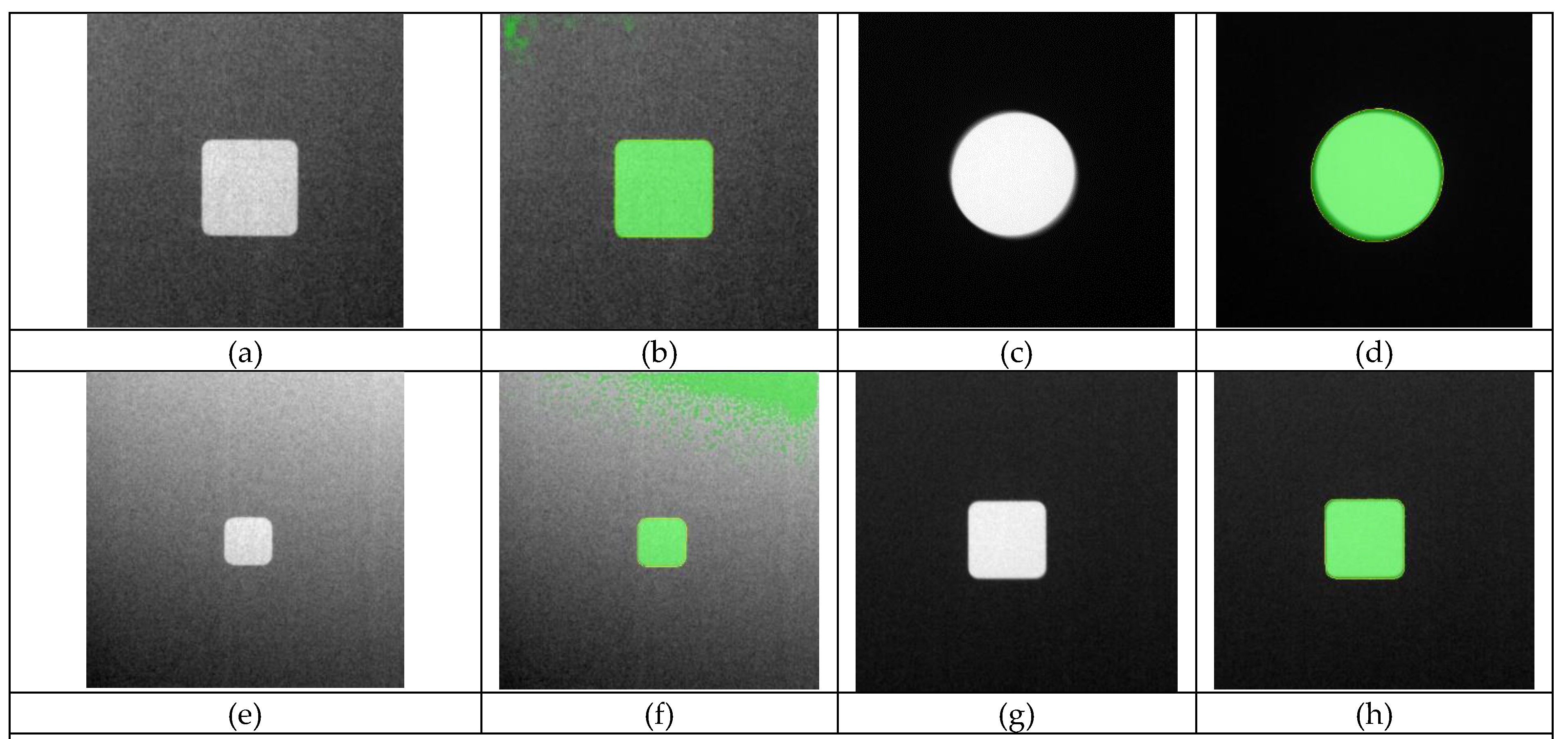
Figure 7.
Pairs of input images and semantic segmentation results, showing model performance on the training with High CNR2 dataset. (a - l) shows results from test2, images.
Figure 7.
Pairs of input images and semantic segmentation results, showing model performance on the training with High CNR2 dataset. (a - l) shows results from test2, images.
5. Discussion
Contrast-to-noise ratio (CNR) and Signal-to-noise ratio (SNR) are both associated with the signal and noise properties of radiographic image, although they have distinct meanings. While CNR represents the pixel intensity differences that exist between two regions of interest, SNR addresses the overall signal quality. Hence, there is no linearized relationship between SNR and CNR readings throughout the datasets. A decrease in CNR value could be observed in certain high SNR images, especially when the high SNR was attained by significantly increasing the energy of the X-rays (kV) during image acquisition, leading to a reduction in the differential attenuation of X-rays between regions of different thicknesses. Therefore, sorting the data according to SNR values may inadvertently lead to a stochastic distribution of CNR values (high, mid, and low) within such dataset. The same applies to sorting according to CNR values, where distribution of SNR values is random across the CNR-sorted dataset.
Model training on SNR datasets shows a comparable performance when tested on the respective test1 (belonging to the same SNR range as training data), and test2 (belonging to the opposite end of the measured SNR range dataset). We therefore posit that this improved performance could be a function of the diverse distribution of images with wider range of measured CNR values across the entire SNR-sorted datasets.
The subsequent findings on model performance with the High CNR2 dataset validates the hypothesis, where it is observed that training with datasets of limited range of measured CNR values (at the high spectrum) performs poorly (mean IoU of 0.5875) when tested on images belonging to a limited range of low CNR values. Same trained model performed well (mean IoU of 0.9594) with test images belonging to the same range of high CNR values.
6. Conclusions
The findings of this experimental study shows that image quality of digital radiography images could affect the performance of deep learning semantic segmentation model. Contrast-to-noise ratio (CNR) emerges as a most critical image quality, when compared to signal-to-noise ratio (SNR) because it focuses on specific features on the digital X-ray radiography image. SNR remains a very important image quality parameter that is used to assess the quality of an image. According to NDT Standards, SNR determines what testing class an acquired NDT X-ray radiographic image belongs to, making NDT inspectors aim to achieve such specific range of SNR quality. Nevertheless, it has been revealed in this study that having a robust representation of flaw types at different CNR values could improve the generalization of a deep learning model and reduce the chances of missing flaws during deployment. Therefore, when curating a dataset for training deep learning semantic segmentation models for digital X-ray radiography applications, an informed varying of the exposure conditions as applied in this study, could yield varied representation of flaws in terms of their CNR characteristics and potentially lead to a better generalization of the model.
Author Contributions
“Conceptualization, B.H.; methodology, B.H.; software, Z.W.; validation, B.H. and Z.W.; formal analysis, B.H. and Z.W.; investigation, B.H.; data curation, B.H.; writing—original draft preparation, B.H.; writing—review and editing, C.I.; supervision, C.I and X.M.; funding acquisition, X.M. All authors have read and agreed to the published version of the manuscript.
Funding
The authors wish to acknowledge the support of the Natural Sciences and Engineering Council of Canada (NSERC), CREATE-oN DuTy! Program (funding reference number 496439-2017), the Mitacs Acceleration program (funding reference FR49395), the Canada Research Chair in Multi-polar Infrared Vision (MIVIM), and the Canada Foundation for Innovation.
Data Availability Statement
Data could be provided upon request through the corresponding author.
Acknowledgments
We thankfully acknowledge the support and assistance provided by Mr. Luc Perron of Lynx Inspection Inc., Quebec City, Canada.
Conflicts of Interest
The authors declare no conflict of interest.
References
- Hassani, S.; Dackermann, U. A Systematic Review of Advanced Sensor Technologies for Non-Destructive Testing and Structural Health Monitoring. Sensors 2023, 23, 2204. [Google Scholar] [CrossRef] [PubMed]
- Standard Terminology for Nondestructive Examinations Available online:. Available online: https://www.astm.org/e1316-22a.html (accessed on 27 March 2023).
- Maleki, H.R.; Abazadeh, B.; Arao, Y.; Kubouchi, M. Selection of an Appropriate Non-Destructive Testing Method for Evaluating Drilling-Induced Delamination in Natural Fiber Composites. NDT & E International 2022, 126, 102567. [Google Scholar] [CrossRef]
- Gupta, M.; Khan, M.A.; Butola, R.; Singari, R.M. Advances in Applications of Non-Destructive Testing (NDT): A Review. Advances in Materials and Processing Technologies 2022, 8, 2286–2307. [Google Scholar] [CrossRef]
- Department of Pharmaceutical Quality Assurance, Pioneer Pharmacy Degree College, Sayajipura, Vadodara-390019, Gujarat, India; Patel, R. A Review on Non-Destructive Testing (NDT) Techniques: Advances, Researches and Applicability. ijcsrr 2022, 05. [CrossRef]
- ISO 9712:2021(En), Non-Destructive Testing — Qualification and Certification of NDT Personnel Available online:. Available online: https://www.iso.org/obp/ui/fr/#iso:std:iso:9712:ed-5:v1:en (accessed on 27 March 2023).
- Recommended Practice, No. SNT-TC-1A Available online:. Available online: https://asnt.org/MajorSiteSections/Standards/ASNT_Standards/SNT-TC-1A.aspx (accessed on 27 March 2023).
- Basu, S. Manufacturing and Factory Automation. In Plant Intelligent Automation and Digital Transformation; Elsevier, 2023; pp. 243–272 ISBN 978-0-323-90246-5.
- Ikumapayi, O.M.; Afolalu, S.A.; Ogedengbe, T.S.; Kazeem, R.A.; Akinlabi, E.T. Human-Robot Co-Working Improvement via Revolutionary Automation and Robotic Technologies – An Overview. Procedia Computer Science 2023, 217, 1345–1353. [Google Scholar] [CrossRef]
- Patrício, L.; Ávila, P.; Varela, L.; Cruz-Cunha, M.M.; Ferreira, L.P.; Bastos, J.; Castro, H.; Silva, J. Literature Review of Decision Models for the Sustainable Implementation of Robotic Process Automation. Procedia Computer Science 2023, 219, 870–878. [Google Scholar] [CrossRef]
- Filippi, E.; Bannò, M.; Trento, S. Automation Technologies and Their Impact on Employment: A Review, Synthesis and Future Research Agenda. Technological Forecasting and Social Change 2023, 191, 122448. [Google Scholar] [CrossRef]
- Bertovic, M. Human Factors in Non-Destructive Testing (NDT): Risks and Challenges of Mechanised NDT. 2015. [CrossRef]
- Hashem, J.A.; Pryor, M.; Landsberger, S.; Hunter, J.; Janecky, D.R. Automating High-Precision X-Ray and Neutron Imaging Applications With Robotics. IEEE Transactions on Automation Science and Engineering 2018, 15, 663–674. [Google Scholar] [CrossRef]
- García Pérez, A.; Gómez Silva, M.J.; de la Escalera Hueso, A. Automated Defect Recognition of Castings Defects Using Neural Networks. J Nondestruct Eval 2022, 41, 11. [Google Scholar] [CrossRef]
- Gao, Y.; Li, X.; Wang, X.V.; Wang, L.; Gao, L. A Review on Recent Advances in Vision-Based Defect Recognition towards Industrial Intelligence. Journal of Manufacturing Systems 2022, 62, 753–766. [Google Scholar] [CrossRef]
- Basu, S. Manufacturing and Factory Automation. In Plant Intelligent Automation and Digital Transformation; Elsevier, 2023; pp. 243–272 ISBN 978-0-323-90246-5.
- Zhao, J.D. Robotic Non-Destructive Testing of Manmade Structures: A Review of the Literature.
- Yang, L.; Fan, J.; Huo, B.; Li, E.; Liu, Y. A Nondestructive Automatic Defect Detection Method with Pixelwise Segmentation. Knowledge-Based Systems 2022, 242, 108338. [Google Scholar] [CrossRef]
- Malarvel, M.; Singh, H. An Autonomous Technique for Weld Defects Detection and Classification Using Multi-Class Support Vector Machine in X-Radiography Image. Optik 2021, 231, 166342. [Google Scholar] [CrossRef]
- Boaretto, N.; Centeno, T.M. Automated Detection of Welding Defects in Pipelines from Radiographic Images DWDI. NDT & E International 2017, 86, 7–13. [Google Scholar] [CrossRef]
- Parlak, İ.E.; Emel, E. Deep Learning-Based Detection of Aluminum Casting Defects and Their Types. Engineering Applications of Artificial Intelligence 2023, 118, 105636. [Google Scholar] [CrossRef]
- Li, Y.; Liu, S.; Li, C.; Zheng, Y.; Wei, C.; Liu, B.; Yang, Y. Automated Defect Detection of Insulated Gate Bipolar Transistor Based on Computed Laminography Imaging. Microelectronics Reliability 2020, 115, 113966. [Google Scholar] [CrossRef]
- Naddaf-Sh, M.-M.; Naddaf-Sh, S.; Zargarzadeh, H.; Zahiri, S.M.; Dalton, M.; Elpers, G.; Kashani, A.R. Defect Detection and Classification in Welding Using Deep Learning and Digital Radiography. In Fault Diagnosis and Prognosis Techniques for Complex Engineering Systems; Elsevier, 2021; pp. 327–352 ISBN 978-0-12-822473-1.
- Towsyfyan, H.; Biguri, A.; Boardman, R.; Blumensath, T. Successes and Challenges in Non-Destructive Testing of Aircraft Composite Structures. Chinese Journal of Aeronautics 2020, 33, 771–791. [Google Scholar] [CrossRef]
- Search Results for: “Standard Guide for the Qualification and Control of the Assisted Defect Recognition of Digital Radiographic Test Data” Available online:. Available online: https://www.astm.org/catalogsearch/result/?q=Standard+Guide+for+the+Qualification+and+Control+of+the+Assisted+Defect+Recognition+of+Digital+Radiographic+Test+Data (accessed on 27 March 2023).
- Yahaghi, E.; Movafeghi, A. Contrast Enhancement of Industrial Radiography Images by Gabor Filtering with Automatic Noise Thresholding. Russ J Nondestruct Test 2019, 55, 73–79. [Google Scholar] [CrossRef]
- ISO 19232-4:2013(En), Non-Destructive Testing — Image Quality of Radiographs — Part 4: Experimental Evaluation of Image Quality Values and Image Quality Tables Available online:. Available online: https://www.iso.org/obp/ui/#iso:std:iso:19232:-4:ed-2:v1:en (accessed on 27 March 2023).
- Saeid nezhad, N.; Ullherr, M.; Zabler, S. Quantitative Optimization of X-Ray Image Acquisition with Respect to Object Thickness and Anode Voltage—A Comparison Using Different Converter Screens. Nuclear Instruments and Methods in Physics Research Section A: Accelerators, Spectrometers, Detectors and Associated Equipment 2022, 1031, 166472. [Google Scholar] [CrossRef]
- Campillo-Rivera, G.E.; Torres-Cortes, C.O.; Vazquez-Bañuelos, J.; Garcia-Reyna, M.G.; Marquez-Mata, C.A.; Vasquez-Arteaga, M.; Vega-Carrillo, H.R. X-Ray Spectra and Gamma Factors from 70 to 120 KV X-Ray Tube Voltages. Radiation Physics and Chemistry 2021, 184, 109437. [Google Scholar] [CrossRef]
- Kwong, J.C.; Palomo, J.M.; Landers, M.A.; Figueroa, A.; Hans, M.G. Image Quality Produced by Different Cone-Beam Computed Tomography Settings. American Journal of Orthodontics and Dentofacial Orthopedics 2008, 133, 317–327. [Google Scholar] [CrossRef]
- Astolfo, A.; Buchanan, I.; Partridge, T.; Kallon, G.K.; Hagen, C.K.; Munro, P.R.T.; Endrizzi, M.; Bate, D.; Olivo, A. The Effect of a Variable Focal Spot Size on the Contrast Channels Retrieved in Edge-Illumination X-Ray Phase Contrast Imaging. Sci Rep 2022, 12, 3354. [Google Scholar] [CrossRef]
- Waite, S.; Farooq, Z.; Grigorian, A.; Sistrom, C.; Kolla, S.; Mancuso, A.; Martinez-Conde, S.; Alexander, R.G.; Kantor, A.; Macknik, S.L. A Review of Perceptual Expertise in Radiology-How It Develops, How We Can Test It, and Why Humans Still Matter in the Era of Artificial Intelligence. Academic Radiology 2020, 27, 26–38. [Google Scholar] [CrossRef] [PubMed]
- Standard Practice for Design, Manufacture and Material Grouping Classification of Wire Image Quality Indicators (IQI) Used for Radiology Available online:. Available online: https://www.astm.org/e0747-18.html (accessed on 28 March 2023).
- Ewert, U.; Zscherpel, U.; Vogel, J.; Zhang, F.; Long, N.X.; Nguyen, T.P. Visibility of Image Quality Indicators (IQI) by Human Observers in Digital Radiography in Dependence on Measured MTFs and Noise Power Spectra.
- Sy, E.; Samboju, V.; Mukhdomi, T. X-Ray Image Production Procedures. In StatPearls; StatPearls Publishing: Treasure Island (FL), 2023. [Google Scholar]
- Tonnessen, B.H.; Pounds, L. Radiation Physics. Journal of Vascular Surgery 2011, 53, 6S–8S. [Google Scholar] [CrossRef] [PubMed]
- Day, F.H.; Taylor, L.S. Absorption of X-Rays in Air.
- Liu, J.; Kim, J.H. A Novel Sub-Pixel-Shift-Based High-Resolution X-Ray Flat Panel Detector. Coatings 2022, 12, 921. [Google Scholar] [CrossRef]
- Markötter, H.; Müller, B.R.; Kupsch, A.; Evsevleev, S.; Arlt, T.; Ulbricht, A.; Dayani, S.; Bruno, G. A Review of X-Ray Imaging at the BAM Line (BESSY II). Adv Eng Mater 2023, 2201034. [Google Scholar] [CrossRef]
- Yang, F.; Zhang, D.; Zhang, H.; Huang, K. Cupping Artifacts Correction for Polychromatic X-Ray Cone-Beam Computed Tomography Based on Projection Compensation and Hardening Behavior. Biomedical Signal Processing and Control 2020, 57, 101823. [Google Scholar] [CrossRef]
- Dewi, P.S.; Ratini, N.N.; Trisnawati, N.L.P. Effect of X-Ray Tube Voltage Variation to Value of Contrast to Noise Ratio (CNR) on Computed Tomography (CT) Scan at RSUD Bali Mandara. ijpse 2022, 6, 82–90. [Google Scholar] [CrossRef]
- Listiaji, P.; Dewi, N.R.; Taufiq, M.; Akhlis, I.; Bayu, K.; Kholidah, A. Radiation Exposure Factors Optimization of X-Ray Digital Radiography for Watermarked Art Pottery Inspection. J. Phys.: Conf. Ser. 2020, 1567, 022008. [Google Scholar] [CrossRef]
- Utami, A.P.; Istiqomah, A.N. The Influence of X-Ray Tube Current-Time Variations Toward Signal to Noise Ratio (SNR) in Digital Radiography: A Phantom Study. Applied Mechanics and Materials 2023, 913, 121–129. [Google Scholar] [CrossRef]
- Moreira, E.; Barbosa Rabello, J.; Pereira, M.; Lopes, R.; Zscherpel, U. Digital Radiography Using Digital Detector Arrays Fulfills Critical Applications for Offshore Pipelines. EURASIP J. Adv. Signal Process. 2010, 2010, 894643. [Google Scholar] [CrossRef]
- Kusk, M.W.; Jensen, J.M.; Gram, E.H.; Nielsen, J.; Precht, H. Anode Heel Effect: Does It Impact Image Quality in Digital Radiography? A Systematic Literature Review. Radiography 2021, 27, 976–981. [Google Scholar] [CrossRef] [PubMed]
- Osterloh, K.; Bücherl, T.; Zscherpel, U.; Ewert, U. Image Recovery by Removing Stochastic Artefacts Identified as Local Asymmetries. J. Inst. 2012, 7, C04018–C04018. [Google Scholar] [CrossRef]
- ISO 17636-2:2022(En), Non-Destructive Testing of Welds — Radiographic Testing — Part 2: X- and Gamma-Ray Techniques with Digital Detectors Available online:. Available online: https://www.iso.org/obp/ui/#iso:std:iso:17636:-2:ed-2:v2:en (accessed on 27 March 2023).
- CVAT Available online:. Available online: https://www.cvat.ai/ (accessed on 29 March 2023).
- Ronneberger, O.; Fischer, P.; Brox, T. U-Net: Convolutional Networks for Biomedical Image Segmentation 2015.
- John, D.; Zhang, C. An Attention-Based U-Net for Detecting Deforestation within Satellite Sensor Imagery. International Journal of Applied Earth Observation and Geoinformation 2022, 107, 102685. [Google Scholar] [CrossRef]
- Tokime, R.B.; Maldague, X.; Perron, L. Automatic Defect Detection for X-Ray Inspection: A U-Net Approach for Defect Segmentation.
- Oztekin, F.; Katar, O.; Sadak, F.; Aydogan, M.; Yildirim, T.T.; Plawiak, P.; Yildirim, O.; Talo, M.; Karabatak, M. Automatic Semantic Segmentation for Dental Restorations in Panoramic Radiography Images Using U-Net Model. Int J Imaging Syst Tech 2022, 32, 1990–2001. [Google Scholar] [CrossRef]
- Yin, X.-X.; Sun, L.; Fu, Y.; Lu, R.; Zhang, Y. U-Net-Based Medical Image Segmentation. Journal of Healthcare Engineering 2022, 2022, 1–16. [Google Scholar] [CrossRef]
- Wei, Z.; Osman, A.; Valeske, B.; Maldague, X. Pulsed Thermography Dataset for Training Deep Learning Models. Applied Sciences 2023, 13, 2901. [Google Scholar] [CrossRef]
|
Disclaimer/Publisher’s Note: The statements, opinions and data contained in all publications are solely those of the individual author(s) and contributor(s) and not of MDPI and/or the editor(s). MDPI and/or the editor(s) disclaim responsibility for any injury to people or property resulting from any ideas, methods, instructions or products referred to in the content. |
© 2023 by the authors. Licensee MDPI, Basel, Switzerland. This article is an open access article distributed under the terms and conditions of the Creative Commons Attribution (CC BY) license (http://creativecommons.org/licenses/by/4.0/).
