1. Introduction
is a major air pollutant that can significantly impact human health, including respiratory and cardiovascular diseases [
1]. Therefore, accurate and detailed information on
concentrations is essential for assessing and managing the impacts of air pollution.
In recent years, advances in remote sensing and satellite data have enabled high-resolution
concentration maps at regional and global scales [
2,
3]. These maps can provide valuable information to policymakers, researchers, and the general public. They help to plan and evaluate efforts to improve air quality and protect human health. However, due to inherent remote sensing limitations, they remain a temporal snapshot (or a mosaic of snapshots), sometimes misinterpreted as monthly or annual average concentrations. Still, the demand for high-resolution concentration maps needs additional means [
4].
Using mathematical equations, air quality models can simulate the transport and dispersion of
particles in the atmosphere. These models use meteorological data, emission inventories, and other inputs to estimate
concentrations at high spatial and temporal resolution. This method can generate
concentration maps from regional to global scales. While air quality models can be accurate, they require significant computational resources and depend on the quality of input data. There are several classes of air quality models[
5], including CTM (Chemical Transport Models), which are based on mass and momentum conservation equations and are the most universal and general. Since pollutant transport is highly linked to meteorological conditions, CTMs are often run together with meteorological models (online approach) or demand the results of a meteorological model (offline approach).
Gaussian plume models are analytical and widely used due to their low computational demands [
6]. These models provide an analytical solution to the pollutant transport equation, assuming one of the atmosphere stability classes. They are usually applied for a single stack to assess its environmental impact [
7].
Another rapidly emerging approach for obtaining air quality concentration maps is the application of machine learning techniques (also known as data-driven modelling) [
8]. In this case, the user is only responsible for defining the input data set (like meteorological parameters, land use, and emission inventory data) and target variables (usually concentrations). These models act as black-box models, trained using supervised learning processes. Depending on the output type - they can be classified as classification or regression models. The most popular ones include neural networks (focusing on LSTM networks [
9]), random forests [
10] or spatial kriging algorithms [
11].
Data fusion methods can combine data from different sources [
12], such as ground-based monitoring, satellite remote sensing, and air quality models, to generate high-resolution
concentration maps. These methods use statistical and machine learning techniques to merge the data and estimate
concentrations at locations where data are missing or incomplete. While data fusion methods can improve the accuracy and spatial resolution of
concentration maps, benefiting from multiple approaches, they must be applied cautiously as they often produce non-physical results [
13,
14].
This paper uses Random Forest to describe and evaluate a data fusion technique from two sources (the regional GEM-AQ model[
15] and the local Gaussian plume model). We discuss several approaches to using random forests in a diverse area of southern Poland. The proposed approach was tested on a regional domain, routinely modelled with a coarse-resolution regional model. The proposed approach can also act as a form of air quality model results downscaling. This region was chosen due to data availability and reported air-quality issues in the past. Observation and emission data from the while year 2021 were used.
2. Data and Methods
In this study, we used the GEM-AQ model 24 h forecast from the operational run and the national air quality monitoring network observations. The study period covered the year 2021.
2.1. Study Area
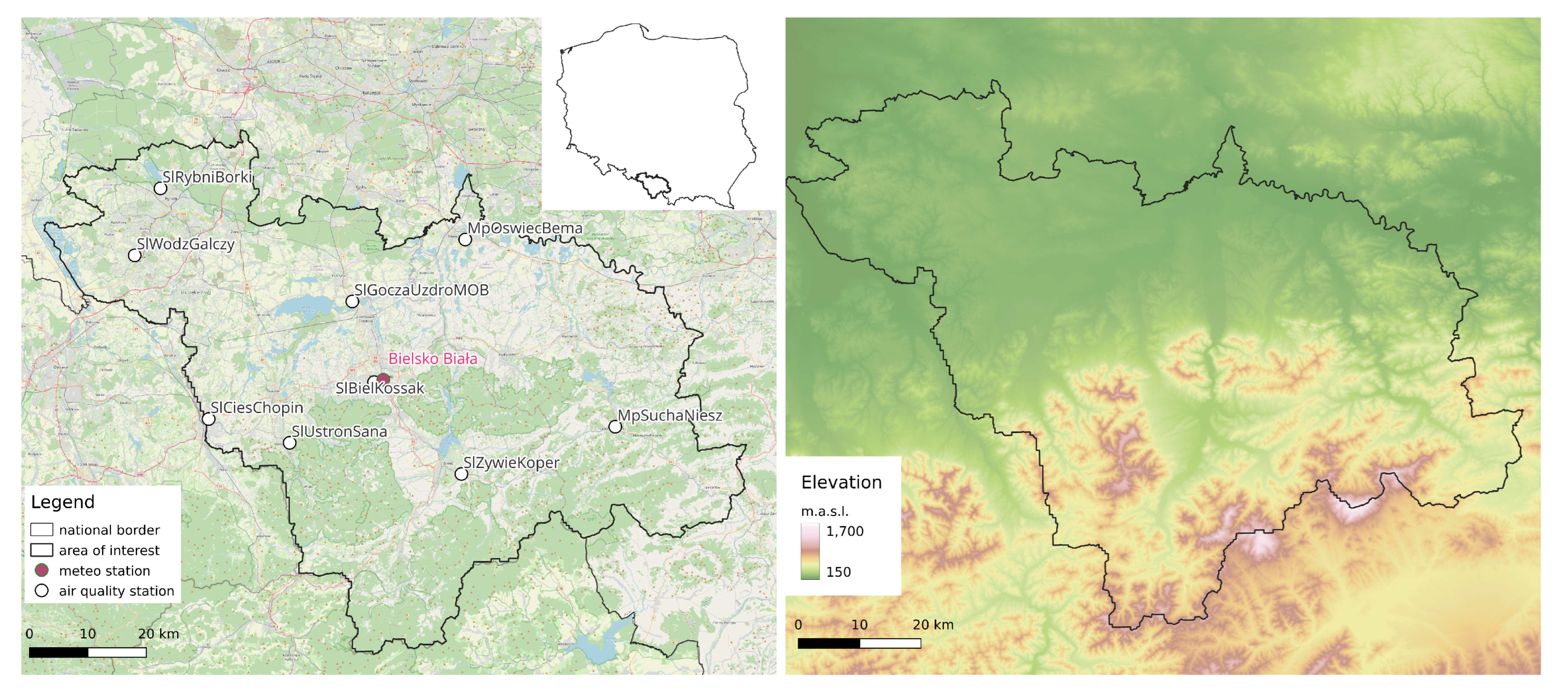
The study area is located in southern Poland, covering an area of around 5300
in Silesian and Lesser Poland voivodships (
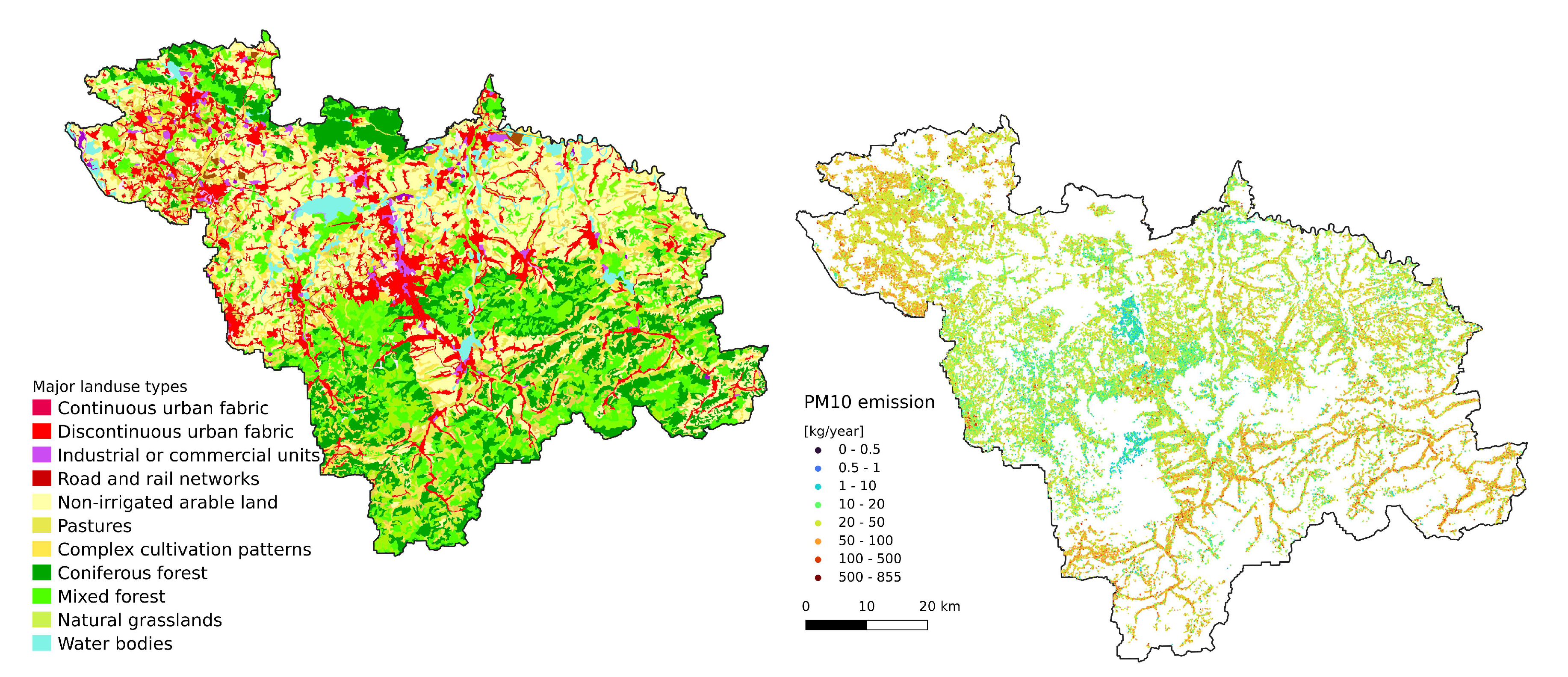
Figure 1A). The area is populated with almost 1.7 mln people. The largest cities include Bielsko Biała (170 000 inhabitants), Rybnik (140 000 inhabitants) and Jastrzębie-Zdrój (91 000 inhabitants). The northern part of the study area covers the upper Vistula valley with a high urbanization level (
Figure 2B). In contrast, the southern part reaches the Carpathian mountains, which limit air mass exchange (
Figure 1B). Temperature inversion is frequently observed, especially in foothill valleys in the winter period. This fact limits the boundary layer mixing and contributes to poor air quality [
16]. As a consequence, cities within the study area suffer from poor air quality due to high
concentration[
17]
2.2. The GEM-AQ Model
The GEM-AQ is a semi-Lagrangian chemical weather model in which air quality processes (chemistry and aerosols) and tropospheric chemistry are implemented online in the operational weather prediction model, the Global Environmental Multiscale (GEM) [
18] model, which was developed at Environment Canada. The gas-phase chemistry mechanism used in the GEM-AQ model is based on a modified version of the Acid Deposition and Oxidants Model (ADOM) [
19], where additional reaction in the free troposphere was included [
15].
The GEM-AQ model is set up to perform calculations using 28 vertical layers, out of which the lower 21 layers are classified as the troposphere.
Emission data from the polish national emission inventory drive emission sources within the model. These data are based on annual reporting obligations the facilities’ owners fulfil. Annual emissions are transformed into monthly emission rates using the weighting factor from annual emission profiles. Emission profiles are assigned to so-called SNAP categories [
20].
2.3. The Gaussian plume model
A Gaussian plume model is a widely used mathematical model for predicting the dispersion of pollutants in the atmosphere. The model assumes that the dispersion of pollutants can be approximated as a two-dimensional Gaussian distribution, which spreads out in a pattern similar to the shape of a bell curve.
The Gaussian plume model is based on the idea that a combination of atmospheric turbulence and wind patterns determines the dispersion of pollutants. The model considers factors such as the source strength and height, wind speed and direction, and atmospheric stability. The topography of the modelled area is not considered.
The Gaussian plume model is used in various applications, including air quality assessments for industrial facilities, roadway emissions, and wildfires. It is often used with other models or measurement techniques to provide a comprehensive picture of air quality in a given area.
The Gaussian plume model was implemented in a parallel Python code. The model is based on the Gaussian plume formula [
21], which describes the one-hour average concentration distribution at the surface level:
where
is the one-hour average wind velocity (assumed to be uniform over the whole computational domain),
and
are the standard deviations (horizontal and vertical) of plume concentration spatial distribution, which were estimated using formulas proposed by Briggs [
22,
23]:
Coefficients depend on the atmosphere stability class (A-F).
Atmosphere stability was classified based on gradient Richardson number criteria [
24]. The gradient Richardson number was estimated based on the meteorological output from the GEM-AQ model. The vertical gradients were calculated between the two lowest layers.
H is the plume rise above the surface, which is a sum of stack height
and plume rise
calculated using the combination of Holland and CONCAWE formulas (
,
respectively)[
25], depending on the heat flux:
2.4. Emission data
The Polish national emission inventory fully covers the study area. Three major emission SNAP categories from the inventory were used in gaussian modelling: domestic, industrial and transport emissions[
26]. Annual emissions are transformed into monthly emission rates using the weighting factor from annual emission profiles
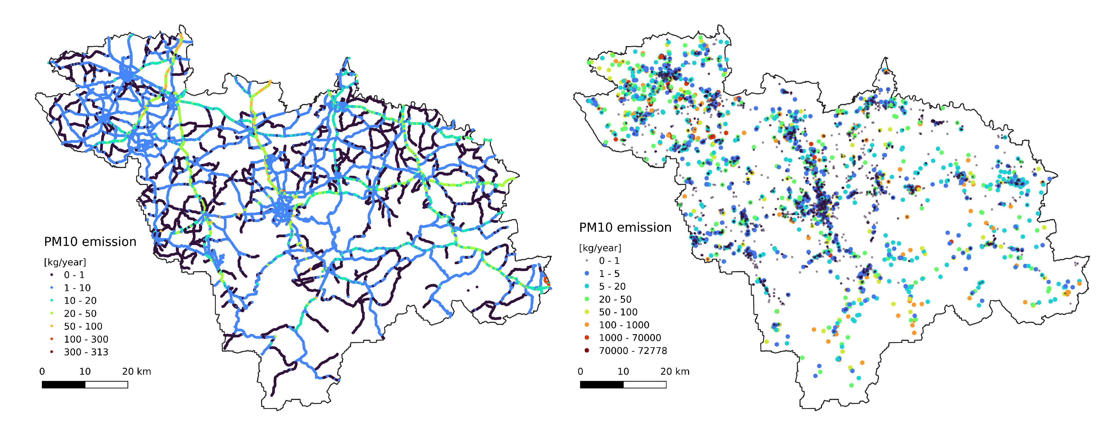
Traffic emissions were represented as point sources distributed across 30 meters along the road network (
Figure 3A). For the uplift formula (eq.
4), we assumed fumes temperature 500K and velocity
. Domestic emissions are based on the National Database of Topographic Objects (BDOT), a nationwide system of collecting and sharing topographic data, including vector data describing each building as the basis for national emission inventory[
26]. For the gaussian model, we assumed stack height as 3.5 times the number of floors + 0.5 meters. Fumes temperature was assumed to be 400K and velocity
.
Industrial emissions are based on annual reporting obligations, which the facilities’ owners fulfil to the unit responsible for managing the national emission inventory.
2.5. Surface Observations
There are nine air quality stations within the study area. Each of them measures
concentration with an hourly time step. One meteorological station is located in the centre of the area (
Figure 1).
Table 1 summarizes the annual observed air quality series. Despite the annual mean at a moderate level (30-40
), the number of days with the legal threshold (50
) exceeded is quite significant and covers the major part of the winter season.
2.6. Random forest
As a data fusion algorithm, Random Forest was used. Random Forest is a robust machine learning algorithm used for classification [
27], and regression tasks [
28]. It is a type of ensemble learning algorithm that combines multiple decision trees to improve the predictive performance of the model[
29]. Each decision tree in a random forest is constructed using a different subset of the training data and a random subset of the input features. This is done to introduce diversity and reduce overfitting, as each tree is trained on a different subset of the data and features.
In this work, we trained a random forest algorithm to predict observed concentrations at the observation station locations. Input features included concentrations from GEM-AQ and the Gaussian plume model. The models were trained using a 5-fold cross-validation process. We also attempted to use calendar-related variables such as the day of the week number and the month and observed meteorological parameters as additional features. The training dataset was based on time series observations from all nine observation stations.
As a second trial, we tried using datasets based on observations from a single observation station’s time series. This is because air quality observations are primarily influenced by each station’s location, and merging time series from multiple locations may not always be the best approach [
30].
Finally, we attempted station vs station cross-validation, as we anticipate the presence of clusters of similar stations in terms of air quality dynamics within the analyzed area. Additionally, information about outliers (i.e., stations that are different from the others) would be helpful in excluding them from the training dataset.
3. Results
3.1. Overall Performance
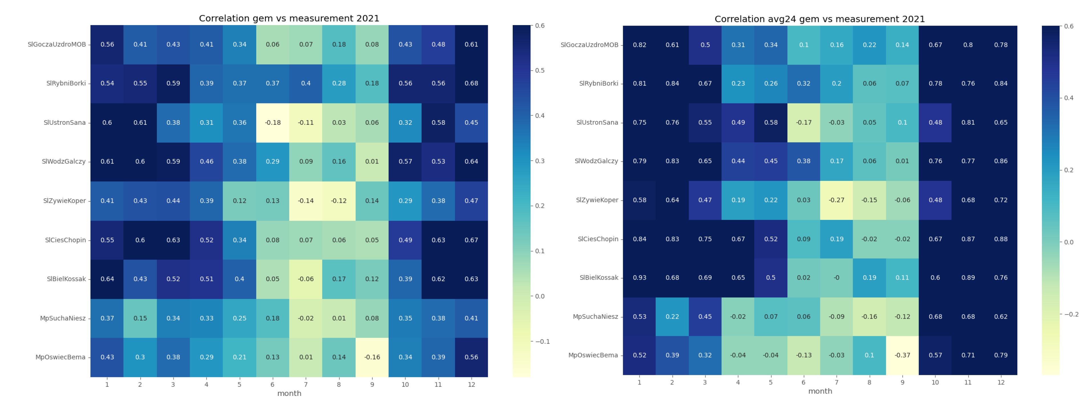
In order to assess the reproducibility of
concentration dynamics, we examined the coefficient of determination
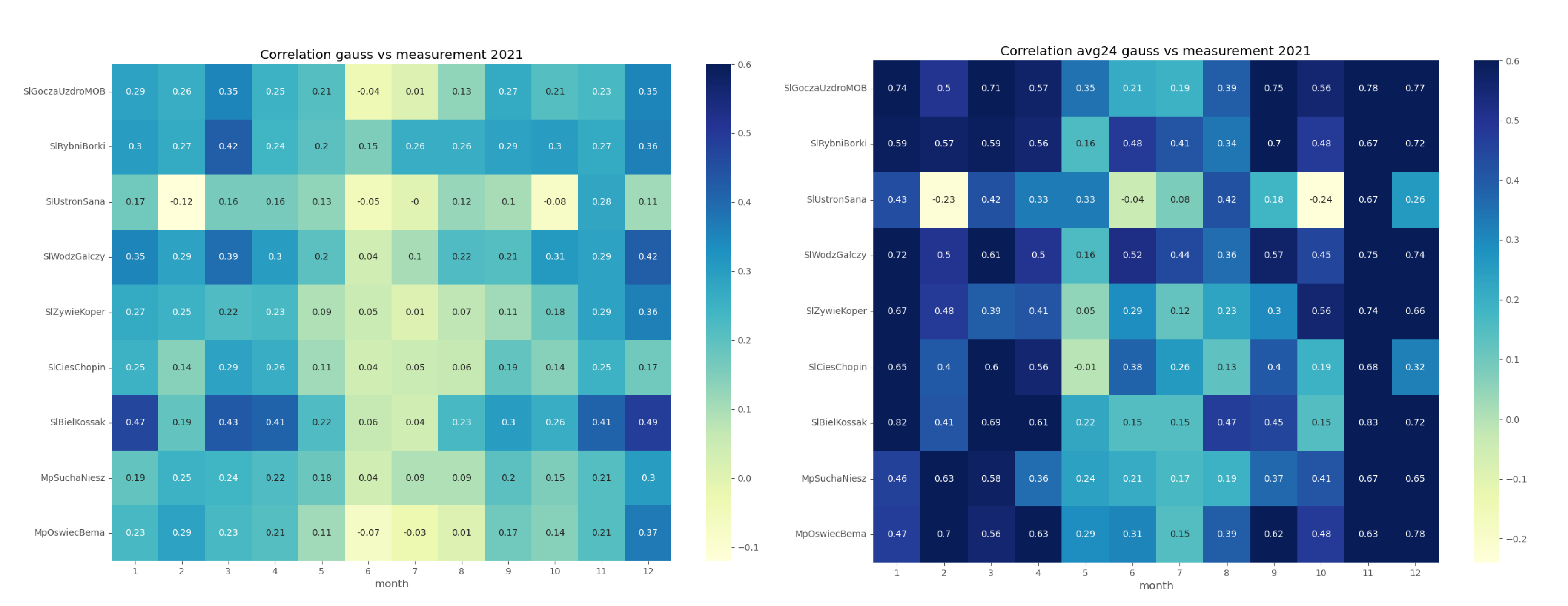
of the GEM-AQ and Gaussian plume models within a monthly time window (
Figure 4 and
Figure 5). Both models appear to perform better in winter months (October-March) than in summer (April-September). This pattern is observed at all air quality stations and can be explained by the meteorological factors driving
concentration, which are better reproduced in winter than in summer. Another reason might be the temporal emission profile, which is more uniform in winter (due to constant demand for heating) than in summer when the daily profile is not uniform.
Both GEM-AQ and Gaussian plume models perform better regarding daily averaged concentration. This fact is due to rapid changes in observed concentrations, which cannot be simulated by any of these models [
31]. Some authors [
32] explain this concentration variation by emission, which is driven by the air temperature.
Random forest performance was evaluated based on
, suitable for assessing the dynamics reproducibility. For assessing accuracy, the accuracy coefficient (
), which describes how accurate the results predicted by the random forest (
) are in comparison to observations (
y):
As the
Table 2 reveal - reproducing hourly dynamics of
concentration was challenging, regardless of the extra features. Using daily averaged concentrations instead of hourly concentration has increased the
from around 0.2 to 0.4 and accuracy from 48% to 60%. Using additional features improves model dynamics in all cases while the accuracy remains almost the same.
3.2. Temporal Comparison
We analyzed the performance of random forest models trained on data from one month only. We used 5-fold cross-validation and data from all the observation stations. The process was repeated for hourly data and daily averages. As the data from
Table 3 reveal - the best performance in terms of dynamics reproduction (
) was obtained for winter months. At the same time, the accuracy (thus reproduction of the magnitude of observed concentrations) was better in the summer months. This fact can be explained by a general tendency of ensemble methods which are not very good at reproducing peak values. Also, some authors claim that a significant amount of emissions is not included in the national emission inventory [
33,
34].
3.3. Spatial Comparison
Finally, we analyzed if the choice of observation station location influenced the performance of the random forest. We used a 5-fold cross-validation process and data from one station at a time. The results make it possible to distinguish stations with sufficiently better performance (SlBielKossak, SlWodzGalczy) and stations with significantly worse one (MpSuchaNiesz, MpOswiecBema) -
Table 4. This difference can be explained when we look at the station location. The former is located in dense urban areas with local district heating systems. In contrast, the latter is located in a single-family housing area with typical low-stack residential heating emissions.
3.4. Annual statistics
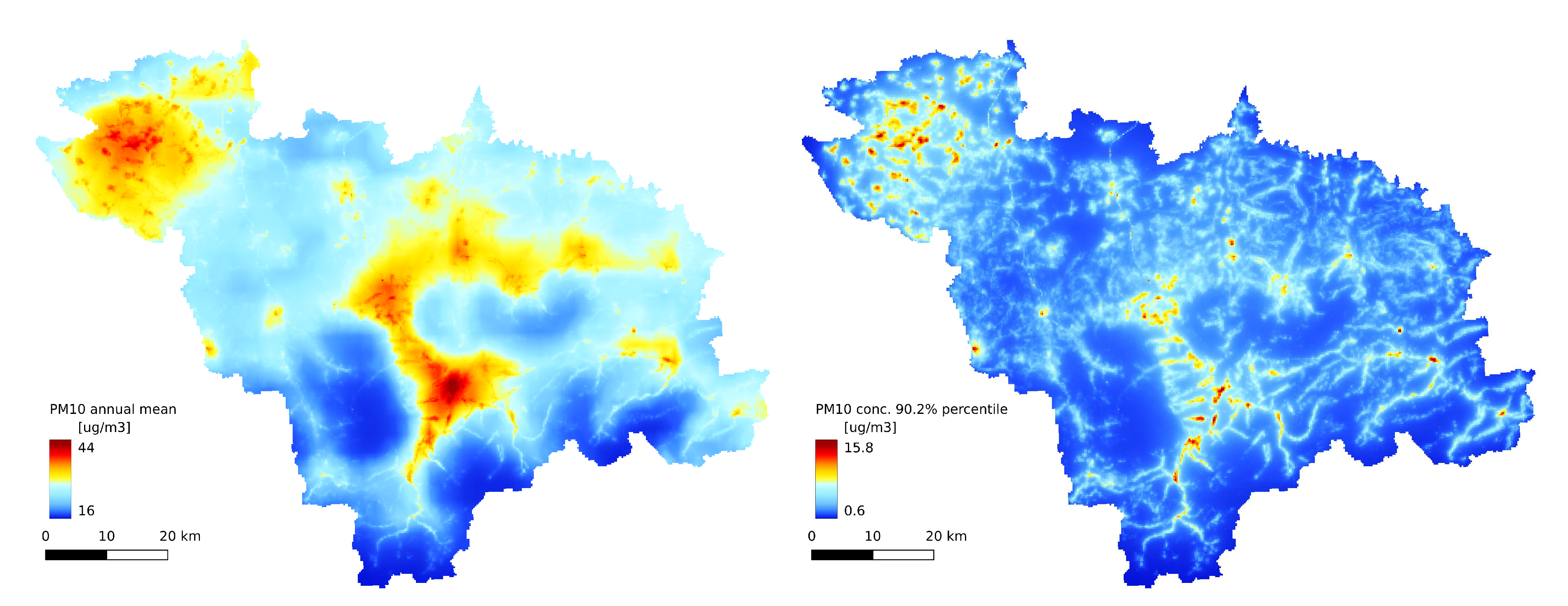
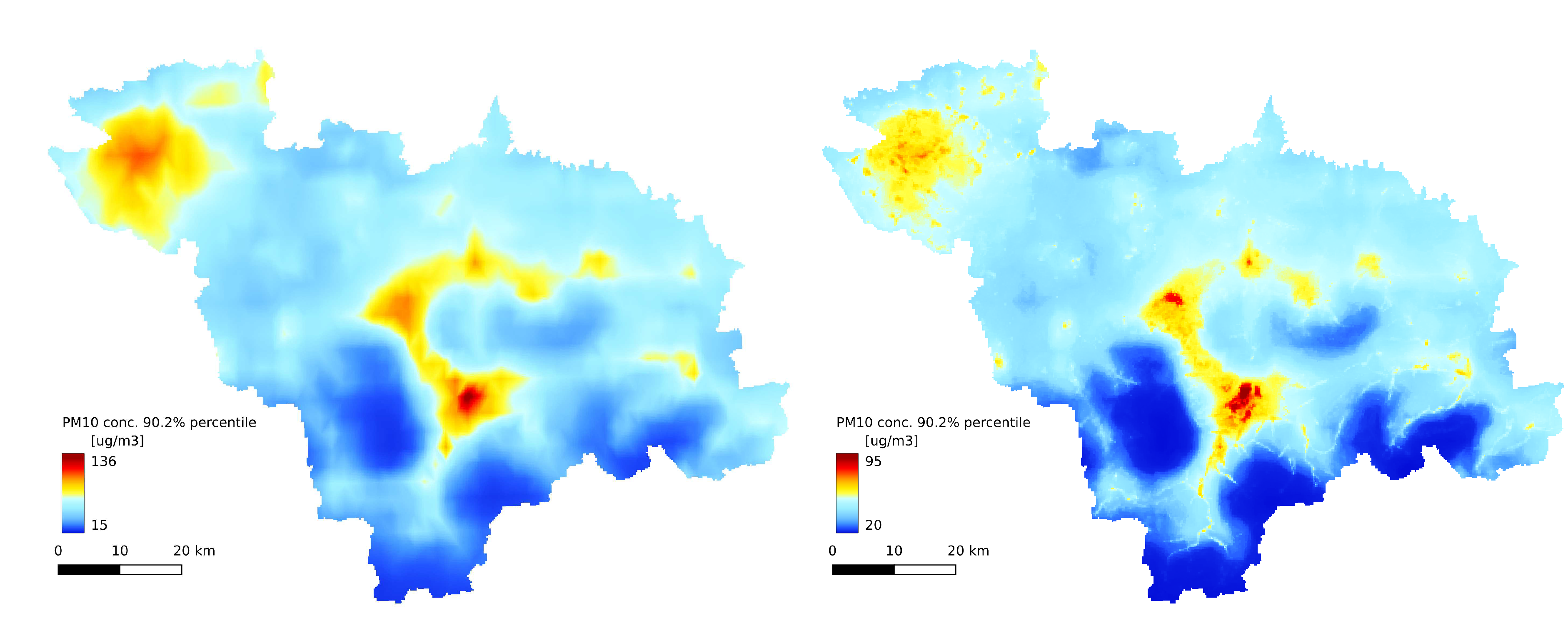
The annual statistics of the GEM-AQ model (
Figure 6A,
Figure 9A and
Figure 8A) resemble the emission pattern (
Figure 3 and
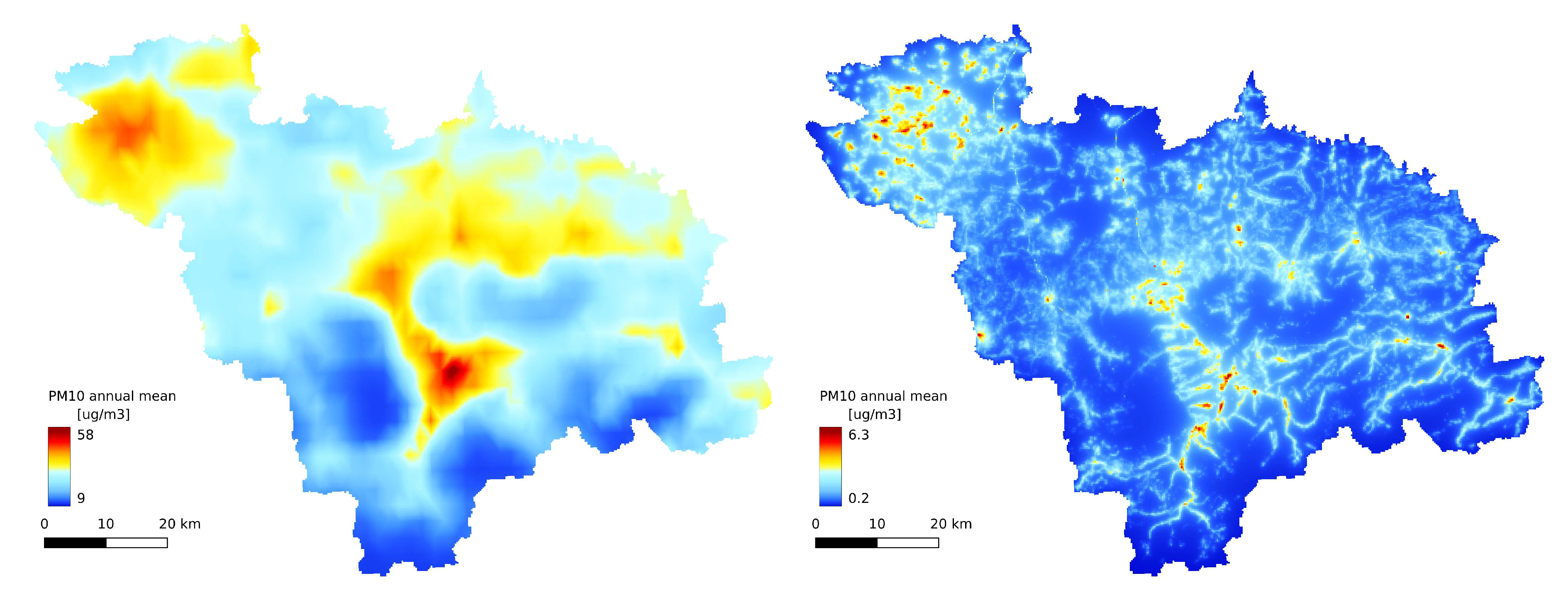
Figure 2B). High concentrations are observed in the western part of the study area (Rybnik and Wodzisław cities) and the centre (Bielsko-Biała and Żywiec). Results from the Gaussian plume model highly underestimate the average
concentration (
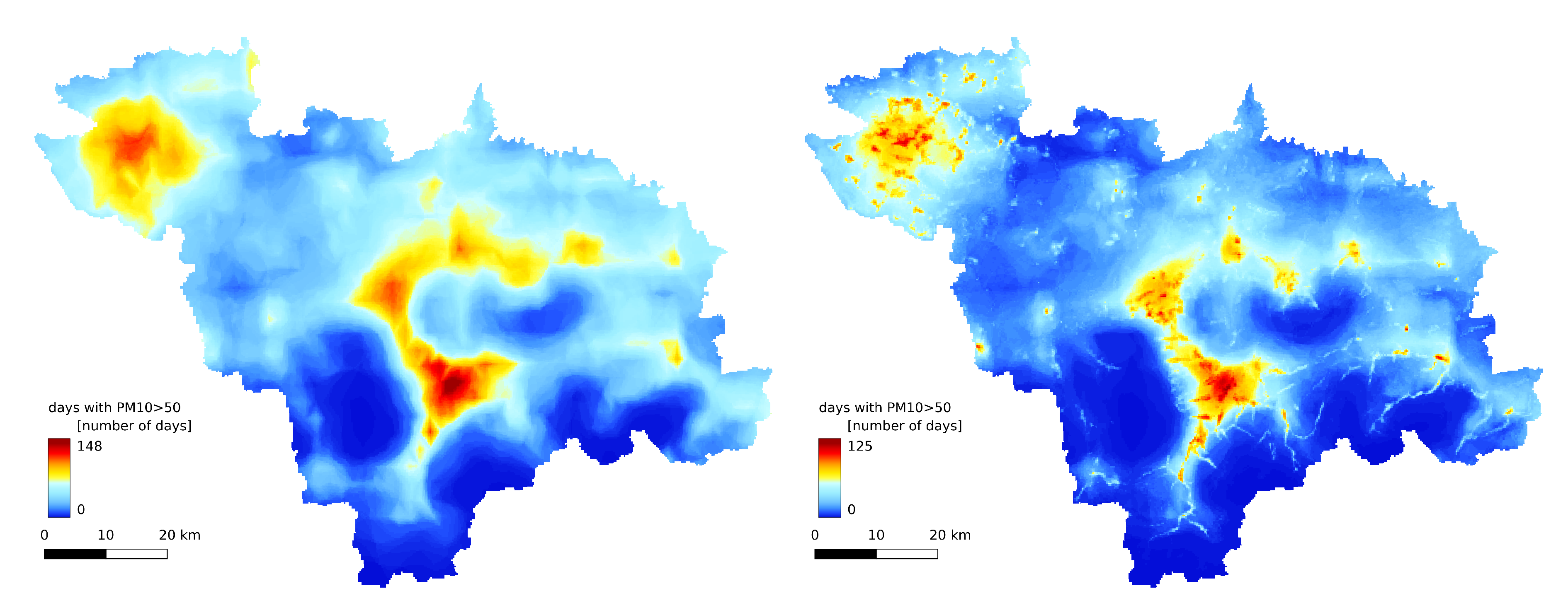
Figure 6B). Both the Gaussian plume model and random forest reveal a complex concentration pattern in the southern part of the study area, resulting from complex topography. The order of magnitude of the random forest results is similar to that of the GEM-AQ model. The random forest is not good at reproducing peak concentrations; thus, the percentile 90.2% for the random forest is generally lower than for GEM-AQ (
Figure 8). Also, the number of days when the legal threshold of
is exceeded is lower for a random forest than for GEM-AQ.
4. Conclusion
Random forest regression is a powerful and robust technique for developing non-linear regression models. As we have shown, it can be applied to obtaining high-resolution concentration maps based on regional model results. As a random forest cannot extrapolate data, its results are slightly underestimated.
The accuracy of random forest improves when applied to daily averaged values. This is likely due to the smoothing effect of averaging, thanks to which no sharp gradients must be simulated. Additional improvements to the random forest regression model can be made by using additional features. Including the day of the week and month improved both accuracy and dynamics of all random forest variants. These features act as a non-explicit temporal profile, which helps to adjust regression to emission temporal changes. Including meteorological observation (temperature and wind) as additional features, is also helpful in improving random forest regression results. However, the improvement is less significant in this case. The effect of meteorological observations is likely a way of fixing the inaccuracy of meteorological results of the GEM-AQ model, which later on affected the air quality results.
The choice of observation stations for random forest training should be made with care. Some stations tend to deliver observations which could be more challenging to replicate. On the other hand, using single observation station time series as a training target over large areas may produce results which lack universality.
Author Contributions
Conceptualization: J.S.; methodology, software, validation, resources, data curation: M.K.; writing—original draft preparation: M.K.; writing—review and editing: J.S.; visualization: M.K.; supervision: J.W.K.; project administration, J.W.K. All authors have read and agreed to the published version of the manuscript.
Funding
This research received no external funding
Institutional Review Board Statement
Not applicable
Informed Consent Statement
Not applicable.
Conflicts of Interest
The authors declare no conflict of interest.
References
- Jagiello, P.; Struzewska, J.; Jeleniewicz, G.; Kaminski, J.W. Evaluation of the Effectiveness of the National Clean Air Programme in Terms of Health Impacts from Exposure to PM2. 5 and NO2 Concentrations in Poland. International Journal of Environmental Research and Public Health 2022, 20, 530. [Google Scholar] [CrossRef]
- Emili, E.; Popp, C.; Petitta, M.; Riffler, M.; Wunderle, S.; Zebisch, M. PM10 remote sensing from geostationary SEVIRI and polar-orbiting MODIS sensors over the complex terrain of the European Alpine region. Remote sensing of environment 2010, 114, 2485–2499. [Google Scholar] [CrossRef]
- Alvarez-Mendoza, C.I.; Teodoro, A.C.; Torres, N.; Vivanco, V. Assessment of remote sensing data to model PM10 estimation in cities with a low number of air quality stations: a case of study in Quito, Ecuador. Environments 2019, 6, 85. [Google Scholar] [CrossRef]
- Park, J.; Lee, P.S.H. Relationship between Remotely Sensed Ambient PM10 and PM2. 5 and Urban Forest in Seoul, South Korea. Forests 2020, 11, 1060. [Google Scholar] [CrossRef]
- Leelossy, Á.; Molnár, F.; Izsák, F.; Havasi, Á.; Lagzi, I.; Mészáros, R. Dispersion modeling of air pollutants in the atmosphere: a review. Open Geosciences 2014, 6, 257–278. [Google Scholar] [CrossRef]
- Veigele, W.J.; Head, J.H. Derivation of the Gaussian plume model. Journal of the Air Pollution Control Association 1978, 28, 1139–1140. [Google Scholar] [CrossRef]
- Lutman, E.; Jones, S.; Hill, R.; McDonald, P.; Lambers, B. Comparison between the predictions of a Gaussian plume model and a Lagrangian particle dispersion model for annual average calculations of long-range dispersion of radionuclides. Journal of environmental radioactivity 2004, 75, 339–355. [Google Scholar] [CrossRef] [PubMed]
- Rybarczyk, Y.; Zalakeviciute, R. Machine learning approaches for outdoor air quality modelling: A systematic review. Applied Sciences 2018, 8, 2570. [Google Scholar] [CrossRef]
- Navares, R.; Aznarte, J.L. Predicting air quality with deep learning LSTM: Towards comprehensive models. Ecological Informatics 2020, 55, 101019. [Google Scholar] [CrossRef]
- Kaminska, J.A. The use of random forests in modelling short-term air pollution effects based on traffic and meteorological conditions: a case study in Wrocław. Journal of environmental management 2018, 217, 164–174. [Google Scholar] [CrossRef]
- Ignaccolo, R.; Mateu, J.; Giraldo, R. Kriging with external drift for functional data for air quality monitoring. Stochastic environmental research and risk assessment 2014, 28, 1171–1186. [Google Scholar] [CrossRef]
- Liu, J.; Li, T.; Xie, P.; Du, S.; Teng, F.; Yang, X. Urban big data fusion based on deep learning: An overview. Information Fusion 2020, 53, 123–133. [Google Scholar] [CrossRef]
- Sarigiannis, D.A.; Soulakellis, N.A.; Sifakis, N.I. Information fusion for computational assessment of air quality and health effects. Photogrammetric Engineering & Remote Sensing 2004, 70, 235–245. [Google Scholar]
- Friberg, M.D.; Kahn, R.A.; Holmes, H.A.; Chang, H.H.; Sarnat, S.E.; Tolbert, P.E.; Russell, A.G.; Mulholland, J.A. Daily ambient air pollution metrics for five cities: Evaluation of data-fusion-based estimates and uncertainties. Atmospheric Environment 2017, 158, 36–50. [Google Scholar] [CrossRef]
- Kaminski, J.; Neary, L.; Struzewska, J.; McConnell, J.; Lupu, A.; Jarosz, J.; Toyota, K.; Gong, S.; Côté, J.; Liu, X.; others. GEM-AQ, an on-line global multiscale chemical weather modelling system: model description and evaluation of gas phase chemistry processes. Atmospheric chemistry and physics 2008, 8, 3255–3281. [Google Scholar] [CrossRef]
- Liu, B.; Ma, X.; Ma, Y.; Li, H.; Jin, S.; Fan, R.; Gong, W. The relationship between atmospheric boundary layer and temperature inversion layer and their aerosol capture capabilities. Atmospheric Research 2022, 271, 106121. [Google Scholar] [CrossRef]
- Kobza, J.; Geremek, M.; Dul, L. Characteristics of air quality and sources affecting high levels of PM 10 and PM 2.5 in Poland, Upper Silesia urban area. Environmental monitoring and assessment 2018, 190, 1–13. [Google Scholar] [CrossRef]
- Côté, J.; Gravel, S.; Méthot, A.; Patoine, A.; Roch, M.; Staniforth, A. The operational CMC–MRB global environmental multiscale (GEM) model. Part I: Design considerations and formulation. Monthly Weather Review 1998, 126, 1373–1395. [Google Scholar] [CrossRef]
- Venkatram, A.; Karamchandani, P.; Misra, P. Testing a comprehensive acid deposition model. Atmospheric Environment (1967) 1988, 22, 737–747. [Google Scholar] [CrossRef]
- Tagaris, E.; Sotiropoulou, R.E.P.; Gounaris, N.; Andronopoulos, S.; Vlachogiannis, D. Effect of the Standard Nomenclature for Air Pollution (SNAP) categories on air quality over Europe. Atmosphere 2015, 6, 1119–1128. [Google Scholar] [CrossRef]
- Stockie, J.M. The mathematics of atmospheric dispersion modeling. Siam Review 2011, 53, 349–372. [Google Scholar] [CrossRef]
- Hanna, S.R.; Briggs, G.A.; Hosker Jr, R.P. Handbook on atmospheric diffusion. Technical report, National Oceanic and Atmospheric Administration, Oak Ridge, TN (USA …, 1982.
- Davidson, G. A modified power law representation of the Pasquill-Gifford dispersion coefficients. Journal of the Air & Waste Management Association 1990, 40, 1146–1147. [Google Scholar]
- Mohan, M.; Siddiqui, T. Analysis of various schemes for the estimation of atmospheric stability classification. Atmospheric Environment 1998, 32, 3775–3781. [Google Scholar] [CrossRef]
- Carson, J.E.; Moses, H. The validity of several plume rise formulas. Journal of the air pollution control association 1969, 19, 862–866. [Google Scholar] [CrossRef]
- Gawuc, L.; Szymankiewicz, K.; Kawicka, D.; Mielczarek, E.; Marek, K.; Soliwoda, M.; Maciejewska, J. Bottom–Up Inventory of Residential Combustion Emissions in Poland for National Air Quality Modelling: Current Status and Perspectives. Atmosphere 2021, 12, 1460. [Google Scholar] [CrossRef]
- Cutler, D.R.; Edwards Jr, T.C.; Beard, K.H.; Cutler, A.; Hess, K.T.; Gibson, J.; Lawler, J.J. Random forests for classification in ecology. Ecology 2007, 88, 2783–2792. [Google Scholar] [CrossRef]
- Smith, P.F.; Ganesh, S.; Liu, P. A comparison of random forest regression and multiple linear regression for prediction in neuroscience. Journal of neuroscience methods 2013, 220, 85–91. [Google Scholar] [CrossRef]
- Breiman, L. Random forests. Machine learning 2001, 45, 5–32. [Google Scholar] [CrossRef]
- Pearce, J.L.; Beringer, J.; Nicholls, N.; Hyndman, R.J.; Tapper, N.J. Quantifying the influence of local meteorology on air quality using generalized additive models. Atmospheric Environment 2011, 45, 1328–1336. [Google Scholar] [CrossRef]
- Werner, M.; Kryza, M.; Ojrzyńska, H.; Skjøth, C.A.; WałBszek, K.; Dore, A.J. Application of WRF-Chem to forecasting PM10 concentration over Poland. International Journal of Environment and Pollution 2015, 58, 280–292. [Google Scholar] [CrossRef]
- Reizer, M.; Juda-Rezler, K. Explaining the high PM 10 concentrations observed in Polish urban areas. Air Quality, Atmosphere & Health 2016, 9, 517–531. [Google Scholar]
- Kicińska, A.; Mamak, M. Health risks associated with municipal waste combustion on the example of Laskowa commune (Southern Poland). Human and Ecological Risk Assessment: An International Journal 2017, 23, 2087–2096. [Google Scholar] [CrossRef]
- Wojdyga, K.; Chorzelski, M.; Rozycka-Wronska, E. Emission of pollutants in flue gases from Polish district heating sources. Journal of cleaner production 2014, 75, 157–165. [Google Scholar] [CrossRef]
|
Disclaimer/Publisher’s Note: The statements, opinions and data contained in all publications are solely those of the individual author(s) and contributor(s) and not of MDPI and/or the editor(s). MDPI and/or the editor(s) disclaim responsibility for any injury to people or property resulting from any ideas, methods, instructions or products referred to in the content. |
© 2023 by the authors. Licensee MDPI, Basel, Switzerland. This article is an open access article distributed under the terms and conditions of the Creative Commons Attribution (CC BY) license (http://creativecommons.org/licenses/by/4.0/).
