1. Introduction
Autonomous underwater vehicles (AUV) usually use Inertial Navigation System (INS) as the primary navigation device, but INS requires regular calibration to be able to perform long-term missions. In underwater situation, traditional navigation methods (e.g., GPS) are greatly limited due to the complexity and variability in the underwater environment[
1,
2,
3]. In contrast, the Gravity-Aided Inertial Navigation System (GAINS) is an advanced technology used for underwater navigation that enables highly accurate position estimation without emitting or receiving signals. To achieve this objective, GAINS utilizes a specially designed navigation algorithm to compare the gravimeter’s measurements of gravity anomalies at the current position with the stored gravity field data to effectively correct the INS position.[
4,
5,
6,
7]. However, the variability of the gravity field significantly affects the performance of GAINS, making the selection of suitable navigation areas crucial[
8,
9]. In this regard, researchers have explored several quantitative characteristics such as variance, roughness, slope, coefficient of variation, fractal dimension, and their combinations to determine the efficiency of using gravity fields for navigation[
10,
11,
12]. The navigation map is then divided into two categories : informative (suitable for positioning) and non-informative (not suitable for positioning) based on empirical thresholds[
13]. Informative areas are free to move around, while non-informative areas are to be avoided. And Then, intelligent optimization algorithms like genetic algorithms, simulated annealing algorithms, ant colony algorithms, and particle swarm algorithms, etc. are employed to optimize the underwater path based on the position and motion information of underwater objects[
14,
15,
16,
17,
18]. Those approaches ensure optimal obstacle avoidance and the shortest possible paths for efficient navigation.
Previous path planning algorithms for GAINS often assumed that non-informative areas were off-limits, leading to significant navigation errors. This assumption, however, may not always hold true. Unsuitable places do not necessarily equate to restricted areas, for example, a flat area unsuitable for navigation but without real obstacles. Furthermore, research suggests that areas suitable for positioning based on local characteristics are typically discrete and small, making it difficult to find connected informative areas [
13,
19,
20]. As a result, path planning using this approach is impossible in arbitrary sea areas, particularly when non-informative areas surround the start or endpoints. Therefore, the main objective of this study is to minimize the positioning error between departure and destination, rather than focusing on factors such as avoiding islands or maintaining motion control.
The performance of path planning is closely related to the navigation algorithm. Therefore, in this paper, the optimal paths will be considered by the results of the navigation filtering algorithm. The posterior Cramér-Rao bound (PCRB) integrates information from kinetics and measurement models; therefore, it comprises all sensor-obtained gravity field information without the need for actually implementing the filtering algorithm[
21,
22,
23,
24,
25,
26]. A* algorithm is one of the most common heuristic search algorithms, swiftly investigating a possible set of solutions for a given issue using heuristic search techniques, focusing more on the end answer than on sub-problems, which enables it to produce pathways fast and with improved results[
27,
28]. This study uses PCRB as the cost function of A *, precisely fusing the path planning and navigation filter estimation results. The characteristics of the gravity fields at departure and destination are not limitations on the proposed path-planning method. This study doesn’t add distance directly to the cost or heuristic function like most shortest path trajectory designs do. Instead, the distance factor is included in the INS error divergence variance. Hence, this method can plan the quickest path while maintaining positioning accuracy.
The following arrangement of this paper is as follows. Section II derives the PCRB model of GAINS, and Section III combines PCRB with A* to form the PCRB-based A* path planning method. In Section IV, two simulation tests are done to see if the two planned paths are the best ones. Finally, conclusions are given in Section V.
2. PCRB for Gravity-Aided Navigation System
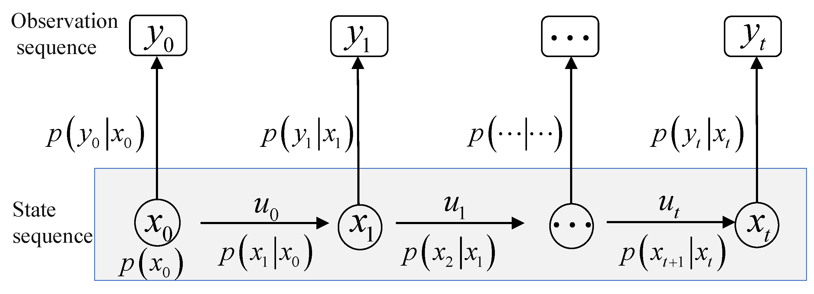
In most cases, GAINS is modeled as a hidden Markov model (HMM), as shown in
Figure 1, i.e., the observation depends only on the state of the Markov chain at that moment, independent of the other states; the current moment state is related only to the previous moment.
The mathematical model of GAINS can be reduced to the following two discrete-time equations.The first equation describes the evolution of the state vector, i.e., the INS error propagation process
where
is the state vector indicating the carrier position.
represents the state increment of INS.
represents the state noise from IMU measurement error, Gaussian distribution, and with covariance matrix
.
The second equation describes the observed values of the gravity sensor and the comparison with the reference map values by interpolation
where
is the measurement of the gravimeter at time
t, and
h denotes the interpolation method of the gravity sensors model combined with the reference data map, usually sampling bilinear or Kriging interpolation.
denotes the measurement noise of the geophysical sensor, which is assumed to be additive Gaussian white noise.
denotes the reference data mapping error. Considering this error covariance depending on the location, the variance matrix of the total observation error modeled as (
3) [
29].
where
includes a combination of sensor measurements and map uncertainty.
is the map spatial resolution,
is the map mapping error variance.
is the variance of the local gravity anomaly.
is the inverse of the square of the correlation distance, and
is the gravimeter measurement error variance.
Under the assumption of additive Gaussian white noise,
and
, are assumed to be independent of each other, and independent of
. (
1), (
2) explicitly determine the joint probability distribution
of
and
at any moment
t with a known
.
where
refers to the probability density of the variables described in the parameters of
p. The derivation of (
4) makes use of the Markov property of the model i.e.
, and
.
PCRB is a lower bound on the mean squared error (MSE) of a deterministic parameter estimate in parameter estimation, defined as the variance of any unbiased estimate being at least larger than the inverse of the Fisher information. Whenever the estimate
is based on the sequence
, the mean square error for any unbiased estimator
should satisfy the following condition.
where
is the Fisher information matrix.
where
denotes the joint probability density of
and
. Here and below,
∇ is the operator of the first order derivative, and
is the operator of the second order derivative.
Let
denote the PCRB of the state
determined for a given measurement
. By decomposing the lower bound (
5) into subblocks, the estimated covariance of
is lower bounded by the lower right block of
, i.e.
Insert (
4) into (
8) to get the recursive update
where
denotes the block matrix of zero entries of appropriate dimensionality.
Comparing with (
9), it follows that
Under the assumption that the noise
and
of (
1) and (
2) are zero-mean Gaussian and invertible covariance matrices,
and
, respectively, therefore
where
and
are constants. Thus, in the equation (
11),
where
and
is the gradient of
at the true position at time
t. In the above derivation, the expectation of both the measurement noise and the position is 0, so the expectation
is computed only at the current true position.
Bringing the equation (
14)-() into the equation (
11) gives
The derivation of (
17) makes use of the Woodbury matrix identity[
30].
in (
17) is only related to the position and represents the gravitational positioning information obtained from the map, and the square root of the trace of this matrix is used as the scalar navigation information map.
A further expansion of equation (
17) using the Woodbury matrix identity gives a more interesting form
(
20) and () constitute the recursive form of the PCRB for the state estimation in GAINS, where (
20) is the one-step prediction covariance and () is the posterior filter covariance. The recursively estimated PCRB is consistent with the error covariance Riccati recursion of the Kalman filter to the system by linearizing the model around the true state sequence.
This also indicates that the Kalman filter can obtain the optimal solution under the assumption of linear Gaussian white noise, and its state covariance can reach the PCRB.
3. A* Algorithm Path Planning Design Based on PCRB
The A* algorithm is a heuristic search algorithm that is recursive in nature and can follow certain steps, starting from the original state and gradually searching to the optimal solution. The A* algorithm uses the overhead G between nodes in the graph, and a heuristic function H related to the current task to find the optimal path.
Where, is the valuation function of a node, which indicates the combined priority of that node considered in the selection of node n. denotes the actual generation value from the starting point to the current node. denotes the cost estimate of the current node to the target point, which is the prediction function.
The computation in PCRB is in the time domain and the A* algorithm works in the spatial domain. To facilitate the combination of PCRB with the A* algorithm, the coordinates at
t time are assumed to be
n. Correspondingly, the estimated position PCRB in
n coordinates is
. The INS position error dispersion is assumed to be time-dependent only, and the coefficient of linear drift of the position error variance with time is
. Denote the Euclidean distance from the current point
to the parent node
by
, and denote the distance from the current point to the target node by
to denote the Euclidean distance from the current point to the target node.
The position error uncertainty of INS grows linearly over a certain time period, and the relationship between
and distance is as follows.
where
is the average velocity of the carrier during the sampling interval.
The main goal of this paper is to identify the path that minimizes the total posterior filtering errors of navigation at each current waypoint. We accomplish this by using the PCRB
at the present position
n as the cost function
for the current node in the A algorithm.
(
26) represents the navigation error covariance of the one-step prediction, and () represents the correction of the one-step prediction by the posterior information from the reweighted force measurement to obtain the PCRB. Obviously the
matrix is a square matrix whose diagonal elements represent the error variance in two orthogonal directions,
X direction (eastward) and
Y direction (northward). In this paper, the sum of the traces of the PCRB of the localization error at each point on the trajectory is used as a metric to quantify the navigation accuracy of this path, i.e.
where
means trace operation.
The heuristic function is the expected navigation error for the increase of the current position to the target position. Based on the fact that the INS position error can be considered as linearly divergent in the short term, the heuristic function is set to
Assuming that the current node is n and the actual cost is , the complete computation steps of for its child node are as follows.
- 1)
Calculate the distance
from the child node to the target node according to equation (), and bring in equation (
29) to calculate the estimated value
.
- 2)
The distance
from the child node to the parent node is calculated according to equation (
23) and brought into equation (
25) to get
.
- 3)
Substitute
into equation (
26) to get
then bring (
28) to calculate
of the child nodes.
- 4)
Combining the obtained
and
,
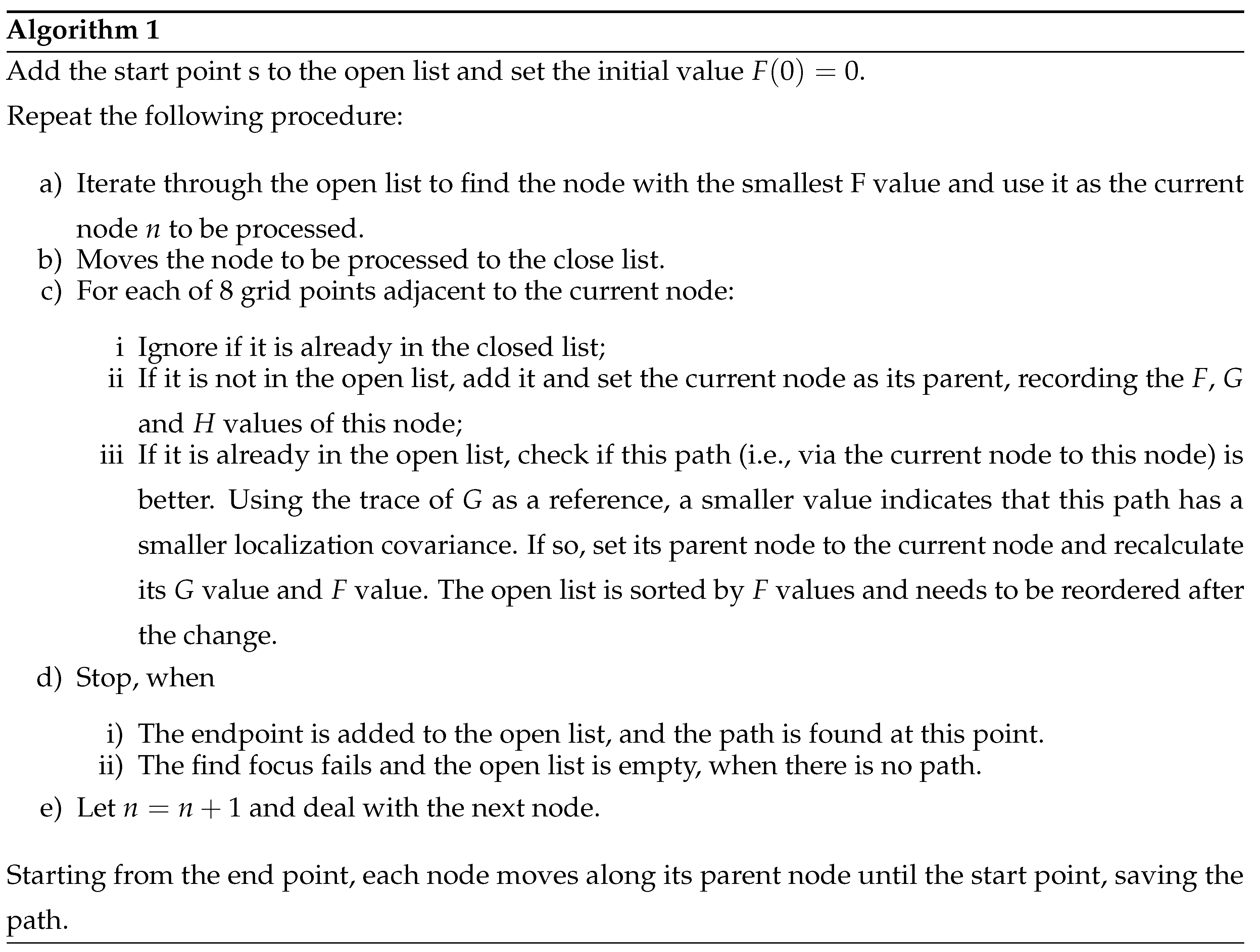
The A* algorithm controls the points in the map by setting the open list and close list. The pseudo code table of PCRB-based A* path planning algorithm is as follows:
4. Simulation
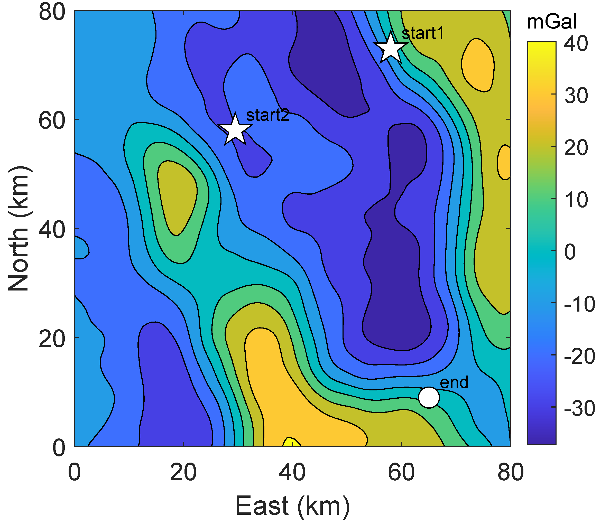
The numerical gravity map of the simulation shown in
Figure 2 is derived from the global ocean gravity field
model produced by Sandwell’s team [
31], and the accuracy of the gravity field of the selected experimental region is better than
. The maximum gravity anomaly in the region is
and the minimum is
. The gravity anomaly is highly undulating and contains various topographic features such as peaks, slopes, and flats, which are suitable for path planning analysis. Since the actual horizontal distances of longitude and
latitude of
are different, in order to unify the navigation errors, this paper converts the earth coordinates into geographic coordinates centered on the map center position through equation (
31) and equation ()
where
is the eastward distance from the center of the map and
is the northward distance from the center of the map.
is the latitude of the coordinate origin. Earth’s radius (long semi-axis)
. Oblateness of the earth
. The radius of principal curvature of the meridian circle
. The radius of the Earth’s circle of latitude
. And then the origin is shifted to the lower left corner of the map to get the
Figure 2, and the spatial resolution of the map after interpolation is
.
The measure of trajectory performance uses the Root Mean Square Error (RMSE), which is the square root of the ratio of the square of the deviation of the predicted value from the true value to the number of observations
n.
where
is the estimated value of the trajectory heading coordinates,
is the true value of the trajectory heading coordinates, and N is the number of Monte Carlo experiments.
The estimated coordinates
are calculated using the SITAN algorithm, which is essentially an extended Kalman filter algorithm. The state error propagation is
where
is the position error of INS, i.e.
.
SITAN fits a linear observation model using stochastic linearization techniques
The fitting expression for
in the observed model is
(
36) and () describe the process of calculating the observation matrix
H for gravity anomaly data. The variables used are:
which represents the grid of the INS indicator position on the digital gravity map;
which is the gravity anomaly extracted from the digital map based on the INS indicated position;
which is the gravity anomaly measured in real-time;
which is the spacial resolution of the digital map; and
L which represents the number of grid points in the length of the fitted interval.
The center point of the fitted region is the INS position, and the size of the region is determined by the position error covariance of INS. To calculate the observation matrix H, gravity anomaly values of all grid points in the region are used. Generally, a more accurate INS indicator position leads to a smaller INS confidence interval, resulting in a more precise linearized observation model.
4.1. Test 1
The starting point (start1) of Test 1 in the planned path is located at
in
Figure 2. The point is located within the slope area, where contour lines are densely distributed. The ending point, on the other hand, has coordinates of
.
Table 1 lists the simulation conditions.
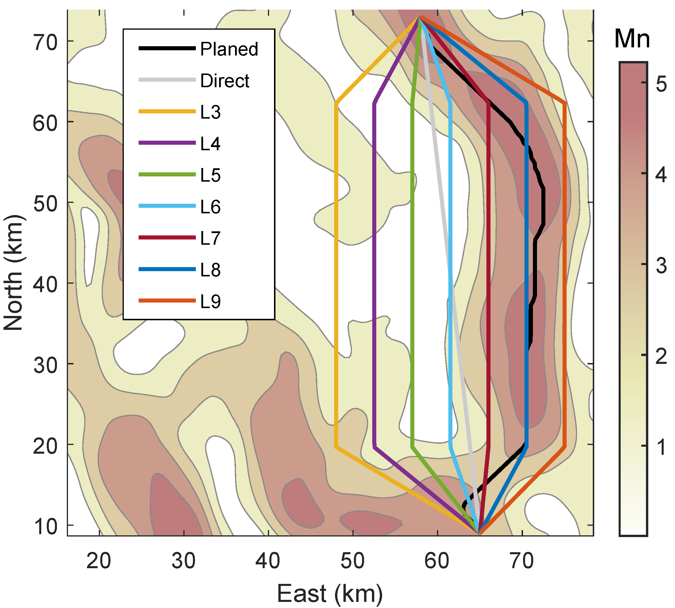
Figure 3 displays the contours of Mn, calculated from equation (
19). A comparison between this and the gravity anomaly contours in
Figure 2 reveals that regions with denser contours correspond to larger Mn. This suggests that more gravity information is available in such areas.
Following the proposed method, the planned path intersects the region with maximum information. To determine the optimality of the planned path, we established several equally spaced curves for comparison, including the shortest Direct path and seven others labelled L3, L4, ... ,L9, from left to right. The paths are shown in
Figure 3. We conducted 1000 random simulations using the Monte Carlo method and identical parameters as those outlined in
Table 1. Each trajectory was divided into 100 sampling points by equal Euclidean distances.
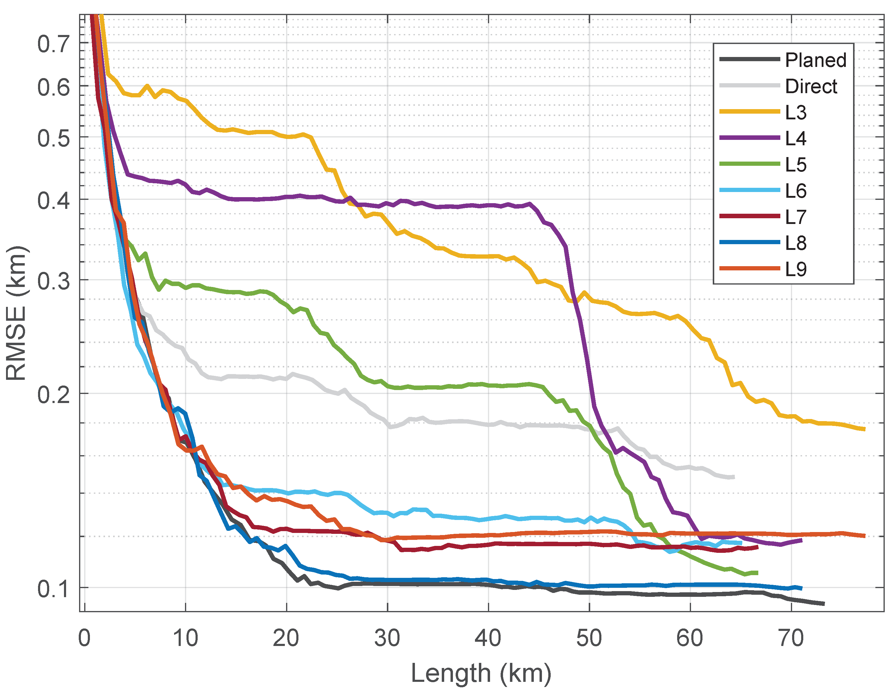
Figure 4 provides a comparison of the localization accuracy achieved using different trajectories in Test 1. As can be seen from
Figure 4, the RMSE of all paths decreases rapidly during the initial stage since the starting point 1 is located in a region with high Mn values. However, the planned trajectory outperforms all other paths in terms of localization accuracy.
The black curve represents the planned path, while the gray curve denotes the straight-line path. Although the planned trajectory covers approximately more distance than the straight-line trajectory, the RMSE converges fastest with the path length when sailing along the planned path. Moreover, the RMSE remains the lowest among all paths, with convergence accuracy stabilizing around after reaching .
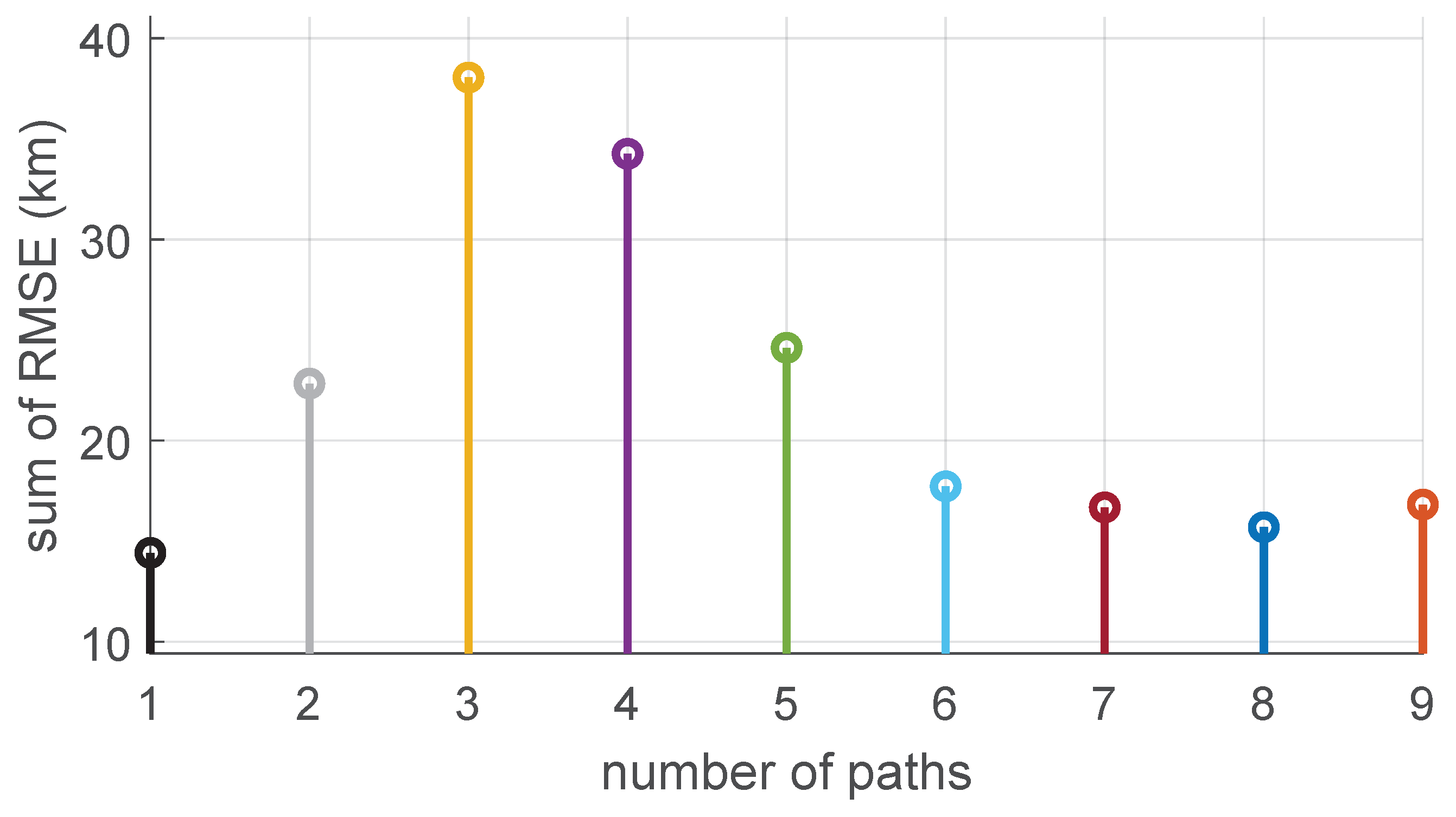
The sum of RMSE of the trajectories are shown in
Figure 5. Among all the trajectories, L8 shows the closest trace to the planned path, including partial path overlap. However, the trend of RMSE for these four trajectories is similar, with the planned trajectory exhibiting the smallest value. L7 and L9 also show good positioning accuracy, indicating that the trajectories near the planned path can also achieve high localization accuracy. Nevertheless, the planned path remains the better choice as it exhibits the highest positioning accuracy. Furthermore, the planned path maintains reliable positioning accuracy between L7 and L9, even if it deviates from the intended route. This ensures that the carrier does not get lost, reducing the risk of losing the carrier significantly. The planned trajectory is the optimal choice since it offers both high localization accuracy and reliability in maintaining this accuracy, especially in regions with high Mn values.
4.2. Test 2
Test 1 indicates that the RMSE of all trajectories decreases rapidly during the initial phase because the starting point is located in a gravity informative region. Test 2 changed the starting point (start2) to
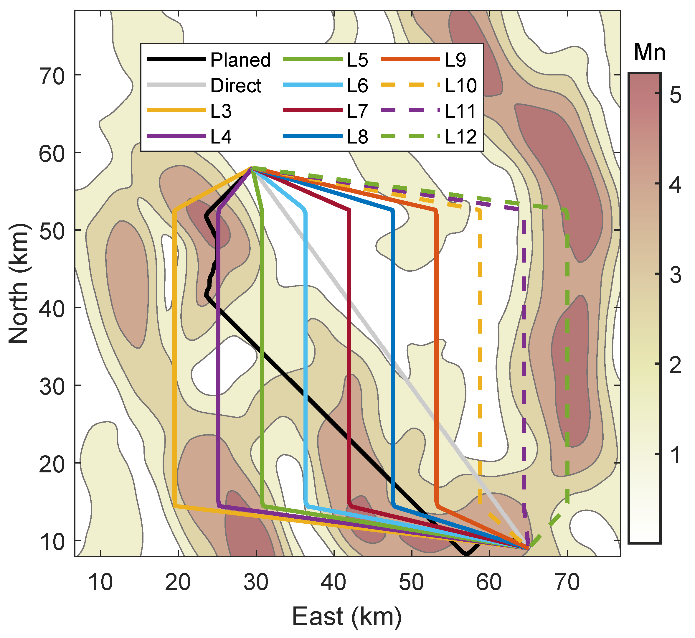
, situated at a relatively gentle seabed. As shown in
Figure 6, this location has a smaller Mn value, indicating that less gravity information can be used at the initial position. In the figure, the black curve represents the planned trajectory, while the gray curve represents the direct trajectory.
To further Test the proposed method, we generated 10 additional paths between the starting and ending points, with each path having a lateral distance of
. All 12 trajectories are depicted in
Figure 6, where the black curve corresponds to the planned path, while the gray Direct path represents the shortest path directly connecting the starting and ending points. We named these newly added paths from left to right as L3, L4, ..., L12, and each trajectory is divided into 100 sampling points by equal Euclidean distance.
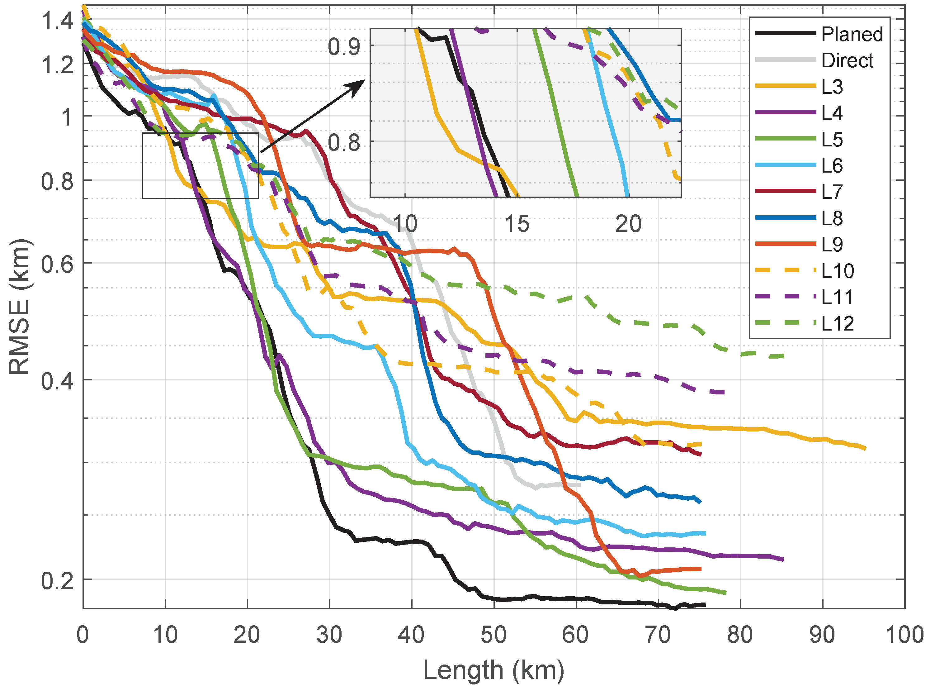
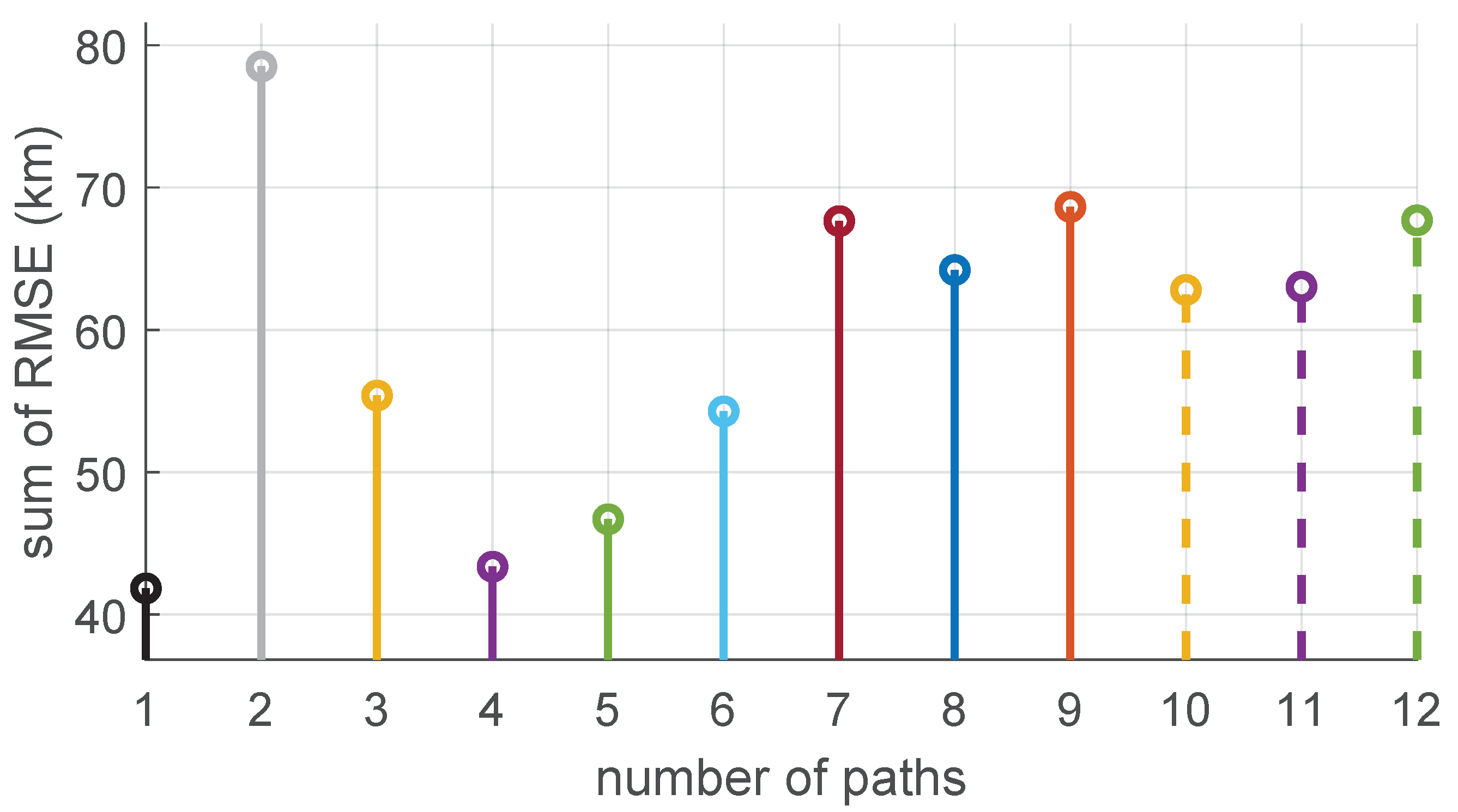
Figure 6 displays the distribution of 12 trajectories. The RMSE of the position error for these trajectories is plotted in
Figure 7, while the sum of RMSE values for each trajectory is presented in
Figure 8. The starting point of Test 2 is situated in an area with a small Mn value. In addition to the planned trajectory, there are two lines, L3 and L4, through the region with large Mn values on the left areas. Among all lines, L4 shows a long overlap with the planned trajectory during its initial phase. From
Figure 7, it can be observed that the RMSE of the planned trajectory, L3, and L4 decreases the fastest. These three trajectories have an RMSE of approximately
at a trajectory length of 15 km. Line L5 also passes through a large Mn area but not as much as L3, L4, and the planned trajectory. Therefore, its positioning error decreases faster than other trajectories after the three.
However, the remaining trajectories, L6-L12 and the direct trajectory, exhibit a bias towards the east in the beginning phase, resulting in slower decrease of their position errors. The RMSE of the planned trajectory reaches minimum at
, followed by maintaining convergence. The speed of convergence and convergence down line of the planned trajectory are significantly better than the other trajectories. Furthermore, the sum of RMSE of the planned trajectory, presented in
Figure 8 is
, which makes it the optimal path among all 12 trajectories. L4 has the second-best performance, with an RMSE of
. On the other hand, the direct trajectory exhibits a disappointing performance, with a large position error located in the region of very small Mn values in the beginning stage. Its RMSE curve decreases slowly, and the sum of RMSE is the largest among all trajectories, reaching
. Hence, these results indicate that the positioning accuracy in the initial stage holds a significant influence on the RMSE of the entire path.
4.3. The impact of Changing the Measurement Noise on the Paths
In practice, the statistical characteristics of gyroscope and accelerometer noise in inertial navigation systems are usually known and stable after careful calibration, so the process noise is stable. Therefore, the main factor to consider is the impact of gravity measurement errors. And since gravity measurement noise is affected by carrier motion, waves, and inaccurate map modeling, its variance is difficult to estimate accurately, so path planning should be considered to adapt to different measurement noise. The calculation of the sum of RMSE of two experimental trajectories is carried out by changing the standard deviation of the measurement noise
to obtain
Table 2.
In an overall view in
Table 2 and
Table 3, increasing the amount of measurement noise will increase the lower limit of positioning error, but will not change the ranking of the lower limit size of the curve, so the planned trajectory always has higher positioning accuracy than the other curves. Therefore, the planned trajectory is always optimal. And with the increase of the measurement noise, the improvement of the localization accuracy of the planned trajectory is more obvious. The optimality of the planned trajectory is not affected by gravimetric measurements, so that the planned trajectory can be navigated in one determined ocean mission to achieve the optimal navigation accuracy. In addition, the RMSE of a spatially close trajectory to the planned path is also close to the RMSE of the planned trajectory. Therefore, even if the real path deviates from the planned one by a small amount, it is possible to obtain a high positioning accuracy by gravity information.
5. Conclusions
This article proposed a method to plan a path that aims for the best positioning accuracy by using the Postiori Cramer-Rao bound of Gravity-aided Inertial Navigation System as the cost value in the A* algorithm. This path planning method is not limited by the ocean gravity field and can plan the trajectory with the minimum navigation error between any start and end points. The next work is to find the set of trajectories within a certain error requirement in which the carrier can achieve higher positioning accuracy without strictly following a certain trajectory, thereby improving the mobility of the carrier.
Author Contributions
Conceptualization, B.W.; methodology, B.W.; software, B.W.; validation, B.W.; formal analysis, B.W.; investigation, B.W.; resources, B.W.; data curation, B.W.; writing—original draft preparation, B.W.; writing—review and editing, B.W.; visualization,B.W.; supervision, T.C.; project administration,T.C.; funding acquisition, T.C.. All authors have read and agreed to the published version of the manuscript.
Funding
This research was funded by the National Key R&D Program of China, Grant Nos. 2017YFC0601601.
Institutional Review Board Statement
Not applicable.
Informed Consent Statement
Not applicable.
Data Availability Statement
For the results and data generated during the study, please contact the corresponding author.
Conflicts of Interest
The authors declare no conflict of interest.
Abbreviations
The following abbreviations are used in this manuscript:
| GAINS |
Gravity-aided inertial navigation system |
| INS |
Inertial Navigation System |
| PCRB |
Postiror Cramér-Rao bound |
| RMSE |
Root Mean Square Error |
References
- Huang, H.; Tang, J.; Liu, C.; Zhang, B.; Wang, B. Variational Bayesian-Based Filter for Inaccurate Input in Underwater Navigation. IEEE Transactions on Vehicular Technology 2021, 70, 8441–8452. [Google Scholar] [CrossRef]
- Bao, J.; Li, D.; Qiao, X.; Rauschenbach, T. Integrated navigation for autonomous underwater vehicles in aquaculture: A review. Information Processing in Agriculture 2020, 7, 139–151. [Google Scholar] [CrossRef]
- Jalal, F.; Nasir, F. Underwater Navigation, Localization and Path Planning for Autonomous Vehicles: A Review. 2021 International Bhurban Conference on Applied Sciences and Technologies (IBCAST), 2021, pp. 817–828. [CrossRef]
- Liu, H.; Wu, L.; Bao, L.; Li, Q.; Zhang, P.; Xi, M.; Wang, Y. Comprehensive Features Matching Algorithm for Gravity Aided Navigation. IEEE Geoscience and Remote Sensing Letters 2022, 19, 1–5. [Google Scholar] [CrossRef]
- Wang, Z.; Huang, Y.; Wang, M.; Wu, J.; Zhang, Y. A Computationally Efficient Outlier-Robust Cubature Kalman Filter for Underwater Gravity Matching Navigation. IEEE Transactions on Instrumentation and Measurement 2022, 71, 1–18. [Google Scholar] [CrossRef]
- Wang, B.; Ma, Z.; Huang, L.; Deng, Z.; Fu, M. A Filtered-Marine Map-Based Matching Method for Gravity-Aided Navigation of Underwater Vehicles. IEEE/ASME Transactions on Mechatronics 2022, 27, 4507–4517. [Google Scholar] [CrossRef]
- Gao, S.; Cai, T.; Fang, K. Gravity-Matching Algorithm Based on K-Nearest Neighbor. Sensors 2022, 22. [Google Scholar] [CrossRef] [PubMed]
- Stepanov, O.; Nosov, A. Algorithm for Planning an Informative Route for Map-Aided Navigation. 2021 28th Saint Petersburg International Conference on Integrated Navigation Systems (ICINS), 2021, pp. 1–5. [CrossRef]
- Liu, F.; Li, F.; Jing, X. Navigability Analysis of Local Gravity Map With Projection Pursuit-Based Selection Method by Using Gravitation Field Algorithm. IEEE Access 2019, 7, 75873–75889. [Google Scholar] [CrossRef]
- Feng, X.; Wang, B.; Deng, Z.; Fu, M. Internal path planning method for underwater vehicle with gravity aided navigation. 2016 35th Chinese Control Conference (CCC), 2016, pp. 5537–5541. [CrossRef]
- Yang, J.; Huo, J.; Xi, M.; He, J.; Li, Z.; Song, H.H. A Time-Saving Path Planning Scheme for Autonomous Underwater Vehicles With Complex Underwater Conditions. IEEE Internet of Things Journal 2023, 10, 1001–1013. [Google Scholar] [CrossRef]
- Wang, B.; Cai, T.; Fang, K. The Quantification Method of Matching Capability of Areas in Gravity-Aided Inertial Navigation. IEEE Sensors Journal 2022, 22, 20958–20967. [Google Scholar] [CrossRef]
- Stepanov, O.A.; Nosov, A.S.; Toropov, A.B. Navigation informativity of geophysical fields in map-aided navigation. 2017 DGON Inertial Sensors and Systems (ISS), 2017, pp. 1–19. [CrossRef]
- Panda, M.; Das, B.; Subudhi, B.; Pati, B.B. A Comprehensive Review of Path Planning Algorithms for Autonomous Underwater Vehicles. Int. J. Autom. Comput. 2020, 17, 321–352. [Google Scholar] [CrossRef]
- Sang, H.; You, Y.; Sun, X.; Zhou, Y.; Liu, F. The hybrid path planning algorithm based on improved A* and artificial potential field for unmanned surface vehicle formations. Ocean Engineering 2021, 223, 108709. [Google Scholar] [CrossRef]
- Chong, Y.; Chai, H.; Li, Y.; Yao, J.; Xiao, G.; Guo, Y. Automatic Recognition of Geomagnetic Suitability Areas for Path Planning of Autonomous Underwater Vehicle. Marine Geodesy 2021, 44, 287–305. [Google Scholar] [CrossRef]
- Ma, Y.; Gong, Y.; Xiao, C.; Gao, Y.; Zhang, J. Path Planning for Autonomous Underwater Vehicles: An Ant Colony Algorithm Incorporating Alarm Pheromone. IEEE Transactions on Vehicular Technology 2019, 68, 141–154. [Google Scholar] [CrossRef]
- Wang, L.; Liu, L.; Qi, J.; Peng, W. Improved Quantum Particle Swarm Optimization Algorithm for Offline Path Planning in AUVs. IEEE Access 2020, 8, 143397–143411. [Google Scholar] [CrossRef]
- Wang, B.; Zhu, Y.; Deng, Z.; Fu, M. The Gravity Matching Area Selection Criteria for Underwater Gravity-Aided Navigation Application Based on the Comprehensive Characteristic Parameter. IEEE/ASME Transactions on Mechatronics 2016, 21, 2935–2943. [Google Scholar] [CrossRef]
- Wang, B.; Zhou, M.; Deng, Z.; Fu, M. Sum Vector-Difference-Based Matching Area Selection Method for Underwater Gravity-Aided Navigation. IEEE Access 2019, 7, 123616–123624. [Google Scholar] [CrossRef]
- Bergman, N. Recursive bayesian estimation: Navigation and tracking applications. PhD thesis, Linkoping University, 1999.
- Tichavsky, P.; Muravchik, C.; Nehorai, A. Posterior Cramer-Rao bounds for discrete-time nonlinear filtering. IEEE Transactions on Signal Processing 1998, 46, 1386–1396. [Google Scholar] [CrossRef]
- Zhong, X.; Premkumar, A.B.; Madhukumar, A.S. Particle Filtering and Posterior Cramér-Rao Bound for 2-D Direction of Arrival Tracking Using an Acoustic Vector Sensor. IEEE Sensors Journal 2012, 12, 363–377. [Google Scholar] [CrossRef]
- Hernandez, M.; Farina, A. PCRB and IMM for Target Tracking in the Presence of Specular Multipath. IEEE Transactions on Aerospace and Electronic Systems 2020, 56, 2437–2449. [Google Scholar] [CrossRef]
- Lee, H.; Chun, J.; Jeon, K. Experimental Results and Posterior Cramér–Rao Bound Analysis of EKF-Based Radar SLAM With Odometer Bias Compensation. IEEE Transactions on Aerospace and Electronic Systems 2021, 57, 310–324. [Google Scholar] [CrossRef]
- Zhang, S.; Chen, D.; Fu, T.; Cao, H. Approximating Posterior Cramér–Rao Bounds for Nonlinear Filtering Problems Using Gaussian Mixture Models. IEEE Transactions on Aerospace and Electronic Systems 2021, 57, 984–1001. [Google Scholar] [CrossRef]
- OuYang, M.; Ma, Y. Path planning for gravity aided navigation based on improved A* algorithm. Chinese J. Geophys 2020, 63, 4361–4368. [Google Scholar] [CrossRef]
- Liu, X.; Ma, D.; Yang, M.; Xia, X.; Guo, P. Modified Block A* Path-Planning Method for Hybrid-Driven Underwater Gliders. IEEE Journal of Oceanic Engineering 2022, 47, 20–31. [Google Scholar] [CrossRef]
- Anderson, R.C.; Davenport, J.A.; Jekeli, C. Determination of Gravity Data Spacing Required For Inertial Navigation. Navigation 2000, 47, 1–6. [Google Scholar] [CrossRef]
- Higham, N.J. Accuracy and Stability of Numerical Algorithms, second ed.; Society for Industrial and Applied Mathematics, 2002; p. 258. [CrossRef]
- Sandwell, D.; Garcia, E.; Soofi, K.; Wessel, P.; Chandler, M.; Smith, W.H.F. Toward 1-mGal Accuracy in Global Marine Gravity from CryoSat-2, Envisat, and Jason-1. The Leading Edge 2013, 32, 892–899. [Google Scholar] [CrossRef]
|
Disclaimer/Publisher’s Note: The statements, opinions and data contained in all publications are solely those of the individual author(s) and contributor(s) and not of MDPI and/or the editor(s). MDPI and/or the editor(s) disclaim responsibility for any injury to people or property resulting from any ideas, methods, instructions or products referred to in the content. |
© 2023 by the authors. Licensee MDPI, Basel, Switzerland. This article is an open access article distributed under the terms and conditions of the Creative Commons Attribution (CC BY) license (http://creativecommons.org/licenses/by/4.0/).
