Synchronization, Control and Data Assimilation of the Lorenz System

Preprint

Article

Synchronization, Control and Data Assimilation of the Lorenz System

This version is not peer-reviewed.

This version is not peer-reviewed.

Altmetrics

Downloads

112

Views

Comments

Submitted:

06 April 2023

Posted:

07 April 2023

You are already at the latest version

A peer-reviewed article of this preprint also exists.

Abstract

We explore several aspects of replica synchronization with the goas of retrieving the value of parameters for the Lorenz system. The idea is that of having a computer replica (slave) of a natural system (master, simulated in this paper), and exploit the fact that slave synchronizes with the master only if they evolve with the same parameters. As a byproduct, in the synchronized phase the state variables of the slave and that of the master are the same, thus allowing to perform measurements impossible on the real system. We review some aspects of master-slave synchronization using a subset of variables, with intermittent coupling. We show how synchronization can be achieved when some of the state variables are available for direct measurement using a simulated annealing approach, and also when they are accessible only through a scalar function, using a pruned-enriching ensemble approach, similar to genetic algorithms without cross-over.

Keywords:

Subject:

Physical Sciences - Theoretical Physics

1. Introduction

There are many cases in which one is interested in forecasting the behaviour of a chaotic system, the emblematic one is meteorology. The main obstacle is, of course, that in chaotic systems by definition a small uncertainty amplify exponentially in time [1]. Moreover, even if one assumes to have a good computational model of a natural, chaotic system, the exact value of parameters is needed to have a faithful representation of dynamics.

Schematically, one can assume that the natural, or target system is well represented by some dynamical system, possibly with noise. One can measure some quantities on this system, but in general one is not free to choose which variable (or combination of variables) to measure nor to perform measurements at any rate.

On the other hand, if one has a good knowledge of the system under investigation, i.e., it can be modeled with good accuracy, a simulated “replica” of the system can be implemented on a computer. If moreover one has the possibility of knowing the parameters and the initial state of the original system, so to keep the replica synchronized to it (when running at the same speed), then the replica can be used to perform measurements otherwise impossible, and to get accurate forecasting (when run at larger speed).

In general, the problem of extracting the parameters of a system from a time-series of measurement on it, is called data assimilation [2].

The problem in data assimilation is that of determining the state of the system and the parameters by minimizing an error function between data measured on the target and the respective data from the simulated system. A similar task is performed by the back-propagation techniques in machine learning [3,4].

The goal of this paper is that of approaching this problem from the point of view of dynamical systems [5]. In this context the theme of synchronization is quite explored [6], but it has to be extended in order to cover the application field of data assimilation.

The synchronization technique is particularly recommendable when the noise (in the measure and intrinsic to the system) is small, i.e., when the target system can be assumed to be well represented by a deterministic dynamics, even if this dynamics is not continuous (as in Cellular Automata [7]).

We shall investigate here the application of synchronization methods to the classic Lorenz system [8].

We shall start from the classic Pecora-Carrol master-slave synchronization scheme, recalled in Section 2, in which the value of some of the state variables of the master is imposed to the corresponding variables of the slave system. This choice of coupling variables is denoted “coupling direction” in the tangent space of the system.

The synchronization threshold is connected to the value of the conditional Lyapunov exponent [9,10], i.e., the exponential growing rate along the difference space between master and slave, as reported in Section 3.

This scheme will be then extended to partial synchronization, i.e., to the case in which only a portion of the value of the state variables of the master system signal is fed to the slave, as shown in Section 4. We can thus establish the minimum fraction of signal (coupling strength) able to synchronize the two replicas, that depends on the coupling direction.

However, one cannot pretend to be able to perform measurements in continuous time, as done in the original synchronization scheme, in which the experimental reference system was a chaotic electronic circuit.

Therefore, we dealt with the problem of intermittency, i.e., performing measurements, and consequently applying the synchronization scheme, only at certain time intervals. We show that the synchronization scheme works also for intermittent measurements, provided that the coupling strength is increased, as shown in Section 5.

In the case of systems with different parameters, the synchronization cannot be complete, and we speak of generalized synchronization. We shall show in Section 7 that the distance among systems can be interpreted as measure of the error, and exploited to obtain the “true” value of parameters, using a simulated annealing scheme.

Finally, it may happen that the variables of the systems are not individually accessible to measurements, a situation which forbids the application of the original method. In this case one can still exploit schemes inspired by statistical mechanics, like the pruned and enriching one, simulating an ensemble of systems with different state variables and parameters, and selecting the instances with less error, cloning them with perturbations. This kind of genetic algorithms is able to approximate the actual values of parameters, as reported in Section 8.

Conclusions are drawn in the last section.

2. Pecora-Carrol synchronization

In 1990 Louis Pecora and Thomas Carrol introduced the idea of master-slave synchronization [9]. They studied simulated systems, like the Lorenz [8] and Rössler [11] ones, and also experimental electronic circuits [12].

They considered two replicas of the same system, with same parameters. One of the replica (the master) was left evolving unperturbed. Some of state variables of the master replaced the corresponding variable of the slave system, which is therefore no more autonomous. This topic was further explored in a 2015 paper [10].

In order to get the main idea of this master-slave (or replica) synchronization, let us consider first a one-dimensional, time-discrete dynamical system, like for instance the logistic map [13]. It is defined by an equation of the kind

x_{n + 1} = f (x_{n}),

(1)

where n labels the time interval. The usual Lyapunov exponent

λ

is defined as

λ = lim_{N \to \infty} \sum_{n = 1}^{N} log (f^{'} (x_{n})),

(2)

where

f^{'} (x) = d f / d x

. Let us now introduce a replica X such that

\begin{matrix} x_{n + 1} & = f (x_{n}); \\ X_{n + 1} & = (1 - p) f (X_{n}) + p f (x_{n}), \end{matrix}

(3)

where p is the coupling parameter (coupling strength).

For

p = 0

the two maps are uncoupled, and since they are assumed to be chaotic, they generally take different values. For

p = 1

map X immediately synchronizes with map x. There is a critical value

p_{c}

of the coupling parameter for which the synchronized state is stable, and it is related to the Lyapunov exponent

λ

p_{c} = 1 - exp (- λ),

(4)

as can be seen by taking the linearized difference among the maps.

This scenario holds also for higher-dimensional (K) maps, which can be written as

r_{n + 1} = F (r_{n}),

(5)

where

r_{n}

denotes the state of the system at iteration n and has K components. The system has now K Lyapunov exponents, of which at least one,

λ_{MAX}

, is assumed to be positive.

The synchronization procedure in this case is

\begin{matrix} r_{n + 1} & = F (r_{n}); \\ R_{n + 1} & = (I - p C) F (R_{n}) + p C F (r_{n}), \end{matrix}

(6)

where now the coupling is implemented by means of a diagonal matrix C, with diagonal entries equal to zero or one, defining the coupling directions. In the following we shall indicate the diagonal of C as

C = [c_{x}, c_{y}, c_{z}]

In the case in which

C = I

, i.e., all entries are mixed with the same proportion, the stability of the synchronized phase is again related to the maximum Lyapunov exponent

λ_{MAX}

p_{c} = 1 - exp (- λ_{MAX}),

(7)

since the evolution of an infinitesimal difference among the replicas,

δ

, is given by

δ_{n + 1} = (1 - p) J (x) δ_{n},

(8)

where J is the Jacobian of F

J_{i j} = {(\frac{\partial F_{i}}{\partial x_{j}})}_{x = x_{n}} .

(9)

This scheme can be extended to continuous-time systems, by replacing the entries from one system in the coupled differential equation, so

\begin{matrix} \dot{r} & = F (r); \\ \dot{R} & = (I - p C) F (R) + p C F (r) . \end{matrix}

(10)

where now the Lyapunov exponents of the original system are given by the eigenvalues of the (symmetrized) time-average of Jacobian

Λ

Λ = lim_{t \to \infty} \frac{1}{2 t} (\int_{0}^{t} J (r (t)) + {(\int_{0}^{t} J (r (t)))}^{T}) .

(11)

In practice, however, the differential equation Eq. (10) is implemented as a map, by discretizing the time, and therefore Lyapunov exponents are computed as in the previous case. Using a simple Euler scheme, we have

t = n Δ t

and

r (t) = r (n Δ t) = r_{n}

, and

r_{n + 1} = r_{n} + F (r_{n}) Δ t .

(12)

In the tangent space

δ r_{n + 1} = (1 + J (r_{n}) Δ t) δ r_{n},

(13)

and the maximum Lyapunov exponent

λ_{MAX}

λ_{MAX} = lim_{n \to \infty} \frac{1}{n Δ t} \sum_{n} log (1 + J (r_{n}) Δ t) ≃ lim_{n \to \infty} \frac{1}{n} \sum_{n} J (r_{n}) .

(14)

The average growth of the distance

δ r

δ r (t) = δ_{0} exp (λ_{MAX} n Δ t) = exp (λ_{MAX} t),

(15)

for time intervals such that the linearized approximation is valid.

Notice that in the continuous-time version the Jacobian and the Lyapunov exponents are defined in units of the inverse of time.

3. Conditional coupling

In the original Pecora-Carrol implementation [10], the signal from the master is fully extracted , i.e.,

p = 1

, so that for the

R

system, either a component is untouched, or it is derived from the replica (

r

To be explicit, for the Lorenz system we have

\begin{matrix} \dot{x} & = σ (y - x), \\ \dot{y} & = - x z + ρ x - y, \\ \dot{z} & = x y - β z . \end{matrix}

(16)

For instance, for a full coupling along the x direction (

C = [1, 0, 0]

), the replica will follow the equation

\begin{matrix} X & = x, \\ \dot{Y} & = - x Z + ρ x - Y, \\ \dot{Z} & = x Y - β Z . \end{matrix}

(17)

It is possible to define the sub-Lyapunov [9] or, better, the conditional Lyapunov exponents [10], by iterating the equation for the difference

δ r

in the tangent space. For instance, for the Lorenz system coupled along the x direction (

C = [1, 0, 0]

), we have

\frac{d}{d t} (\begin{matrix} δ y \\ δ z \end{matrix}) = (\begin{matrix} - 1 & - x \\ x & - β \end{matrix}) \cdot (\begin{matrix} δ y \\ δ z \end{matrix}),

(18)

giving two conditional exponents. The system synchronizes if both of them are negative.

Figure 1 we report the value of the maximum conditional Lyapunov exponent as a function of the coupling strength p for the

C_{x} = [1, 0, 0]

C_{y} = [0, 1, 0]

and

C_{z} = [0, 0, 1]

coupling directions.

As noted also in Ref [10], the Lorenz system synchronizes if coupled along the x and y directions, but not along the z one, even for

p = 1

Our observable was the average distance d,

\begin{matrix} d (t) & = | | r (t) - R (t) | | = \sqrt{{(x (t) - X (t))}^{2} + {(y (t) - Y (t))}^{2} + {(z (t) - Z (t))}^{2}}, \\ d & = \frac{1}{T} \int_{0}^{T} d (t) d t, \end{matrix}

(19)

computed after a proper transient.

In Figure 2 we show d as a function of the coupling strength p for different coupling directions. For all the simulations we set

σ = 10

β = 8 / 3

ρ = 28

, and we use the Euler integration scheme to integrate the equation with temporal step

d t = 10^{- 3}

. After a transient time of free evolution we couple the master and the slave system every time step. At

T = 100

(simulation end time) we compute the distance d between the two systems.

4. Partial conditional coupling

We can naturally generalize the definition of maximum conditional Lyapunov exponents also when we do not have a full coupling, i.e.,

p < 1

, looking for the synchronization threshold

p_{c}

, for which

d (p)

goes to zero.

From the plots reported in Figure 2, one can see that for the x and y coupling there is a well defined synchronization threshold, similar to that obtained for the uniform coupling. For the z coupling, the maximum Lyapunov exponent is always positive (albeit small), and no synchronization is possible.

This behaviour is showed in Figure 1, were we plot the maximum conditional Lyapunov exponent for different coupling strength p and different coupling direction C. For the z coupling, we also plot the distance

d (p)

for some p (as Figure 2).

One can see also that in the un-synchronized phase, the distance

d (p)

exhibits a non-monotonous behavior, except in the vicinity of the synchronization transitions, Figure 2. This aspect will be analyzed in Section 7.

5. Intermittent synchronization

In real applications, it is generally impossible to get a signal from one system and inject it into the replica in a time-continuous way. Pecora and Carrol were able to do it using electronic circuits [9], but if one need to pass through a measurement system, it is expects that this device has a finite bandwidth, i.e., a finite measurement time.

So the question becomes: is it possible to synchronize two replicas measuring one quantity only at time intervals

τ

Numerically, if the equations are integrated using a constant time step

Δ t

, this means that the replacement or mixing of components is applied every k time steps, so that

τ = k Δ t

For homogeneous coupling (

C = [1, 1, 1]

), the linear analysis for simply tells that (Equation 7)

p_{c} = 1 - exp (- λ_{MAX} Δ t \cdot k) = 1 - exp (- λ_{MAX} τ),

(20)

i.e., intermittent synchronization is equivalent to the standard synchronization for a system with a larger Lyapunov exponent.

Then, for small

τ

, we have

p_{c} = λ_{MAX} τ .

(21)

This relationship holds numerically also for other coupling directions, as shown in Figure 3. In the figure we also plot the linear fit obtained using the first 20 points.

The estimated values obtained from the linear fit (

λ_{fit}

), compared with the values (

λ_{lin}

) computed using equation 21 with

p_{c}

estimated numerically (Figure 2), are summarized in Table 1.

6. Generalized synchronization

What happens if the two coupled replicas evolve using different values of parameters

σ, ρ, β

[6,14]? Even when the coupling parameters (directions and intensity) are above threshold, the distance d remains finite. Let us indicate with

σ^{'}, ρ^{'}, β^{'}

the parameters of the slave system.

We can define a parameter distance D,

D = \sqrt{{(σ - σ^{'})}^{2} + {(ρ - ρ^{'})}^{2} + {(β - β^{'})}^{2}},

(22)

which is zero for the previous coupling schemes. We can also generalize the coupling among replicas, similar to what done for state variables, Eq.(6), introducing a parameter coupling direction

χ = [χ_{σ}, χ_{ρ}, χ_{β}]

and a strength

π

so that the parameters of the slave replica are

\{\begin{matrix} σ^{'} = σ + χ_{σ} π (σ_{1} - σ), \\ ρ^{'} = ρ + χ_{ρ} π (ρ_{1} - ρ), \\ β^{'} = β + χ_{β} π (β_{1} - β), \end{matrix}

where

σ_{1}, ρ_{1}, β_{1}

are the values of parameters corresponding to

π = 1

, reachable according to the “direction”

χ

We can notice that the distance among state variables d decreases smoothly with

p - p_{c}

and D only for a small interval of D near zero. Clearly,

d > 0

for

p < p_{c}

, even for

D = 0

, which is what we have seen in Section 4.

Some simulation results are presented in Figure 4, in which the asymptotic state-variable distance d is reported as a function of the distance between parameters

D = π D_{0}

and state-variable coupling p. The parameter coupling

π

always goes from 0 to 1, so the initial parameter distance

D_{0}

corresponds to the larger value of D. The line

D = 0

corresponds to the distance reported in Figure 5.

Clearly, in the absence of synchronization for

D = 0

(

C = [0, 0, 1]

, Figure 5-(c)), there is no synchronization for

D > 0

. In the other cases, there is a region near the synchronized phase in which d goes smoothly to zero. Notice that in Figure 5-(c) the larger distance d occurs for

p = 1

and large D. This is probably due to the fact that when coupled along the z directions, the two replicas may stay on different “leaves” of the attractor, which is almost perpendicular to z.

Notice also that the d landscape is not smooth far from the synchronized phase. We consider this aspect in the following section.

7. Parameter estimation

We are now able to exploit the fact the the distance d goes to zero if

p > p_{c}

and

D = 0

, thus allowing to determine the parameters of the master system

r

by varying the parameters of the simulated replica

R

However, since the convergence of d to zero is not monotonous with D, we relay of a simulated annealing technique [15], that allows to overcome the presence of local minima. We introduce a fictitious temperature

θ

, and assume that the distance d is the analogous to an energy to be minimized.

We assume that the the synchronization time

τ

and the coupling direction C, cannot be modified at will by experimenters, being fixed by the characteristic of the measure instruments and of the actuators. We insure to be in the condition

p > p_{c}

, i.e., such that if the parameter distance is null,

D = 0

, synchronization occurs.

The idea is the following: we simulate the coupled system for a time interval T, measuring the state variable distance d, after which one of the parameter

σ, ρ, β

is varied by a small amount. We repeat the simulation starting from the same conditions, except the varied parameter, and compute again d. If d decreases the variation is accepted. It is also accepted if d increases, with a probability

p_{acc} = exp (- \frac{Δ d}{θ}),

(23)

otherwise it is discarded.

The temperature

θ

is slowly lowered (multiplying

θ

by a factor

1 - ϵ

) every T time interval. As shown in Figure 5, in this way it is possible to exploit the synchronization procedure to get the value of the parameters in the master replica. In fact, for

θ

sufficiently low, the distance

| d |

between master and slave state variables (dashed line in figure) drops to zero. For similar values of temperature (but not always the same), also the distances

| Δ |

between master and slave parameters drop to zero (continuous color lines). Clearly, this procedure works only for deterministic dynamical systems with little or no noise on measurement, and with very low dimensionality.

8. Pruned-enriching approach

The previous scheme cannot be always followed, since we assumed to be able to measure some of the variables of the master system and inject this value (at least intermittently) in the slave one.

However, this might be impossible, either because the state variables

x, y, z

are not accessible individually, or because those that are accessible do not allow the synchronization (for instance, if only the z variable is accessible, as illustrated in Section 4).

We can take profit of the Takens theorem [16], that states that the essential features (among which the maximum Lyapunov exponent) of a strange attractor

{r (t)}_{t \to \infty}

can be reconstructed by intermittent observations

w_{n} = f (r (n Δ T))

using the time series

w_{n}, w_{n - 1}, w_{n - 2}, . . .

as surrogate data, provided that their number is larger than the dimensionality of the attractor [17]. Other conditions are that the observation interval

Δ T

be large enough to have observations

w_{n}

sufficiently spaced, but not so large that the

w_{n}

are scattered along the attractor, making the reconstruction of the trajectory impossible. It is therefore generally convenient to take an interval

Δ t

substantially larger than the minimum

Δ t = τ

, but of the same order of magnitude.

What is interesting, is that one can choose for f an arbitrary function of the original variables, provided that their correspondence is smooth. We therefore employed a method inspired by the pruned-enriching technique [18,19] or genetic algorithm without cross-over [20].

We assume that we can only measure a function

f (x, y, z) = f (r)

of the master system, at time intervals

τ

. The master system evolves with parameters

q = (σ, ρ, β)

We simulate an ensemble

{R_{i}}_{i = 1, \dots, h}

composed by h replicas, each one starting from state variables

R_{i} (0)

(

i = 1, \dots, h

) and evolving with the same equation as the master one with parameters

{Q_{i}}_{i = 1, \dots, h}

, where

Q_{i} = (σ_{i}, ρ_{i}, β_{i})

. At beginning

R_{i} (0)

and

Q_{i}

are random quantities.

We let the ensemble evolve for a time interval T and then we measure the distance

d_{i} = | f (r (T)) - f (R_{i} (T)) |

. We sort the replicas according with

d_{i}

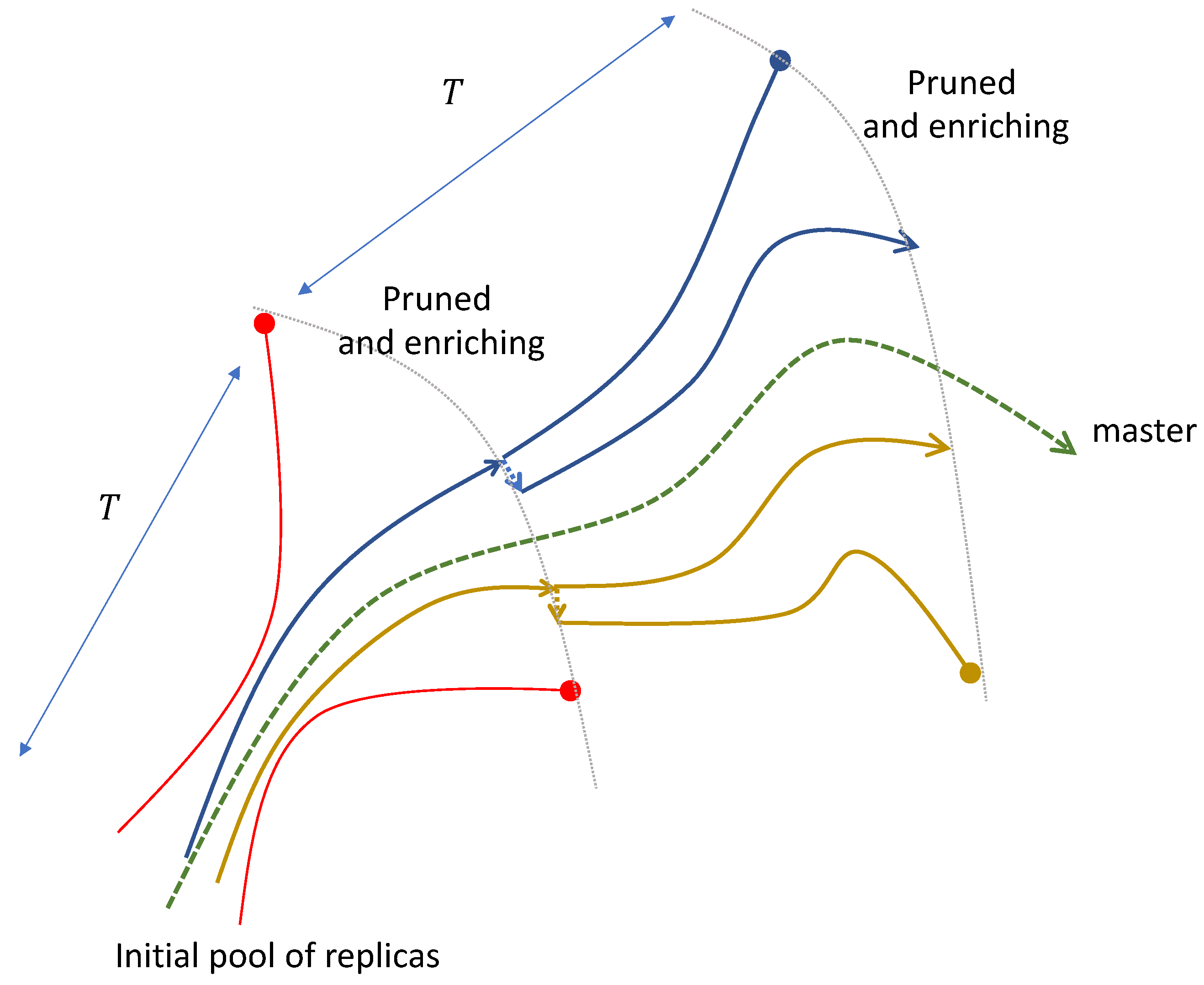
and we replace the half with larger distances following an evolutionary law based on a cloning and perturbation scheme, as shown in Figure 6. For a more detailed description of the procedure we can refer to Algorithms 1 and 2.

First of all we need to set the initial condition. Given a set of measures

{f (r (t))} = {f (r_{n})}

, for

t = t_{0}, t_{0} + τ, \dots, t_{0} + n τ, \dots, T

, we map the dynamics in an embedding space of size

d_{e}

defined by the vectors

w_{n} = (f (r_{n}), f (r_{n - 1}), \dots, f (r_{n - d_{e} + 1}))

. Then we randomly initialize the initial conditions

R_{i} (0)

and the initial value of the parameters

Q_{i}

of the h replicas, in a range consistent with the physical values. To create the initial embedding vectors of the replicas, we evolve the ensemble for a time

T_{T r a n s} \geq d_{e} τ

Now we can start with the optimization problem. For a number of repetitions M, we evolve the ensemble using a time step

d t

up to time

t = T

. At each further interval

τ

we update the embedding vector

w_{i}

substituting the oldest measurement with the new one and compute the euclidean distances

d_{i}

between the

W_{i}

and the reference

w (t)

computed on the master system.

The distance

d_{i}

is used as cost function of our optimization problem. In the Parameters updating step of Algorithm 2, we sort the elements of the set in ascending order according to

d_{i}

and replace the second half of the set with a copy of the first half with either a random perturbation of amplitude

δ

in one of the parameters, or a random perturbation of the state variables, see Algorithm 2.

We add some check to be sure to not have inconsistent values of parameters (in our case all the

Q_{i}

need to be positive). After that we compute

\tilde{Q}

, the estimated parameters, as mean of the fist half of the ensemble elements.

Since in general we assume

M > T / d t

, the number of time steps in the simulated trajectories, when

t = T

we restart the ensemble simulation at the initial time step, restoring initial random condition in the state space but without changing the parameters, and we recompute the initial vector

W_{i}

evolving the ensemble member up to time

t = T_{T r a n s}

We analyze the convergence problem for different value of

δ

. We suppose to have access at only the x component of the real system, i.e. our measurement function is simply

f (r) = x

. We evolve the system up to

T = 100

with time step

d t = 0.01

and we measure every

τ = 0.2

. We embed the system in a embedding space of dimension

d_{e} = 5

The ensemble is composed by

h = 10000

replicas and we repeat the procedure for

M = 50000

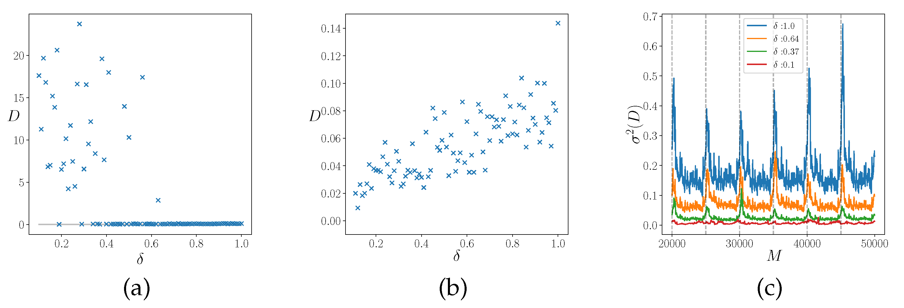
times. The final results are showed in Figure 7. In Figure 7-a we initialize the ensemble parameters randomly in the interval

(0.5, 30)

and we measure the distance D in the parameters space (Eq. (22)) for different

δ

. Notice that, starting from a large initial distance, larger values of

δ

, are more effective for the convergence. The opposite phenomenon is reported in Figure 7-b. Here we assume to approximately know the true parameter values with an error

ϵ

and we test the dependence of the amplitude

δ

in a fine tuning regime. In this case, starting from a relative small distance, smaller values of

δ

are more effective.

In Figure 7-c instead we show the behavior of the variance of the parameter distance D during the optimization for different amplitude

δ

. With a small amplitude

δ

for the parameters updating step, the elements of the ensemble rapidly converge to the local minimum before having explored the parameter space sufficiently so, small amplitude values of

δ

can be useful only for a fine tuning approach. Using large values of

δ

instead is helpful to better explore the parameters landscape and allows to converge to the true values but with noisy results. These considerations suggest the use of an adaptive value of the parameter

δ

Inspired from these results we modify the updating ruled introducing a variable amplitude

δ = (δ_{1}, δ_{2}, \dots, δ_{R})

, where, for every ensemble members i,

δ_{i} = δ_{i} (d_{i})

. Then, for each replica we defined an amplitude that modulates the variation step in an self-consistent manner. To test this choice we simply put

δ_{i} = d_{i} .

(24)

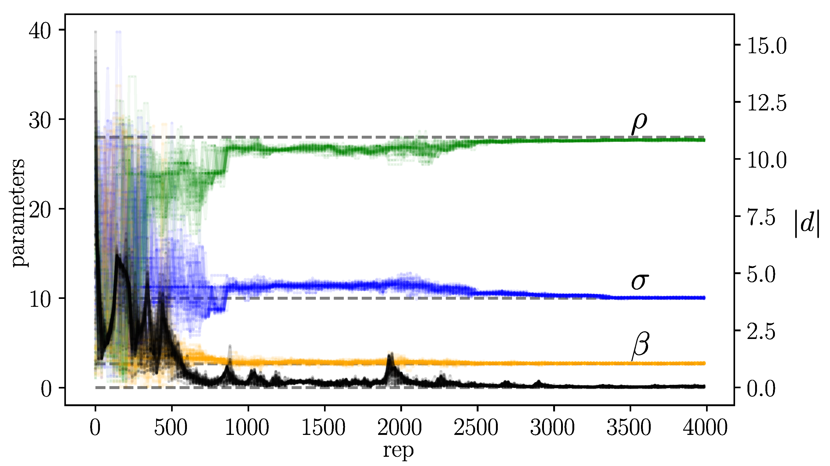
In Figure 8 we plot the behaviour of 50 ensemble members randomly chosen in the pruned-enriching optimization problem with the amplitude factor

δ

defined as in Eq. (24). We suppose to be in the same situation of the last simulations, so we measure the real system only in the

C_{x}

direction every

τ = 0.2

. The ensemble dimension is equal to

h = 10000

and we choose the embedding dimension

d_{e} = 5

. In this simulation we run the algorithm for

M = 80000

intervals. The numerical results as show in Table 2.

Algorithm 1:Pruned-enriching algorithm.

Require: ${w (t)}, δ, Q_{i}, R_{i}, d t, τ, M, T_{T r a n s}$
$m \leftarrow 0$
$t \leftarrow 0$
while $m < M$ do
$m \leftarrow m + 1$
if $t = = T$ then
$t \leftarrow 0$
$W \leftarrow Ensemble evolution up to t = T_{Trans} and store measure every τ$
else
if $t \propto τ$ then
$W \leftarrow Update with f (R)$
$d \leftarrow Euclidean distance d (w (t), W)$
$Q \leftarrow Parameters updating step$ ▹ Algorithm 2
$\tilde{Q} \leftarrow Mean of first R / 2 ensemble elements$
end if
$R \leftarrow Evolution step with time step d t and Q as parameters$
$t \leftarrow t + d t$
end if
end while
return $\tilde{Q}$

Algorithm 2:Parameters updating step.

Require: $R, δ, d, W, w (t)$
$index \leftarrow argsort (d)$ ▹ return index of d sorted in ascending order
for $i in range (R / 2, R)$ do
$Q_{i} \leftarrow Q_{j} with j random integer in (0, R / 2)$
if $random (0, 1) < 0.5$ then
$k \leftarrow random integer in (1, 2, 3)$
$Q_{i k} \leftarrow Q_{j k} + random (- δ, δ)$
while $Q_{i k} < 0$ do
$Q_{i k} \leftarrow Q_{j k} + random (0, δ)$
end while
else
$R_{i k} \leftarrow R_{j k} + random (- δ, δ)$
end if
end for
return $Q$

The pruned-enriching procedure is similar to a genetic algorithm without cross-over. In general the cross-over operation aims at combining locally-optimised solutions, and depends crucially by the coding of the solution in the “genome”. When the cost function is essentially a sum of functions of variables coded in the solution in nearby zones, the cross-over can indeed allow a jump to an almost-optimal instance. In this case we encode the parameters simply using their current values (a single genome is a vector of 3 real numbers), so there is no indication for this option to be present. It is possible however to pick parameters from “parents” instead of randomly altering them. Since the pool of tentative solutions is obtained by cloning those corresponding to the lowest distances from the master one, we expect little improvements using parameter exchange.

To add the cross-over in our procedure we modify the algorithms such that, for every element of the second half of the ensemble, we chose randomly if update the parameters as Algorithm 2 or do the cross-over step generating the new replica from two parents randomly chosen from the first half of the ensemble. Children inherit randomly two of the parameters from one parent and one from the other.

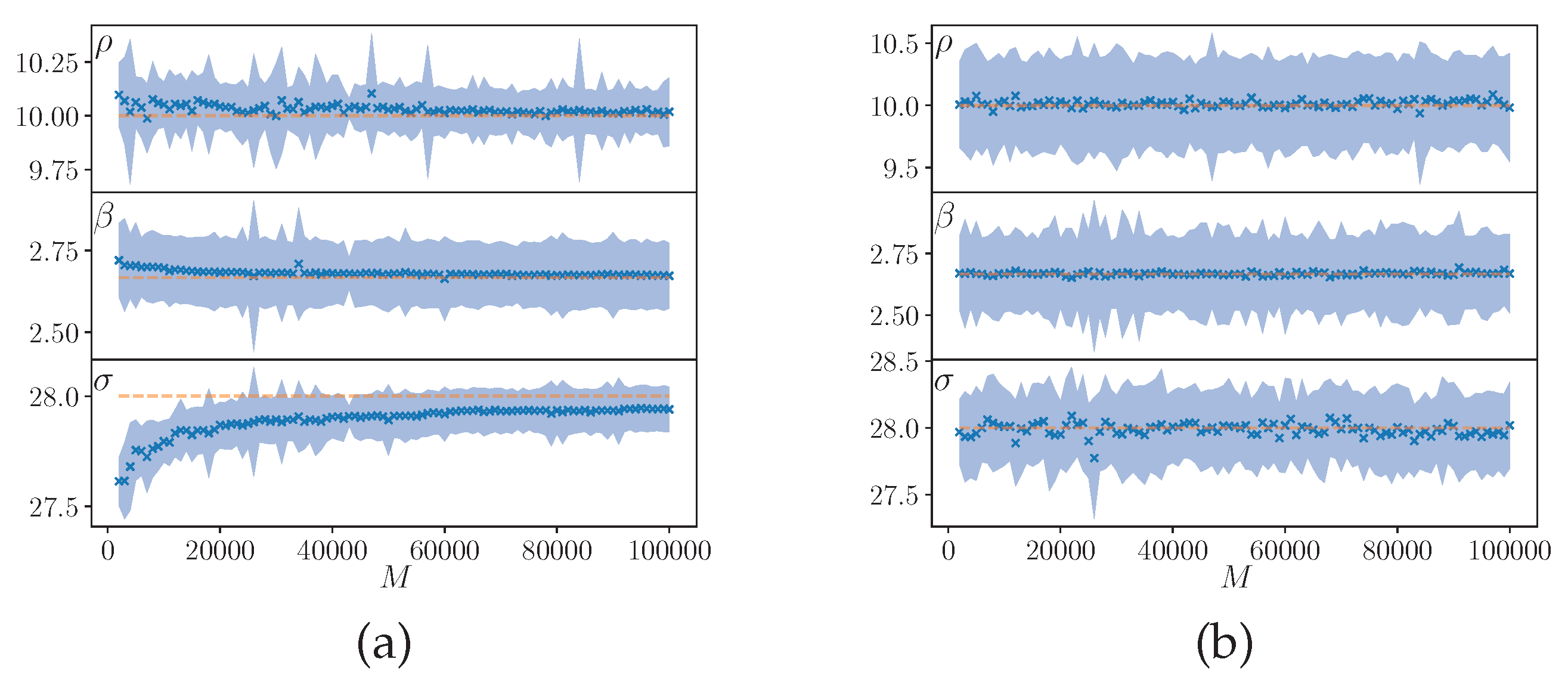
Without any a priori information about the true parameter values we randomly initialize the initial states and the parameters, so, using the cross-over operation can introduce a bias in the early stages of the optimization problem, as can be seen in Figure 9, where we compare the estimated parameters for different repetitions using an amplitude

δ = 0.8

with (Figure 9a) and without (Figure 9b) cross-over at every

t = T

. As the other simulations we randomly initialize the initial states and parameter values of the ensemble, we evolve the system, after the transient time

T_{T r a n s}

, up to

T = 100

with

d t = 0.01

and we suppose to be able to measure the x direction with

τ = 0.2

The cross-over allow to make jumps in the parameters space, but in the early stage of the optimization process these jumps can cause the ensemble convergence to wrong values. On the other hand, the cross-over can reduce the variance of the ensemble estimation, so it can help in the last steps, or for fine tuning. Future work is needed to explore more in details this option.

9. Conclusions

We have shown that it is possible to exploit several aspects of the master-slave synchronization to retrieve the parameters of the master system (assumed to be a real, physical one) though a simulated replica. In this way, it is also possible to perform measurements impossible on the real system, using the simulated replica.

We have extended the original Pecora-Carrol synchronization scheme [10], to partial and intermittent coupling.

We have shown that synchronization can be achieved when some of the state variables are available for direct measurement and that the parameters of the original systems can be reconstructed by synchronization using a simulated annealing approach,.

We have then shown that the synchronization method can be exploited to retrieve unknown parameters even when variables are accessible only through a scalar function, using a pruned-enriching ensemble approach, similar to genetic algorithms without cross-over, which is then introduced without remarkable improvements.

This works is only a first glimpse into a wide field. The proposed methods can be applied to other dynamical systems, and their limits are still to be precisely defined.

Other important questions concern the dimensionality of systems, since real systems are only exceptionally described by low-dimensional dynamical systems, and the influence of noise that always affect real-life measurements.

Author Contributions

Conceptualization, F.B.; methodology, F.B.; software, F.B. and M.B.; validation, M.B.; formal analysis, F.B.; investigation, F.B. and M.B.; writing—original draft preparation, F.B.; writing—review and editing, F.B. and M.B.; visualization, M.B.; supervision, F.B. All authors have read and agreed to the published version of the manuscript.

Funding

This research received no external funding.

Acknowledgments

We acknowledge useful discussions with Sara Beltrami.

Conflicts of Interest

The authors declare no conflict of interest. The authors had no role in the collection of data from Wikipedia.

Sample Availability

All codes are available upon request.

References

Lorenz, E. The Essence of Chaos (Jessie and John Danz Lectures), paperback ed.; University of Washington Press, 1995; p. 240.
Evensen, G.; Vossepoel, F.C.; van Leeuwen, P.J. Data Assimilation Fundamentals: A Unified Formulation of the State and Parameter Estimation Problem (Springer Textbooks in Earth Sciences, Geography and Environment), kindle edition ed.; Springer, 2022; p. 415.
Geer, A.J. Learning earth system models from observations: machine learning or data assimilation? Philosophical Transactions of the Royal Society A: Mathematical, Physical and Engineering Sciences 2021, 379. [Google Scholar] [CrossRef] [PubMed]
Bonavita, M.; Alan Geer, P.L.; Massart, S.; Chrust, M. Data assimilation or machine learning? ECMWF Newsletter Number 167 - Spring 2021 https://www.ecmwf.int/en/newsletter/167/meteorology/data-assimilation-or-machine-learning, 2021. [Accessed 13-Feb-2023].
Strogatz, S.H. Nonlinear Dynamics And Chaos: With Applications To Physics, Biology, Chemistry And Engineering (Studies in Nonlinearity), hardcover ed.; CRC Press, 1994; p. 512.
Pikovsky, A.; Rosenblum, M.; Kurths, J. Cambridge nonlinear science series: Synchronization: A universal concept in nonlinear sciences series number 12; Cambridge nonlinear science series; Cambridge University Press: Cambridge, England, 2003. [Google Scholar]
Bagnoli, F.; Rechtman, R. Synchronization and maximum Lyapunov exponents of cellular automata. Physical Review E 1999, 59, R1307–R1310. [Google Scholar] [CrossRef]
Lorenz, E.N. Deterministic Nonperiodic Flow. Journal of the Atmospheric Sciences 1963, 20, 130–141. [Google Scholar] [CrossRef]
Pecora, L.M.; Carroll, T.L. Synchronization in chaotic systems. Physical Review Letters 1990, 64, 821–824. [Google Scholar] [CrossRef] [PubMed]
Pecora, L.M.; Carroll, T.L. Synchronization of chaotic systems. Chaos: An Interdisciplinary Journal of Nonlinear Science 2015, 25, 097611. [Google Scholar] [CrossRef]
Rössler, O. An equation for continuous chaos. Physics Letters A 1976, 57, 397–398. [Google Scholar] [CrossRef]
Newcomb, R.; Sathyan, S. An RC op amp chaos generator. IEEE Transactions on Circuits and Systems 1983, 30, 54–56. [Google Scholar] [CrossRef]
May, R.M. Simple mathematical models with very complicated dynamics. Nature 1976, 261, 459–467. [Google Scholar] [CrossRef]
Rulkov, N.F.; Sushchik, M.M.; Tsimring, L.S.; Abarbanel, H.D.I. Generalized synchronization of chaos in directionally coupled chaotic systems. Physical Review E 1995, 51, 980–994. [Google Scholar] [CrossRef] [PubMed]
Kirkpatrick, S.; Gelatt, C.D.; Vecchi, M.P. Optimization by Simulated Annealing. Science 1983, 220, 671–680. [Google Scholar] [CrossRef] [PubMed]
Takens, F. Detecting strange attractors in turbulence. In Lecture Notes in Mathematics; Springer Berlin Heidelberg, 1981; pp. 366–381. [CrossRef]
Packard, N.H.; Crutchfield, J.P.; Farmer, J.D.; Shaw, R.S. Geometry from a Time Series. Physical Review Letters 1980, 45, 712–716. [Google Scholar] [CrossRef]
Rosenbluth, M.N.; Rosenbluth, A.W. Monte Carlo Calculation of the Average Extension of Molecular Chains. The Journal of Chemical Physics 1955, 23, 356–359. [Google Scholar] [CrossRef]
Grassberger, P. Pruned-enriched Rosenbluth method: Simulations of θ polymers of chain length up to 1 000 000. Physical Review E 1997, 56, 3682–3693. [Google Scholar] [CrossRef]
Mitchell, M. An introduction to genetic algorithms; MIT Press: London, England, 1996. [Google Scholar]

Figure 1. Conditional Lyapunov maximal exponent for different coupling directions.

C_{x} = [1, 0, 0]

C_{y} = [0, 1, 0]

C_{z} = [0, 0, 1]

. In the last one, in orange, we also show the distance d (normalized at it’s maximum value obtained in the simulation) between the master and slave state variables for different coupling strengths (see also Figure 2).

Figure 1. Conditional Lyapunov maximal exponent for different coupling directions.

C_{x} = [1, 0, 0]

C_{y} = [0, 1, 0]

C_{z} = [0, 0, 1]


( $C_{x}$ )	( $C_{y}$ )	( $C_{z}$ )

Figure 2. Asymptotic distance d as function of the coupling strength p for different coupling directions. From the left to the right:

C = [1, 1, 1]

C_{x} = [1, 0, 0]

C_{y} = [0, 1, 0]

Figure 2. Asymptotic distance d as function of the coupling strength p for different coupling directions. From the left to the right:

C = [1, 1, 1]

C_{x} = [1, 0, 0]

C_{y} = [0, 1, 0]

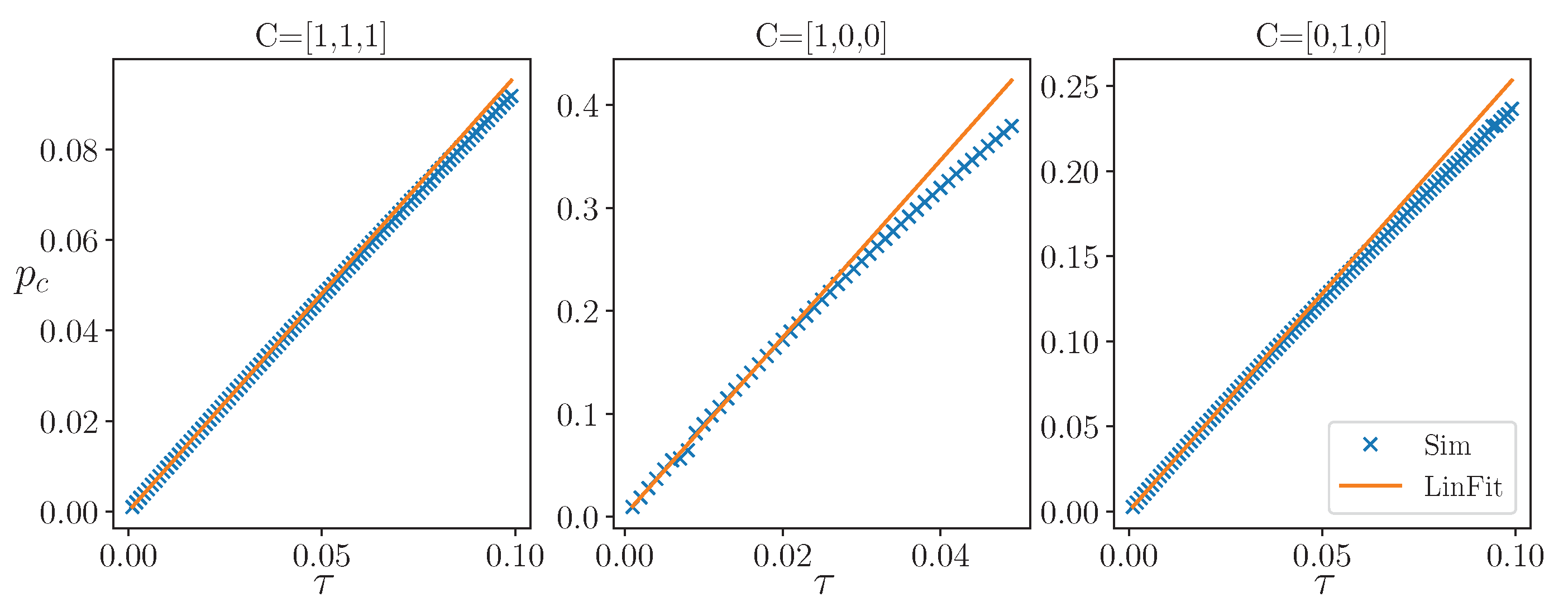
Figure 3. The dependence of the synchronization threshold on the intermittent parameter k such that

τ = k Δ t

for different coupling directions and it’s linear fit obtained using the first 20 time steps. The other parameters of the simulation are:

d t = 10^{- 3}

and

k_{m a x} = 50

for

C = [1, 0, 0]

k_{m a x} = 100

for the others.

Figure 3. The dependence of the synchronization threshold on the intermittent parameter k such that

τ = k Δ t

for different coupling directions and it’s linear fit obtained using the first 20 time steps. The other parameters of the simulation are:

d t = 10^{- 3}

and

k_{m a x} = 50

for

C = [1, 0, 0]

k_{m a x} = 100

for the others.

Figure 4. Heat map of the state-variable distance d for different values of parameter coupling

D = π D_{0}

(

0 \leq π \leq 1

) and state-variable coupling p for some state-variable coupling directions C and parameter coupling direction

χ

. (a)

C = [1, 1, 1]

χ = [1, 1, 1]

; (b)

C_{x} = [1, 0, 0]

χ = [1, 1, 1]

; (c)

C_{z} = [0, 0, 1]

χ = [1, 1, 1]

;. The line

π = 0

corresponds to Figure 2.

Figure 4. Heat map of the state-variable distance d for different values of parameter coupling

D = π D_{0}

(

0 \leq π \leq 1

) and state-variable coupling p for some state-variable coupling directions C and parameter coupling direction

χ

. (a)

C = [1, 1, 1]

χ = [1, 1, 1]

; (b)

C_{x} = [1, 0, 0]

χ = [1, 1, 1]

; (c)

C_{z} = [0, 0, 1]

χ = [1, 1, 1]

;. The line

π = 0

corresponds to Figure 2.


(a)	(b)	(c)

Figure 5. The state-variable distance d (dashed line) and parameter distance (color) as a function of temperature

θ

for

p = 0.6 ≫ p_{c}

and different coupling directions C. (a)

C = [1, 1, 1]

; (b)

C = [1, 0, 0]

; (c)

C = [0, 1, 0]

. We set

θ = 1

ϵ = 10^{- 4}

T = 100

Figure 5. The state-variable distance d (dashed line) and parameter distance (color) as a function of temperature

θ

for

p = 0.6 ≫ p_{c}

and different coupling directions C. (a)

C = [1, 1, 1]

; (b)

C = [1, 0, 0]

; (c)

C = [0, 1, 0]

. We set

θ = 1

ϵ = 10^{- 4}

T = 100


(a)	(b)	(c)

Figure 6. The schematic of the pruned-enriching method. The variation of the duplication of the nearer replicas is either on one of the state variables or one of parameters.

Figure 7. Parameters distance D at interval M for different amplitudes

δ

with (a)

Q_{i}

randomly initialized in the interval

(0.5, 30)

and (b)

Q_{i}

initialized near the “true” values

Q

by adding a random noise of amplitude

ϵ = 0.5

. (c) Variance of the distance D for different amplitudes

δ

for the last interval. The vertical lines indicate when the ensemble was restored to

t = 0

. The

Q_{i}

are initialized as in (a).

Figure 7. Parameters distance D at interval M for different amplitudes

δ

with (a)

Q_{i}

randomly initialized in the interval

(0.5, 30)

and (b)

Q_{i}

initialized near the “true” values

Q

by adding a random noise of amplitude

ϵ = 0.5

. (c) Variance of the distance D for different amplitudes

δ

for the last interval. The vertical lines indicate when the ensemble was restored to

t = 0

. The

Q_{i}

are initialized as in (a).


(a)	(b)	(c)

Figure 8. The distance between variable (black points, right axes) and parameters (left axes) as a function of time in the pruned-enriching method for 50 randomly selected replicas of the

h = 10000

used to estimated the parameters. We consider the situation where only measurement in coupling direction

C = [1, 0, 0]

are available at every

k = 20

temporal steps

d t

, so we embed our time series in an embedding space of dimension

d_{e} = 5

Figure 8. The distance between variable (black points, right axes) and parameters (left axes) as a function of time in the pruned-enriching method for 50 randomly selected replicas of the

h = 10000

used to estimated the parameters. We consider the situation where only measurement in coupling direction

C = [1, 0, 0]

are available at every

k = 20

temporal steps

d t

, so we embed our time series in an embedding space of dimension

d_{e} = 5

Figure 9. Estimation (x) and standard deviation (blue area) of the parameters computed using the first half of the ensemble with (a) and without (b) cross-over. The true values are also shown (dotted orange lines).


(a)	(b)

Table 1. Maximum conditional Lyapunov exponent estimated using the asymptotic distance

| d |

between Master and coupled Slave systems (

λ_{sim}

) and derived from linear fit (

λ_{fit}

Table 1. Maximum conditional Lyapunov exponent estimated using the asymptotic distance

| d |

between Master and coupled Slave systems (

λ_{sim}

) and derived from linear fit (

λ_{fit}

	$C = [1, 1, 1]$	$C_{x} = [1, 0, 0]$	$C_{y} = [0, 1, 0]$
$λ_{lin}$	$0.995$	$8.840$	$2.670$
$λ_{fit}$	$0.961$	$8.619$	$2.555$

Table 2. Estimated parameters obtained using the pruned-enriching algorithm with

δ

variable. On the last column we also show the variance on the ensemble members of the estimated parameters.

Table 2. Estimated parameters obtained using the pruned-enriching algorithm with

δ

variable. On the last column we also show the variance on the ensemble members of the estimated parameters.

	real	ens. mean	ens. variance
$σ$	$10.000000$	$9.997584$	$0.003873$
$β$	$2.666667$	$2.664959$	$0.001000$
$ρ$	$28.000000$	$28.017719$	$0.004583$

Disclaimer/Publisher’s Note: The statements, opinions and data contained in all publications are solely those of the individual author(s) and contributor(s) and not of MDPI and/or the editor(s). MDPI and/or the editor(s) disclaim responsibility for any injury to people or property resulting from any ideas, methods, instructions or products referred to in the content.

© 2023 by the authors. Licensee MDPI, Basel, Switzerland. This article is an open access article distributed under the terms and conditions of the Creative Commons Attribution (CC BY) license (http://creativecommons.org/licenses/by/4.0/).

Copyright: This open access article is published under a Creative Commons CC BY 4.0 license, which permit the free download, distribution, and reuse, provided that the author and preprint are cited in any reuse.

Alerts

MDPI Initiatives

Important Links

Choose an area of interest and we will send you notifications of new preprints at your preferred frequency.

Disclaimer

Synchronization, Control and Data Assimilation of the Lorenz System

Abstract

Keywords:

Subject:

1. Introduction

2. Pecora-Carrol synchronization

3. Conditional coupling

4. Partial conditional coupling

5. Intermittent synchronization

6. Generalized synchronization

7. Parameter estimation

8. Pruned-enriching approach

9. Conclusions

Author Contributions

Funding

Acknowledgments

Conflicts of Interest

Sample Availability

References

MDPI Initiatives

Important Links

Subscribe