Preprint
Article

Deep Convolutional Neural Network for Plume Rise Measurements in Industrial Environments

Altmetrics

Downloads

106

Views

26

Comments

0

A peer-reviewed article of this preprint also exists.

This version is not peer-reviewed

Submitted:

08 April 2023

Posted:

10 April 2023

You are already at the latest version

Alerts
Abstract
Estimating plume cloud height is essential for various applications, such as global climate models. Smokestack plume rise is the constant height at which the plume cloud is carried downwind as its momentum dissipates and the plume cloud and the ambient temperatures equalize. Although different parameterizations are used in most air-quality models to predict the plume rise, they have been unable to estimate it properly. This paper proposes a novel framework to monitor smokestack plume clouds and make long-term, real-time measurements of the plume rise. For this purpose, a three-stage framework is developed based on Deep Convolutional Neural Networks (DCNNs). In the first stage, an improved Mask R-CNN, called Deep Plume Rise Network (DPRNet), is applied to recognize the plume cloud. Then, image processing analysis and least squares theory are respectively used to detect the plume cloud’s boundaries and fit an asymptotic model into their centerlines. The y-component coordinate of this model’s critical point is considered the plume rise. In the last stage, a geometric transformation phase converts image measurements into real-life ones. A wide range of images with different atmospheric conditions, including day, night, and cloudy/foggy, have been selected for the DPRNet training algorithm. Obtained results show that the proposed method outperforms widely-used networks in smoke border detection and recognition.
Keywords: 
Subject: Environmental and Earth Sciences  -   Remote Sensing

1. Introduction

Smokestack Plume Cloud (PC) rises due to momentum and buoyancy. Finally, the PC dissipates and is carried downwind at a constant height. This height is called plume rise height or Plume Rise (PR). PR calculation is not straightforward, and it is a substantial problem in predicting the dispersion of different harmful effluents into the air [1]. PR contributes to 1) the distance pollutants carried downwind, 2) their concentration at the surface, where they are deposited in the green environment or inhaled by people, and 3) the amounts of greenhouse gases mixed into the upper troposphere. Therefore, accurate measurement of the PR is of concern for research and operational applications such as air-quality transport models, local environment assessment cases and global climate models [2].
The parameterizations of PR prediction were developed in the 1960s by Briggs [3,4]. Dimensional analysis was used to estimate the PR based on smokestack parameters and meteorological measurements in different atmospheric conditions. Early observations of PR were used to test and rectify the parameterizations developed using dimensional analysis [5]. Wind tunnel studies and field observations using technologies including film photography, theodolites, and cloud-height searchlights [6] were several calibration techniques utilized in this domain. There are also three-dimensional air-quality models using parameterization equations, including GEM-MACH [7], CAMx [8], and CMAQ [9].
Some studies tested the parameterizations of PR prediction in the 1970s and 1980s by comparing them to actual observations and demonstrated that the Briggs equations overestimate the PR [10,11,12,13]. In 1993, an aircraft-based measurement was done to measure SO 2 emissions of a power plant which indicated an overestimation of about 400 m [14]. Although these earlier studies showed some degree of overestimation, in 2002, Webster et al. [15] performed surface measurements and concluded that the Briggs parameterizations tend to underestimate PR. In 2013, as part of the Canada-Alberta Joint Oil Sands Monitoring (JOSM) Plan, an aerial measurement study was done in northern Alberta’s Athabasca oil sands region to study the dispersion and chemical processing of emitted pollutants [16,17,18]. The project consisted of 84 flight hours of an instrumented Convair aircraft over 21 flights designed to measure pollutants emissions, study the transformation of chemicals downwind of the industry, and verify satellite measurements of pollutants and greenhouse gases in the region. Using aircraft-based measurements and reported smokestack parameters and meteorological data, it was demonstrated that the Briggs equations significantly underestimate PR at this location.
Given the results of [16,17,18] and the gap of more than 30 years since the Briggs equations were developed and previously tested, there is a need for further testing and possible modification of the Briggs equations based on modern observation techniques. In recent decades, there have been many significant advancements in environmental monitoring activities over industrial regions for safety and pollution prevention [19,20,21,22]. Moreover, several smoke border detection and recognition models have been introduced recently using digital image analysis, such as wavelet and support vector machines [23], LBP and LBPV pyramids [24], multi-scale partitions with AdaBoost [25], and high-order local ternary patterns [26] which are well-performed and impressive. These improvements have led to the development of instrumentation which can be deployed near any smokestack to give information on pollutant dispersion and potential exposure to people downwind. This information will be based on actual real-time observation, i.e. digital images, as opposed to potentially erroneous and decades-old parameterizations. Due to the similarity of our work to smoke recognition on the one hand, and on the other, the unavailability of PC recognition research, smoke recognition studies will be reviewed in the following.
To find the smoke within an image or a video frame, either a rough location of smoke is identified using bounding boxes called smoke border detection [27], or pixels are identified and classified in detail, named smoke recognition [29]. Due to the translucent edges of smoke clouds, the recognition task needs far more accuracy than border detection. Traditional smoke recognition methods utilize manual features, which lead to low accuracy recognition results due to a large variety of smoke appearances. These low-level features consist of motion characteristic analysis of the smoke [30], smoke colour [31], and smoke shape [32]. In another research, [33] took advantage of the Gaussian Mixture Model (GMM) to detect the motion region of the smoke and [34] combined rough set and region growing methods as a smoke recognition algorithm which seems to be a time-consuming algorithm due to the computational burden of the region growing process. Since using colour information is less effective due to the similarity of smoke colour to its surrounding environment, the combination of motion and colour characteristics is considered for smoke recognition [35]. Some algorithms utilize infrared images and video frames in their experiments [36], which are not easily accessible and can increase the project’s costs. Moreover, using digital images makes the algorithm more flexible as it can be used with more hardware. On the other hand, some smokes are too close to the background temperature to be captured by the near red-channel wavelength. A higher-order dynamical system introduced in 2017 used particle swarm optimization for smoke pattern analysis [37]. However, this approach had a low border detection rate and high computational complexity.
In recent years, deep learning-based methods, especially Convolutional Neural Network (CNN) based methods, have led to significant results in semantic segmentation [38] and object recognition [39]. Similarly, these methods are widely used in smoke border detection and recognition [40] with different architectures such as three-layer CNN [41], generative adversarial network (GAN) [42], and two-path Fully Convolutional Network (FCN) [28]. Recently, a count prior embedding method was proposed for smoke recognition to extract information about the counts of different pixels (smoke and non-smoke) [43]. Experimental results showed an improvement in the recognition performance of these studies. However, the high computational complexities of these huge models are an obstacle to their use in PR real-time observations.
We have proposed a novel framework using Deep Convolutional Neural Network (DCNN) algorithms to measure PR. Our approach comprises three stages: 1) recognizing the PC region using an improved Mask R-CNN, 2) extracting the PC’s Neutral Buoyancy Point (NBP) from the centerline of the recognized PC, and 3) transforming the PC’s geometric measurement from an image-scale to real-world scale.
This strategy accurately recognizes the PC and measures PR in real-time. Here, we reinforce the bounding box loss function in Region Proposal Network (RPN) [46,47] through engaging a new regularization to the loss function. This regularizer restricts the search domain of RPN to the smokestack exit. In other words, it minimizes the distance between the proposed bounding boxes and the desired smokestack exit, called smokestack exit loss ( L S ). The proposed method is also computationally economical because it generates only a limited number of anchor boxes swarmed across the desired smokestack exit. Consequently, the main contributions of this paper can be summarized as follows:
  • Proposing Deep Plume Rise Network (DPRNet), a deep learning method for PR measurements, by incorporating PC recognition and image processing-based measurements. We have provided a reproducible algorithm to recognize PCs from RGB images accurately.
  • To the best of our knowledge, this paper estimates the PCs’ neutral buoyancy coordinates for the first time, which is of the essence in environmental studies. This online information can help update related criteria, such as the live air-quality health index (AQHI).
  • A pixel-level recognition dataset, Deep Plume Rise Dataset (DPRD), containing: 1) 2500 fine segments of PCs, 2) The upper and lower boundaries of PCs, 3) The image coordinates of smokestack exit, 4) The centerlines and NBP image coordinates of PCs, is presented. As is expected, the DPRD dataset includes one class, namely PC. Widely-used DCNN-based smoke recognition methods are employed to evaluate our dataset. Furthermore, this newly generated dataset was used for PR measurements.
This paper is organized as follows—Section 2 briefly explains the theoretical information used in our proposed framework. Section 3 describes our proposed framework for measuring the PR of a desired smokestack. Then, Section 4 present our dataset collection procedure, under-study site, experimental results of the proposed method and evaluation results using different metrics, and PR and PR distance calculations. Finally, this research’s conclusions, findings, and future studies are described in Section 5.

2. Theoretical background

2.1. Briggs PR prediction

The PR calculation is an ill-posed problem to predict the dispersion of harmful effluents in atmospheric science [1]. PR is affected by two phenomena, buoyancy and momentum. Typically, the PCs are buoyant, which means they are hotter than the ambient air. Therefore, they rise since they are less dense than the surrounding air. Also, the PCs have a vertical velocity and momentum when they exit the smokestack, which causes them to rise again. PCs can also fall due to the gravitational force when cold and dense and when some surrounding obstacles cause them to move downwind [48]. In 1975 Briggs proposed an equation for the maximum distance of the PR, which was practically suitable for calculating PR. Considering both momentum and buoyancy in calculations, PR ( Δ z ) in horizontal distance x from the smokestack exit can be obtained as [4],
Δ z = ( 3 F m x 0 . 6 2 u ¯ 2 + 3 F b x 2 2 × 0.6 2 u ¯ 3 ) 1 / 3
where 0.6 is an entrainment rate (the mean rate of increase of PC in the wind direction) and u ¯ is the mean horizontal wind speed. Also, the momentum flux parameter ( F m ) and buoyancy flux parameter ( F b ) are defined below,
F m = [ ρ s ¯ ρ ¯ ] r s 2 w s ¯ 2
F b = [ 1 ρ s ¯ ρ ¯ ] g r s 2 w s ¯ 2
where ρ s ¯ is the smokestack gas density, ρ ¯ is the atmospheric air density, r s is the smokestack radius, w s ¯ is the vertical velocity of the smokestack gas, and g is the acceleration due to gravity.
It should be noted that if we evaluate the wind speed at the local PC height and not the source height, the calculations should be operated iteratively [49,50]. The wind strongly affects PC buoyancy, horizontal momentum movements, and PR [1]. Moreover, PR is unaffected by wind speed fluctuations in stable conditions with low turbulence, making the measurements difficult. However, significant PR variations in unstable conditions have been witnessed at a fixed distance downwind.

2.2. CNN and convolutional layer

CNNs are particular types of neural networks suitable for processing grid data, such as image data with a two-dimensional or three-dimensional mesh structure of pixels. The name given to a CNN is derived from the convolutional layers used in it. Each convolutional layer contains several kernels and biases that are locally applied to the input and produces a feature map or an activation map according to the number of filters. Suppose this convolutional layer is applied to the input image in a two-dimensional manner. In that case, its j t h feature map O j , which is obtained by using the j t h kernel, is calculated at the position ( x , y ) as [51],
O j x y = B j + k m = 0 M 1 n = 0 N 1 w j m n z k ( x + m ) ( y + n )
where k moves along the depth dimension of input z R p × q × r and w j m n is the two-dimensional kernel weight W R M × N at position ( m , n ) . B j is the bias matrix.

2.3. Mask R-CNN

Mask R-CNN is a region-based CNN family member proposed in [44] and is used widely in different identification tasks, including COCO dataset recognition. Firstly, RCNN was presented in [52], where computer vision techniques generated region proposals. Then in [47], Fast RCNN was introduced with a CNN before region proposals to reduce running time. In 2017, Faster RCNN continued this evolution and offered the RPN to propose regions of interest (ROIs) [53]. Finally, Mask R-CNN, as an extension of Faster RCNN, added a CNN for pixel-level recognition of the border-detected objects. Mask R-CNN is a relatively simple model and easy to generalize to other similar tasks [44]. Therefore, Mask R-CNN can create pixel-level masks for the objects besides object localization and classification tasks.

2.3.1. RPN

An RPN is a deep FCN that proposes regions and is crucial to the Mask R-CNN. RPN helps selectively focus on valuable aspects within the input images. This network takes an image and gives a set of region proposals beside their scores for being an object. It slides a window over the convolutional feature map (backbone output) and maps it to a lower-dimensional feature. The generated feature is then fed into two fully-connected layers to obtain the proposed regions class (object vs. non-object) and four corresponding coordinates [53]. A maximum of k possible proposals are parameterized relative to k reference boxes or anchors for each sliding window location. RPN is trained end-to-end by back-propagation and stochastic gradient descent. Figure 1 depicts a scheme of RPN in which the proposed regions are generated as the module outputs.

2.3.2. Loss function

Mask R-CNN loss function is a weighted summation of other losses related to different sections of this comprehensive model. As a definition based on [44], a multi-task loss function is proposed on each sampled ROI as,
L = L c l s + L r e g + L m s k
where L c l s recognizes the class type of each object while L r e g attempts to find the optimum anchor box for each object. Note that, in this study, we have one class, PC. L m s k tries to recognize the optimum object’s segment in each bounding box.

3. Methodology

The proposed framework for PR measurement is represented in Figure 2. The images containing PC(s) are fed to DPRNet for PC border detection and recognition. PR and PR distance are then measured on DPRNet’s output based on extracting the NBP. The measured image coordinates of NBP are combined with the wind direction information to be processed by geometric transformation calculations. The main output of the system will reveal the PR as a physical height and the PR distance downwind at which the PR occurs. Also, a schematic diagram in Figure 6 describes the definitions of PC centerline, PR and PR distance.

3.1. DPRNet

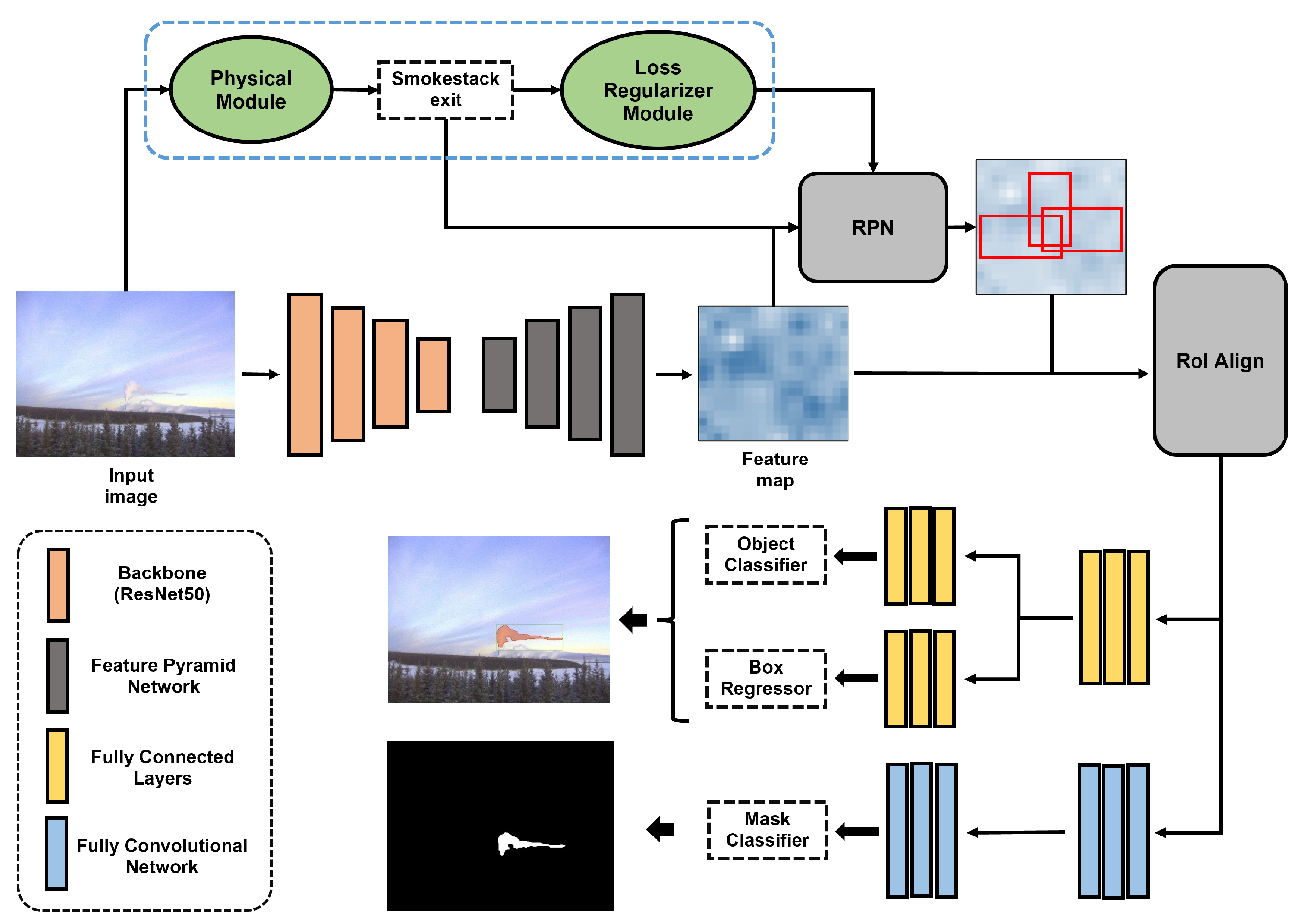
This research aims to precisely recognize the PC of the desired smokestack from a wide range of image datasets captured from the study area. DPRNet is an adapted Mask R-CNN version with two novel smokestack PR measurement modules. These modules are 1) the physical module and 2) the loss regularizer module. These modules can improve RPN performance in locating the most probable proposal PCs. Mask R-CNN is the base of our proposed method, one of the widespread border detection and recognition methods. This robust framework can consider the irregular shapes of the PC, its translucent edges, and similar pixel values of the PC to its background [44]. As seen in Figure 3, DPRNet is an application-oriented version of Mask R-CNN to which two new modules have been added.
In this architecture, ResNet50 [54] is used as the backbone network to extract feature maps of the input images. Feature Pyramid Network (FPN) uses all these feature maps to generate multi-scale feature maps, which carry more helpful information than the regular feature pyramid. Then, RPN detects the PC by sliding a window over these feature maps to predict whether there is a PC and locate the existing PC by creating bounding boxes. Therefore, we have a set of PC proposals from RPN and the generated feature map by the backbone network. The ROI Align module works to scale the proposals to the feature map level and prevent misalignment by standardizing the aspect ratios of the proposals. Finally, these refined feature maps are sent to three different outputs. The first is a classification block that decides whether the ROI corresponds to the foreground (PC). The second one is a regression block which predicts the bounding boxes based on the provided ground truth. And the last block indicates a recognition mask for the detected PC using an FCN [55].
Two modules are added to Mask R-CNN to improve its efficiency and reduce the computational burden. The first module, a simple image processing one, approximates smokestack. The second module attempts to improve the loss related to L r e g by adding a regularizer loss, elaborated in Section 3.1.2. These modules are explained in detail in the following subsections.

3.1.1. Physical module

The physical module was implemented to detect an exit point where the PC of interest rises from a chimney stack in the middle of the imagery. Please note that this module is only used during the training phase, and the exit point is automatically predicted in the network’s inference process without the physical module. In this physical module, the smokestack exit is detected from ground truth binary image by an image processing technique detecting extrema points of foreground boundaries [57]. It stands to reason that the smokestack exit is the feasible region of the plume rise. As a result, proposed regions can be considered around this point (Figure 3). Thanks to this module, the method does not detect small PC pieces, sometimes seen in different parts of images other than the smokestack exit.
To extract the smokestack exit, eight extrema points on each PC’s boundary are extracted based on image processing analysis [57], illustrated in Figure 4. This algorithm first smoothes noises of foreground regions (i.e., PC region labelled in the ground truth imagery). After that, it tracks boundary pixels of the foreground region and extracts eight extrema points showing the locally highest geometric curvature. Each PC segment’s bottom-left corner is considered a smokestack exit.

3.1.2. Loss regularizer module

Based on Section 2.3.2, it is a crucial problem to set an efficient loss function, which can make the model stable as it can get. In this regard, a new regularizer is added to the loss function, which regresses the coordinates of the most attainable PC regions. Indeed, we try to minimize the distance of proposed bounding boxes by RPN and the smokestack exit. Suppose a box with coordinates of ( x , y , w , h ) is defined here. In that case, the regression loss related to the smokestack exit can be defined as,
L S = R ( u u * ) ,
in which,
u x = x x a w a , u y = y y a h a , u w = log ( w w a ) , u h = log ( h h a ) , u x * = x * x a w a , u y * = y * y a h a , u w * = log ( w * w a ) , u h * = log ( h * h a )
where u and u * represent the coordinates of our predicted and ground truth smokestack exit and R is the robust loss function. Note that subscript a and superscript * variables represent the anchor coordinate and the ground truth coordinates, respectively, while the rest are defined as the predicted coordinates. The point ( x , y ) indicates the position of the bounding box’s top-left corner and the parameters w and h are, respectively, the width and height of the bounding box.
Unlike the Mask R-CNN model, in DPRNet, the loss regularizer module ( L S ) minimizes the recognition task errors of a specific PC, which copes with the main problems of this model, such as missing the desired smokestack exit and multi-box proposal for a single PC. L S helps us avoid spanning the whole image pixels, causing high training time and computational complexities.

3.2. NBP extraction

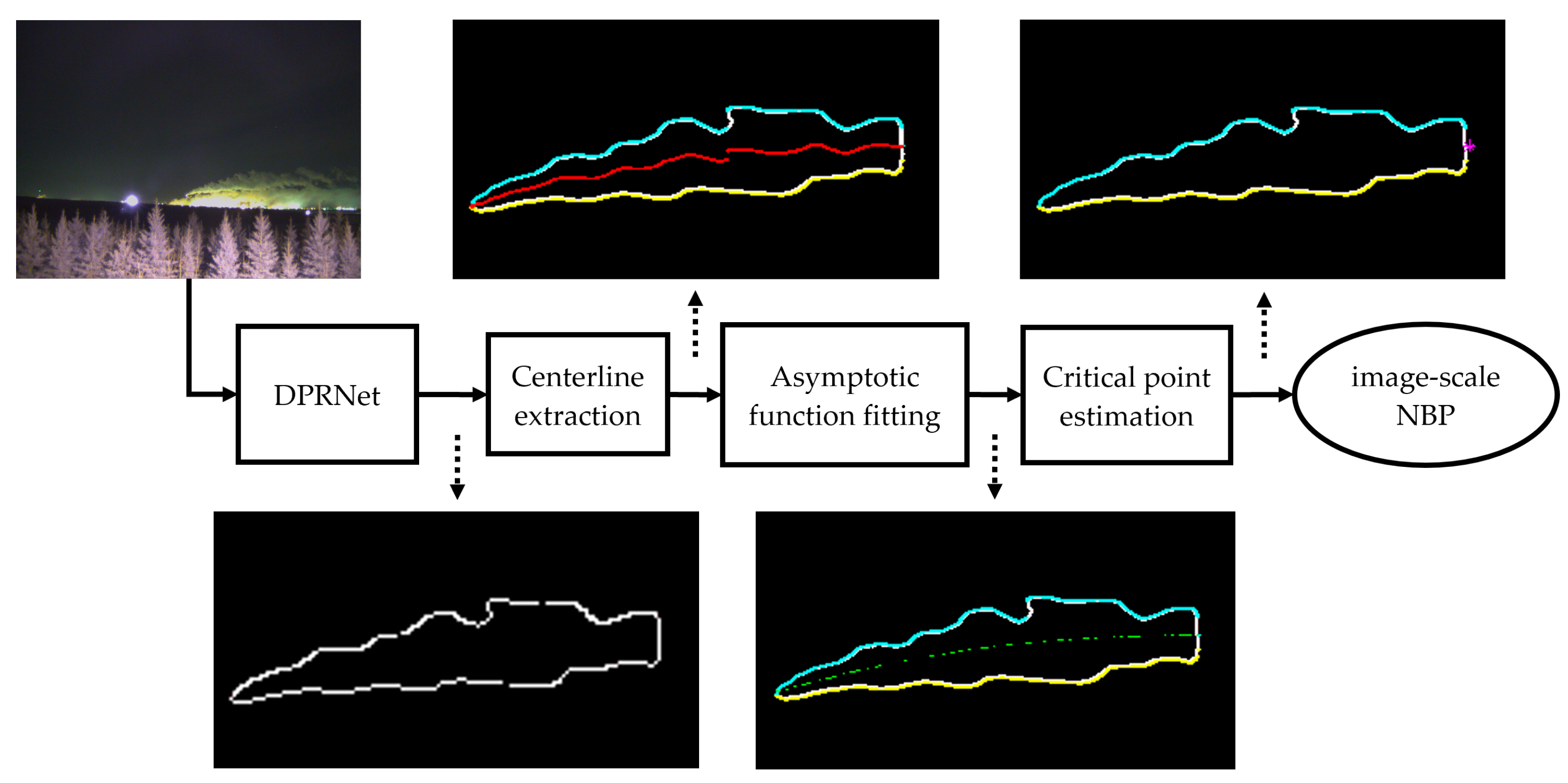
As seen in Figure 2, the PR measurements are performed based on the extraction of NBP for every PC image. The NBP extraction phase can be summarized in three steps. An overall processing chain is shown in Figure 5. Firstly, the centerline is extracted as the PC’s skeletonized curve., which consists of some points demonstrating the meandering of the PC. To accomplish this task, we classify the PC’s boundary pixels into upper and lower boundary pixels, represented with cyan and yellow coloured lines, respectively, in Figure 5. This binary classification of boundary lines is conducted by tracking the upper pixel, found at the highest row index, while the lowest one for the lower boundary pixel from each fixed column index with the coordinate origin at the lower-left corner in the image space. The center line pixel per each column is found by simply averaging the two-row indices. Measuring the NBP for plume rise in the context of atmospheric science using imagery requires identifying the point at which the buoyant force from the plume is equal to the gravitational force acting on it. At this point, the plume ceases to rise further and begins to spread laterally. The central lines detected from the imagery show salient visual cues caused by many factors involved in atmospheric dynamics. However, they cannot explicitly estimate the NBP and require a physical interpretation to determine the NBP from the centerlines. Thus, we fit an asymptotic function [59] to the center line pixels using a conventional least-squared method to drive this function’s horizontal asymptote to determine the NBP from the imagery. Equation 8 shows the asymptotic function employed in this study.
y = a e b x ; a , b > 0

3.3. Geometric transformation

To convert the image measurement results to real-world ones, we need to perform some calculations to transform the PR ( Δ z ) and the PR distance ( X m a x ) on an image to real-life measurements using wind direction.
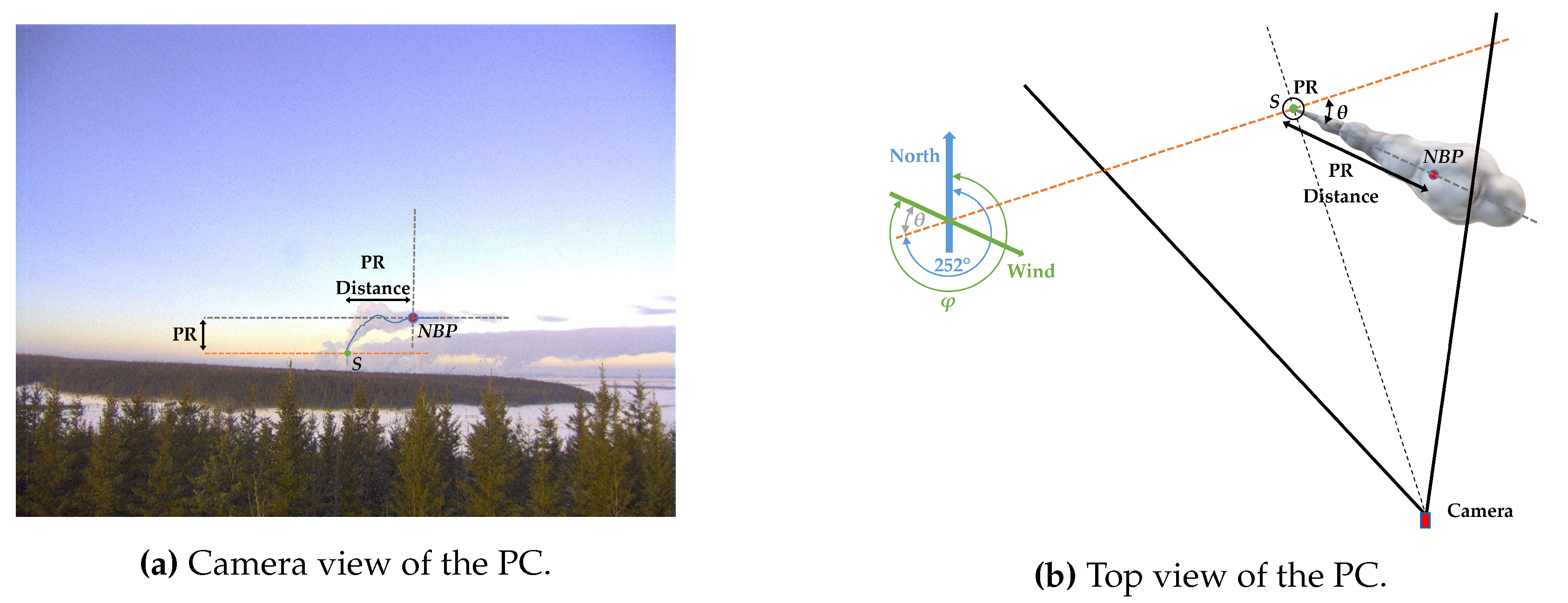
The PR distance can be defined as the horizontal distance between the smokestack exit and NBP, discussed in Section 3. Figure 6 shows PR and PR distance definitions on a sample PC image.
Figure 6. PR, PR distance, and N B P on a sample image. θ represents the PC deviation due to the wind, and φ denotes the wind direction. Also, S indicates the smokestack exit, and the blue line shows the PC centerline.
Preprints 70704 g006
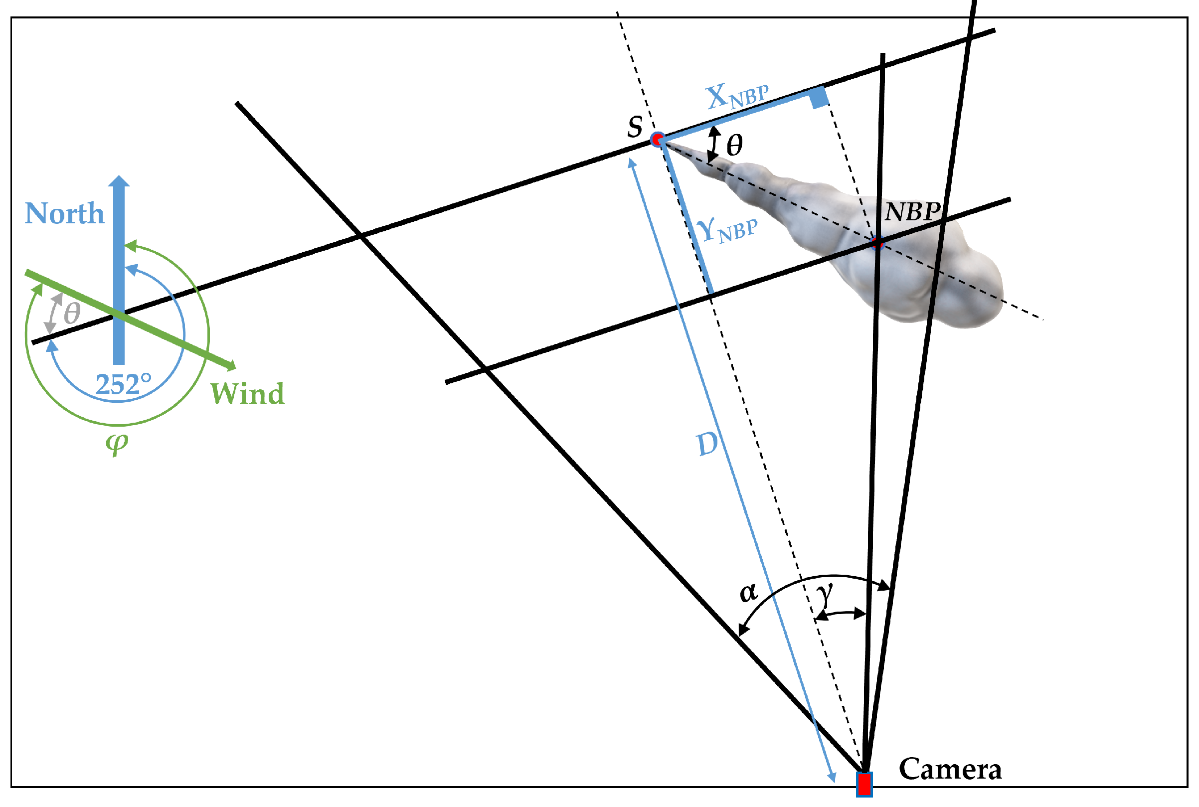
As observed in Figure 7 and Figure 8, the PC is affected by wind direction and is out of the image plane. Wind direction is always reported as degrees from the north, represented by φ . For instance, φ = 90 is wind from the east, and φ = 180 is wind from the south. Based on the camera’s position, capturing desired smokestack images, and geographical directions, wind direction relative to the image plane can be obtained as θ = | φ 252 | in this study (This information is prior knowledge). Accordingly, X N B P , shown in Figure 7, can be calculated by the following equation,
X N B P = D tan θ + 1 tan γ if θ 0 D 1 tan γ tan θ otherwise
where γ and θ are additional parameters that help us define equations as concisely as we can get. D indicates the distance between the camera and the smokestack.
We define G and G N B P as the value of the ground sample distance, respectively, at the image plane and the location of NBP. Consequently, based on [45],
G N B P = X N B P x N B P Z N B P = G N B P × z N B P Z S = G × z S
where Z S and z S are the distance between the smokestack exit and the image center, respectively, in real life and on the image.
Thus, the PR and the PR distance for each PC can be calculated as,
Δ z = | Z N B P | | Z S | , if | Z N B P | | Z S | | Z S | | Z N B P | , otherwise
X m a x = X N B P 2 + Y N B P 2

4. Experimental results and discussion

In this section, we describe our image datasets and the industrial area in which these image datasets have been collected and shared. Also, we will explain the validation metrics used to compare our proposed method with the other competitive methods in smoke border detection and recognition. Then, our discussion falls into two last sections, named comparison with existing smoke recognition methods and plume rise measurement, in which the performance of the proposed method is evaluated, and the PR is calculated based on our "DPRNet," respectively. To validate the performance of our proposed method, we used a computer equipped with Core i9, 3.70 GHz/4.90 GHz, 20 MB cache CPU, 64GB RAM and NVIDIA GeForce RTX 3080,10 GB graphic card. The total training time of the network was about one hour using Python 3.8 with PyTorch Deep Learning framework. Finally, for the geometric transformation and image processing analysis, we used MATLAB R2022b software.

4.1. Site description

The imaging system was deployed on a meteorological tower with a clear sightline to the desired smokestack operated by the Wood Buffalo Environment Association (WBEA). It is located outside the Syncrude oil sands processing facility north of Fort McMurray, Alberta, Canada. Figure 9 represents the satellite images, the location of the camera, and the desired smokestack.
WBEA operates a 10-meter-tall meteorological tower with a clear sightline to the smokestack at Syncrude (https://wbea.org/stations/buffalo-viewpoint). The camera system is mounted on this tower above the tree canopy because they are on a hill sloped downward from the tower location, and the biggest smokestack and its PC are always visible. The system consists of a digital camera with shutter control and a camera housing for weather protection with interior heating for window defrost and de-icing.
The Syncrude processing facility has six main smokestacks. The tallest one is about 183 m, and the heights of the other five are between 31 m to 76 m. To isolate a single smoke plume rise, we have concentrated on the area’s tallest one, which can help find the PR for one plume source. All six smokestacks are listed in Table 1. Wind directions during the capturing period were determined from the Mildred Lake Air Monitoring Station (https://wbea.org/stations/mildred-lake), located at the Mildred Lake airstrip (AMS02: Latitude: 57 . 05 , Longitude: 111 . 56 ), approximately 5 km from the Syncrude facility.

4.2. Deep Plume Rise Dataset (DPRD)

The greatest challenge in using deep learning for PC recognition is inadequate annotated images for training. Hence, creating image datasets for PC recognition for research and industry purposes is invaluable. For this study, 96 images were captured daily; for the first part of the project, 35K images were collected from January 2019 to December 2019. The collected images demonstrated various types of plume shapes in different atmospheric conditions. The dataset has been classified into day, night, and cloudy/foggy conditions. The collected dataset revealed that among 96 images captured daily, we have 48-day and 48-night images. There were some outlier images for different reasons, such as camera handle shaking, auto-focus problems, disturbing smoke and severe snow and hail. Furthermore, some PCs could not be recognized from their background, even by visual image inspection. As a consequence, among 35K collected images, 10684 were valid. Note that about 8110 images were captured when the facility was not working.
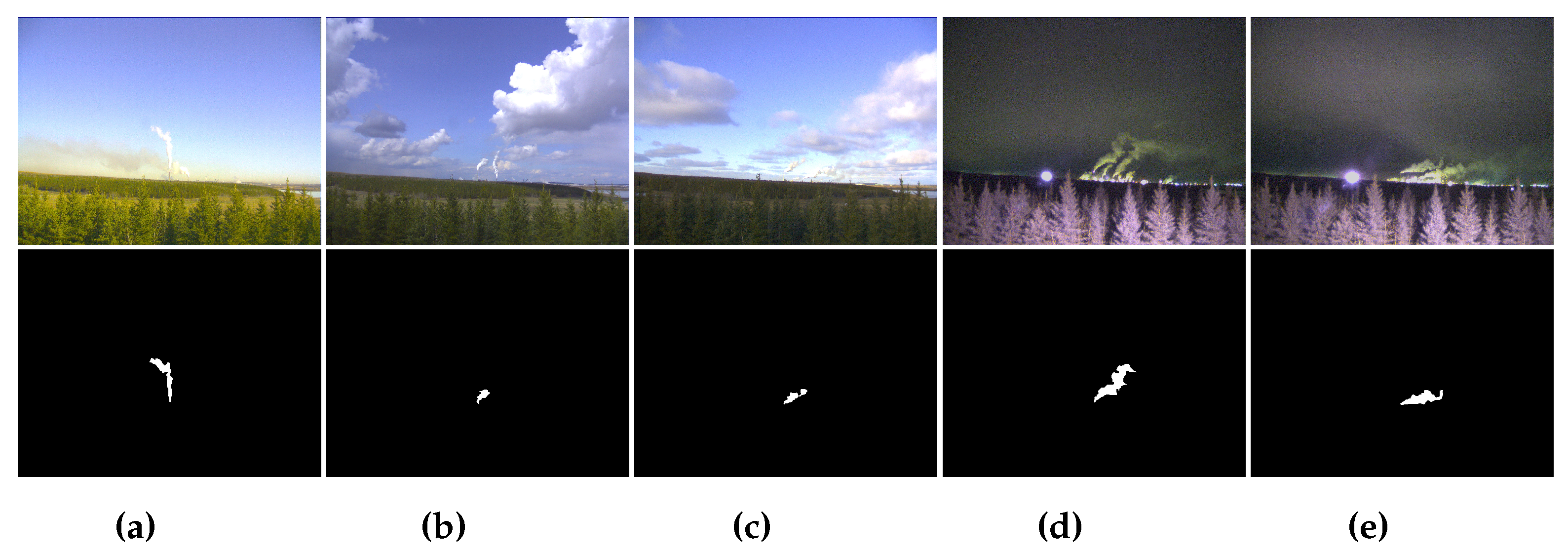
This paper introduces a new benchmark, DPRD, including a 2500 annotated dataset. DPRD contains PC upper and lower borders, smokestack exit image coordinates, PC centerline, and NBP image coordinates. 60% of DPRD is considered training data and 40% is used for validation and testing. Rows (a) and (b) in Figure 10 show sample images from the region and their corresponding ground truth, which are generated by the "Labelme" graphical image annotation tool at https://github.com/wkentaro/labelme. We tried to select images of different atmospheric conditions, such as clear daytime, nighttime, cloudy, and foggy, to represent the results of different situations.

4.3. Model validation metrics

The performance of the methods in question is evaluated using the metrics of accuracy, recall, precision and F1 score. These metrics are defined using four values of True Positive (TP), True Negative (TN), False Positive (FP), and False Negative (FN) obtained from the confusion matrix of each introduced method [58]. The accuracy validation metric is the ratio of observations predicted correctly to the total observations. In our application, the model’s accuracy represents how accurately our model can recognize the PC pixels. This criterion is valid as long as the values of FP and FN are almost the same [58]. Otherwise, other validation metrics should be considered. The foreground pixel coverage of the sample images is revealed in Figure 10, confirming that accuracy is not suitable for this study. Recall or sensitivity is the ratio of positive observations predicted correctly to all actual observations. Recall shows how many PC pixels are labelled among all the actual PC pixels. The recall is obtained as follows,
R e c a l l = T P T P + F N
Precision is the ratio of positive observations which are predicted correctly to all observations which are predicted as positive. This metric represents how many PC pixels exist among all the pixels labelled as PC. Therefore, a low rate of FP can achieve high precision. This validation metric is obtained as follows,
P r e c i s i o n = T P T P + F P
As it is implied from Equations 13 and 14, precision and recall take either FP or FN into account. The last validation measure in this paper, the F1 score, considers both FP and FN as a weighted average of recall and precision metrics. Unlike accuracy, this metric is more useful when FP and FN are not the same as in our study. Our FP is less than FN, or the amount of non-actual PC pixels predicted as PC pixels is less than that of actual PC pixels predicted as non-PC pixels. Therefore, the F1 score helps us look at both recall and precision validation metrics as follows,
F 1 s c o r e = 2 × R e c a l l × P r e c i s i o n R e c a l l + P r e c i s i o n

4.4. Comparison with existing smoke recognition methods

In this section, we evaluate the performance of DPRNet and compare it with several competitors. To choose suitable smoke recognition methods for comparison, we considered both the identification accuracy and computational complexity of the reviewed approaches, which led to the selection of DeepLabv3+ [56], FCN [55], and regular Mask R-CNN. Our proposed DPRNet is evaluated using three metrics introduced in Section 4.3.
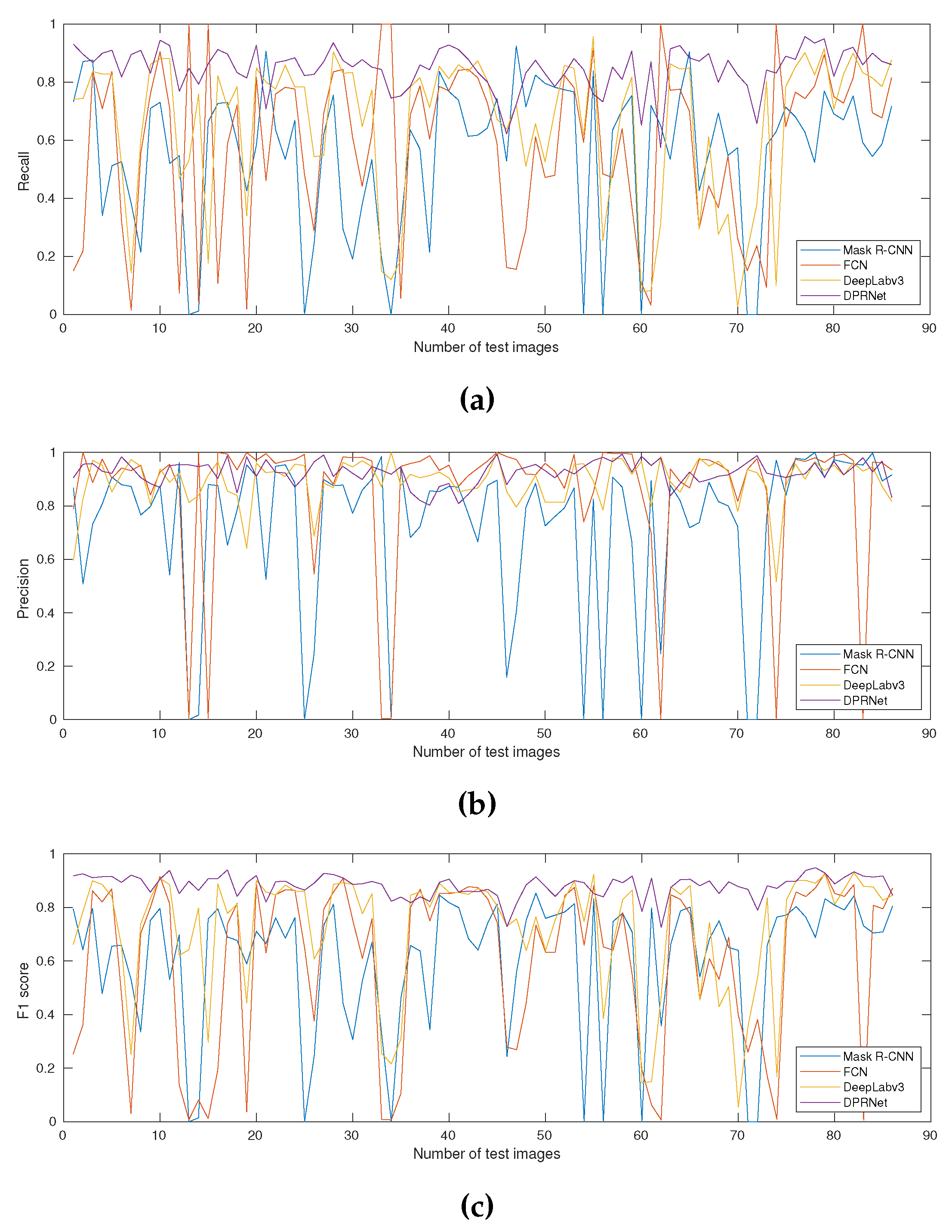
As is clear from Table 2, DPRNet performs much better than competitive methods for 90 test images selected from various day, night, foggy, and cloudy conditions. In detail, the recall and precision metrics express the reasonable difference between the models, which shows the effectiveness of the proposed model in recognizing the actual PC pixels. Compared to the rivals, the more considerable value of the F1 score guarantees that DPRNet outperforms the other three methods and shows the efficacy of this method. Among our competitive methods, DeepLabv3 performed better regarding all validation metrics, and Mask R-CNN had the worst performance.
Besides these average values, the detailed statistics for each model are given in Figure 11 in terms of each used validation metric. At a glance, our proposed method shows the most robustness in all circumstances. Of competitors, Mask R-CNN and FCN have the worst performance, whereas, DeepLabv3 has the best efficiency slightly.
To further validate our DPRNet performance, we compared the models over the day, night and foggy & cloudy data sets in terms of different validation metrics, which are given in Figure 12. It can be observed that all methods, except Mask R-CNN, have acceptable performance using day and night datasets. Even with night precision, FCN is better than our proposed method. However, as discussed in Section 4.3, this metric can only partially convey the merit of a model individually, and it needs to be analyzed with the F1 score. Our proposed DPRNet outperforms the other rival methods by recognizing roughly all of the PC pixels correctly. Most datasets are related to cloudy and foggy conditions and are frequently seen within image batches. The strength of our DPRNet is its robust performance in this case, which is of paramount importance in our application. The DPRNet could improve the recall metric by 66%, 58%, and 87% on average in cloudy and foggy conditions relative to FCN, DeepLabv3, and Mask R-CNN frameworks, respectively, which means that the proposed method is able to find the PC regions appropriately, using L S . This capability produces high-quality image recognition with a more complicated mixture of PCs and the sky behind. These high recall values help us meet our research application requirement, in which we should identify the entire PC stream for PR distance measurement.
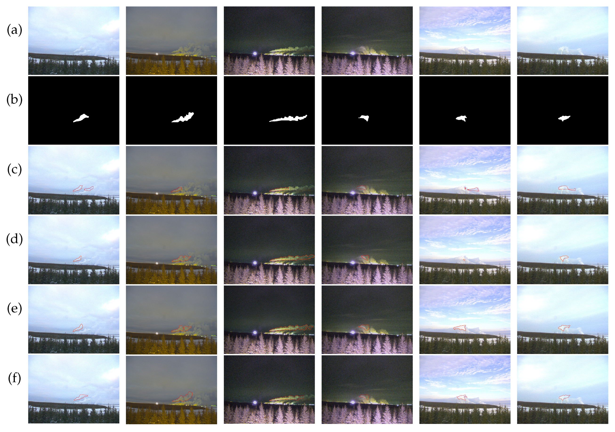
To demonstrate the qualitative results of the proposed method, we show some visual results to compare competitive methods. Figure 13 depicts these recognition results. The first two rows represent the input images and their corresponding ground truths, respectively, and the other rows give the output of different models. We tried to visualize samples from all classes such that the first two images are related to cloudy/foggy conditions, the second two are from the nighttime dataset, and the last two are obtained from our daytime dataset. It is observed that DPRNet outperformed the other methods by attaining high accuracy of PC localization and, consequently, correctly recognizing the desired smokestack PC.

4.5. Plume rise measurement

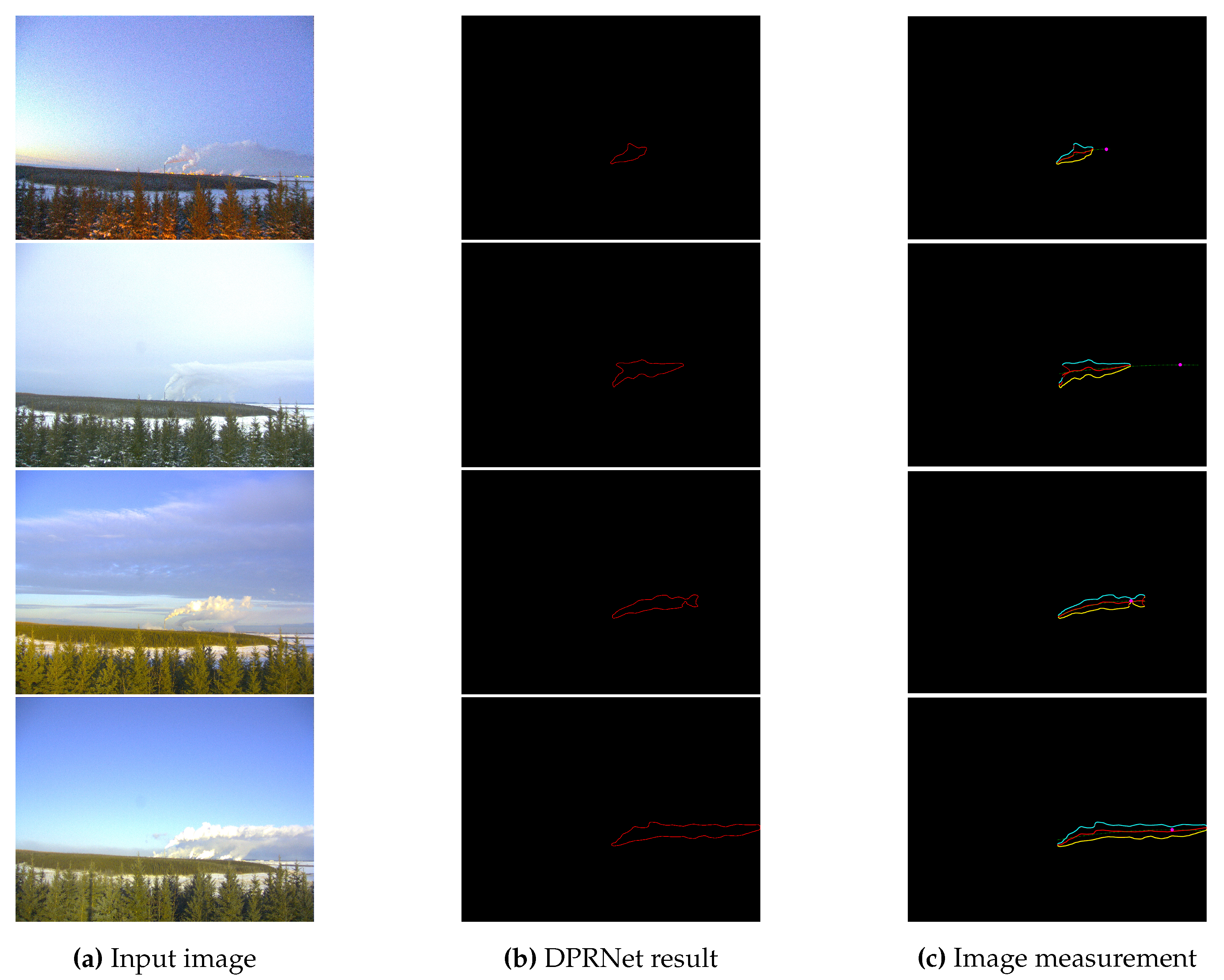
As discussed in Section 3, DPRNet gives PC border detection and recognition. Then, we take advantage of the NBP image coordinates and the wind direction information from the meteorological tower to obtain PR real-life measurements through geometric transformations. Figure 14 illustrates the asymptotic curve for four PC images and the automatically chosen point NBP, where the PC reaches neutral buoyancy. Apart from the PR and PR distance values of each sample PC, estimated by the proposed framework (tabulated in Table 3), the averaged hourly measured wind directions at the image sampling times are given as prior information of this study. These realistic PR and PR distance values within an extended period are required for future studies.

5. Conclusion

To measure the PR through remote sensing images, PC recognition is of the essence as the first step. In this regard, a novel deep learning-based method, inspired by the nature of the problem, is proposed in this paper to detect and recognize the PC accurately. In the next stage, image processing analysis is leveraged to extract the PC centerline. Afterward, the critical point of this curve is estimated, the y-component coordinate of which is equivalent to PR. Lastly, this image measurement is transformed into a real-life world under the geometric transformation stage. Experimental results indicate that the proposed method, DPRNet, significantly outperformed its rivals. This work also demonstrated that PR could be determined with a single-camera system and wind direction measurements, allowing further investigation and understanding of the physics of how buoyant PCs interact with their environment under different meteorological conditions. The proposed strategy can be extended to a more comprehensive method through several advancements in future research:
  • Generalizing DPRNet to predict the PC and PC centerline simultaneously.
  • Reinforcing DPRNet to recognize multi-source PCs occurring in industrial environments.
  • Conducting comparative studies using meteorological and smokestack measurements between the estimated PR and PR distance from the proposed framework and the Briggs parameterizations equations.
  • Briggs parameterization modification via estimated PR and PR distance from the proposed framework.

Acknowledgments

We want to acknowledge Wood Buffalo Environmental Association (WBEA) for assistance with the camera installation and maintenance at the air-quality monitoring site in the Syncrude facility in northern Alberta, Canada. The project is funded by the "Lassonde School of Engineering Strategic Research Priority Plan" and "Lassonde School of Engineering Innovation Fund," York University, Canada, and "Natural Sciences and Engineering Research Council of Canada – NSERC (grant no. RGPIN 2015-04292 and RGPIN 2020-07144)."

References

  1. G. A. Briggs, “Plume rise predictions,” in Lectures on air pollution and environmental impact analyses, pp. 59–111, Springer, 1982.
  2. K. Ashrafi, A. A. Orkomi, and M. S. Motlagh, “Direct effect of atmospheric turbulence on plume rise in a neutral atmosphere,” Atmospheric Pollution Research, vol. 8, no. 4, pp. 640–651, 2017.
  3. G. A. Briggs, “Plume rise: A critical survey.,” tech. rep., Air Resources Atmospheric Turbulence and Diffusion Lab., Oak Ridge, Tenn., 1969.
  4. G. Briggs, “Plume rise predictions, lectures on air pollution and environment impact analysis,” Am. Meteorol. Soc., Boston, USA, vol. 10, p. 510, 1975.
  5. J. Bieser, A. Aulinger, V. Matthias, M. Quante, and H. D. Van Der Gon, “Vertical emission profiles for europe based on plume rise calculations,” Environmental Pollution, vol. 159, no. 10, pp. 2935–2946, 2011.
  6. B. Bringfelt, “Plume rise measurements at industrial chimneys,” Atmospheric Environment (1967), vol. 2, no. 6, pp. 575–598, 1968.
  7. P. Makar, W. Gong, J. Milbrandt, C. Hogrefe, Y. Zhang, G. Curci, R. Žabkar, U. Im, A. Balzarini, R. Baró, et al., “Feedbacks between air pollution and weather, part 1: Effects on weather,” Atmospheric Environment, vol. 115, pp. 442–469, 2015.
  8. C. Emery, J. Jung, and G. Yarwood, “Implementation of an alternative plume rise methodology in camx,” Novato, CA, 2010.
  9. D. Byun, “Science algorithms of the epa models-3 community multiscale air quality (cmaq) modeling system,” EPA/600/R-99/030, 1999.
  10. B. E. Rittmann, “Application of two-thirds law to plume rise from industrial-sized sources,” Atmospheric Environment (1967), vol. 16, no. 11, pp. 2575–2579, 1982.
  11. W. G. England, L. H. Teuscher, and R. B. Snyder, “A measurement program to determine plume configurations at the beaver gas turbine facility, port westward, oregon,” Journal of the Air Pollution Control Association, vol. 26, no. 10, pp. 986–989, 1976.
  12. P. Hamilton, “Paper iii: plume height measurements at northfleet and tilbury power stations,” Atmospheric Environment (1967), vol. 1, no. 4, pp. 379–387, 1967.
  13. D. Moore, “A comparison of the trajectories of rising buoyant plumes with theoretical/empirical models,” Atmospheric Environment (1967), vol. 8, no. 5, pp. 441–457, 1974.
  14. G. Sharf, M. Peleg, M. Livnat, and M. Luria, “Plume rise measurements from large point sources in israel,” Atmospheric Environment. Part A. General Topics, vol. 27, no. 11, pp. 1657–1663, 1993.
  15. H. Webster and D. Thomson, “Validation of a lagrangian model plume rise scheme using the kincaid data set,” Atmospheric Environment, vol. 36, no. 32, pp. 5031–5042, 2002.
  16. M. Gordon, S.-M. Li, R. Staebler, A. Darlington, K. Hayden, J. O’Brien, and M. Wolde, “Determining air pollutant emission rates based on mass balance using airborne measurement data over the alberta oil sands operations,” Atmospheric Measurement Techniques, vol. 8, no. 9, pp. 3745–3765, 2015.
  17. M. Gordon, P. A. Makar, R. M. Staebler, J. Zhang, A. Akingunola, W. Gong, and S.-M. Li, “A comparison of plume rise algorithms to stack plume measurements in the athabasca oil sands,” Atmospheric Chemistry and Physics, vol. 18, no. 19, pp. 14695–14714, 2018.
  18. A. Akingunola, P. A. Makar, J. Zhang, A. Darlington, S.-M. Li, M. Gordon, M. D. Moran, and Q. Zheng, “A chemical transport model study of plume-rise and particle size distribution for the athabasca oil sands,” Atmospheric Chemistry and Physics, vol. 18, no. 12, pp. 8667–8688, 2018.
  19. F. Isikdogan, A. C. Bovik, and P. Passalacqua, “Surface water mapping by deep learning,” IEEE journal of selected topics in applied earth observations and remote sensing, vol. 10, no. 11, pp. 4909–4918, 2017.
  20. F. Isikdogan, A. Bovik, and P. Passalacqua, “Rivamap: An automated river analysis and mapping engine,” Remote Sensing of Environment, vol. 202, pp. 88–97, 2017.
  21. K. Gu, J. Qiao, and W. Lin, “Recurrent air quality predictor based on meteorology-and pollution-related factors,” IEEE Transactions on Industrial Informatics, vol. 14, no. 9, pp. 3946–3955, 2018.
  22. K. Gu, J. Qiao, and X. Li, “Highly efficient picture-based prediction of pm2. 5 concentration,” IEEE Transactions on Industrial Electronics, vol. 66, no. 4, pp. 3176–3184, 2018.
  23. J. Gubbi, S. Marusic, and M. Palaniswami, “Smoke detection in video using wavelets and support vector machines,” Fire Safety Journal, vol. 44, no. 8, pp. 1110–1115, 2009.
  24. F. Yuan, “Video-based smoke detection with histogram sequence of lbp and lbpv pyramids,” Fire safety journal, vol. 46, no. 3, pp. 132–139, 2011.
  25. F. Yuan, “A double mapping framework for extraction of shape-invariant features based on multi-scale partitions with adaboost for video smoke detection,” Pattern Recognition, vol. 45, no. 12, pp. 4326–4336, 2012.
  26. F. Yuan, J. Shi, X. Xia, Y. Fang, Z. Fang, and T. Mei, “High-order local ternary patterns with locality preserving projection for smoke detection and image classification,” Information Sciences, vol. 372, pp. 225–240, 2016.
  27. F. Yuan, Z. Fang, S. Wu, Y. Yang, and Y. Fang, “Real-time image smoke detection using staircase searching-based dual threshold adaboost and dynamic analysis,” IET Image Processing, vol. 9, no. 10, pp. 849–856, 2015.
  28. F. Yuan, L. Zhang, X. Xia, B. Wan, Q. Huang, and X. Li, “Deep smoke segmentation,” Neurocomputing, vol. 357, pp. 248–260, 2019.
  29. S. Khan, K. Muhammad, T. Hussain, J. Del Ser, F. Cuzzolin, S. Bhattacharyya, Z. Akhtar, and V. H. C. de Albuquerque, “Deepsmoke: Deep learning model for smoke detection and segmentation in outdoor environments,” Expert Systems with Applications, vol. 182, p. 115125, 2021.
  30. Y.-k. Shi, Z. Zhong, D.-X. Zhang, and J. Yang, “A study on smoke detection based on multi-feature,” Journal of Signal Processing, vol. 31, no. 10, pp. 1336–1341, 2015.
  31. C. Yuan, Z. Liu, and Y. Zhang, “Learning-based smoke detection for unmanned aerial vehicles applied to forest fire surveillance,” Journal of Intelligent & Robotic Systems, vol. 93, no. 1, pp. 337–349, 2019.
  32. A. Filonenko, D. C. Hernández, and K.-H. Jo, “Fast smoke detection for video surveillance using cuda,” IEEE Transactions on Industrial Informatics, vol. 14, no. 2, pp. 725–733, 2017.
  33. R. I. Zen, M. R. Widyanto, G. Kiswanto, G. Dharsono, and Y. S. Nugroho, “Dangerous smoke classification using mathematical model of meaning,” Procedia Engineering, vol. 62, pp. 963–971, 2013.
  34. H. Wang and Y. Chen, “A smoke image segmentation algorithm based on rough set and region growing,” Journal of Forest Science, vol. 65, no. 8, pp. 321–329, 2019.
  35. W. Zhao, W. Chen, Y. Liu, X. Wang, and Y. Zhou, “A smoke segmentation algorithm based on improved intelligent seeded region growing,” Fire and Materials, vol. 43, no. 6, pp. 725–733, 2019.
  36. M. Ajith and M. Martínez-Ramón, “Unsupervised segmentation of fire and smoke from infra-red videos,” IEEE Access, vol. 7, pp. 182381–182394, 2019.
  37. K. Dimitropoulos, P. Barmpoutis, and N. Grammalidis, “Higher order linear dynamical systems for smoke detection in video surveillance applications,” IEEE Transactions on Circuits and Systems for Video Technology, vol. 27, no. 5, pp. 1143–1154, 2016.
  38. H. N. Pham, K. B. Dang, T. V. Nguyen, N. C. Tran, X. Q. Ngo, D. A. Nguyen, T. T. H. Phan, T. T. Nguyen, W. Guo, and H. H. Ngo, “A new deep learning approach based on bilateral semantic segmentation models for sustainable estuarine wetland ecosystem management,” Science of The Total Environment, vol. 838, p. 155826, 2022.
  39. B. Shi, M. Patel, D. Yu, J. Yan, Z. Li, D. Petriw, T. Pruyn, K. Smyth, E. Passeport, R. D. Miller, et al., “Automatic quantification and classification of microplastics in scanning electron micrographs via deep learning,” Science of The Total Environment, vol. 825, p. 153903, 2022.
  40. K. Muhammad, S. Khan, V. Palade, I. Mehmood, and V. H. C. De Albuquerque, “Edge intelligence-assisted smoke detection in foggy surveillance environments,” IEEE Transactions on Industrial Informatics, vol. 16, no. 2, pp. 1067–1075, 2019.
  41. M. Liu, X. Xie, G. Ke, and J. Qiao, “Simple and efficient smoke segmentation based on fully convolutional network,” DEStech Trans. Comput. Sci. Eng.(ica), 2019. [CrossRef]
  42. Y. Jia, H. Du, H. Wang, R. Yu, L. Fan, G. Xu, and Q. Zhang, “Automatic early smoke segmentation based on conditional generative adversarial networks,” Optik, vol. 193, p. 162879, 2019.
  43. F. Yuan, Z. Dong, L. Zhang, X. Xia, and J. Shi, “Cubic-cross convolutional attention and count prior embedding for smoke segmentation,” Pattern Recognition, vol. 131, p. 108902, 2022.
  44. K. He, G. Gkioxari, P. Dollár, and R. Girshick, “Mask r-cnn,” in Proceedings of the IEEE international conference on computer vision, pp. 2961–2969, 2017.
  45. T. Luhmann, S. Robson, S. Kyle, and I. Harley, Close range photogrammetry: principles, techniques and applications, vol. 3. Whittles publishing Dunbeath, 2006.
  46. B. Hwang, J. Kim, S. Lee, E. Kim, J. Kim, Y. Jung, and H. Hwang, “Automatic detection and segmentation of thrombi in abdominal aortic aneurysms using a mask region-based convolutional neural network with optimized loss functions,” Sensors, vol. 22, no. 10, p. 3643, 2022.
  47. R. Girshick, “Fast r-cnn,” in Proceedings of the IEEE international conference on computer vision, pp. 1440–1448, 2015.
  48. A. De Visscher, Air dispersion modeling: foundations and applications. John Wiley & Sons, 2013.
  49. A. J. Cimorelli, S. G. Perry, A. Venkatram, J. C. Weil, R. J. Paine, R. B. Wilson, R. F. Lee, W. D. Peters, and R. W. Brode, “Aermod: A dispersion model for industrial source applications. part i: General model formulation and boundary layer characterization,” Journal of applied meteorology, vol. 44, no. 5, pp. 682–693, 2005.
  50. D. B. Turner and R. Schulze, “Atmospheric dispersion modeling: Trinity consultants.”,” 2007.
  51. S. Ji, W. Xu, M. Yang, and K. Yu, “3d convolutional neural networks for human action recognition,” IEEE transactions on pattern analysis and machine intelligence, vol. 35, no. 1, pp. 221–231, 2012.
  52. S. Albawi, T. A. Mohammed, and S. Al-Zawi, “Understanding of a convolutional neural network,” in 2017 international conference on engineering and technology (ICET), pp. 1–6, Ieee, 2017.
  53. X. Chen and A. Gupta, “An implementation of faster rcnn with study for region sampling,” arXiv preprint arXiv:1702.02138, 2017.
  54. K. He, X. Zhang, S. Ren, and J. Sun, “Deep residual learning for image recognition,” in Proceedings of the IEEE conference on computer vision and pattern recognition, pp. 770–778, 2016.
  55. J. Long, E. Shelhamer, and T. Darrell, “Fully convolutional networks for semantic segmentation,” in Proceedings of the IEEE conference on computer vision and pattern recognition, pp. 3431–3440, 2015.
  56. L.-C. Chen, Y. Zhu, G. Papandreou, F. Schroff, and H. Adam, “Encoder-decoder with atrous separable convolution for semantic image segmentation,” in Proceedings of the European conference on computer vision (ECCV), pp. 801–818, 2018.
  57. Gonzales, Rafael C and Wintz, Paul, “Digital image processing,” in Addison-Wesley Longman Publishing Co., Inc., 1987.
  58. Dougherty, Geoff, “Pattern recognition and classification: an introduction,” in Springer Science & Business Media, 2012.
  59. Berg, Lothar, “Introduction to the operational calculus,” in Elsevier & Business Media, 2013.
Figure 1. Region proposal network. Red rectangles illustrate the proposal regions on the feature map of the input image.
Preprints 70704 g001
Figure 2. PR measurements system framework. x N B P and z N B P are the NBP coordinates in the image scale. Similarly, X N B P and Z N B P represent the NBP coordinates in the real-life scale. Δ z and X m a x are PR and PR distance in real-life scale.
Preprints 70704 g002
Figure 3. DPRNet architecture. The supplemental modules are shown in green, and the dashed blue rectangle is dismissed in the inference time.
Preprints 70704 g003
Figure 4. Sample PC segments with eight boundary points.
Preprints 70704 g004
Figure 5. NBP extraction framework. The red curve represents the centerline of the PC. The cyan and yellow lines, respectively, display the upper and lower boundaries of the PC. Green dashes demonstrate the asymptotic curve, and the magenta point is NBP.
Preprints 70704 g005
Figure 7. The schematic top view of the region. Y N B P is the depth of the N B P in real-life, α is the camera’s field of view, and γ denotes the N B P deviation from the camera-smokestack line.
Preprints 70704 g007
Figure 8. Smokestack location schemes. Smokestack exit, S; image center, O; PC centerline, CL; NBP image coordinates, ( x N B P , z N B P ) ; depth of the point in the real world, Y N B P ; and the yellow arrow shows the wind direction.
Preprints 70704 g008
Figure 9. Imaging situation. Camera station, C; and smokestack position, S. The abc coordinate system is only for differentiating the side and camera views and is not used as a coordinate reference system.
Preprints 70704 g009
Figure 10. Sample images (up) and their corresponding ground truth (down) from our DPR dataset are listed as (a) Clear daytime, (b)&(c) cloudy day, and (d)&(e) clear nighttime.
Preprints 70704 g010
Figure 11. Performance of different methods regarding some test images (a) recall, (b) precision and (c) F1 score metrics.
Preprints 70704 g011
Figure 12. Detailed comparison of methods over three datasets employing (a) recall, (b) precision and (c) F1 score metrics.
Preprints 70704 g012
Figure 13. Qualitative results of recognition tasks listed as: (a) Input image, (b) corresponding ground truth, (c) results of Mask R-CNN, (d) FCN, (e) results of DeepLabv3, and (f) results of DPRNet.
Preprints 70704 g013
Figure 14. DPRNet and image measurement results. In column (c), the red curve represents the meandering of the PC. The cyan and yellow lines, respectively, illustrate the upper and lower boundaries of the PC. Green dashes show the asymptotic curve; the magenta point is NBP.
Preprints 70704 g014
Table 1. Syncrude smokestacks information, including location, smokestack height ( h s ), smokestack diameter ( d s ), the effluent velocity at the smokestack exit ( ω s ), and effluent temperature at the smokestack exit ( T s ). The velocities and temperatures are averages for the entire capturing period.
Reported ID Latitude Longitude h s (m) d s (m) ω s ( ms 1 ) T s (K)
Syn. 12908 57.041 -111.616 183.0 7.9 12.0 427.9
Syn. 12909 57.048 -111.613 76.2 6.6 10.1 350.7
Syn. 13219 57.296 -111.506 30.5 5.2 8.8 355.0
Syn. 16914 57.046 -111.602 45.7 1.9 12.0 643.4
Syn. 16915 57.046 -111.604 31.0 5.0 9.0 454.5
Syn. 16916 57.297 -111.505 31.0 5.2 9.2 355.0
Table 2. Comparison of different methods for PC recognition using average validation metrics values.
Model Recall Precision F1 score
Mask R-CNN 0.556 0.727 0.607
FCN 0.591 0.859 0.599
DeepLabv3 0.654 0.892 0.721
DPRNet 0.846 0.925 0.881
Table 3. PR and PR distance values of each of the four PC images from Figure 14.
Image Date Time φ (deg.) θ (deg.) Δ z (m) X m a x (m)
I1 2019-11-08 18-00-13 12.16 -239.8 177 1685
I2 2019-11-09 15-00-13 3.46 -248.5 450.3 3287
I3 2019-11-14 10-00-16 10.41 -241.6 266.8 2280
I4 2019-11-16 11-00-12 10.83 -241.1 300.5 2905
Disclaimer/Publisher’s Note: The statements, opinions and data contained in all publications are solely those of the individual author(s) and contributor(s) and not of MDPI and/or the editor(s). MDPI and/or the editor(s) disclaim responsibility for any injury to people or property resulting from any ideas, methods, instructions or products referred to in the content.
Copyright: This open access article is published under a Creative Commons CC BY 4.0 license, which permit the free download, distribution, and reuse, provided that the author and preprint are cited in any reuse.
Prerpints.org logo

Preprints.org is a free preprint server supported by MDPI in Basel, Switzerland.

Subscribe

© 2024 MDPI (Basel, Switzerland) unless otherwise stated