1. Introduction and Literature Review
Supply chains play a key role in today’s changing world. Understanding how global manufacturers and suppliers manage disruptions will help businesses prepare better for any major or minor shift in the demand of their goods or services[
1]. A paramount feature of a robust supply chain is an efficient and dynamic demand forecast method that allows supply chain managers to mitigate the bullwhip effect or outrightly predict major disruptions that may occur. The important capacities required for a resilient supply chain are resistance to respond to smaller variability in demand and the ability to recover from a major disruption [
2]. There have been several works highlighting the seasonality of demand which results in predictable changes in demand of products. For example, toy purchases are seasonal with demand rising around the Christmas holidays [
3] and the seasonal behavior of demand for non-durable goods such as food, and energy [
4]. The disruption caused by the advent of the Covid-19 pandemic, for example, has generated a rippling effect around the world that has adversely affected most product supply chains. The damaging effect is being felt globally in mostly difficult ways to model and assess. Several literatures have dealt with the subject of demand forecasting by combining or comparing pertinent machine learning techniques.
At the onset of the Covid-19 pandemic, Goic et al. [
5] developed a demand forecasting solution to assist the health authorities in Chile towards a better and more efficient ICU capacity planning for rapidly increasing cases of the Covid-19 infections. The prediction model was developed for 7 and 14 days ahead because more distant forecasts are associated with greater volatility and tendency to drift away from current values. The forecast was done by combining two autoregressive models, three artificial neural networks models, and an implantable device in the human body, which captures relevant epidemiological and clinical parameters and different phases and dynamics of the disease. This ensemble approach had smaller errors than those of the individual models. During model validation, it was confirmed by the relatively smaller mean absolute percentage error (MAPE) calculated as 4% and 9% for the 7 and 14 days ahead, respectively. An extensive body of literature has shown that a pooled forecasting method improves prediction accuracy and that a simple average performs better than complex combination schemes [
6]. However, for this case of ICU capacity planning, a trimmed mean approach was used where the simple forecast mean was applied only after discarding the two most extreme predictions [
5].
Machine learning techniques have also been compared in forecasting sales of a product [
7]. Here, the simple moving average, exponential moving average, artificial neural network, K-nearest neighbor, and a combined approach were investigated. Experimental results showed that the combined approach performed better than the other individual techniques [
7].
Artificial neural networks are advanced non-linear statistical data modelling techniques that are commonly used to solve problems in forecasting. The most widely used type is the feed-forward error back-propagation type neural nets. In these networks, the individual elements (‘‘neurons’’) are organized into layers such that the output signals from the neurons of a given layer are passed to all of the neurons of the next layer [
8]. The design of neural networks involves making several decisions regarding the size, type, and number of neural networks to be used [
9]. A deep neural networks approach has been applied in the demand forecasting of high-dimensional time series data by exploiting global patterns and combining them with local calibration for better prediction [
10].
In our work, a suitable demand forecasting procedure was developed for a furniture wholesale distribution company in the United States using an artificial neural network model, specifically the Long Short-Term Memory (LSTM), a type of recurrent neural network (RNN).
2. Problem Description
Our product group is the “Ready to Assemble” closets and drawer chests which are imported and sold by a furniture wholesale distributor in New Jersey and these are made by particle boards to be assembled by the customer at home; each design series comes in six colors (Black, White, Cherry, Beech, Mahogany, and Espresso). As this group of products is flat-pack, it takes low storage space compared to other groups of products such as semi or fully assembled living room or bedroom furniture sets that require high storage space.
The company used to forecast its demand according to traditional methods by calculating averages for selected months from the previous three years, considering the seasonality in the market. The Covid-19 pandemic has affected home furniture sales because of the changes in consumer behavior as millions of Americans were forced to stay at home and because of the disruption of the supply chains globally. Consumer habits in the Household Goods industry altered because of people’s necessity to rearrange their living spaces and create areas for working and studying from home. As a result, home furnishing stores had a 79.1% rise in sales from April to May 2020, whereas online sales saw an 89% surge in home products’ e-commerce revenues (reference for these statistics). The effect of the Covid-19 dilemma on buyer behavior and production trends has increased the relevance of digitization and technology in the furniture industry [
11,
12].
In this study, we selected two designs: 1100 series, which is a drawer chest that comes in six colors (1100: Black, 1101: White, 1102: Mahogany, 1103 Cherry, 1104: Beech, and 1105: Espresso); and 1310 Series which also comes in six colors (1310: Black, 1311: White, 1312: Mahogany, 1313 Cherry, 1314: Beech and 1315: Espresso). The company started selling this group of products (which group) in 2013, and sales numbers achieved a good annual increase as part of the overall company growth. We use the data starting from 2015 to ensure that the item sales are stable enough and that the product is well-known in the market. Furthermore, we assume that the items are independent, which means that any item/color sales rates are not correlated with another item/color.
3. Methodology
In this research, the data used was time-series data. Unlike normal regression models, this data can be hard to deal with because of the sequences and the trends. For such data, the Long Short-Term Memory (LSTM) method is the most convenient as it predicts the next outcome depending on the needed amount of information from the previous observations. LSTM is a type of recurrent neural networks that uses the output as feedback to improve the next prediction. Neural Network developed here is a type of deep learning that uses multi-deep layers to analyze the model. It is inspired by the human brain. It consists of neurons with connection layers between them, and the model is provided with the inputs and the outputs, so it trains itself to recognize the pattern between the data and predicts the output on any new input [
13]. The recurrent neural network is a dynamic model that uses the output of each observation to develop better predictions [
14].
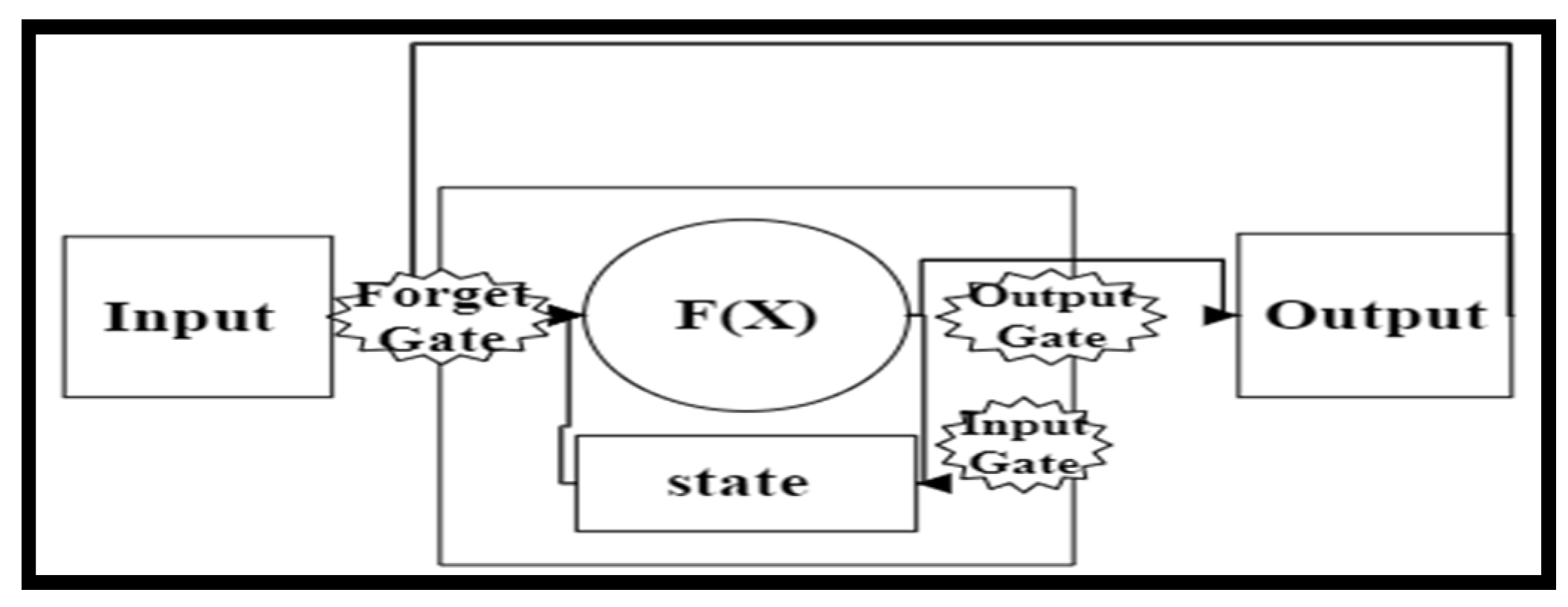
The long-short term memory, see
Figure 1, is a type of recurrent neural networks, and it is suitable for the time-series data. The name refers to the model’s ability to keep only the important information from the previous observations. Instead of neurons, the blocks in this model are called memory blocks, and each block consists of three gates and the “state”. The forget gate determines the amount of information to be used from the previous inputs. After each prediction, the input gate determines how much to save in the “state”. The output gate determines the amount of information to be used from the input and the state to predict the output. Thus, the system can recognize the trends and sequences in the data by using only the information needed for each prediction [
15].
The data taken from the factory had some negative, zero, and missing values. To deal with it, the data has been cleaned by removing all the zero and negative values and filling the missing values by the mean value for each product. LSTM can be sensitive to the scale of the data, so normalization has been carried out for the data. Then, data has been split into training and testing to evaluate the model's performance. Unlike other data sets, the data sequence has been taken into consideration while splitting the data because it is a time-series data set.
The data then were categorized into X and Y, where X is the input at t and Y is the output at t+1. The inputs are shaped into sample, time steps, and features. The LSTM model has been applied to the data and tested for its performance by root mean square error (RMSE) [
15], see
Figure 2.
4. Results and Discussion
In this work, we used the long short-term memory (LSTM) for demand forecasting of furniture sales during the Covid-19 pandemic. The model’s training data were from Jan. 2015 to Feb. 2020, while the test data were during pandemic from March 2020 to Sep. 2021.
In
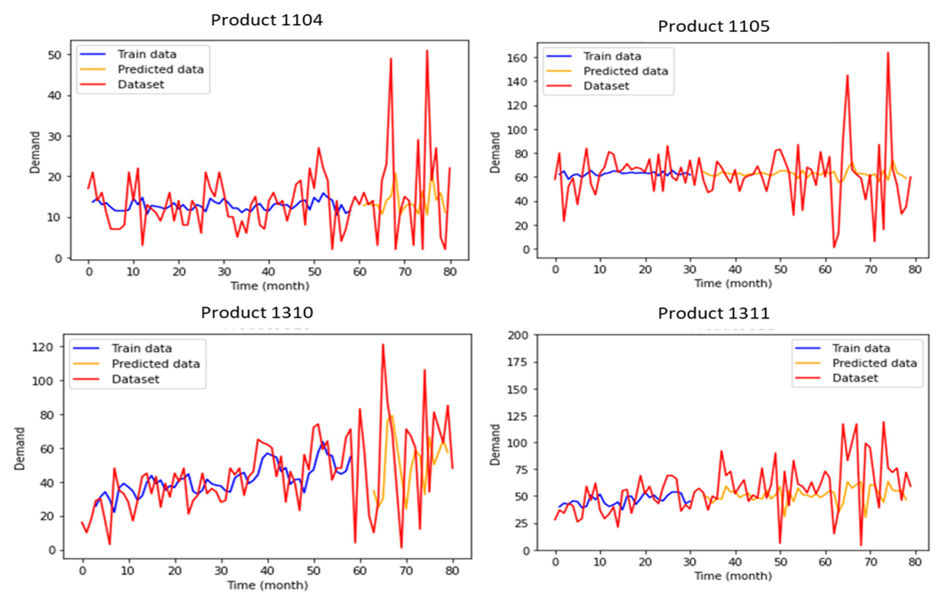
Figure 3, we presented only four out of 12 products due to limited space. From
Figure 3. we can see the plot of the predicted demand of our model. The charts present the actual dataset, predicted data, and training data. From the dataset, we can see the high variation during pandemic after month number 61 to month number 81. The heightened uncertainty and variation are due to customers’ needs and behavior changes during the pandemic.
Also, from
Figure 3, we can observe that some products data have a good fit of the LSTM model, where the model has a good fit on both the training dataset and the predicted test dataset. For example, product 1104, product 1310, and product 1311 seem to have a good fit. However, other products’ data appears to have underfitting problems, such as product 1105. The underfitting cannot predict either model, the training data, or generalize to new data. These problems occur because the model cannot capture the relationship between the output and the actual values. A further systematic study is needed to diagnose the fitting issues.
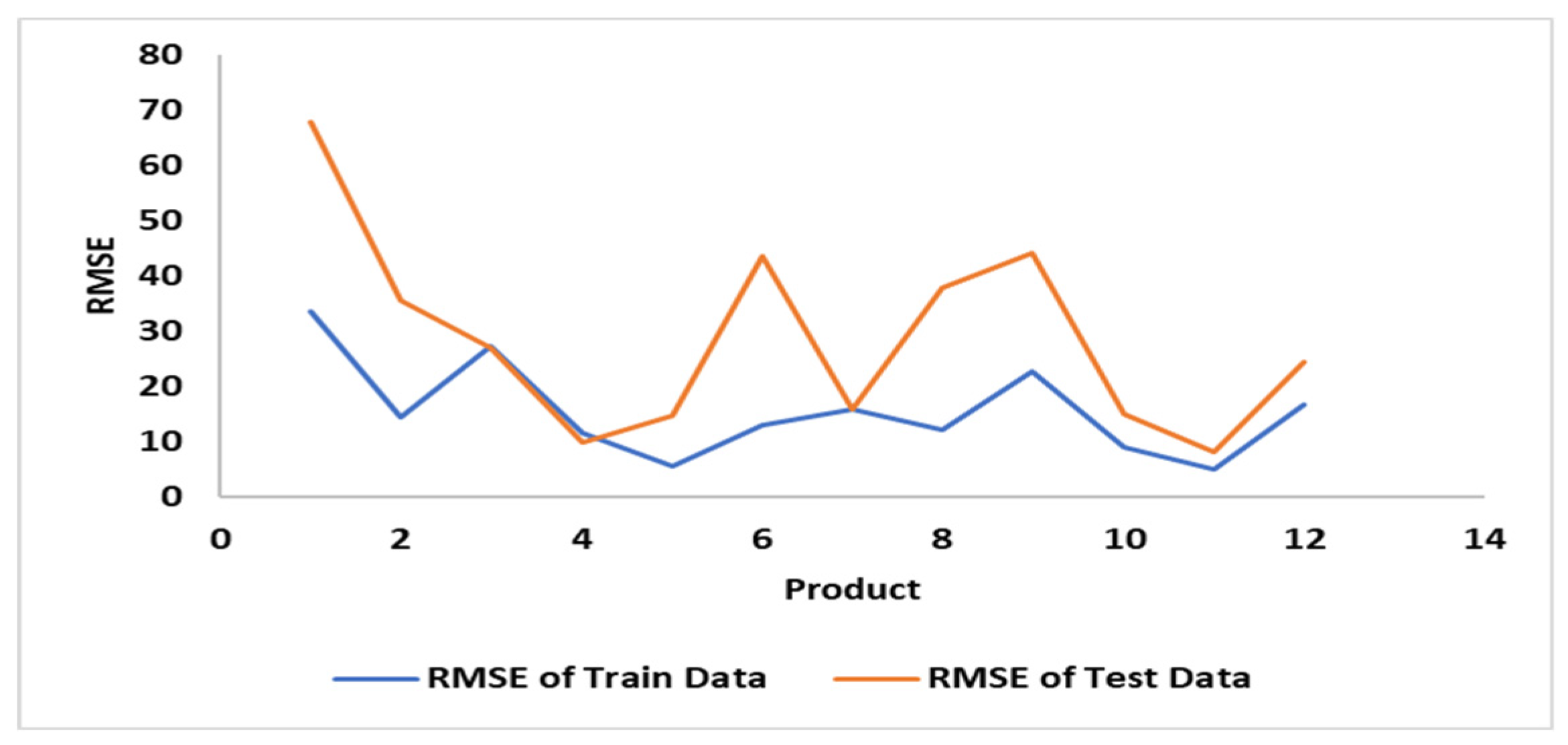
Besides the previous model evaluation by visualization of the predicted demand, we analyzed Root Mean Square Error (RMSE) in
Figure 4. RMSE tells us how robust the data is around the line of best fit.
Figure 4 shows that the RMSE of training data is lower than that of test data. This difference between RMSE values of training data and test data is due to fitting issues and the complexity of data. The complexity of data comes from seasonal behavior, and it is worsened by high variation during the Covid-19 pandemic. In addition, RMSE values have high variations within products.
The Hyperparameter optimization method was used to minimize the RMSE value for each product. Hyperparameter tuning is the method of defining the right combination of hyperparameters that helps boost model performance. Setting the proper sequence of hyperparameters is one way to obtain the high performance of models. In our model, we optimized two parameters of LSTM, which are the number of layers and neurons (1 to 20). Unfortunately, our tuning was performed manually, which was time-consuming; therefore, further work is required to make it automated and include other hyperparameter values.
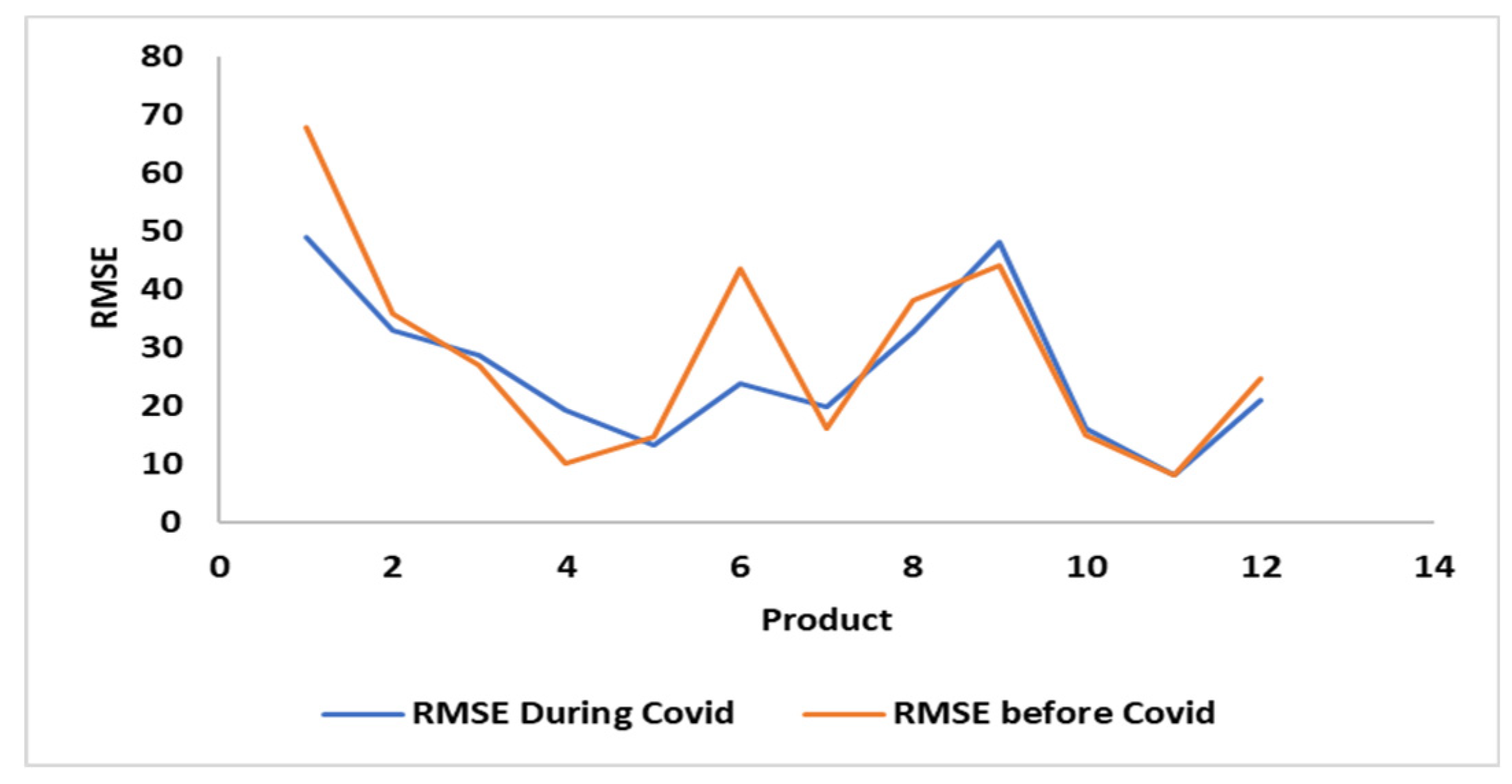
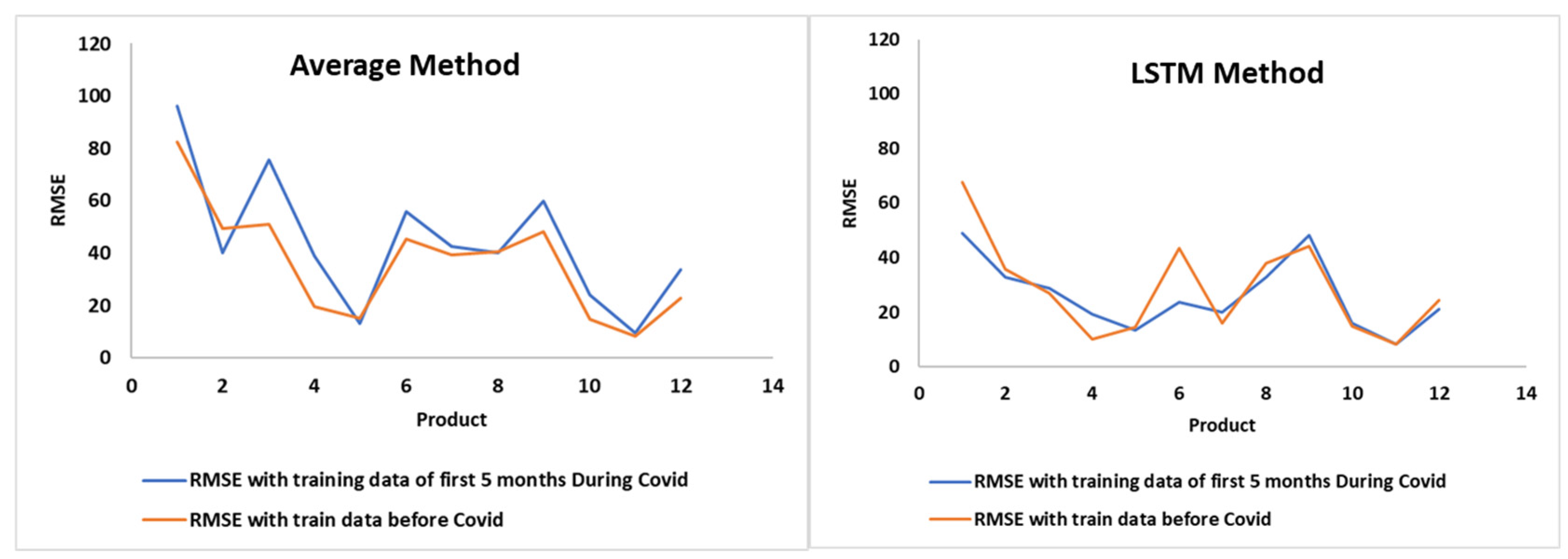
Another critical point is that we implemented fast response for the Covid-19 pandemic by using the first five months of the pandemic as training data to predict the demands of the coming months after that. The training data were from March 2020 to July 2020. The RMSE values slightly decreased for a few products, as shown in
Figure 5. Using a paired t-test with a significance level of 0.05 shows no significant difference between using the old data and the fast response to pandemic using the first five months data. However, further hyperparameters tuning and a more comprehensive training data set may show significant results.
The furniture company that provided us with data used the traditional averaging method. They averaged the demand of the previous three years and multiplied it by 1.5 in typical months, while in the season of the tax return from February to April, they multiplied the average by 2. The calculated RMSE of the averaging method shows a dramatic difference compared to our model. Using paired t-tests with a significance level of 0.05 indicated a significant difference in the mean between our model and the traditional averaging method (
Table 1 and
Figure 6). In addition, fast response by using the averaging method has worsened the prediction and increased RMSE values.
5. Conclusion and Future Work
From the previous sections, we can conclude that the Covid-19 Pandemic has caused a dramatic demand uncertainty due to customers’ needs and behavior changes. Furthermore, long short-term memory neural network has better performance than traditional demand forecasting techniques, such as averaging. In addition, neural networks can model complex data. We think that implementing a fast response to the pandemic is helpful, and it may help accommodate the variations and better demand forecasting.
Future work includes extensive hyperparameters optimization, implementing more neural network methods and comparing their performance, and investigations of fast response in more details
References
- Hoque, M.E.; Thavaneswaran, A.; Appadoo, S.S.; Thulasiram, R.K.; Banitalebi, B. A Novel Dynamic Demand Forecasting Model for Resilient Supply Chains using Machine Learning. In Proceedings of the IEEE 45th Annual Computers, 2021., Software and Applications Conference (COMPSAC).
- Meinyk, S.A.; Closs, D.J.; Griffis, S.E.; Zobel, C.W.; Macdonald, J.R. 2015. Available online: https://www.supplychain247.com/article/understanding supply chain resilience.
- Nagaraja, C.H.; Thavaneswaran, A.; Appadoo, S.S. Measuring the bullwhip effect for supply chains with seasonal demand components”. European Journal of Operational Research 2015, 242, 445–454. [Google Scholar] [CrossRef]
- Baltas, G. Modelling category demand in retail chains. The Journal of the Operational Research Society 2005, 56, 1258–1264. [Google Scholar]
- Goic, M.; Bozanic-Leal, M.S.; Badal, M.; Basso, L.J. “COVID-19: Short-term forecast of ICU beds in times of crisis”. PLoS ONE 2021, 16, e0245272. [Google Scholar] [CrossRef]
- Bates, J.M.; Granger, C.W.J. “The Combination of Forecasts”. Journal of the Operational Research Society 1969, 20, 451–468. [Google Scholar] [CrossRef]
- Sharma, S.K.; Sharma, V. “Comparative Analysis of Machine Learning Techniques in Sale Forecasting”. International Journal of Computer Applications 2012, 53, 445–454. [Google Scholar]
- Carbonneau, R.; Laframboise, K.; Vahidov, R. “Application of machine learning techniques for supply chain demand forecasting”. European Journal of Operational Research 2008, 184, 1140–1154. [Google Scholar] [CrossRef]
- Chartoniuk, W.; Box, E.D.; Lee, W.-J.; Chen, M.-S.; Kotas, P.; Olinda, P.V. “Neural-Network-Based Demand Forecasting in a Deregulated Environment”. IEEE Transactions on Industry Applications 2000, 36, 893–898. [Google Scholar] [CrossRef]
- Sen, R.; Yu, H.-F.; Dhillon, I. “Think Globally, Act Locally: A Deep Neural Network Approach to High- Dimensional Time Series Forecasting”. Amazon and UT Austin. 2019.
- Tighe, D. “Coronavirus: Monthly retail; sales development by sector, US 2021. Statista”. Retrieved , 2021. 19 September 1104. Available online: https://www.statista.com/statistics/1104316/coronavirus-month-over-month-retail-sales-development-by-sector-us/.
- Vidojevic, B. “Online Furniture Sales During and Post-Covid-19”. Retrieved , 2021. 19 September. Available online: https://www.statista.com/statistics/1104316/coronavirus-month-over-month-retail-sales-development-by-sector-us/.
- Vogels, T.P.; Rajan, K.; Abbott, L.F. “Neural network dynamics”. Annu. Rev. Neurosci.. 2005, 28, 357–76. [Google Scholar] [CrossRef]
- 14. W. Zaremba ,I. Sutskever ,O. Vinyals . “Recurrent neural network regularization”. arXiv, arXiv:1409.2329.
- Hochreiter, S.; Schmidhuber, J. “Long short-term memory”. Neural computation. 1997, 9, 1735–80. [Google Scholar] [CrossRef]
|
Disclaimer/Publisher’s Note: The statements, opinions and data contained in all publications are solely those of the individual author(s) and contributor(s) and not of MDPI and/or the editor(s). MDPI and/or the editor(s) disclaim responsibility for any injury to people or property resulting from any ideas, methods, instructions or products referred to in the content. |
© 2023 by the authors. Licensee MDPI, Basel, Switzerland. This article is an open access article distributed under the terms and conditions of the Creative Commons Attribution (CC BY) license (http://creativecommons.org/licenses/by/4.0/).
