A Polar Moving-Base Alignment Based on Backtracking Scheme

Preprint

Article

A Polar Moving-Base Alignment Based on Backtracking Scheme

Altmetrics

Downloads

120

Views

Comments

A peer-reviewed article of this preprint also exists.

This version is not peer-reviewed

Submitted:

10 April 2023

Posted:

10 April 2023

You are already at the latest version

Alerts

Abstract

In the polar region, the gravity vector and Earth's rotation vector tend to be in the same direction, leading to slower convergence speed and longer alignment time of the moving base alignment. When the alignment time is short, the alignment cannot converge, resulting in low azimuth accuracy. To address this issue, we propose a polar moving base alignment method based on backtracking scheme. Notably, this work first derives a polar coarse alignment method with the inertial frame based on the transverse Earth model. On this basis, we design a polar coarse alignment method based on backtracking scheme and optimize the data storage scheme. Then, an inverse navigation algorithm based on the transverse inertial navigation mechanical arrangement scheme was derived, and a polar fine alignment method based on backtracking scheme was designed. Semi-physical simulation experiments showed that the alignment algorithm based on backtracking scheme can converge in a short time with high alignment accuracy.

Keywords:

Subject: Engineering - Marine Engineering

1. Introduction

In recent years, global warming has accelerated the melting of polar ice caps, leading to an increase in the value of strategic, economic, scientific, environmental, navigational, and resource in the polar region [1]. To achieve smooth and safe navigation or operations in the polar region, various types of marine carriers must rely on high-precision navigation systems [2]. The high-precision strapdown inertial navigation system (SINS) has become the core navigation technology to meet the application of polar regions with its autonomy and resistance to external environmental interference [3]. As one of the key technologies of SINS, moving base alignment is also a research hotspot in the field of polar navigation.

Auxiliary navigation information is necessary to achieve the moving base alignment. However, the arctic geophysical field may impair the electrical or optical-based auxiliary navigation systems [4,5], resulting in performance degradation or even failure occurs, which in turn lead to alignment failure. For example, affected by intense magnetic storms, the accuracy of Global Navigation Satellite System (GNSS) decreases, and sometimes even fails. Moreover, common meteorological conditions in the polar region, such as fog, low clouds, snow, and polar night, limit the visibility, which affects the observation of starlight by astronomical navigation sensors, rendering astronomical navigation unusable. In contrast, the Doppler Velocity Log (DVL) is preferred to assist in moving base alignment since it is not affected by the unique geography of the polar region [6].

The initial alignment process is divided into two stages: coarse alignment and fine alignment [7]. The main task of the coarse alignment is to obtain a rough attitude matrix of the carrier in a short time and provide it to the fine alignment [8]. The fine alignment aims to obtain a high-precision attitude matrix of the carrier, which takes a long time to complete [9].

The coarse alignment of the moving base is usually achieved through the use of inertial alignment methods [10,11,12,13]. In the polar region, the convergence of meridians with increasing latitude leads to the amplification of longitude errors, which increases the alignment error of traditional inertial alignment algorithms that involve longitude terms in the solution process. To address this issue, Liu proposed a polar inertial-frame alignment algorithm with pseudo-SINS modeling, which eliminated the impact of longitude error amplification on polar alignment [13]. However, the use of a spherical Earth model in the pseudo-SINS modeling leads to the principle error in this alignment algorithm, while the transverse Earth ellipsoid model is an ellipsoidal model, and there is no amplification of errors in the transverse latitude and longitude directions in the polar region [14]. Therefore, this paper designs a

V^{b}

aided inertial alignment algorithm under the transverse Earth model to eliminate the principle error and the amplification of longitude errors.

During the fine alignment of the moving base, an integrated alignment method is usually used [15,16,17,18,19]. In the polar region, as the latitude increases, the gravity vector and Earth's rotation vector tend to be in the same direction, the gyrocompass effect weakens, and the azimuth accuracy of the coarse alignment of the inertial system decreases. This results in difficulties in achieving the integrated alignment aided by DVL under small misalignment. To address this issue, Wang proposed a DVL-aided integrated alignment algorithm for large misalignment angle in the polar region [18]. However, linearization was performed when deriving the differential equation of the velocity error, resulting in large azimuth errors of the alignment. Liu re-derived the DVL-aided integrated alignment algorithm under large azimuth misalignment, which improved the azimuth accuracy [19].

Currently, research on polar alignment algorithms has focused on improving alignment accuracy, but not on alignment speed. In order to improve the alignment speed of SINS, [20,21,22] have proposed integrated fine alignment methods based on a backtracking scheme, which effectively shortens the alignment time. In the polar region, the gyrocompass effect weakens, and the convergence time of the inertial-frame coarse alignment is increased, resulting in the coarse alignment time exceeding the backtracking fine alignment time. Therefore, when designing a polar region backtracking alignment algorithm, not only a backtracking fine alignment algorithm needs to be designed, but also a backtracking coarse alignment algorithm needs to be designed to shorten the coarse alignment time. Reference [23] proposed a backtracking coarse alignment algorithm that effectively shortens the coarse alignment time. However, their research was implemented based on the North mechanics arrangement and cannot be directly applied to the polar region. In addition, during the backtracking coarse alignment process, the parameters in the backward coarse alignment update process have already been calculated in the forward coarse alignment update process. Recalculating the parameters using the gyroscope and accelerometer data in the backward coarse alignment update process will lead to wasted computational resources. Furthermore, the integrated fine alignment algorithm under large azimuth misalignment in the polar region can quickly reduce the azimuth error to small misalignment. Therefore, when designing the polar backtracking fine alignment algorithm, the large azimuth misalignment integrated fine alignment algorithm only needs to be run once, and subsequent backtracking fine alignment process can be realized using the small misalignment integrated fine alignment algorithm.

Based on the above analysis, this paper proposes a moving base backtracking alignment method in the polar region. The main contribution of this paper is the derivation of an auxiliary inertial alignment algorithm under transverse Earth model, which improves the coarse alignment accuracy in the polar region. On this basis, a polar coarse alignment and fine alignment method based on backtracking scheme were designed, which shortened the alignment time for both coarse and fine alignment. The structure of this paper is as follows: Section 2 introduces all frames involved in the polar backtracking alignment algorithm, derives the polar coarse alignment method with the inertial frame based on the transverse Earth model, and introduces the polar fine alignment algorithm. Section 3 proposes the polar coarse and fine alignment methods based on backtracking scheme. Section 4 analyzes the experimental results. Finally, Section 5 gives the conclusion.

2. The Polar Coarse and Fine Alignment Methods

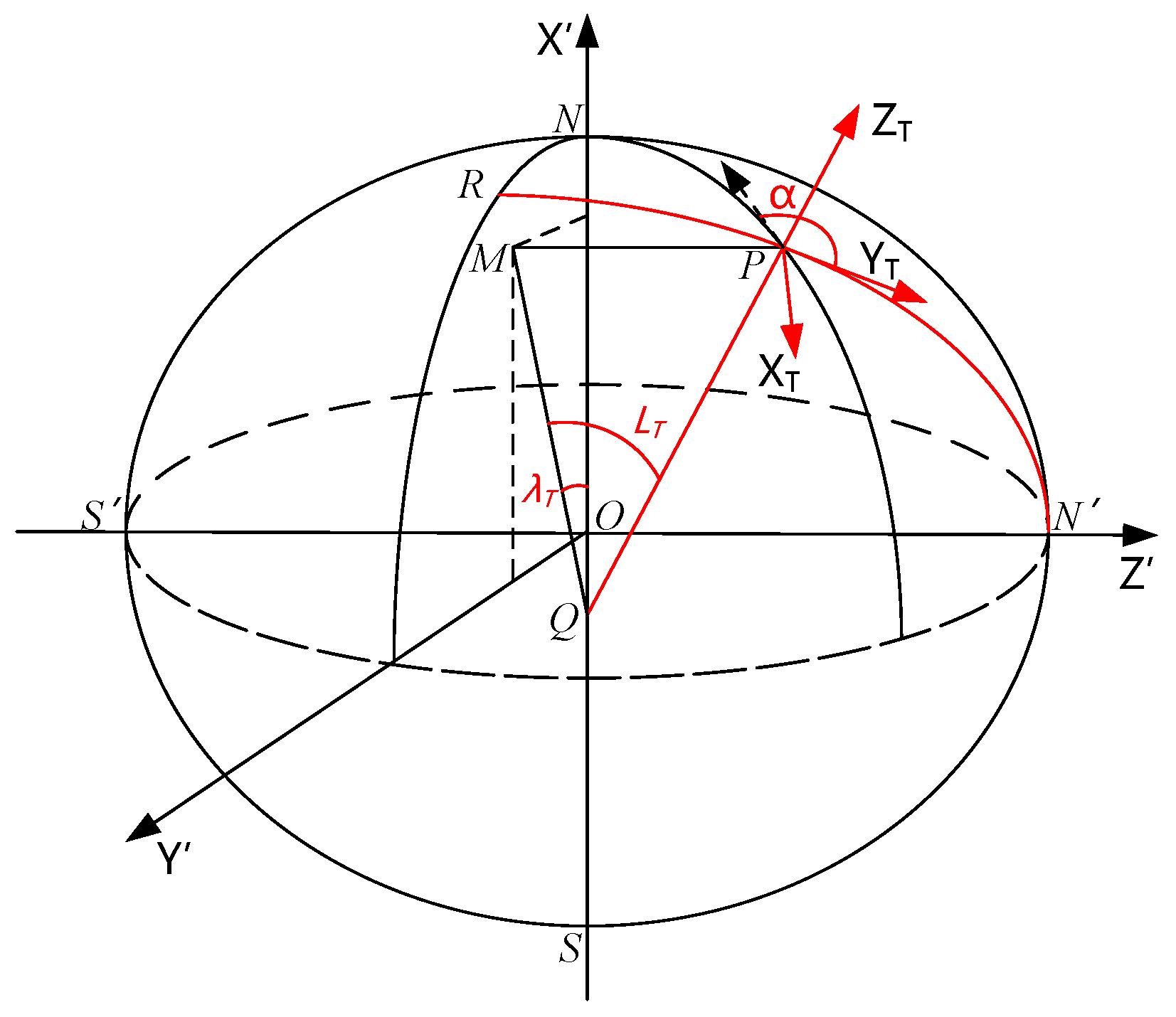
In this section, the frames used in the polar coarse and fine alignments are firstly introduced. Then, the polar coarse alignment method with the inertial frame based on the transverse Earth model is derived to eliminate the effect of the polar alignment algorithm caused by longitude error amplification. Finally, the integrated fine alignment algorithm under large azimuth misalignment and the integrated fine alignment algorithm under small misalignment used in the backtracking fine alignment process are respectively introduced in the polar region.

2.1 Transverse Earth Model and the Definition of Transverse Frame

The definition of the transverse Earth model and the inertial navigation arrangement in this paper are consistent with reference [14], as shown in Figure 1. In the transverse Earth model, the transverse North Pole is the intersection point between the 90°E meridian and the equator, the transverse equator is the meridian circle composed of the 0° and 180° meridians, and the transverse prime meridian is the meridian circle composed of the 90°E and 90°W meridians. The transverse latitude

L_{T}

is the angle between the normal

P Q

of point

P

on the ellipsoid and the transverse equatorial plane, and the transverse longitude

λ_{T}

is the angle between the projection

M Q

P Q

on the transverse equatorial plane and

X'

axis.

Following reference [14], the transformation matrix between the Earth frame and the transverse Earth frame is as follows:

C_{e}^{e_{T}} = [\begin{matrix} 0 & 0 & 1 \\ 1 & 0 & 0 \\ 0 & 1 & 0 \end{matrix}]

(1)

To facilitate subsequent problem description and formula derivation, all frames involved in the algorithm are defined as right-handed Cartesian frames, which are defined as follows:

The Earth-Centered inertial frame $i$ : the origin $o_{i}$ is at the center of the Earth, the $o_{i} x_{i}$ axis points towards the vernal equinox, the $o_{i} z_{i}$ axis points towards the north pole;
Earth-Fixed frame $e$ : the origin $o_{e}$ is at the center of the Earth, the $o_{e} x_{e}$ axis points to the prime meridian, the $o_{e} z_{e}$ axis points to the north pole;
The transverse Earth frame $e_{T}$ : The origin $o_{e T}$ is at the center of the Earth, the $o_{e T} x_{e T}$ axis points to the transverse prime meridian, the $o_{e T} z_{e T}$ axis points to the transverse north pole;
The transverse geographic frame $T$ : The origin $o_{T}$ is the center of mass of the carrier. The $o_{T} y_{T}$ axis points to the north in the transverse direction, the $o_{T} z_{T}$ axis is perpendicular to the local transverse plane and points to the sky;
The body frame $b$ : The origin $o_{b}$ is at the center of mass of the body. The $o_{b} x_{b}$ axis points to the right of the body, the $o_{b} y_{b}$ axis points forward along the longitudinal axis, and the $o_{b} z_{b}$ axis points upward along the body axis;
The initial transverse inertial frame $i_{T 0}$ : The origin $o_{i T 0}$ is at the center of the Earth, the $o_{i T 0} z_{i T 0}$ axis points to the transverse North Pole, the $o_{i T 0} x_{i T 0}$ axis is parallel to the $Q M$ in the transverse equatorial plane;
The initial transverse Earth frame $e_{T 0}$ : The frame $e_{T}$ at the initial moment;
The initial transverse geographic frame $T_{0}$ : The frame $T$ at the initial moment;
The initial body frame $i_{b 0}$ : At the initial moment, the frame $i_{b 0}$ coincides with the frame $b$ , and after the alignment begins, the frame $i_{b 0}$ remains fixed and does not move with the body.

Among them, the frame

i

i_{T 0}

and

i_{b 0}

remain fixed in the inertial space and do not change with time. The frame

e

e_{T}

e_{T 0}

and

T_{0}

maintain the same orientation as the Earth's motion. The frame

b

and

T

are fixed to the body.

2.2. The inertial-frame coarse alignment algorithm aided by the $V^{b}$ based on the transverse Earth model.

In the polar moving base alignment algorithm, all time-varying variables are represented in

\cdot (t)

. The attitude matrix

C_{b}^{T} (t)

at time

t

is decomposed into the product of three matrices as follows:

C_{b}^{T} (t) = C_{i_{T 0}}^{T} (t) C_{i_{b 0}}^{i_{T 0}} C_{b}^{i_{b 0}} (t)

(2)

where

C_{i_{T 0}}^{T} (t)

is the transformation matrix from the frame

i_{T 0}

to the frame

T

under the horizontal Earth model.

C_{b}^{i_{b 0}} (t)

is the attitude matrix of the frame

b

relative to the frame

i_{b 0}

, both of which can be obtained through navigation information.

C_{i_{b 0}}^{i_{T 0}}

is the attitude matrix of the frame

i_{b 0}

relative to the frame

i_{T 0}

under the transverse Earth model, which is a constant matrix.

Based on the analysis above,

C_{i_{T 0}}^{T} (t)

can be obtained as follows:

C_{i_{T 0}}^{T} (t) = C_{e_{T}}^{T} (t) {(C_{e_{T}}^{e_{T 0}})}^{T} C_{i_{T 0}}^{e_{T 0}} (t)

(3)

where

C_{e_{T}}^{T} (t)

and

C_{e_{T}}^{e_{T 0}}

can be obtained from the transverse longitude and latitude of the body's location, and

C_{i_{T 0}}^{e_{T 0}} (t)

can be obtained in real time using the Earth's rotation rate

ω_{i e}^{e}

and the transverse longitude

λ_{T 0}

of the body's location at the initial moment.

C_{b}^{i_{b 0}} (t)

is the attitude matrix of the frame

b

relative to the frame

i_{b 0}

C_{e_{T}}^{T} (t) = [\begin{matrix} - \sin λ_{T} (t) & \cos λ_{T} (t) & 0 \\ - \sin L_{T} (t) \cos λ_{T} (t) & - \sin L_{T} (t) \sin λ_{T} (t) & \cos L_{T} (t) \\ \cos L_{T} (t) \cos λ_{T} (t) & \cos L_{T} (t) \sin λ_{T} (t) & \sin L_{T} (t) \end{matrix}]

(4)

where

λ_{T} (t)

and

L_{T} (t)

represent the transverse longitude and latitude of the body location at

t

C_{e_{T}}^{e_{T 0}} = [\begin{matrix} \cos λ_{T 0} & \sin λ_{T 0} & 0 \\ - \sin λ_{T 0} & \cos λ_{T 0} & 0 \\ 0 & 0 & 1 \end{matrix}]

(5)

C_{e_{T 0}}^{i_{T 0}} (t) = C_{e_{T 0}}^{i_{T 0}} (t - 1) C_{e_{T 0} (t)}^{e_{T 0} (t - 1)}

(6)

C_{e_{T 0} (t)}^{e_{T 0} (t - 1)} = I_{3 \times 3} + \frac{\sin |ϕ_{i e_{T 0}}^{e_{T 0}}|}{|ϕ_{i e_{T 0}}^{e_{T 0}}|} [ϕ_{i e_{T 0}}^{e_{T 0}} \times] + \frac{1 - \cos |ϕ_{i e_{T 0}}^{e_{T 0}}|}{{|ϕ_{i e_{T 0}}^{e_{T 0}}|}^{2}} {[ϕ_{i e_{T 0}}^{e_{T 0}} \times]}^{2}

(7)

where the initial value of matrix

C_{e_{T 0}}^{i_{T 0}} (t)

is the identity matrix

C_{e_{T 0}}^{i_{T 0}} (0) = I_{3 \times 3}

, i.e.,

C_{e_{T 0} (t)}^{e_{T 0} (t - 1)}

is the change in rotation of the frame

e_{T 0}

relative to the frame

i

from time

t - 1

to time

t

ϕ_{i e_{T 0}}^{e_{T 0}}

is the equivalent rotation vector of the frame

e_{T 0}

relative to the reference frame

i

from time

t - 1

to time

t

, which can be obtained from the angular velocity

ω_{i e_{T 0}}^{e_{T 0}}

between frame

e_{T 0}

and frame

i

ω_{i e_{T 0}}^{e_{T 0}}

is always constant, it can be derived that:

ϕ_{i e_{T 0}}^{e_{T 0}} = T ω_{i e_{T 0}}^{e_{T 0}}

(8)

\begin{matrix} ω_{i e_{T 0}}^{e_{T 0}} & = C_{e_{T}}^{e_{T 0}} C_{e}^{e_{T}} (ω_{i e}^{e} + ω_{e e_{T 0}}^{e}) = C_{e_{T}}^{e_{T 0}} C_{e}^{e_{T}} ω_{i e}^{e} \\ = {[ω_{i e} \cos λ_{T 0} - ω_{i e} \sin λ_{T 0} 0]}^{T} \end{matrix}

(9)

where

T

is the duration of period

[t - 1, t]

ω_{i e}

is the angular rate of Earth rotation.

C_{i_{T 0}}^{T} (t)

can be obtained by solving from (4)–(9).

Then,

C_{b}^{i_{b 0}} (t)

can be calculated by the following equation

C_{b}^{i_{b 0}} (t) = C_{b}^{i_{b 0}} (t - 1) C_{b (t)}^{b (t - 1)}

(10)

where the initial value of matrix

C_{b}^{i_{b 0}} (t)

is the identity matrix

C_{b}^{i_{b 0}} (0) = I_{3 \times 3}

, i.e.,

C_{b (t)}^{b (t - 1)}

can be calculated in real-time through the equivalent rotation vector

ϕ_{i b}^{b} (t)

C_{b (t)}^{b (t - 1)} = I_{3 \times 3} + \frac{\sin |ϕ_{i b}^{b} (t)|}{|ϕ_{i b}^{b} (t)|} [ϕ_{i b}^{b} (t) \times] + \frac{1 - \cos |ϕ_{i b}^{b} (t)|}{{|ϕ_{i b}^{b} (t)|}^{2}} {[ϕ_{i b}^{b} (t) \times]}^{2}

(11)

ϕ_{i b}^{b} (t)

can be solved using the "single-sample + previous cycle" algorithm with the inertial navigation sampled angle increment

Δ θ

ϕ_{i b}^{b} (t) = Δ θ (t) + \frac{1}{12} Δ θ (t - 1) \times Δ θ (t)

(12)

According to the matrix decomposition in equation (2), the calculation of the transformation matrix

C_{b}^{T} (t)

can be coverted into the calculation of a fixed matrix

C_{i_{b 0}}^{i_{T 0}}

. This transforms a traditional time-varying attitude error estimation problem into a time-invariant attitude error estimation problem.

According to the SINS attitude and velocity update equation, we can obtain:

{\dot{C}}_{b}^{T} (t) = C_{b}^{T} (t) (ω_{T b}^{b} (t) \times)

(13)

{\dot{V}}^{T} (t) = C_{b}^{T} (t) f^{b} (t) - (2 ω_{i e_{T}}^{T} (t) + ω_{e_{T} T}^{T} (t)) \times V^{T} (t) + G^{T}

(14)

V^{T} (t) = C_{b}^{T} (t) V^{b} (t)

(15)

where

ω_{T b}^{b} (t)

is the projection of the angular velocity between the frame

b

and frame

T

onto the frame

b

V^{T} (t)

and

V^{b} (t)

are the vehicle velocities in the frame

T

and frame

b

, respectively,

V^{b} (t)

is measured by DVL,

f^{b} (t)

is the output of the ideal accelerometer,

ω_{e_{T} T}^{T} (t)

is the projection of the frame

T

relative to the frame

e_{T}

onto the frame

T

, and

ω_{i e_{T}}^{T} (t)

and

G^{T}

are the projections of the Earth's rotation rate and gravitational acceleration onto the frame

T

Taking the derivative of both sides of (15) and substituting (13), we obtain:

{\dot{V}}^{T} (t) = {\dot{C}}_{b}^{T} (t) V^{b} (t) + C_{b}^{T} (t) {\dot{V}}^{b} (t) = C_{b}^{T} (t) [{\dot{V}}^{b} (t) + ω_{T b}^{b} (t) \times V^{b} (t)]

(16)

By substituting (16) into (14) and simplifying, we obtain:

C_{b}^{T} (t) [{\dot{V}}^{b} (t) + (ω_{i e_{T}}^{b} (t) + ω_{i b}^{b} (t)) \times V^{b} (t) - f^{b} (t)] = G^{T}

(17)

By substituting (2) into (17) and simplifying, we obtain:

C_{i_{b 0}}^{i_{T 0}} C_{b}^{i_{b 0}} (t) [{\dot{V}}^{b} (t) + (ω_{i e_{T}}^{b} (t) + ω_{i b}^{b} (t)) \times V^{b} (t) - f^{b} (t)] = C_{T}^{i_{T 0}} (t) G^{T}

(18)

In order to reduce the influence of DVL velocity measurement errors and accelerometer measurement errors, integrating both sides of Equation (18) and simplifying, we can obtain the velocity vector observation aided by DVL velocity

V^{b} (t)

C_{i_{b 0}}^{i_{T 0}} α^{b} (t) = β^{b} (t)

(19)

where,

α^{b} (t) = C_{b}^{i_{b 0}} (t) V^{b} (t) - V^{b} (0) + \int_{0}^{t} C_{b}^{i_{b 0}} (t) [ω_{i e_{T}}^{b} (t) \times V^{b} (t) - f^{b} (t)] d t

(20)

β^{b} (t) = \int_{0}^{t} C_{T}^{i_{T 0}} (t) G^{T} d t

(21)

According to Equation (19), the solution for

C_{i_{b 0}}^{i_{T 0}}

is coverted into a Wahba problem when

α^{b} (t)

and

β^{b} (t)

are known [24]. For the Wahba problem, the singular value decomposition (SVD) algorithm and quaternion-based methods such as q-method, are essentially equivalent in results, but the SVD algorithm is more concise and intuitive [25]. Therefore, the SVD method is used to solved. The specific solution method is as follows:

A = \sum_{t = 1}^{t_{1}} β^{b} (t) {[α^{b} (t)]}^{T}

(22)

where the variable

t_{1}

represents the end time of the alignment process.

Matrix A can be decomposed using SVD as follows:

A = U [\begin{matrix} σ_{1} & 0 & 0 \\ 0 & σ_{2} & 0 \\ 0 & 0 & σ_{3} \end{matrix}] V^{T}

(23)

where

σ_{i} (i = 1, 2, 3)

is the singular value of matrix

A

The attitude transformation matrix can be obtained from this equation.

C_{i_{b 0}}^{i_{T 0}} = U V^{T}

(24)

Due to the unknown

C_{b}^{T} (t)

before coarse alignment and the unavailability of real-time position information other than the velocity information provided by DVL, there are two approximations made in the computation of the constant matrix

C_{i_{b 0}}^{i_{T 0}}

during the moving base coarse alignment process. Firstly, in Equation (4), the initial position information is used as a substitute when calculating

C_{e_{T}}^{T} (t)

. Secondly, in Equation (20), the variable

ω_{i e_{T}}^{b} (t) \times V^{b} (t)

is ignored because

ω_{i e_{T}}^{b} (t)

is unknown. Therefore, the actual computation of Equations (4) and (20) are as follows:

C_{e_{T}}^{T} (t) = [\begin{matrix} - \sin λ_{T 0} & \cos λ_{T 0} & 0 \\ - \sin L_{T 0} \cos λ_{T 0} & - \sin L_{T 0} \sin λ_{T 0} & \cos L_{T 0} \\ \cos L_{T 0} \cos λ_{T 0} & \cos L_{T 0} \sin λ_{T 0} & \sin L_{T 0} \end{matrix}]

(25)

α^{b} (t) = C_{b}^{i_{b 0}} (t) V^{b} (t) - V^{b} (0) - \int_{0}^{t} C_{b}^{i_{b 0}} (t) f^{b} (t) d t

(26)

where the variables

λ_{T 0}

and

L_{T 0}

represent the initial transverse longitudinal and latitudinal positions of the body, respectively.

However, it should be noted that the approximation in calculating

C_{i_{b 0}}^{i_{T 0}}

results in relatively large errors. However, in the process of solving

C_{b}^{T} (t)

in Equation (2), both

C_{i_{b 0}}^{i_{T 0}}

and

C_{e_{T}}^{T} (t)

contain the error caused by the first approximation, and the errors partially offset each other. As a result, the accuracy of

C_{b}^{T} (t)

is higher than that of

C_{i_{b 0}}^{i_{T 0}}

when coarse alignment is completed.

In summary, the attitude matrix

C_{b}^{T} (t)

can be obtained by using equations (2)-(12) and (19)-(26) to achieve coarse alignment of the moving base. In the backward process, the initial attitude

C_{b}^{T} (0)

can be calculated by substituting the obtained

C_{i_{b 0}}^{i_{T 0}}

from the coarse alignment into Equation (2).

2.3. The polar Fine Alignment Method assisted by DVL under Large Azimuth Misalignment

The integrated alignment algorithm assisted by DVL under large azimuth misalignment angle used in this paper is consistent with the approach in reference [19]. Based on the nonlinear error equations of transverse inertial navigation, a state model is established. The velocity information from DVL is used to establish a measurement model. The adaptive unscented Kalman filter (UKF) algorithm is employed to achieve alignment. The state and measurement models are shown below.

The model can ignore altitude velocity error

δ v_{u}^{T}

and height error

δ h

. The platform misalignment

ϕ^{T}

, transverse horizontal velocity error

[\begin{matrix} δ v_{e}^{T} & δ v_{n}^{T} \end{matrix}]

, transverse longitude and latitude error

[\begin{matrix} δ L_{T} & δ λ_{T} \end{matrix}]

, constant gyro drift

ε^{b}

, and accelerometer bias

\nabla^{b}

are selected as states.

X = {[\begin{matrix} ϕ_{x}^{T} & ϕ_{y}^{T} & ϕ_{z}^{T} & δ v_{e}^{T} & δ v_{n}^{T} & δ L_{T} & δ λ_{T} & ε_{x} & ε_{y} & ε_{z} & \nabla_{x} & \nabla_{y} & \nabla_{z} \end{matrix}]}^{T}

(27)

The state equation can be obtained as follows:

\{\begin{matrix} {\dot{ϕ}}^{T} & = C_{ω}^{- 1} [(I - C_{T}^{T'}) {\hat{ω}}_{i T}^{T} + C_{T}^{T'} δ ω_{i T}^{T} - C_{b}^{T'} ε^{b}] \\ δ {\dot{V}}^{T} & = (I - C_{T'}^{T}) C_{b}^{T'} {\hat{f}}^{b} + C_{T'}^{T} C_{b}^{T'} \nabla^{b} - (2 δ ω_{i e_{T}}^{T} + δ ω_{e_{T} T}^{T}) \times {\hat{V}}^{T} \\ - (2 {\hat{ω}}_{i e_{T}}^{T} + {\hat{ω}}_{e_{T} T}^{T}) \times δ V^{T} \\ δ {\dot{L}}_{T} & = - \frac{2 {\hat{v}}_{b}}{\hat{τ} \sin 2 {\hat{λ}}_{T}} δ λ_{T} + \frac{{\hat{v}}_{b}}{\hat{τ} \tan {\hat{L}}_{T}} δ L_{T} - \frac{1}{\hat{τ}} δ v_{e}^{T} + \frac{1}{{\hat{R}}_{y}} δ v_{n}^{T} \\ δ {\dot{λ}}_{T} & = \frac{1}{{\hat{R}}_{x} \cos {\hat{L}}_{T}} δ v_{e}^{T} - \frac{1}{\hat{τ} \cos {\hat{L}}_{T}} δ v_{n}^{T} + \frac{2 {\hat{v}}_{a}}{\hat{τ} \cos {\hat{L}}_{T} \sin 2 {\hat{λ}}_{T}} δ λ_{T} \\ + (\frac{{\hat{v}}_{e}^{T}}{{\hat{R}}_{x} \cos^{2} {\hat{L}}_{T}} - \frac{{\hat{v}}_{n}^{T} \tan {\hat{L}}_{T} + {\hat{v}}_{a}}{\hat{τ} \cos {\hat{L}}_{T} \tan {\hat{L}}_{T}}) δ L_{T} \\ {\dot{ε}}^{b} & = 0 \\ {\dot{\nabla}}^{b} & = 0 \end{matrix}

(28)

where,

C_{ω}^{- 1} = [\begin{matrix} 1 & 0 & ϕ_{y}^{T} \\ 0 & 1 & - ϕ_{x}^{T} \\ - ϕ_{y}^{T} & 0 & 1 \end{matrix}]

(29)

\{\begin{cases} \frac{1}{τ} = (\frac{1}{R_{M}} - \frac{1}{R_{N}}) \sin α \cos α \\ \frac{1}{R_{x}} = \frac{\sin^{2} α}{R_{M}} + \frac{\cos^{2} α}{R_{N}} \\ \frac{1}{R_{y}} = \frac{\cos^{2} α}{R_{M}} + \frac{\sin^{2} α}{R_{N}} \end{cases}

(30)

\{\begin{cases} {\hat{v}}_{a} = {\hat{v}}_{e}^{T} \sin 2 \hat{α} - {\hat{v}}_{n}^{T} \cos 2 \hat{α} \\ {\hat{v}}_{b} = {\hat{v}}_{e}^{T} \cos 2 \hat{α} + {\hat{v}}_{n}^{T} \sin 2 \hat{α} \end{cases}

(31)

where

C_{T}^{T'}

represents the attitude matrix between the computed navigation frame

T'

and frame

T

，

{\hat{ω}}_{i T}^{T}

represents the calculated value of commanded angular velocity,

δ ω_{i T}^{T}

represents the navigation frame calculation error,

C_{b}^{T'}

represents the calculated value of attitude matrix,

{\hat{f}}^{b}

represents the output of actual acceleration,

{\hat{ω}}_{i e_{T}}^{T}

represents the calculated value of the projection of Earth's rotation angular velocity in frame

T

{\hat{ω}}_{e_{T} T}^{T}

represents the calculated value of the projection of frame

T

relative to frame

e_{T}

in frame

T

δ ω_{i e_{T}}^{T}

represents the calculation error of Earth's rotation angular velocity,

δ ω_{e_{T} T}^{T}

represents the calculation error of the navigation system rotation angular velocity,

{\hat{V}}^{T}

represents the calculated value of the carrier velocity in frame

T

δ V^{T}

represents the error of the carrier velocity in frame

T

{\hat{L}}_{T}

and

{\hat{λ}}_{T}

represent the calculated values of the transverse latitude and longitude, respectively,

δ L_{T}

and

δ λ_{T}

represent the errors of the transverse latitude and longitude, respectively,

{\hat{v}}_{e}^{T}

and

{\hat{v}}_{n}^{T}

represent the calculated values of the transverse eastward and northward velocity, respectively,

ϕ_{x}^{T}

and

ϕ_{y}^{T}

represent the attitude angles of rotation around the x-axis and y-axis, respectively,

R_{M}

and

R_{N}

represent the curvature radii of the Earth's meridian and transverse circles, respectively, and

α

represents the angle between frame

T

and the local geographic frame

g

The measurement equation for the difference between the velocity provided by SINS and DVL in frame

T

is given by:

\begin{matrix} Z_{D V L} = {\hat{V}}_{S I N S}^{T} - {\hat{V}}_{D V L}^{T} = {\hat{V}}_{S I N S}^{T} - C_{T}^{T'} ({\hat{V}}_{S I N S}^{T} - δ V_{S I N S}^{T}) - δ V_{D V L}^{T'} \\ = (I - C_{T}^{T'}) {\hat{V}}_{S I N S}^{T} + C_{T}^{T'} δ V_{S I N S}^{T} - δ V_{D V L}^{T'} \end{matrix}

(32)

where

{\hat{V}}_{S I N S}^{T}

and

{\hat{V}}_{D V L}^{T}

represent the SINS and DVL outputs in frame

T

, respectively.

δ V_{S I N S}^{T}

and

δ V_{D V L}^{T'}

represent the errors of the SINS and DVL velocity outputs in frame

T

2.4. The polar Fine Alignment Method assisted by DVL under small misalignment

In the integrated alignment algorithm under small misalignment used in this paper, we established a state model based on the transverse SINS linear error equation and designed a measurement model using the velocity from DVL. We implemented the alignment using the Kalman Filter. The state model is consistent with that in reference [17], and the measurement model is designed as follows.

The model can ignore altitude velocity error

δ v_{u}^{T}

and height error

δ h

. The platform misalignment

ϕ^{T}

, transverse horizontal velocity error

[\begin{matrix} δ v_{e}^{T} & δ v_{n}^{T} \end{matrix}]

, transverse longitude and latitude error

[\begin{matrix} δ L_{T} & δ λ_{T} \end{matrix}]

, constant gyro drift

ε^{b}

, and accelerometer bias

\nabla^{b}

are selected as states.

X = {[\begin{matrix} ϕ_{x}^{T} & ϕ_{y}^{T} & ϕ_{z}^{T} & δ v_{e}^{T} & δ v_{n}^{T} & δ L_{T} & δ λ_{T} & ε_{x} & ε_{y} & ε_{z} & \nabla_{x} & \nabla_{y} & \nabla_{z} \end{matrix}]}^{T}

(33)

The state equation can be obtained as follows:

\{\begin{matrix} {\dot{ϕ}}^{T} & = - (ω_{i T}^{T} \times) ϕ^{T} + δ ω_{i T}^{T} - C_{b}^{T} ε^{b} \\ δ {\dot{V}}^{T} & = - ϕ^{T} \times C_{b}^{T} f^{b} - (2 ω_{i e_{T}}^{T} + ω_{e_{T} T}^{T}) \times δ V^{T} - (2 δ ω_{i e_{T}}^{T} + δ ω_{e_{T} T}^{T}) \times V^{T} + C_{b}^{T} \nabla^{b} \\ δ {\dot{L}}_{T} & = \frac{(R_{M} - R_{N}) \sin α \cos α}{R_{N} R_{M}} δ v_{e}^{T} + \frac{R_{N} \cos^{2} α + R_{M} \sin^{2} α}{R_{N} R_{M}} δ v_{n}^{T} \\ δ {\dot{λ}}_{T} & = \frac{R_{N} \sin^{2} α + R_{M} \cos^{2} α}{R_{N} R_{M} \cos L_{T}} δ v_{e}^{T} + \frac{(R_{M} - R_{N}) \sin α \cos α}{R_{N} R_{M} \cos L_{T}} δ v_{n}^{T} + \\ \frac{\tan L_{T}}{\cos L_{T}} (\frac{R_{N} \sin^{2} α + R_{M} \cos^{2} α}{R_{N} R_{M}} v_{e}^{T} + \frac{(R_{M} - R_{N}) \sin α \cos α}{R_{N} R_{M}} v_{n}^{T}) δ L_{T} \\ {\dot{ε}}^{b} & = 0 \\ {\dot{\nabla}}^{b} & = 0 \end{matrix}

(34)

In this paper, the measurement equation is given by the difference between the velocity provided by SINS and DVL in frame

T

. Firstly, the measurement of the DVL was modeled as the superposition of true values and white noise errors, while ignoring the items that could be obtained through experimental calibration, such as the scale factor error and installation error of the DVL. The velocity output by the DVL can thus be obtained as:

{\hat{V}}_{D V L}^{b} = V^{b} + δ V_{D V L}^{b}

(35)

where

V^{b}

represents the actual velocity in frame

b

, and

δ V_{D V L}^{b}

represents the veloity random walk error.

The velocity obtained by DVL is projected onto frame

T

and denoted as

{\hat{V}}_{D V L}^{T} = [I - (ϕ^{T} \times)] C_{b}^{T} (V^{b} + δ V_{D V L}^{b})

(36)

Ignoring second-order terms, the DVL velocity in frame

T

can be obtained as:

{\hat{V}}_{D V L}^{T} = V^{T} + V^{T} \times ϕ^{T} + δ V_{D V L}^{T}

(37)

The velocity information output by the transverse SINS is obtained as:

{\hat{V}}_{S I N S}^{T} = V^{T} + δ V_{S I N S}^{T}

(38)

The measurement equation is:

\begin{matrix} Z_{D V L} & = {\hat{V}}_{S I N S}^{T} - {\hat{V}}_{D V L}^{T} \\ = - V^{T} \times ϕ^{T} + δ V_{S I N S}^{T} - δ V_{D V L}^{T} \end{matrix}

(39)

3. The Polar backtracking alignment method

3.1. The Polar backtracking coarse alignment method

Assuming that the carrier departs from point O at time 0 and arrives at point P at time

t_{1}

, the motion process is defined as the forward process, which takes

T

time. Then, from time

t_{1}

to time 0, the carrier moves from point P to point O, and this process is defined as the backward process.

The polar backtracking coarse alignment consists of two parts: one is to complete the forward coarse alignment and store relevant data, and the other is to use the stored data to simulate and generate the data required for the backward coarse alignment process, and complete the backward coarse alignment, as shown in Figure 2. It should be noted that the backward coarse alignment algorithm continues to operate based on the forward coarse alignment algorithm, rather than being an independent process, as shown in Figure 3. That is to say, the backtracking coarse alignment actually uses the data with a length of to achieve alignment through coarse alignment algorithm.

The algorithm used in the forward process is directly adopted from Section 2.2 of this paper. However, the solution method for variable

α^{b} (t)

in the coarse alignment algorithm used in the backward process is different from that in Section 2.2. The reason for this difference is that at time

t_{1}

when the forward process turns to the backward process, the projection of the body's velocity in inertial frame undergoes a sudden change from

V^{i} (t_{1})

- V^{i} (t_{1})

. However, this velocity change is not reflected in the specific force integration term

\int_{0}^{t} C_{b}^{i_{b 0}} (t) f^{b} (t) d t

used in

α^{b} (t)

, so compensation needs to be added in

α^{b} (t)

. The compensated variable

α^{b} (t)

is as follows:

α^{b} (t) = C_{b}^{i_{b 0}} (t) V^{b} (t) - V^{b} (0) - \int_{0}^{t} C_{b}^{i_{b 0}} (t) f^{b} (t) d t + 2 C_{b}^{i_{b 0}} (t_{1}) V^{b} (t_{1})

(40)

Apart from the compensation required for

α^{b} (t)

β^{b} (t)

and other calculations are not affected. That is, the method of obtaining the fixed attitude matrix

C_{i_{b 0}}^{i_{T 0}}

in the inverse coarse alignment algorithm is as follows:

C_{i_{b 0}}^{i_{T 0}} α^{b} (t) = β^{b} (t)

(41)

where,

α^{b} (t) = C_{b}^{i_{b 0}} (t) V^{b} (t) - V^{b} (0) - \int_{0}^{t} C_{b}^{i_{b 0}} (t) f^{b} (t) d t + 2 C_{b}^{i_{b 0}} (t_{1}) V^{b} (t_{1})

(42)

β^{b} (t) = \int_{0}^{t} C_{T}^{i_{T 0}} (t) G^{T} d t

(43)

The solution for

C_{i_{b 0}}^{i_{T 0}}

can be obtained using Equations (41)–(43), and

C_{b}^{T} (0)

can be obtained using Equation (2). Furthermore, considering that all the parameters in

α^{b} (t)

and

β^{b} (t)

have been calculated in the forward coarse alignment, to save computational costs and reduce the computational burden, the proposed method for backtracking coarse alignment in this paper stores the parameter data in

α^{b} (t)

and

β^{b} (t)

during the forward coarse alignment process, and directly provides it to the backtracking coarse alignment process.

It is important to note that when the forward process turns into the backward process, the body frame undergoes a sudden change, rotating 180° around the Z-axis. This means that the transformation matrix

C_{b}^{i_{b 0}} (t)

between frame

b

and frame

i_{b 0}

changes. Therefore, at the backward moment

t_{2}

, the transformation matrix between frame

b

and frame

i_{b 0}

is given by:

C_{b}^{i_{b 0}} (t_{2}) = C_{b}^{i_{b 0}} (t_{3}) B

(44)

where

t_{3}

represents the corresponding forward process time of the backward process

t_{2}

, that is,

T - t_{3} = t_{2} - T

B

is the rotation matrix obtained by rotating counterclockwise 180° around the Z-axis.

B = [\begin{matrix} - 1 & 0 & 0 \\ 0 & - 1 & 0 \\ 0 & 0 & 1 \end{matrix}]

(45)

In the backward process, except for the calculation of

C_{b}^{i_{b 0}} (t)

using Equation (44), all parameters in

α^{b} (t)

and

β^{b} (t)

correspond one-to-one with the corresponding forward process moment. The required data sequence for the backtracking coarse alignment is shown in Table 1.

In summary, the proposed backtracking coarse alignment method consists of the following steps:

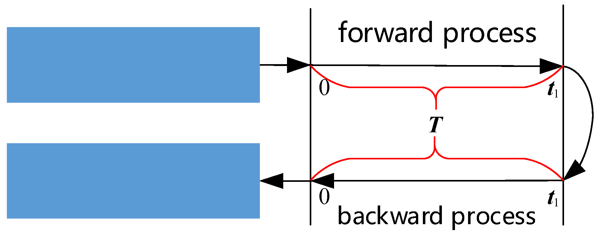
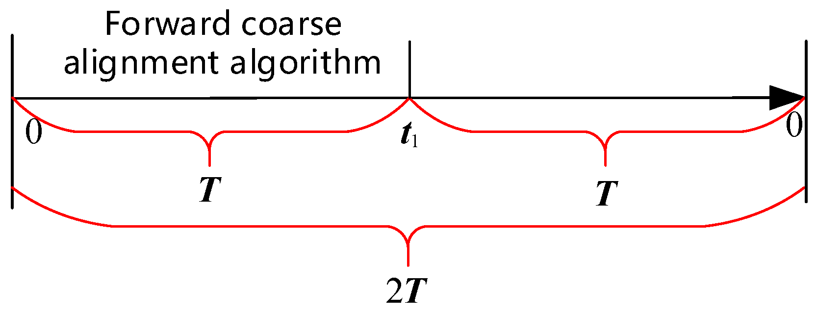
Use the inertial-frame coarse alignment algorithm in Section 2.2 to complete the forward coarse alignment, and store the parameters in $α^{b} (t)$ and $β^{b} (t)$ , gyroscope, accelerometer, and DVL data as the forward data;
Use the partially stored data in the forward process to simulate the data required for the backward coarse alignment process, as detailed in Table 1;
Continue the forward coarse alignment process and use equations (41)-(43) to perform the backward coarse alignment. Finally, the initial attitude matrix $C_{b}^{T} (0)$ can be directly obtained.

3.2. The Polar backtracking fine alignment method

The polar backtracking fine alignment includes three parts in total. The first part is to complete the forward navigation and coarse alignment using the stored forward data, after completing the backtracking coarse alignment. The second part is to simulate and generate the necessary data for the backtracking process using the stored data and complete the backward navigation. The third part is to use the stored forward data to complete the forward navigation and fine alignment under small misalignment, as shown in Figure 4.

The polar integrated fine alignment under large azimuth misalignment is achieved using the algorithm in Section 2.3. The polar integrated alignment under small misalignment is achieved using the algorithm in Section 2.4. The forward navigation algorithm, the backward data simulation generation strategy, and the backward navigation algorithm are shown below.

This paper establishes a transverse inertial forward navigation algorithm based on the transverse inertial mechanics arrangement proposed in Reference [14], and derives the transverse inertial backward navigation algorithm. The attitude, velocity, and position update algorithms for transverse SINS are as follows[14]:

{\dot{C}}_{b}^{T} = C_{b}^{T} (ω_{T b}^{b} \times)

(46)

{\dot{V}}^{T} = C_{b}^{T} f^{b} - (2 ω_{i e_{T}}^{T} + ω_{e_{T} T}^{T}) \times V^{T} + G^{T}

(47)

{\dot{L}}_{T} = - \frac{1}{τ} v_{e}^{T} + \frac{1}{R_{y}} v_{n}^{T}

(48)

{\dot{λ}}_{T} = \frac{1}{R_{x} \cos L_{T}} v_{e}^{T} - \frac{1}{τ \cos L_{T}} v_{n}^{T}

(49)

In the actual execution of the algorithm, it is necessary to discretize Equations (46)–(49) to obtain the corresponding recursive algorithm and define it as the forward navigation algorithm, which is shown below:

\begin{matrix} C_{b, k}^{T} = C_{T (k - 1)}^{T (k)} C_{b, k - 1}^{T} C_{b (k)}^{b (k - 1)} \\ \approx M_{R V} [T_{s} (- ω_{i T, k}^{T})] C_{b, k - 1}^{T} M_{R V} [T_{s} ω_{i b, k}^{b}] \end{matrix}

(50)

V_{k}^{T} = V_{k - 1}^{T} + T_{s} [C_{b, k - 1}^{T} f_{k}^{b} - (2 ω_{i e_{T}, k - 1}^{T} + ω_{e_{T} T, k - 1}^{T}) \times V_{k - 1}^{T} + G^{T}]

(51)

L_{T, k} = L_{T, k - 1} + T_{s} [- \frac{1}{τ_{k - 1}} v_{e, k - 1}^{T} + \frac{1}{R_{y, k - 1}} v_{n, k - 1}^{T}]

(52)

λ_{T, k} = λ_{T, k - 1} + T_{s} [\frac{1}{R_{x, k - 1} \cos L_{T, k - 1}} v_{e, k - 1}^{T} - \frac{1}{τ_{k - 1} \cos L_{T, k - 1}} v_{n, k - 1}^{T}]

(53)

where,

M_{R V} [T_{s} ω] = I + \frac{\sin |T_{s} ω|}{|T_{s} ω|} (T_{s} ω \times) + \frac{1 - \cos |T_{s} ω|}{{|T_{s} ω|}^{2}} {(T_{s} ω \times)}^{2}

(54)

where

k

represents the recursive cycle,

(k = 1, 2, 3...)

T_{s}

is the inertial solving cycles.

C_{T (k - 1)}^{T (k)}

represents the rotation change of frame

T

with respect to the reference frame

i

from time

k

to time

k - 1

, and

C_{b (k)}^{b (k - 1)}

represents the rotation change of frame

b

with respect to the reference frame

i

from time

k - 1

to time

k

The inverse navigation algorithm can be obtained by rearranging Equations (50)–(53) through a series of variable substitutions and algebraic manipulations.

\begin{matrix} C_{b, k - 1}^{T} & = C_{T (k)}^{T (k - 1)} C_{b, k}^{T} C_{b (k - 1)}^{b (k)} \\ \approx M_{R V} [T_{s} ω_{i T, k - 1}^{T}] C_{b, k}^{T} M_{R V} [T_{s} (- ω_{i b, k - 1}^{b})] \end{matrix}

(55)

\begin{matrix} (- V_{k - 1}^{T}) & = (- V_{k}^{T}) + T_{s} [C_{b, k - 1}^{T} f_{k}^{b} - (2 (- ω_{i e_{T}, k - 1}^{T}) + (- ω_{e_{T} T, k - 1}^{T})) \times (- V_{k - 1}^{T}) + G^{T}] \\ \approx (- V_{k}^{T}) + T_{s} [C_{b, k}^{T} f_{k - 1}^{b} - (2 (- ω_{i e_{T}, k}^{T}) + (- ω_{e_{T} T, k}^{T})) \times (- V_{k}^{T}) + G^{T}] \end{matrix}

(56)

\begin{matrix} L_{T, k - 1} = L_{T, k} + T_{s} [- \frac{1}{τ_{k - 1}} (- v_{e, k - 1}^{T}) + \frac{1}{R_{y, k - 1}} (- v_{n, k - 1}^{T})] \\ \approx L_{T, k} + T_{s} [- \frac{1}{τ_{k}} (- v_{e, k}^{T}) + \frac{1}{R_{y, k}} (- v_{n, k}^{T})] \end{matrix}

(57)

\begin{matrix} λ_{T, k - 1} & = λ_{T, k} + T_{s} [\frac{1}{R_{x, k - 1} \cos L_{T, k - 1}} (- v_{e, k - 1}^{T}) - \frac{1}{τ_{k - 1} \cos L_{T, k - 1}} (- v_{n, k - 1}^{T})] \\ \approx λ_{T, k} + T_{s} [\frac{1}{R_{x, k} \cos L_{T, k}} (- v_{e, k}^{T}) - \frac{1}{τ_{k} \cos L_{T, k}} (- v_{n, k}^{T})] \end{matrix}

(58)

Clearly, by comparing (50)–(53) and (55)–(58), it can be seen that to achieve backward navigation, it is only necessary to take the negative of the results of

ω_{i e_{T}}^{T}

ω_{e_{T} T}^{T}

V^{T}

, and

ϕ_{i b}^{b}

. Therefore, the specific method of simulating backward data using the stored data from the forward process is as follows:

Firstly, the stored data of the gyroscope and accelerometer in the forward process are reversed, and then the Earth's rotation angular velocity

ω_{i e}

, gyroscope output angular rate

ω_{i b}^{b}

, and initial velocity for reverse navigation are negated to obtain the simulated reverse data.

In summary, the proposed backtracking fine alignment method consists of the following steps:

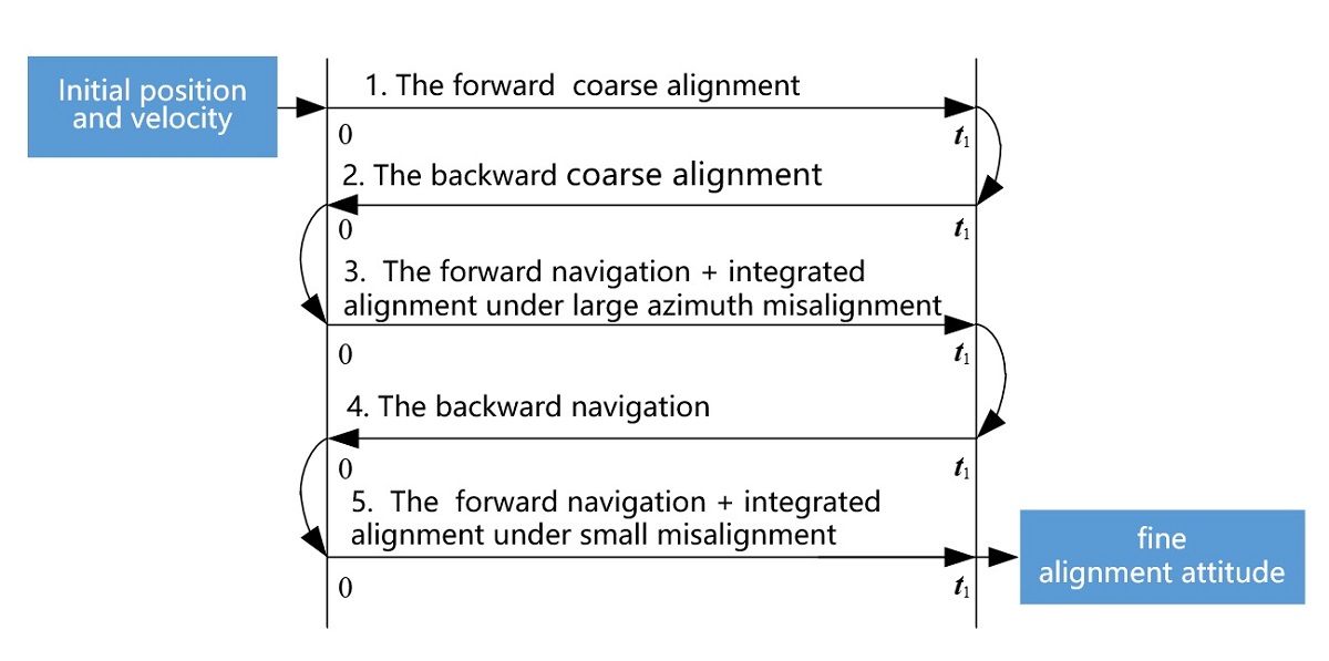
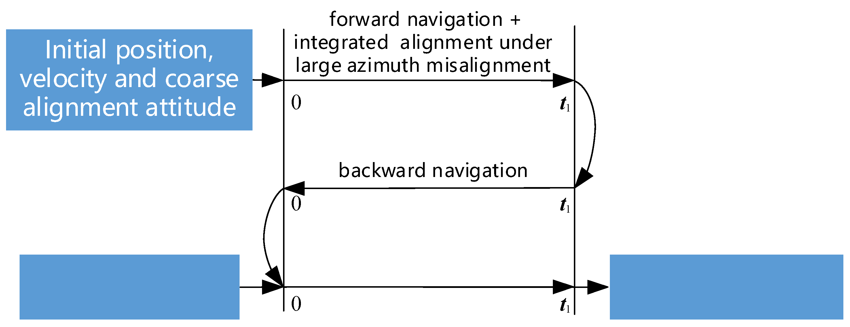
Using Equations (50)–(53) and the algorithm in Section 2.3 to perform forward navigation and achieve the polar integrated fine alignment under the large misalignment;
Utilizing the data required for the backward navigation process generated through forward data simulation, and using the initial navigation parameters estimated for the forward navigation process, which consist of the attitude, velocity, and position at the final time, to perform backward navigation with Equations (55)–(58);
Using the known initial position and velocity at the starting time for the forward navigation process, the attitude obtained from the backward navigation process at the final time is employed as the initial attitude for the forward navigation process. Equations (50)–(53) and the algorithm in Section 2.4 are then used to perform forward navigation and achieve precise alignment of the small misalignment angle combination, resulting in the attitude matrix $C_{b}^{T} (t_{1})$ at the final time and completing the alignment of the dynamic base.

4. Experimental Results and Analysis

In this section, we carry out numerical experiments to evaluate the validity of our algorithm. Limited by the geographical location of the authors' country, far from the Arctic, this paper conducted semi-physical experiments. The definite latitude and longitude determine navigation systems' ideal output, not affected by wherever the carrier is. Thus, the truth value generated by the trajectory generator and the sensor error extracted from SINS and DVL is synthesized to construct the semi-physical experimental data. The experiments are conducted to verify the performance of the inertial-frame coarse alignment algorithm aided by the

V^{b}

based on the transverse Earth model, the polar backtracking coarse alignment algorithm, and the polar backtracking fine alignment algorithm proposed in this paper.

4.1. Semi-physical Experimental Conditions

The inertial measurement unit (IMU), composed of the three-axis gyroscope and accelerometer, provides the measured data of SINS, as shown in Figure 5. The inertial measurement unit is installed on the high-precision turntable, as shown in Figure 6.

The ideal output,

ω_{i b}^{b}

and

f_{i b}^{b}

, can be inverted from the determined trajectory, and IMU outputs the practical

{\hat{ω}}_{i b}^{b}

and

{\hat{f}}_{i b}^{b}

. Thus, the measurement error is

\{\begin{cases} δ ω_{i b}^{b} = {\hat{ω}}_{i b}^{b} - ω_{i b}^{b} \\ δ f_{i b}^{b} = {\hat{f}}_{i b}^{b} - f_{i b}^{b} \end{cases}

(59)

After subtraction, the sensor errors are as follows. The 3-axis gyro constant drift is 6.3895×10^-9rad/s, -4.0947×10^-9rad/s and -1.9605×10^-9rad/s. Its random drift is 3.917×10^-6rad/s, 3.264×10^-6rad/s and 1.534×10^-6rad/s. The 3-axis acceleration constant drift is 5.0024×10^-6m/s², 2.7952×10^-6m/s² and -7.2110×10^-6m/s². Its random drift is 0.00161m/s², 0.001698m/s² and 0.0003726m/s².

The measurement error of DVL-based velocity is extracted from the data resource of the sea trial near Dalian. The trial carries a ship-borne SINS/GNSS integrated navigation system and DVL. The SINS/GNSS integrated navigation system outputs a velocity reference

V

, and DVL outputs the measured velocity

{\hat{V}}_{D V L}^{b}

. Thus, the measurement error of DVL is:

δ V_{D V L}^{b} = {\hat{V}}_{D V L}^{b} - V

(60)

The measurement error of DVL is shown in Figure 7. Due to the interference by the actual environment, the noise contains large gross errors.

To simulate the actual movement of the body in mid-latitude and polar regions, we designed a trajectory for the transverse Earth model, with parameter settings as follows:

(1) The navigation parameters in mid-latitude region

The initial position is

[1 ° N, 50 ° E, 0 m]

(The initial position in the Earth model is

[39.99 ° N, 1.31 ° E, 0 m]

), The transverse eastward and northward errors are both 10m, the initial attitude is

[0 °, 0 °, 60 °]

, the initial velocity is 5m/s;

(2) The navigation parameters in the polar region

The initial position is

[1 ° N, 2 ° E, 0 m]

(The initial position in the Earth model is

[87 . 76 ° N, 26 . 57 ° E, 0 m]

), The transverse eastward and northward errors are both 10m, the initial attitude is

[0 °, 0 °, 60 °]

, the initial velocity is 5m/s.

4.2. Performance verification of the inertial-frame coarse alignment algorithm under transverse Earth model

In order to validate the feasibility of the proposed inertial-frame coarse alignment algorithm under transverse Earth model in Section 2.2, this study employs mid-latitude and polar motion scenarios designed in Section 4.1, and conducts coarse alignment using both the traditional inertial-frame coarse alignment algorithm [11] and the proposed algorithm under the transverse Earth model. The simulation duration is set to 600s, and the experimental results are presented in Figure 8 and Figure 9, as well as Table 2.

Based on the analysis of Figure 8 and Figure 9, and Table 2, it can be observed that the alignment errors of both the traditional inertial-frame coarse alignment algorithm and the proposed algorithm under transverse Earth model gradually decrease with the increase in alignment time in different regions. In the mid-latitude region, the experimental results reveal that both algorithms have similar accuracy at 600s, with attitude errors of less than 1', and can achieve coarse alignment of the moving base. Therefore, the feasibility of the proposed algorithm is verified in this region. In the polar region, the experimental results indicate that both algorithms have a horizontal attitude error of less than 1' at 600 seconds, with transverse azimuth errors of -35.16° and -40.15°, respectively. The proposed algorithm under transverse Earth model exhibits higher azimuth accuracy, with an improvement of 12.43% compared to the traditional inertial-frame coarse alignment algorithm. This improvement is attributed to the fact that the proposed algorithm eliminates the impact of longitude error amplification on the alignment in the polar region.

Additionally, a comparison of Figure 8 and Figure 9 reveals that the horizontal attitude error of both algorithms is not affected by increasing latitude, while the transverse alignment error increases with latitude. This is due to the fact that as the latitude increases, the earth vector and gravity vector tend to be aligned, reducing the coupling effect between the north direction and the azimuth loop, leading to a decrease in transverse alignment capability, while the horizontal attitude alignment capability is not affected. Therefore, in the polar region, although the transverse alignment error of the inertial coarse alignment algorithm under the transverse earth model is smaller than that of the traditional inertial-frame coarse alignment algorithm, it still results in a large alignment error.

4.3. Performance Verification of the polar Backtracking Coarse Alignment Algorithm

To verify the performance of the polar backtracking coarse alignment algorithm presented in Section 3.1, we utilized the polar motion scenario designed in Section 4.1 and performed coarse alignment using both the inertial-frame coarse alignment algorithm under the transverse earth model and the polar backtracking coarse alignment algorithm. The simulation lasted for 180s, and the experimental results are shown in Figure 10 and Table 3. It should be noted that since the backtracking coarse alignment algorithm does not affect the final velocity and position error of the moving base alignment, this section only presents a comparison of the attitude error between the two algorithms and analyzes the attitude accuracy and alignment time of the polar backtracking coarse alignment algorithm.

Based on the results presented in Figure 10 and Table 3, both algorithms achieved horizontal attitude error less than 1' after 180s of semi-physical simulation data. The transverse azimuth error for the inertial-frame coarse alignment algorithm under the transverse Earth model was -59.86°, while that for the polar backtracking coarse alignment algorithm was -35.37°, indicating a 40.91% higher azimuth accuracy for the polar backtracking coarse alignment algorithm than that for the inertial-frame coarse alignment algorithm under transverse Earth model. The experimental results show that both algorithms have small horizontal attitude error, which meets the alignment requirements. The polar backtracking coarse alignment algorithm has smaller transverse azimuth error than the inertial-frame coarse alignment algorithm under transverse Earth model. This is mainly because the inertial-frame coarse alignment algorithm under transverse Earth model requires a longer time to complete the alignment in the polar region, and its alignment result cannot fully converge within 180s, leading to a larger transverse azimuth error. However, the polar backtracking coarse alignment algorithm extends the alignment time, and its alignment result can further converge, resulting in a smaller transverse azimuth error.

Moreover, since the polar motion navigation parameters in section 4.2 are consistent with those in section 4.3, a comprehensive comparison of Table 2 and Table 3 shows that the transverse azimuth error of the inertial-frame coarse alignment algorithm under the transverse earth model at 600s is -35.16°. However, by utilizing semi-physical simulation data with a duration of 180s, the polar backtracking coarse alignment algorithm yields a transverse azimuth error of -35.37°, which is similar to that of the former algorithm. Therefore, employing the polar backtracking coarse alignment algorithm can effectively save alignment time, while the alignment accuracy is not compromised.

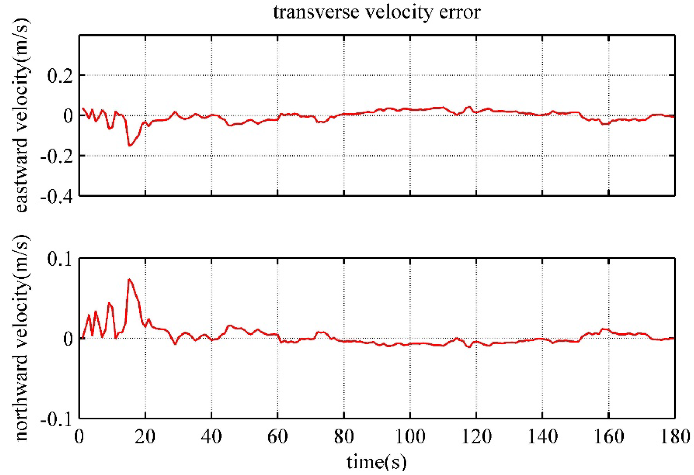
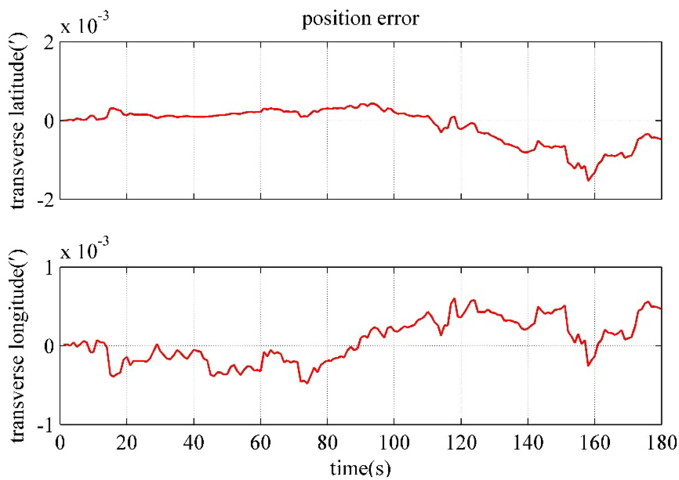
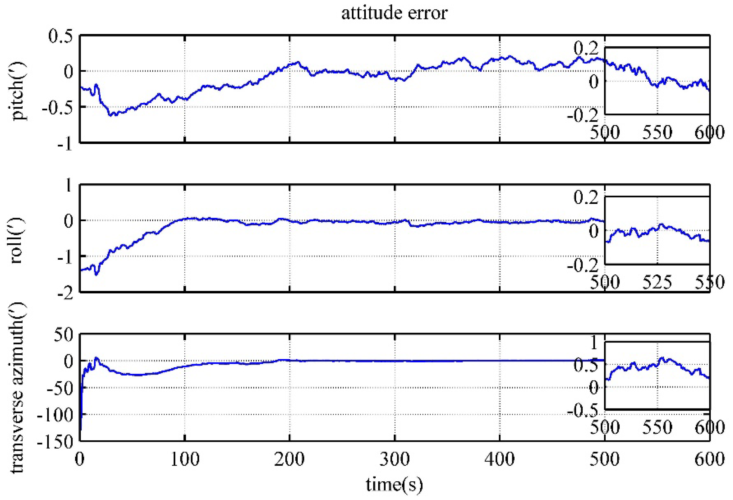
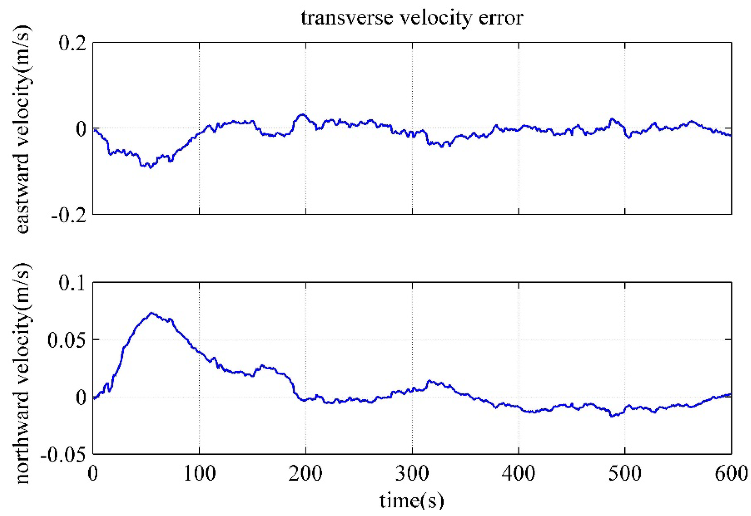
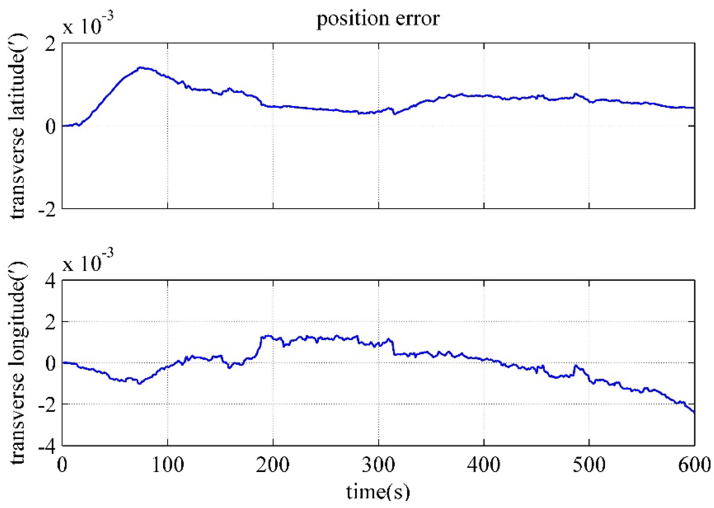
4.4. Performance Verification of the polar Backtracking Fine Alignment Algorithm

According to reference [18], The polar integrated fine alignment under large azimuth misalignment can complete alignment in 600s. To verify the performance of the polar backtracking fine alignment algorithm proposed in section 3.2, we simulated the polar motion scenario designed in section 4.1. Then we compared the attitude, velocity, and position errors at the end of alignment using the backtracking fine alignment algorithm and the integrated fine alignment under large azimuth misalignment in section 2.3 for 180s and 600s, respectively, after simulating 180s with the backtracking coarse alignment algorithm. The results are shown in Figure 11, Figure 12, Figure 13, Figure 14, Figure 15, Figure 16, Figure 17 and Figure 18 and Table 4. It should be noted that, according to the backtracking fine alignment steps in section 3.2, the backtracking fine alignment algorithm will use the known initial velocity and position to correct the inertial velocity and position after inverse navigation. Therefore, to obtain the velocity and position errors of the backtracking fine alignment algorithm, only the simulation results of step 3 need to be presented, as shown in Figure 12 and Figure 13.

According to Figure 11, Figure 12, Figure 13, Figure 14 and Figure 15 and Table 4, the polar integrated fine alignment under large azimuth misalignment achieves a transverse attitude error of less than 1' and a transverse azimuth error of -3.502' at 180s. The attitude errors for the polar backtracking fine alignment algorithm are also less than 1'. The transverse azimuth error is significantly improved by 73.59%. This is due to the fact that the alignment time is short and the filtering of the polar integrated fine alignment algorithm under large azimuth misalignment has not fully converged yet. At 600s, the polar integrated fine alignment algorithm also achieves an attitude error of less than 1', which meets the alignment requirements for the polar region. The difference in transverse velocity errors between the two algorithms is not significant, mainly because both algorithms can obtain the body velocity provided by the DVL. When the attitude error is small, the DVL velocity can be converted into transverse velocity with small error and provided to the integrated alignment system. At both 180s and 600s, the attitude errors for both algorithms are relatively small, which results in similar transverse velocities. However, at 600s, the position error of the polar integrated fine alignment algorithm is larger than that of the integrated alignment algorithm under large azimuth misalignment. This is because the observability of the position of the integrated alignment system is poor when only the body velocity is available for assistance, and the position error gradually accumulates as the alignment time increases. Overall, compared with the integrated alignment algorithm under large azimuth misalignment, the Polar backtracking fine alignment algorithm not only has smaller positioning errors, but also requires less alignment time, which is 70% less than that of the integrated precision alignment algorithm under large azimuth misalignment.

5. Conclusion

In this study, we proposed a polar moving base alignment method based on backtracking scheme to achieve fast and high-precision alignment in the polar region. Firstly, a polar coarse alignment algorithm in the inertial frame under the transverse Earth model is designed to eliminate the effect of the alignment algorithm caused by longitude error amplification. Then, the polar coarse and fine alignment methods based on backtracking scheme are designed respectively. In the coarse alignment, the data storage scheme was optimized to reduce the computational burden. In the fine alignment, we derive the forward and backward navigation algorithms for transverse SINS suitable for polar regions. We design a backtracking scheme that combines the alignment with large azimuth misalignment and small misalignment, which ensures alignment accuracy and reduces alignment time. The results of semi-physical simulation experiments show that, compared with previous methods, the coarse alignment algorithm in the inertial frame under the transverse Earth model has increased the azimuth accuracy by 12.43%, the retrograde coarse alignment algorithm has increased the azimuth accuracy by 40.91%, and the retrograde fine alignment method has increased the azimuth accuracy by 73.59%. The algorithm proposed in this paper has a promising application prospect in the polar region.

Author Contributions

Conceptualization, J.L. and J.C.; methodology, J.L.; validation, J.L.; formal analysis, J.L.; writing—original draft preparation, J.L.; writing—review and editing, Y.W and J.C. All authors have read and agreed to the published version of the manuscript.

Funding

This research was funded by the National Natural Science Foundation of China under Grant 62073093 and Grant 62003108, in part by the Science Fund for Distinguished Young Scholars of Heilongjiang Province under Grant JC2018019, and in part by the Basic Scientific Research Fund under Grant 3072020CFT0403.

Data Availability Statement

Not applicable.

Conflicts of Interest

The authors declare no conflict of interest.

References

Berkman, P.A.; Vylegzhanin, A. N. Environmental security in the Arctic Ocean. Springer, 2012.
Cheng, J.; Liu, J.; Zhao, L. Survey on polar marine navigation and positioning system. Chinese Journal of Ship Research. 2021, 16, 16–29.
Zhou, J.; Nie, X.; Lin, J. A novel laser doppler velocimeter and its integrated navigation system with strapdown inertial navigation. Opt. Laser Technol. 2014, 64, 319–323.
Yao, Y.; Xu, X.; Zhang, T.; Hu, G. An improved initial alignment method for sins/gps integration with vectors subtraction. IEEE Sens. J. 2021, 21, 18256–18262.
Liu, M.; Li, G.; Gao, Y. Improved polar inertial navigation algorithm based on pseudo INS mechanization. Aerosp. Sci. Technol. 2018, 77, 105-116.
Cai, J.; Cheng J.; Zhong, S.; An Innovative Polar Rapid Transfer Alignment Aided by Doppler Velocity Log For Marine Vessels. In Proceedings of the 2019 European Navigation Conference, Warsaw, Poland, 09-12 April 2019.
Luo, L.; Huang, Y.; Zhang, Z.; Zhang, Y. A New Kalman Filter-Based In-Motion Initial Alignment Method for DVL-Aided Low-Cost SINS. IEEE Trans. Veh. Technol. 2021, 70, 331–343.
Xu, X.; Guo, Z.; Yao, Y.; Zhang, T. Robust Initial Alignment for SINS/DVL Based on Reconstructed Observation Vectors. IEEE/ASME Trans. Mechatron. 2020, 25,1659–1667.
Pei, F.; Yang, S.; Yin, S. In-Motion Initial Alignment Using State-Dependent Extended Kalman Filter for Strapdown Inertial Navigation System. IEEE Trans. Instrum. Meas. 2021, 70, 1–12.
Zhang, Q.; Li, S.; Xu, Z. Velocity-based optimization-based alignment (VBOBA) of low-end MEMS IMU/GNSS for low dynamic applications. IEEE Sens. J. 2020, 20, 5527–5539.
Xu, J.; He, H.; Qin, F. A novel autonomous initial alignment method for strapdown inertial navigation system. IEEE Trans. Instrum. Meas, 2017, 66, 2274-2282.
Ouyang, W.; Wu, Y. Optimization-based strapdown attitude alignment for high-accuracy systems: covariance analysis with applications. IEEE Trans. Aerosp. Electron. Syst. 2022, 58, 4053-4069.
Li, Y.; Liu, M.; Gong, J. Double-velocity inertial-frame alignment algorithm with pseudo INS modeling in polar regions. J. Syst. Eng. Electron. 2022, 44, 1677-1684.
Yao, Y.; Xu, X.; Li, Y.; Liu, Y.; Sun, J. Transverse navigation under the ellipsoidal earth model and its performance in both polar and non-polar areas. J. Navig. 2016, 69, 335–352.
Cai, J.; Cheng, J.; Liu, J.; Wang, Z.; Xu, Y. A polar rapid transfer alignment assisted by the improved polarized-light navigation. IEEE Sens. J. 2022, 22, 2508–2517.
Wu, Y.; He, C.; Liu, G.; On inertial navigation and attitude initialization in polar areas. Satell. Navigat. 2020, 1, 1–6.
Liu, J.; Zhao, L.; Qi, B.; Cheng, J.; Cai, J.; A new polar integrated alignment algorithm with the aids of DVL and the improved polarized-light navigation. In Proceedings of the Name of the 5th Int. Symp. Auto. Syst. (ISAS), Hangzhou, China, 08-10 April 2022.
Yan, Z.; Wang, L.; Wang, T.; Zhang, H.; Yang, Z. Polar transversal initial alignment algorithm for UUV with a large misalignment angle. Sensors 2018, 18, 3231.
Cheng, J.; Liu, J.; Cai, J.; and Xu, Y. A Polar Integrated Alignment Assisted by DVL Under Large Azimuth Misalignment. in IEEE Sens. J. 2023, 23, 5962-5973.
Wen, Z.; Yang, G.; Cai, Q. Odometer aided SINS in-motion alignment method based on backtracking scheme for large misalignment angles. IEEE Access, 2020, 7937-7948.
Sun, Y.; Yang, G.; Cai, Q. A robust in-motion attitude alignment method for odometer-aided strapdown inertial navigation system. Rev. Sci. Instrum. 2020, 91.
Wang, D.S.; He, G.Y.; Jiang, X.H. In-motion Alignment Scheme Based on Reverse Kalman Filter. J. Chin. Inertial Technol. 2020, 28, 721–728.
Lin, Y.; Miao, L.; Zhou, Z. A high-accuracy initial alignment method based on backtracking process for strapdown inertial navigation system. Measurement, 2022, 201.
Wahba, G. A least squares estimate of satellite attitude. SIAM Rev. 1965, 7, 409.
Yan, G.; Chen, R.; Guo, K. Equivalence analysis between SVD and QUEST for multi-vector attitude determination. J. Chin. Inertial Technol. 2019, 27, 568-572.

Figure 1. The transverse ellipsoid Earth model.

Figure 2. Timing arrangement of the polar backtracking coarse alignment.

Figure 3. The Running Process of the Polar Backtracking Coarse Alignment.

Figure 4. Timing arrangement of the polar backtracking fine alignment.

Figure 5. Inertial measurement unit.

Figure 6. High-precision three-axis turntable with SINS.

Figure 7. The measurement error of DVL.

Figure 8. Performance comparison of inertial-frame coarse alignment algorithm in mid-latitude region.

Figure 9. Performance comparison of inertial-frame coarse alignment algorithm in polar region.

Figure 10. Comparison of attitude errors between two algorithms.

Figure 11. The attitude error of polar backtracking fine alignment algorithm.

Figure 12. The velocity error of the polar backtracking fine alignment algorithm.

Figure 13. The position error of the polar backtracking fine alignment algorithm.

Figure 14. The attitude error of the polar integrated fine alignment algorithm under large azimuth misalignment.

Figure 15. The velocity error of the polar integrated fine alignment algorithm under large azimuth misalignment.

Figure 16. The position error of the polar integrated fine alignment algorithm under large azimuth misalignment.

Table 1. Data sequence of the polar backtracking coarse alignment.

Initialization	the forward process
0	1	…	$T - 1$	$T$	$T + 1$	…	$2 T - 1$	$2 T$
$C_{b}^{i_{b 0}} (0)$	$C_{b}^{i_{b 0}} (1)$	…	$C_{b}^{i_{b 0}} (t_{1} - 1)$	$C_{b}^{i_{b 0}} (t_{1})$	$C_{b}^{i_{b 0}} (t_{1} - 1) B$	…	$C_{b}^{i_{b 0}} (1) B$	$C_{b}^{i_{b 0}} (0) B$
$V^{b} (0)$	$V^{b} (1)$	…	$V^{b} (t_{1} - 1)$	$V^{b} (t_{1})$	$V^{b} (t_{1} - 1)$	…	$V^{b} (1)$	$V^{b} (0)$
$f^{b} (0)$	$f^{b} (1)$	…	$f^{b} (t_{1} - 1)$	$f^{b} (t_{1})$	$f^{b} (t_{1} - 1)$	…	$f^{b} (1)$	$f^{b} (0)$
$C_{T}^{i_{T 0}} (0)$	$C_{T}^{i_{T 0}} (1)$	…	$C_{T}^{i_{T 0}} (t_{1} - 1)$	$C_{T}^{i_{T 0}} (t_{1})$	$C_{T}^{i_{T 0}} (t_{1} - 1)$	…	$C_{T}^{i_{T 0}} (1)$	$C_{T}^{i_{T 0}} (0)$

Table 2. Coarse alignment results of different inertial-frame coarse alignment algorithms with simulation duration of 600s.

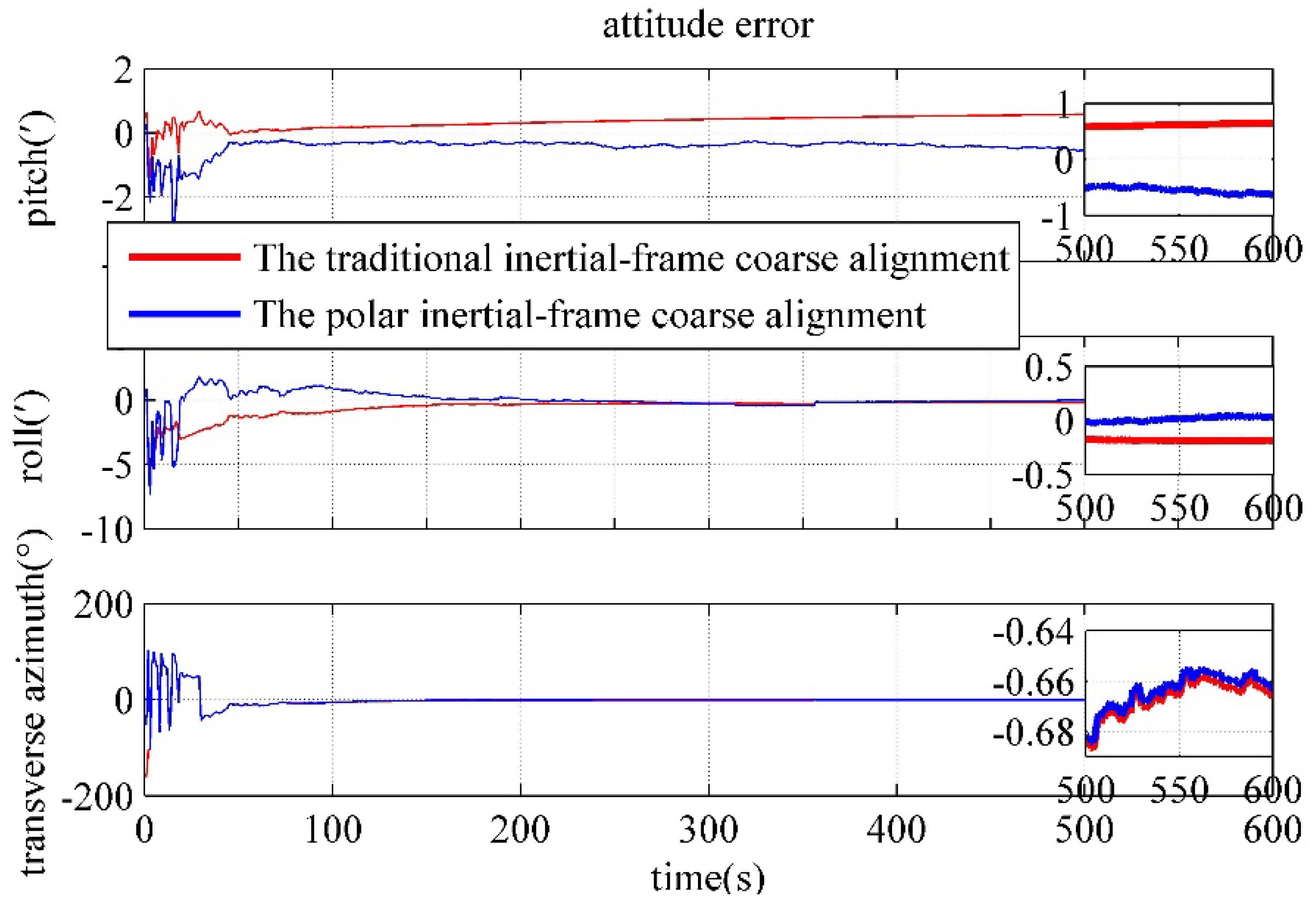
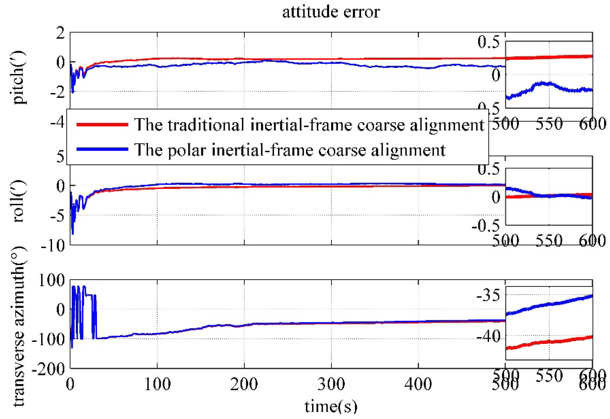
Algorithm	Estimation error	Mid-latitude	Polar
The polar inertial-frame coarse alignment based on the transverse Earth model	Pitch/(')	-0.6292	-0.2342
	Roll/(')	0.0323	-0.0256
	Transverse azimuth/(°)	-0.6614	-35.16
The traditional inertial-frame coarse alignment	Pitch/(')	0.6503	0.2747
	Roll/(')	-0.1848	-0.0372
	Transverse azimuth/(°)	-0.6665	-40.15

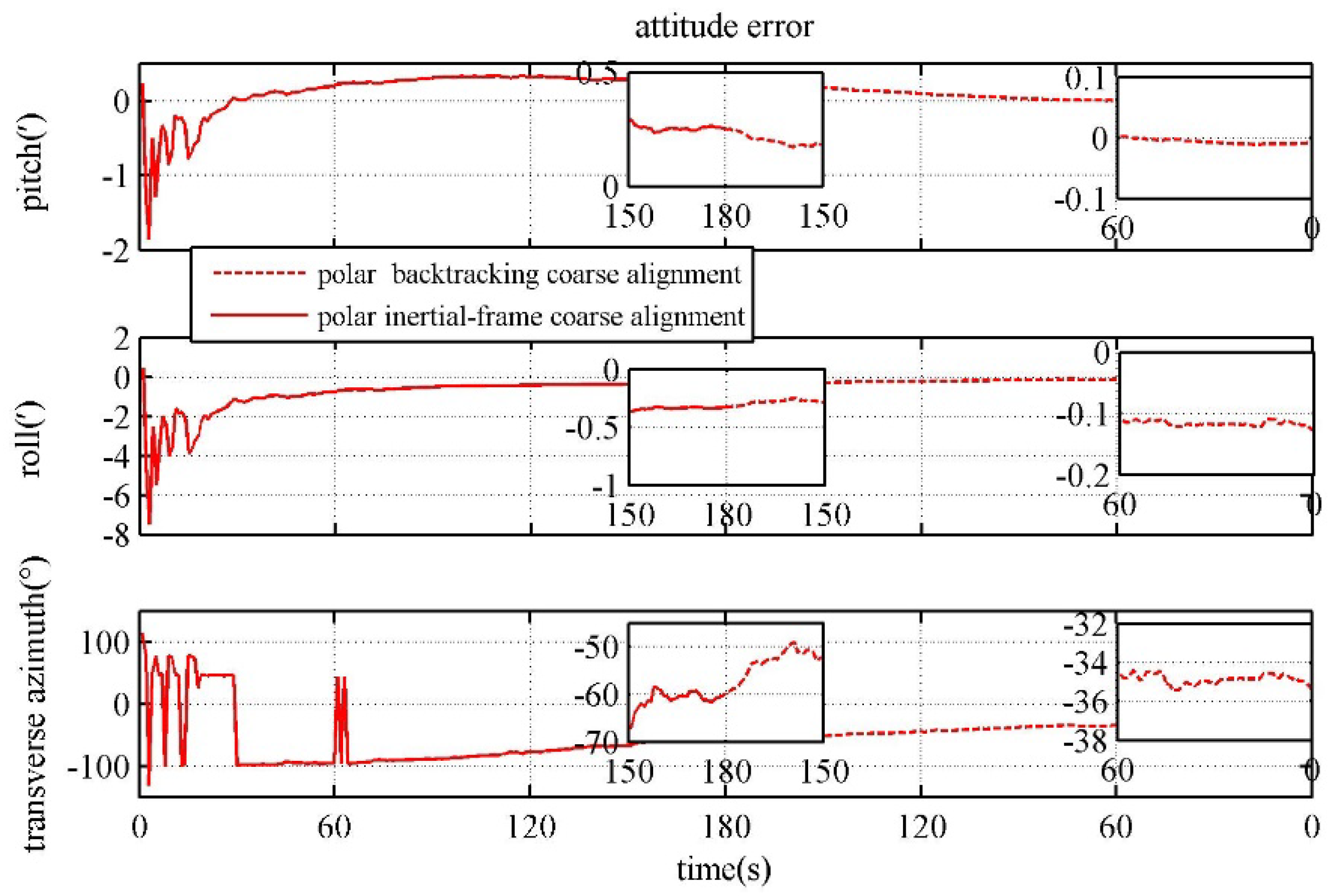
Table 3. Alignment results of two coarse alignment algorithms.

Algorithm	Pitch/(')	Roll/(')	Transverse azimuth/(°)
The inertial-frame coarse alignment based on the transverse Earth model	0.2522	-0.3251	-59.86
The polar backtracking coarse alignment	-0.0084	-0.1285	-35.37

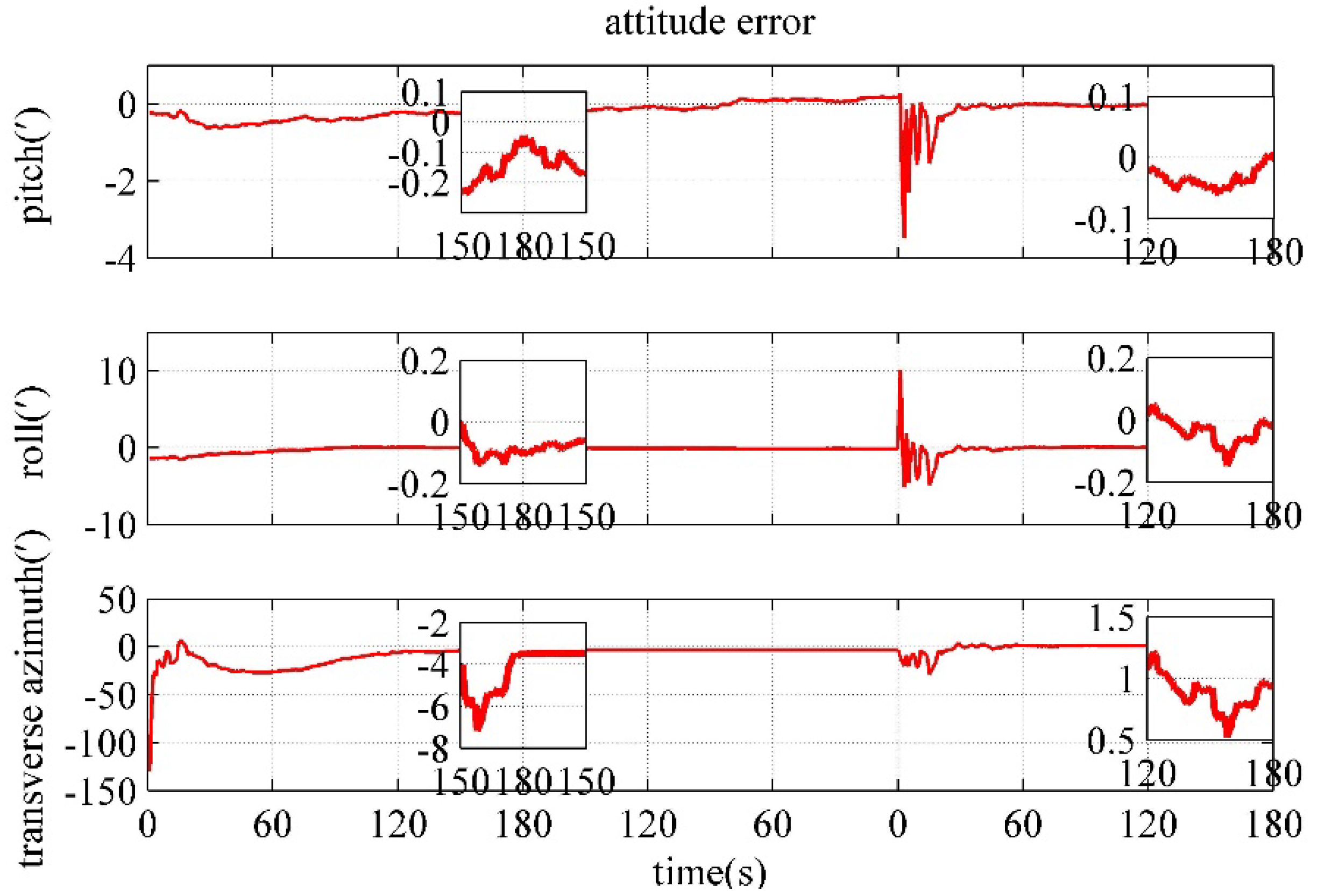
Table 4. Alignment results of two precise alignment algorithms.

Algorithm	The polar backtracking fine alignment	The polar integrated $$$fine alignment
Alignment time/(s)	180	180	600
Pitch error/(')	0.0072	-0.0466	-0.0662
Roll error/(')	-0.0230	-0.1081	-0.0700
Transverse azimuth error/(')	0.9251	-3.502	0.1408
Transverse eastward velocity error/(m/s)	-8.400×10^-3	-0.0189	-0.0184
Transverse northward velocity error/(m/s)	2.879×10^-4	-0.0200	0.0029
Transverse latitude error/(')	4.765×10^-4	7.284×10^-4	4.297×10^-4
Transverse longitude error/(')	4.628×10^-4	1.844×10^-4	2.464×10^-3

Disclaimer/Publisher’s Note: The statements, opinions and data contained in all publications are solely those of the individual author(s) and contributor(s) and not of MDPI and/or the editor(s). MDPI and/or the editor(s) disclaim responsibility for any injury to people or property resulting from any ideas, methods, instructions or products referred to in the content.

© 2023 by the authors. Licensee MDPI, Basel, Switzerland. This article is an open access article distributed under the terms and conditions of the Creative Commons Attribution (CC BY) license (http://creativecommons.org/licenses/by/4.0/).

Copyright: This open access article is published under a Creative Commons CC BY 4.0 license, which permit the free download, distribution, and reuse, provided that the author and preprint are cited in any reuse.

MDPI Initiatives

Important Links

Choose an area of interest and we will send you notifications of new preprints at your preferred frequency.

Disclaimer

A Polar Moving-Base Alignment Based on Backtracking Scheme

Abstract

1. Introduction

2. The Polar Coarse and Fine Alignment Methods

2.1 Transverse Earth Model and the Definition of Transverse Frame

2.2. The inertial-frame coarse alignment algorithm aided by the V b based on the transverse Earth model.

2.3. The polar Fine Alignment Method assisted by DVL under Large Azimuth Misalignment

2.4. The polar Fine Alignment Method assisted by DVL under small misalignment

3. The Polar backtracking alignment method

3.1. The Polar backtracking coarse alignment method

3.2. The Polar backtracking fine alignment method

4. Experimental Results and Analysis

4.1. Semi-physical Experimental Conditions

4.2. Performance verification of the inertial-frame coarse alignment algorithm under transverse Earth model

4.3. Performance Verification of the polar Backtracking Coarse Alignment Algorithm

4.4. Performance Verification of the polar Backtracking Fine Alignment Algorithm

5. Conclusion

Author Contributions

Funding

Data Availability Statement

Conflicts of Interest

References

MDPI Initiatives

Important Links

Subscribe

2.2. The inertial-frame coarse alignment algorithm aided by the $V^{b}$ based on the transverse Earth model.