Preprint

Article

Oriented Crossover in Genetic Algorithms for Computer Networks Optimization

Altmetrics

Downloads

126

Views

Comments

A peer-reviewed article of this preprint also exists.

This version is not peer-reviewed

Submitted:

10 April 2023

Posted:

11 April 2023

You are already at the latest version

Alerts

Abstract

Optimization using Genetic Algorithms (GA) is a well-known strategy in several scientific disciplines. The crossover is an essential operator of the Genetic Algorithm. It has been an active area of research to develop sustainable forms for this operand. In this work, a new crossover operand is proposed. This operand depends on giving an elicited description for the chromosome with a new structure for alleles of the parents. It is suggested that each allele has two attitudes, one attitude differs contrastingly with the other, and both of them complement the allele. Thus, in case of one attitude is good, the other should be bad. This is suitable for many systems which contain admired parameters and unadmired parameters. The proposed crossover would improve the desired attitudes and damp the undesired attitudes. The proposed crossover can be achieved in two stages: the first stage is a mating method for both attitudes in one parent to improving one attitude at the expense of the other. The second stage comes after the first improvement stage for mating between different parents. Hence, two concurrent steps for improvement would be applied. Simulation experiments for the system shows improvement in the fitness function. The proposed crossover could be helpful in different fields, especially to optimize routing algorithms and network protocols, an application that has been tested as a case study in this work.

Keywords:

Subject: Computer Science and Mathematics - Computer Networks and Communications

1. Introduction

A genetic algorithm is a formula for resolving optimization issues that incorporate a constraint and natural selection similar to the biological process that propels evolution. The recent addition of Genetic Algorithm (GA) to Artificial Intelligence was motivated by the biological behavior of chromosomes [1]. 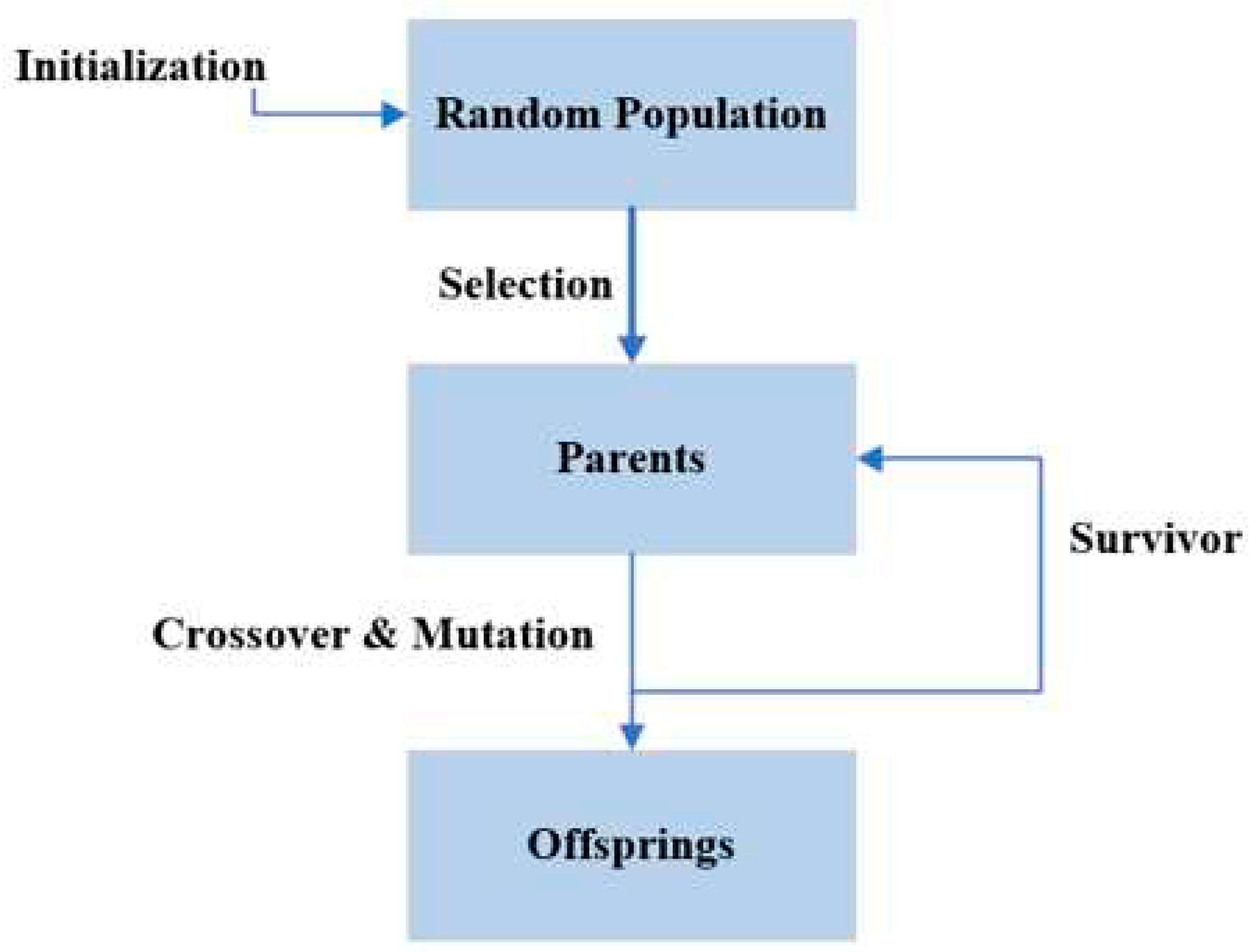The Darwinian evaluation principle known as "Survival of the fittest" is what the Evolution algorithms do [1]. Therefore, the goal of employing GA is to produce the best offspring (solution), which increases the necessity of adopting it. The GA begins with two parents and mates them to generate new offspring; this mating is termed the "crossover." then the old population is replaced with the new one by using the crossover and mutation operators. This process continues until the convergence condition is met [2].

1.1. GA Operands

There are three operands [3] in a typical GA, and they are as follows.

Selection: This operand determines which chromosomes of the population are selected for reproduction. As a chromosome fits better, it is more likely to be selected for reproduction.
Crossover: This operator exchanges the subsequences between two chromosomes before and after a locus that is randomly chosen to create two offspring [3].
Mutation: This procedure involves flipping one or more randomly selected bits in the parent's chromosomes to create offspring from a single parent [4]. Any bit has a slight chance of mutating, like 0.001[3]. The layout shown in Figure 1 represents the typical GA process design.

This approach is based on the observation that specific chromosomally encoded traits are shared by individuals and can be passed to )inherited by( their offspring through crossover [5]. The genes of either one parent or both parents, with mutations, are shared by two offspring.

1.2. Single–Point Crossover

The most well-known and frequently applied crossover model so far among researchers is that presented by Holland John [6]. A crossover site is randomly selected along the length of the matched strings, and bits immediately near the cross-sites are exchanged.

The beneficial traits of the parents may be combined to produce better offspring when the right site is chosen. If the right place is selected when good parents are mated, the offspring will be better; if not, the string quality will be severely hampered. If the head and tail of one chromosome contain acceptable genetic material, then no offspring will acquire the two beneficial traits straight after the single-point crossover.

1.3. N-Point Crossover

De Jong [7] was the first to use the n-point crossover. it was the same for single-point crossover. In a two-point crossover, there are two relevant crossing sites. The performance of genetic algorithms can be severely continual impacted by the interruptions of building blocks caused by the continual addition of crossover sites.

1.4. Uniform Crossover

Gilbert presented a uniform crossover[8], here, the chromosomes are not broken up by uniform crossover for recombination, since each gene in a child's offspring is made by copying it from a parent who has been selected based on the bit that corresponds to it in a binary crossover mask that is the same length as the parent chromosomes. The two parents are chosen for crossover through the uniform crossover, it produces two children with n genes uniformly chosen from both parents. A random real integer determines whether the first child chooses the i^th genes from the first or second parent [9].

1.5. Numerical Chromosome Representation

The crossover mostly used the binary encoded chromosomes and for real-value encoding, the numerical crossover is utilized. Here, two parent chromosomes are combined linearly by the numerical crossover operator. Two chromosomes are randomly chosen for crossover, resulting in two children who are a linear blend of their parents. N-point is mainly used in the case of binary encoded chromosomes [1].

1.6. Operators Definition

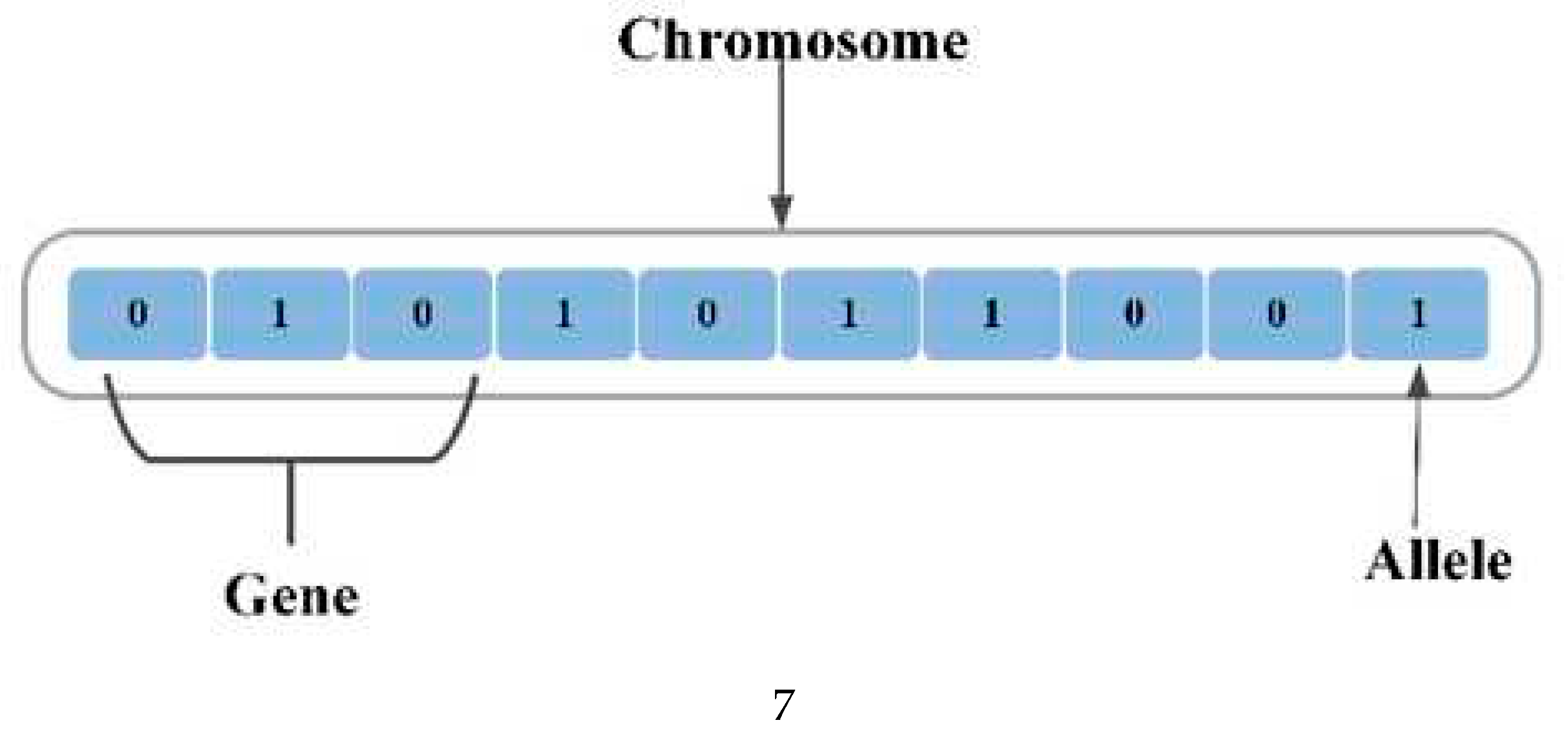
Numerous operators mention the main parts of a genetic algorithm form; A gene is a string of (bit or real number) within a specific length; a chromosome is a term used to describe a sequence of genes. An allele, which can be represented by a symbol or bit, is the smallest chromosomal unit. While a phenotype offers an external description of the individual, a genotype is a piece of data contained in a chromosome [4,10]. The main operand of GA is depicted in Figure 2.

In this article, a new construction proposed for the allele, where supposed that each allele in the chromosome contain two attitudes, one good and the other is bad, add to that a new optimization method has been presented to improve the good or preferred attitude on the cost of unpreferred one. The new optimization method come from changing in the core of Genetic algorithm. Thus, the proposed method can apply with any system specially in computer network optimization.

2. Related Works

2.1. Original Theories

Gilbert Syswerda [8] was first to present the uniform crossover for GA, even at the one point, the second point was presented, but the uniform crossover showed its outperform in optimization, and till now, this crossover type is applicable in many different science fields.

William M. Spears [7] presented an adaptive algorithm to decide when a particular crossover(one point, second point, or uniform) will be optimal for any problem. However, it still, work with standard crossover.

Umbarkar et all [9] presented an excellent review showing more than thirty-five types of crossover presented till 2015, all the suggested researches used in different optimization fields.

Chiroma Haruna et all, [4] presented a review that show the importance of GA in optimization for Machine Learning and Deep learning.

A schema that included the two-point crossover was published by Abid Hussain et all [2], where the proposed methods offer a contrastive convergence rate.

When the balance between the traits of parents and offspring was a challenge in GA optimization, Luca Manzoni et all [5] presented balanced crossover operators that guarantee the offspring has the same balanced features as the parents.

[4] presented a modified optimization method depending on AI. Presented guidance for both beginner and experienced researchers designing evolutionary neural networks, assisting them in selecting appropriate genetic algorithm operator values for use in applications in a certain issue domain.

2.2. Implementation of GA

Various research work has been published on (GA); the latest work carried out by researchers have been discussed here in this section. A genetic algorithm was used in the model presented by Nicolas Kirchner-Bossi and Fernando Porté-Agel [11] to reduce the power losses caused by turbine wakes in wind farms.

A new flight trajectory computation made with (GA) was proposed by Félix Patrón, Roberto Salvador Botez, and Ruxandra Mihaela [12]. The approach examined lateral and vertical navigation to determine the most fuel-efficient cruise trajectory, with optimization by GA saving up to 5.6% in gasoline.

Dana Bani-Hani, Naseem Khan, Fatimah Alsultan, Shreya Karanjkar, and Nagen Nagarur [13] used deep learning’s convolutional neural network to classify four types of leucocytes. A genetic algorithm was used to optimize the CNN's hyperparameters (GA); this article showed that CNN is not efficient in getting optimal.

Fatemeh Ahmadi Zeidabadi, and Mohammad Dehghani [14] presented a new optimization method called Puzzle Optimization Algorithm(POA), which can be used in different optimization problems. The advantage of this method is that there are no control parameters, thus not requiring parameter sitting.

Khandelwal Anju, Kumar Avanish [15] presented a technique based on fuzzy triangular numbers that have been applied to the recruitment process of the individual to the employee. Moreover, the genetic algorithm used for optimization, where the author presented a solving for the selection process to the individual through GA and fuzzy ranking.

Safira Begum, Sunita S Padmannavar[16] they used ensemble classifiers to present a student predictive model and pre-pressing to implement their search before classifying utilizing data mining methodology in their research on educational data mining (EDM). The best solution was then discovered, and GA was utilized to look for issues and raise the likelihood that they would be resolved.

Haldulakar Rupali ,Agrawal Jitendra [17] offered an innovative way in strong rule generation, one of the key components of data mining, where the author employed it differently to construct rules. However, the best optimization technique for generating rules was the genetic algorithm.

Shatha Abdulhadi Muthana and Ku Ruhana Ku-Mahamud [18] To determine the optimal choice for scheduling generator maintenance, various multi-objective optimization methods were examined. One optimization method, Non-dominated Sorting Genetic Algorithm, exemplifies the importance of utilizing GA and optimization in a variety of scientific fields.

Furkan Rabee et all [19] present a new crossover operand for the genetic algorithm called Quarterly crossover (QC), by assuming a different structure for genes within the chromosome which results in two crossovers intended to be an optimization solution for real-time scheduling. Project related for this paper as expanded optimization tools and parameters for network.

2.3. Optimization in Fields of Science

The field of cloud computing improvement and WSN is getting a lot of attention among other fields, where the energy consumption of nodes in the network should be restricted. Therefore, Singh J. [21] used the optimization technique to reduce the utilization of the energy of the data center in the way to accomplish the quality of service.

[22,23,24] presented an energy-efficient deployment method for sensor nodes by clustering the nodes and applying the optimization technique for optimal reduction of the nodes' battery. The optimization for nodes led to the optimization routing protocol. Paolo Cinat et all [25], depending on GA in Mechanical engineering, used in multi-scale surface roughness, presented three genetic algorithms to superimpose and merge the mathematical description of chromosomes to determine the best roughness features.

3. Area of the Proposed Work

The main goal of network optimization is to reduce the problems that occur in any network, to get performance at the lowest possible cost. The network must promote increased throughput and usability and allow data to flow effectively and efficiently. This is accomplished by managing network latency, traffic volume, network bandwidth, and traffic direction [26].

3.1. Applications of the Proposed Work

The proposed work in this article supposes to be for many applications in the field of optimization, such as Computer networks, Routing algorithms, wireless sensor networks … etc. Our interest in this paper will be routing algorithms, where efficiently routing packets through nodes is very important because it will find the path between two entities (two nodes) with the least amount of disturbance [20]. The proposed modification to the genetic algorithm improves the distance, where this proposed method differs from others in that it takes into account network congestion when optimizing.

3.2. Minimal-Cost Network Flow

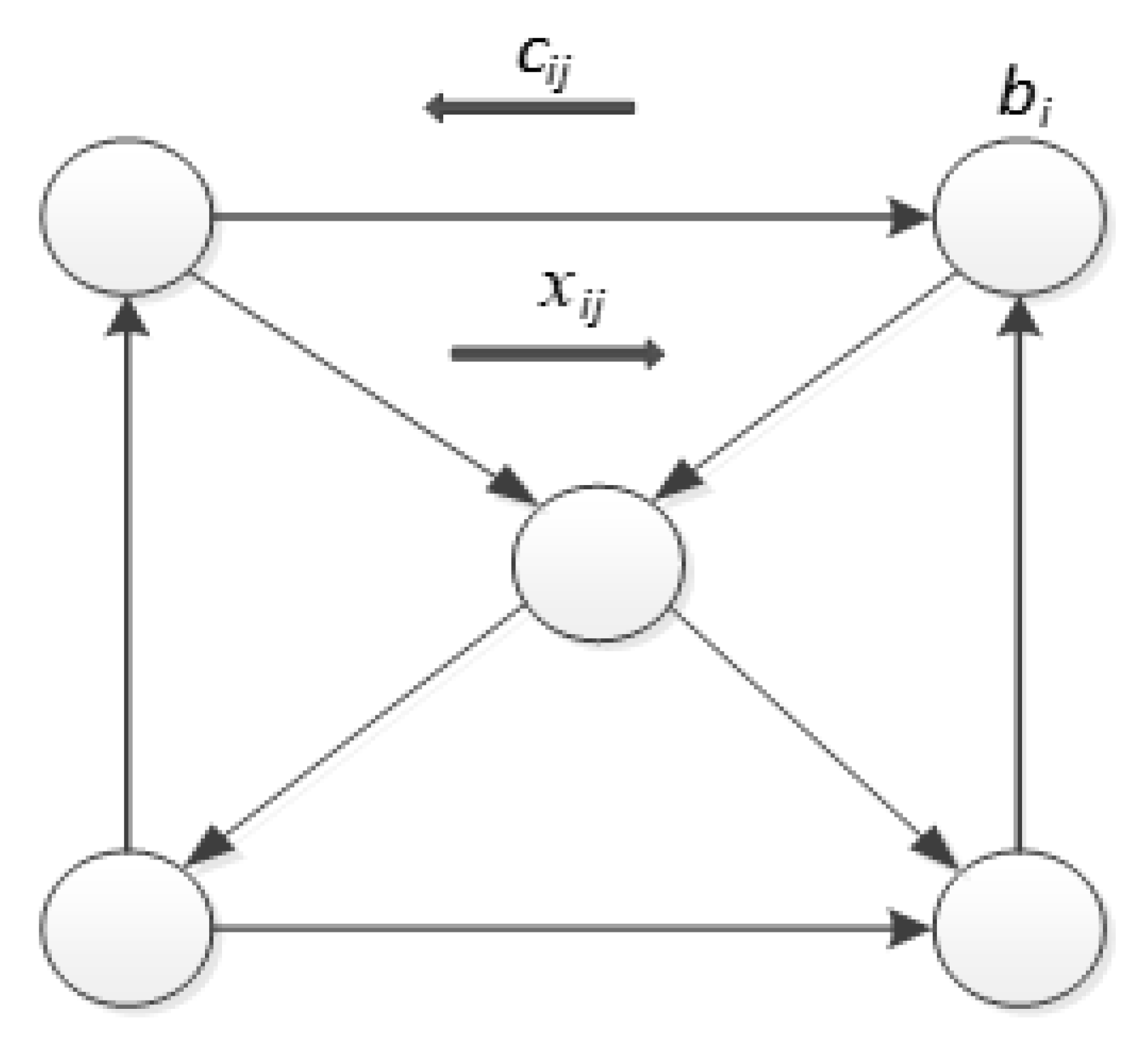
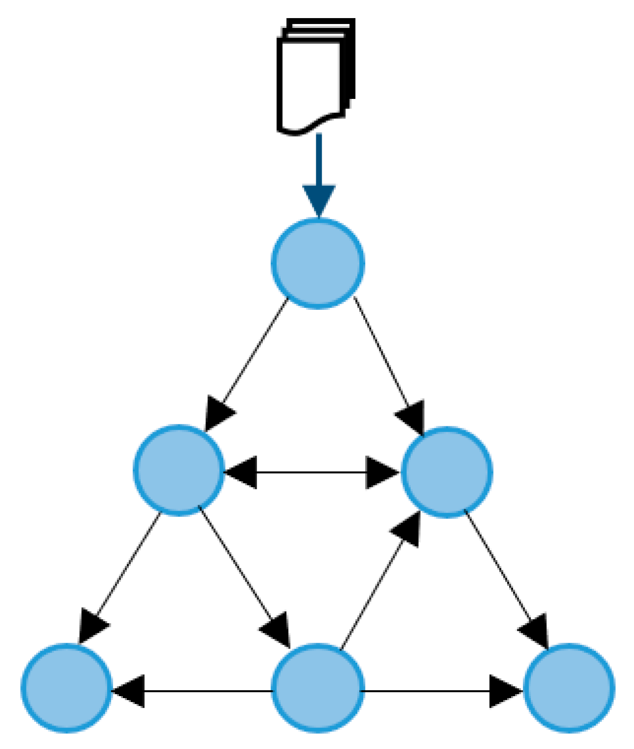
The minimal-cost network-flow problem deals with a single commodity that must be distributed over a network [27]. Suppose there is a network with five nodes, as shown in Figure 3, the minimal-cost network-flow problem deals with a single commodity that must be distributed over a network. Consider a directed graph G=(N,A) with the set of nodes N and the set of links A. The cost of sending a unit flow on link (i,j)

\in

A is c_ij, also x_ij, which is the amount of flow on link (i,j).

We first define b_i

\forall

i∈N, where b_i denotes the amount of supply for source nodes and b_i>0, on the other hand b_i<0 denotes the demand size for sink nodes. Also, b_i=0 will be for intermediate nodes. For simplicity we assume

\sum_{i \in N} b_{i} = 0

, which can be relaxed easily.

The minimal cost of such a problem to optimize in Eq. (1) [27].

z = \sum_{(i, j) \in A} c_{i j} x_{i j}

(1)

There may be upper bounds on x_ij, denoted by u_ij; that is, x_ij≤u_ij. If there is no upper bound on link (i,j), the constant u_ij shall be set to infinity.

4. System Setup and Main Definitions

Suppose a population P with N persons where each chromosome with Z genies each genie n alleles and every one of them with two properties A and B. let A and B refer to two attitudes for any system, this system prefers one of these attitudes to be higher than the other, then we will say that A refers to a positive attitude and B to a negative one as shown in Eq. (2) and Eq. (3).

A_{T}^{x} = \sum_{i = 1}^{n} A_{i}

(2)

B_{T}^{x} = \sum_{i = 1}^{n} B_{I}

(3)

where x refers to the specific person, and n refers to the number of alleles. The relationship between A and B is an inverse relationship. It means A increases and B should be decreased. Add to that A is complement to B, according to the Eq. (4):

A_{i} + B_{i} = 1 \forall_{n \in x}

(4)

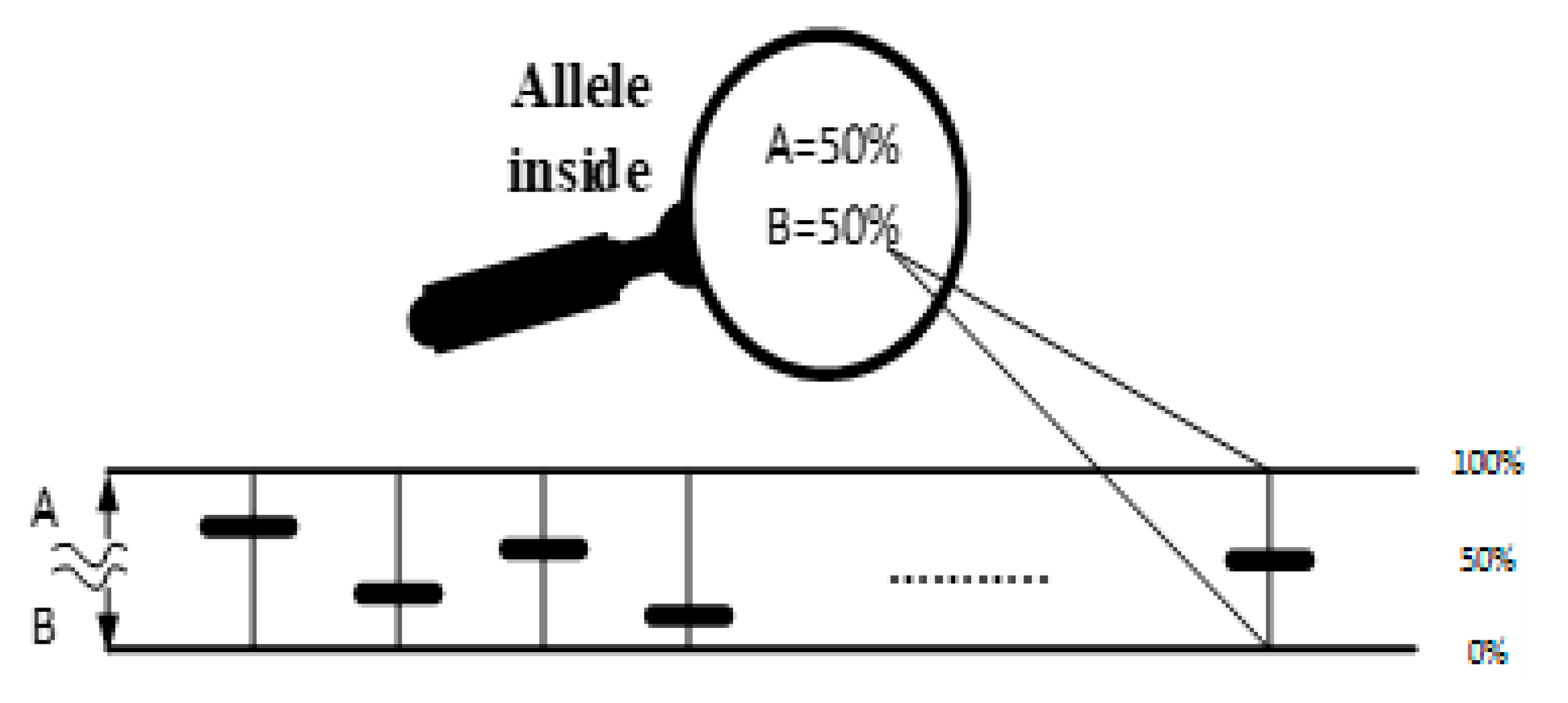
The structure of the proposed chromosome is presented in Figure 4, where each allele has represented by A and B.

These properties can be affected by mutation (

μ)

[28,29], positive mutation (

γ)

and negative (

δ

) mutations, where

γ

increases the positive attitude(A). Conversely, the negative attitude (B) will decrease according to Eq. (4) and vice versa. The following algorithm shows the mutation process affecting the allele (A&B). Suppose that the mutation (

μ)

comes randomly (positive or negative), as follows:

μ = \{\begin{matrix} γ + v e \\ δ, - v e \end{matrix}

(5)

γ = \{γ_{1}, γ_{2} \dots \dots ., γ_{n}\}

(6)

δ = \{δ_{1}, δ_{2} \dots \dots ., δ_{n}\}

(7)

The value(weight) for each mutation should be minimal about

\frac{μ}{1000}

, especially with numerical crossover. So, the change would be small with each crossover.

Step 1: Start

Step 2: Initialize each n population chromosomes randomly

Step 3: Generate random Mutation (

μ

)

Step 4: If

μ

γ

= +evA is increased and B decreased // Evaluation mutation

Step 5: Else If

μ

δ

= -ev
A is decreased and B increased

Step 6:

A_{i} + B_{i}

Step 7: End.

5. Oriented Crossover (OC)

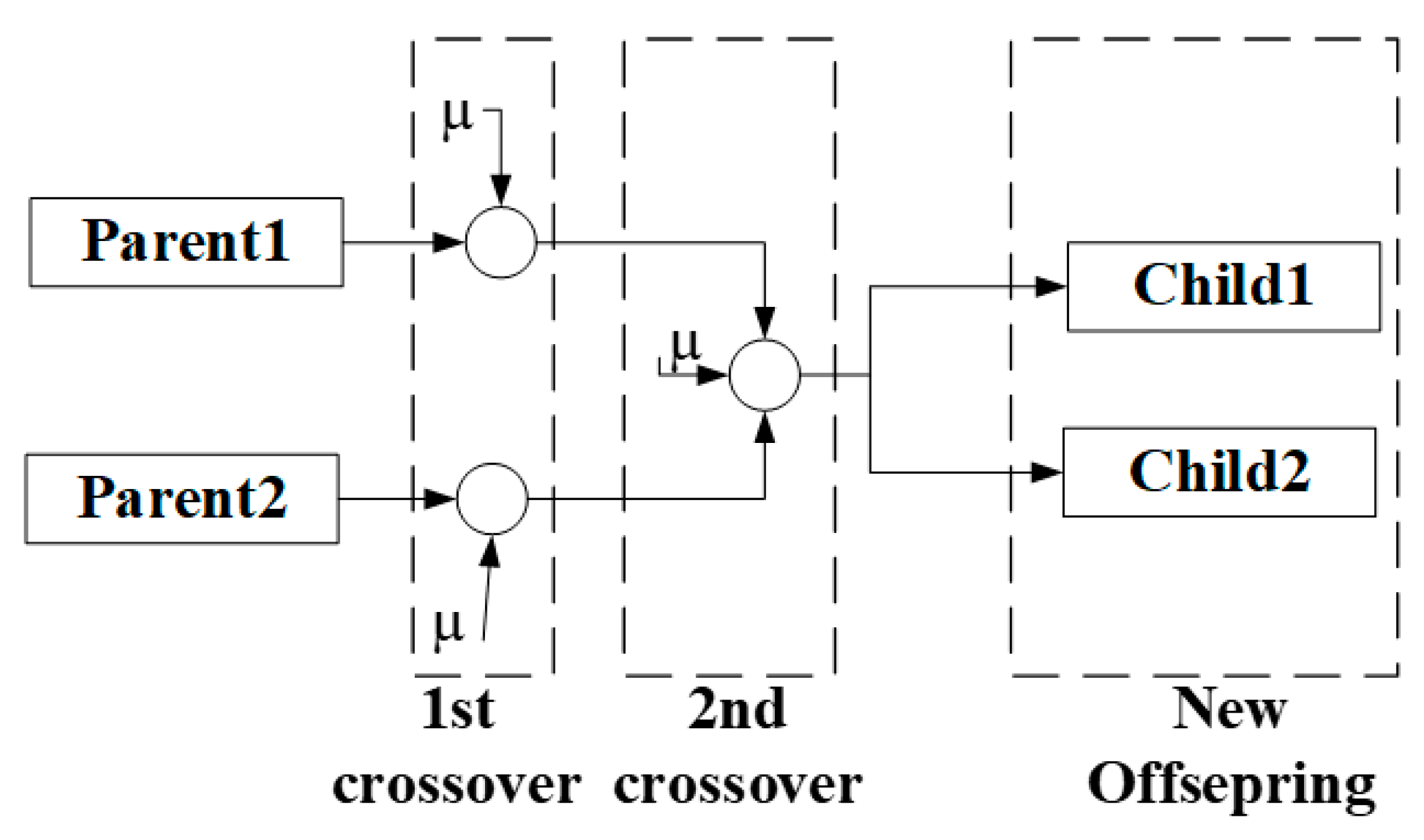
This system is supposed to enhance the allele by improving one attitude at the expense of the other by applying the mutation weight. As the first step, this crossover happens for the single parent, and the effect of µ would make a change for the alleles. If this crossover could not improve the system (or reach the target), the second crossover applies to mate the parent. Figure 6 shows the oriented crossover. The proposed crossover can apply to binary crossover and numerical crossover.

Figure 5. Oriented crossover.

5.1. First Crossover

5.1.1. Binary Crossover

We can represent this crossover for A and B attitudes to obtain a binary form for each gene by Eqs. (8) and (9).

A_{n n}^{P} = [\begin{matrix} A_{11}^{p} | γ_{11} \\ A_{22}^{p} | γ_{22} \\ \dots \\ \dots \\ A_{n n}^{p} | γ_{n n} \end{matrix}]

(8)

B_{n n}^{P} = [\begin{matrix} B_{11}^{p} | δ_{11} \\ B_{22}^{p} | δ_{22} \\ \dots \\ \dots \\ B_{n n}^{p} | δ_{n n} \end{matrix}]

(9)

After implementing Eq. (8) and Eq. (9), the new attitudes should be getting for the same single parent, then need to add logically (OR) both Attitudes to get a newly single parent, as in Eq. (10):

P_{n}^{S} = [\begin{matrix} A_{11}^{P} | B_{11}^{P} \\ A_{22}^{P} | B_{22}^{P} \\ \dots \\ A_{n n}^{P} | B_{n n}^{P} \end{matrix}]

(10)

where

μ = \{\begin{matrix} 1 \equiv δ \\ 0 \equiv γ \end{matrix}

, P: new parent, p: particular individual for the same parent.

5.1.2. Numerical Crossover

This type of crossover works with finite quantities for A, B, and µ. The weight of µ has three levels as Eq. (11).

{μ|}_{\forall_{γ, δ}} = \{\begin{matrix} H i g h \\ m e d i a m \\ l o w \end{matrix}

(11)

where µ chooses to be very small.

The crossover for numerical crossover obtained by two cases depending on the type of µ (+ve or –ve), whatever its weight:

In case of µ come in +ve state:

A_{n n}^{P} = [\begin{matrix} A_{11} (1 + γ_{1}) \\ A_{22} (1 + γ_{2}) \\ \dots \\ \dots \\ A_{n n} (1 + γ_{n}) \end{matrix}]

(12)

B_{n n}^{P} = [\begin{matrix} B_{11} (1 - γ_{1}) \\ B_{22} (1 - γ_{2}) \\ \dots \\ \dots \\ B_{n n} (1 - γ_{n}) \end{matrix}]

(13)

In the case of µ comes in the negative (-ve) state:

A_{n n}^{P} = [\begin{matrix} A_{11} - B_{11} \times δ_{1} \\ A_{22} - B_{22} \times δ_{2} \\ \dots \\ \dots \\ A_{n n} - B_{n n} \times δ_{n} \end{matrix}]

(14)

B_{n n}^{P} = [\begin{matrix} B_{11} (1 + δ_{1}) \\ B_{22} (1 + δ_{2}) \\ \dots \\ \dots \\ B_{n n} (1 + δ_{n}) \end{matrix}]

(15)

P_{n n}^{P} = [\begin{matrix} A_{11}^{n e w} + B_{11}^{n e w} \\ A_{22}^{n e w} + B_{22}^{n e w} \\ \dots \\ \dots \\ A_{n n}^{n e w} + B_{n n}^{n e w} \end{matrix}]

(16)

5.2. Second Crossover

We can call this type of crossover a mate crossover because this crossover between the parents comes after the first crossover. This crossover has been represented in Eq. (17) and Eq. (18).

P_{1 i}^{O F S} = μ_{i} P_{1 i}^{p} + (1 - μ_{i}) P_{2 i}^{p}

(17)

P_{2 i}^{O F S} = μ_{i} P_{2 i}^{p} + (1 - μ_{i}) P_{1 i}^{p}

(18)

where; each

P_{1 i}^{O F S}

and

P_{2 i}^{O F S}

refer to new offspring to the corresponding parent.

Second crossover is equivalent to uniform crossover [1].

6. Experimental Work

6.1. The Experimental Work Procedures

This section shows the empirical implementation of the proposed system. The proposed algorithms are used as an optimization method. Our procedures go with the procedure in the next section.

6.2. Optimization Implementation Procedures

Here we have shown the practical implementation of the proposed system. Our procedures go with the following algorithm.

Step 1: Initialization for population chromosomes starts by generating random individuals as initialization, each individual’s chromosome with ten “A” attitude alleles for each, as proposed in section 4.

Step 2: The boundary of A [0,1] for binary crossover, and from 0.1 to 0.9, each allele for the numerical crossover.

Step 3: Take the complements of A for each allele to generate B allele, as have been discussed in Section 4 of the article.

Step 4: Calculating the cost function for each parent depends on which equation needs to be optimized.

Step 5: Generate and test four isolated pupations for each equation in Eq. (8-11) and one for numerical crossover with Eq. (17).

6.3. General Optimization Test

Here we display two equations that have been used for general mathematical optimization:

Uneven Decreasing Maxima Function [2,30]: this is one of the multimodal optimization problems.

F = e^{(- 2 \log (2) {(\frac{\emptyset - 0.08}{0.854})}^{2})} {s i n}^{6} (5 π (\emptyset^{\frac{3}{4}} - 0.05))

(19)

where

\emptyset \in [0,1]

. The aim is to obtain an optimal value of

\emptyset

Himmelblau Function: this function, which is used by [2,31] ; it is defined as:

F = 200 - {(\emptyset_{1}^{2} + \emptyset_{2} - 11)}^{2} - {(\emptyset_{1} + \emptyset_{2}^{2} - 7)}^{2}

(20)

where

\emptyset_{i} \in [- 6,6]

. The aim is to obtain optimal values of

\emptyset_{1,} \emptyset_{2}

6.4. Communication and Network Optimization 6.5. Fractal-Based WSN Optimization

Step1: Optimize the parameters in computer networks as Eq. (21) and Eq. (22), which leads to minimize the value of F.

F = \sum_{i = 1}^{n} x_{i} y_{i}

(21)

F = \sum_{i = 1}^{n} {(x_{i} y_{i})}^{2}

(22)

Step2: Choose ten individuals to represent the first generation, then calculate the fitness of this generation or Generation Fitness (

G_{T})

as Eq. (23).

G_{T} = \sum_{i = 1}^{n} C_{i}^{p}

(23)

where; n: number of individuals in that generation,

C_{i}^{p}

, referring to the individual p cost function, the fitness is calculated by applying Eq. (19 - 23), then calculating the fitness of each individual as Eq. (24).

f_{i}^{p} = \frac{C_{i}^{p}}{G_{T}}

(24)

Step3: Calculate the probability for each individual as Eq. (25)

{P r o b}_{i} = f_{i}^{p} * n

(25)

Then rearranging the individual depends on the probability of choosing the best individual to be a good selected parent in this generation.

Step4: After arranging the individuals in decreasing order, eliminate the last two individuals (the two least probability).

Step5: After eliminating two individuals, it now has the best parents ready to mate; thus, it makes the crossover according to the proposed OC algorithm to get new offspring as a new generation.

Step6: Repeat the steps from (2) to (6) again till they reach only two individuals in the offspring.

Step7: Repeat steps (1) to (7) for one hundred iterations to choose optimal values.

Step8: The steps from (1) to (8) are implemented with Eq. (19-22).

In this section, the proposed method applying with fractal-based design for wireless sensor network (WSN) nodes for optimization. This method depends on Fractal design where the fractal is geometrically based patterns and structures that can repeat in any size, from the largest shape to the symmetric smallest shape. Sierpinski triangle [32,33] well known fractal model. Figure 6 shows the WSN nodes based Sierpinski triangle.

From Figure 6, supposed that the nodes deployed as Sierpinski triangle fractal, for static task(message) scheduling. The purpose of optimization to reduce the overhead on the nodes. The overhead increasing when the message delivered to the base of the triangle. Sierpinski triangle nodes topology construct under two formulas:

General formula for nodes numbers is:

N = 3 * 2^{k}

(26)

where,

N

is the number of nodes, and

k = 0, 1, 2, \dots, m

General formula for number of links (edges) is:

L = (N * d) / 2

(21)

wheredis the degree of node.

Eq. (27) will be used in Section 7.6 of this article.

6.6. Recursive Process

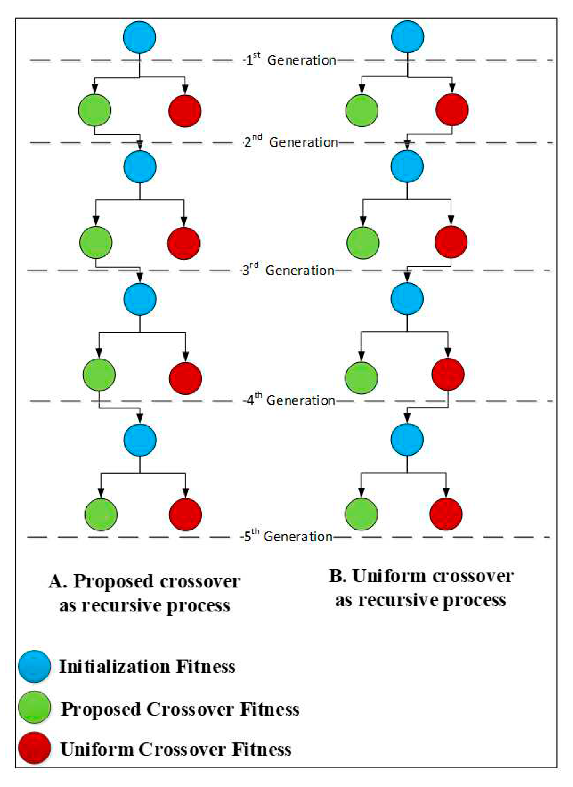
The experimental work is done by numerous recursive processes, which implies that each generation's output will serve as the next generation's input. However, it will depend on which crossover will act as the next generation's input. The recursive process for generations depends on their finesses. Figure 7 shows the flow work of the recursive processes.

In this article, the experimental work was tested for five generations. In Figure 7 the symbols mean the initialization refers to the parent selection process for the parents; after selection. The blue ball refers to the initialization fitness values which tested all types of crossover methods. The output will consist of two balls, red and green, where red represents the output from the implementation of uniform crossover (UC) methods and green represents the output from the implementation of OC crossover methods.

Figure 7-A shows the OC fitness as a recursive fitness input for the next generation. Figure 7-B shows the UC fitness as a recursive fitness input for the next generation. The benefits of using different recursive methods, are to show the influence of the proposed method even applying the shortcoming output from UC. The proposed method shows its outperforming in two methods. The steps in sub-sections 6.2, 6.3, and 6.4 have been implemented for UC and OC crossover with each generation.

6.7. Implementation Phases

This article implemented the experimental work as two phases for high performance and they are as follows:

Phase one: this phase implements the proposed work for optimization related the differential equations and network optimization with comparing with one type of crossover, is UC, this is because it closed characteristics to the proposed work.
Phase two: in this phase implements the proposed work as mentioned in phase one for optimization with comparing the evaluation with UC, NC (with different values of N), and QC [19].

7. Results and Discussion

7.1. Genetic Algorithm Parameters

We have carried out various experiments and their implementations in MATLAB programming (under Academic License 40635944). Some of the function parameters bounders we could not commit with it because they may not apply with a binary crossover on which we depend and propose according. Table 1 shows that the GA parameter has been dependent on this work. The results of article compare with a uniform crossover because it is closest to the proposed work, and compared with other crossovers, got meaning less even the proposed work outperformed. The empirical results perform in two ways, generations fitness calculation comparison and equilibrium generations fitness over one hundred iterations.

7.2. Binary Crossover under Phase One

Here we discuss about the binary crossover evaluation for chromosome contents. The cost function for each individual has been calculated after converting the binary to decimal values. The binary crossover was implemented for five generations to test the four Eq (19-22).

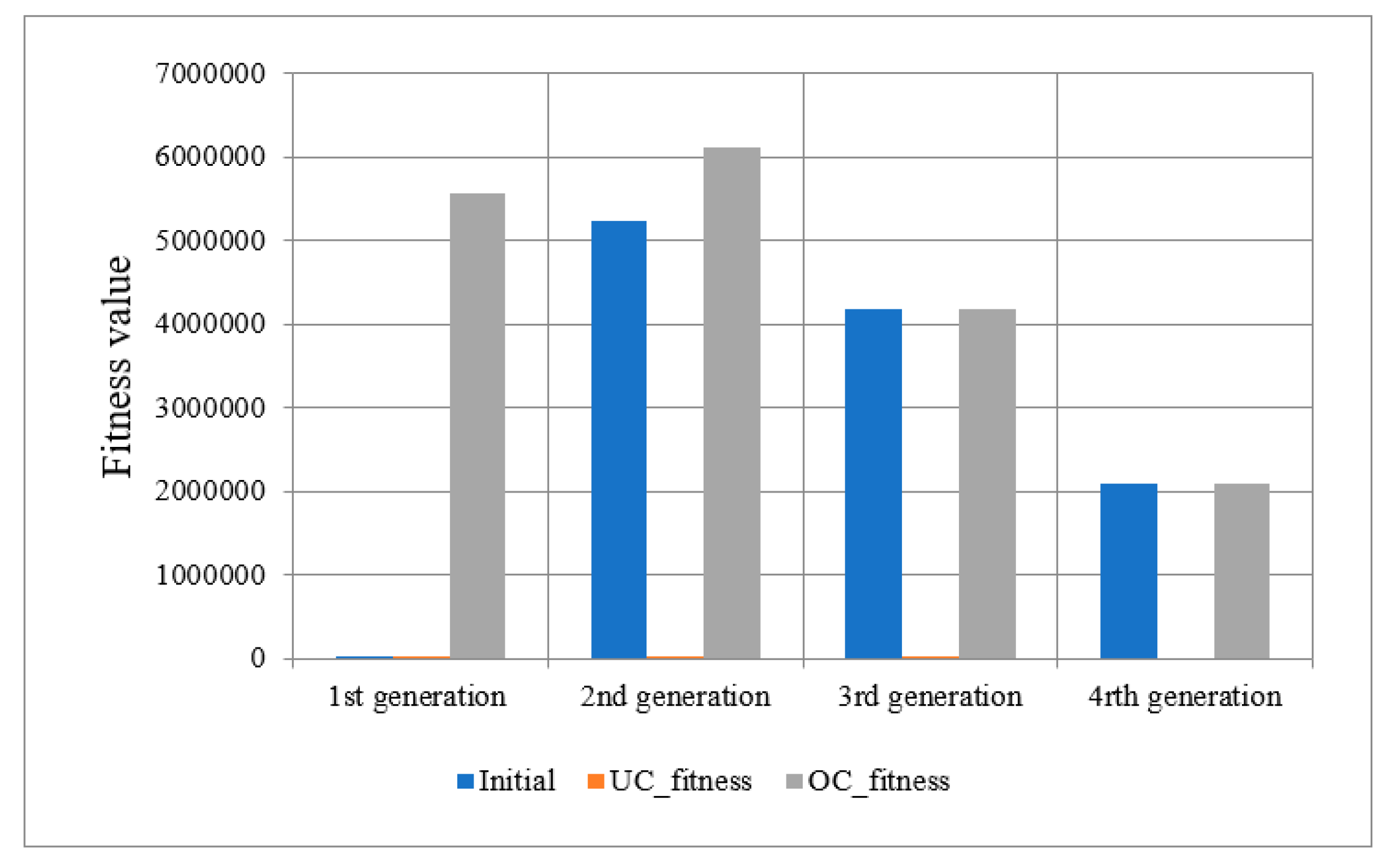
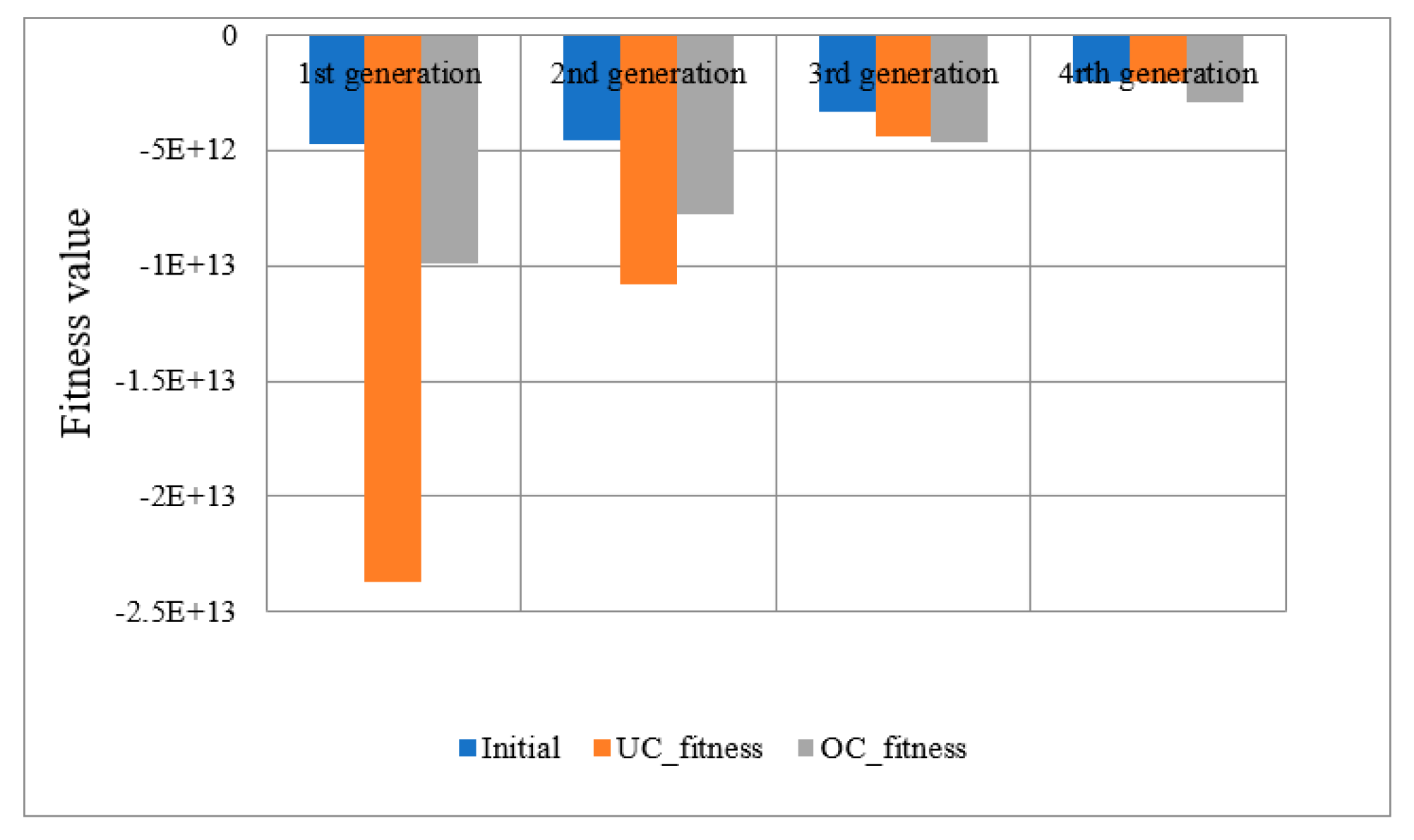
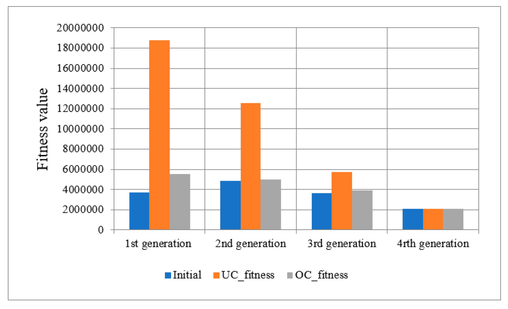
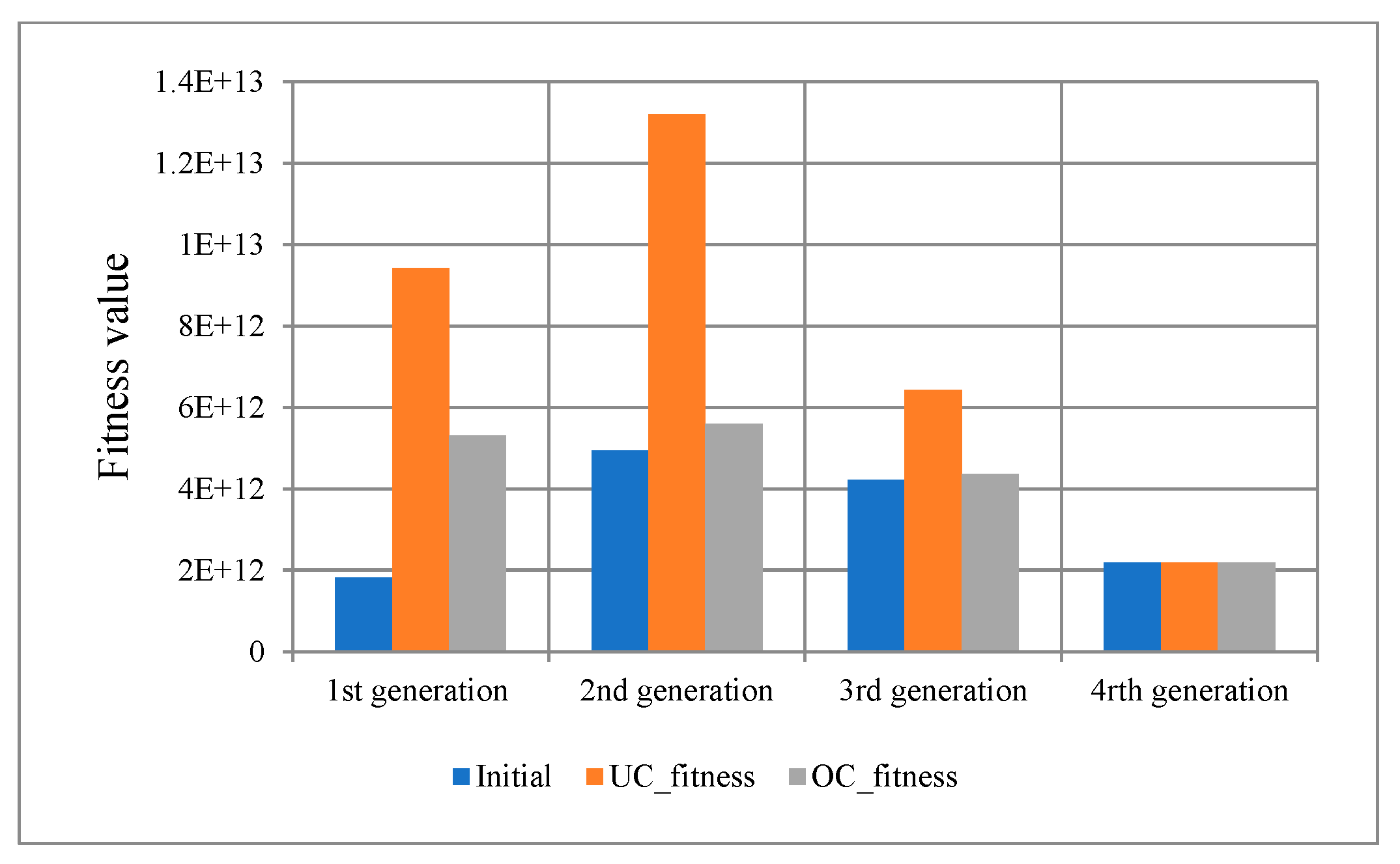
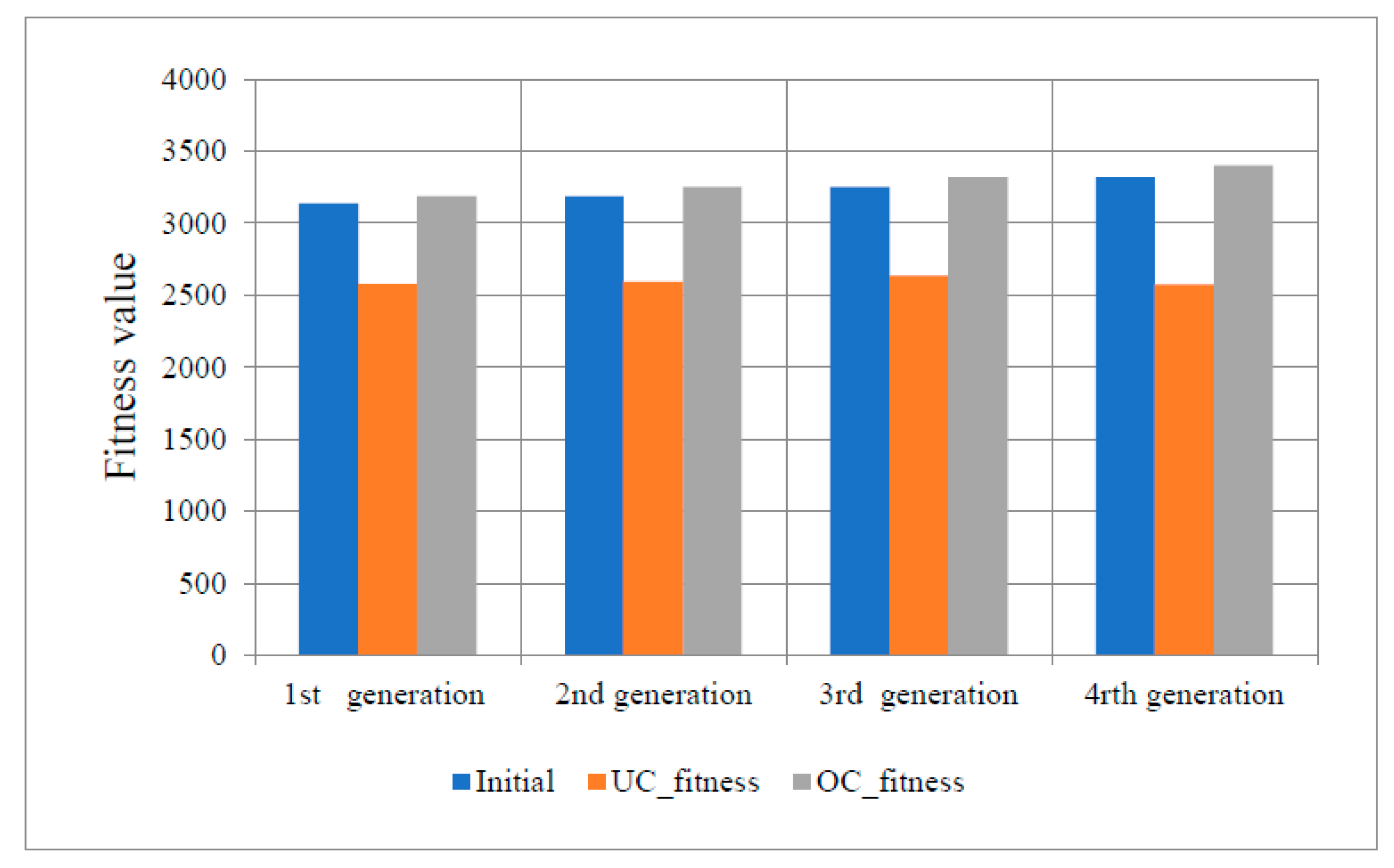
The comparison between all algorithms depends on the population's fitness for each generation. The experimental evaluation did for both; the proposed system and standard uniform crossover. The fitness comparisons are shown in Figure 8, Figure 9, Figure 10 and Figure 11. They are show the comparison between the original population fitness without applying any algorithm; we called it “Initial”, and this population needed to optimize, whereas, few researchers have applied UC, and OC. Figure 8 shows implemented Eq. (19); from the figure we can see that

OC is working as required better than UC. Figure 9 shows the implementation for Eq. (20); note that OC was retrieved in the last generation. For Figure 10 and Figure 11, the OC worked well, with little outperforming for UC.

7.3. Numerical Crossover under Phase One

With Numerical crossover used, in this article, the floating points representing A or B attitudes are used randomly (range from 0.1 to 0.9). For this type of crossover, the following equation is used for the cost function:

F = \sum_{i = 0}^{n} z^{i}

(22)

where z refers to the parameters related to Eq. (1) to calculate the fitness for each link i. Thus; it’s the application of communication and networking.

The implementation was done for Initial, UC, and OC finesses. Figure 12 shows the fitness optimization comparison, where the OC shows the outperform.

7.4. Equilibrium State under Phase One

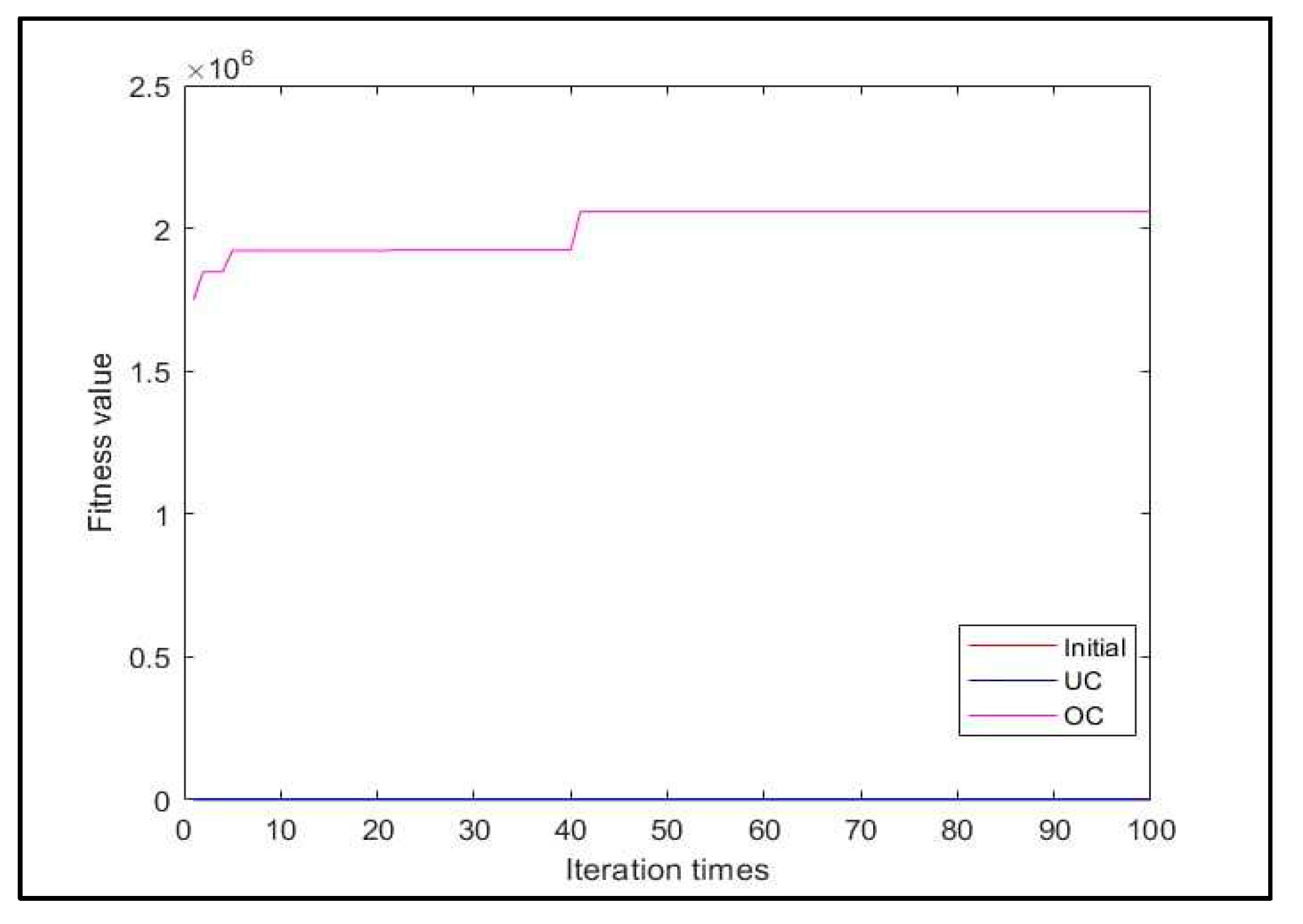
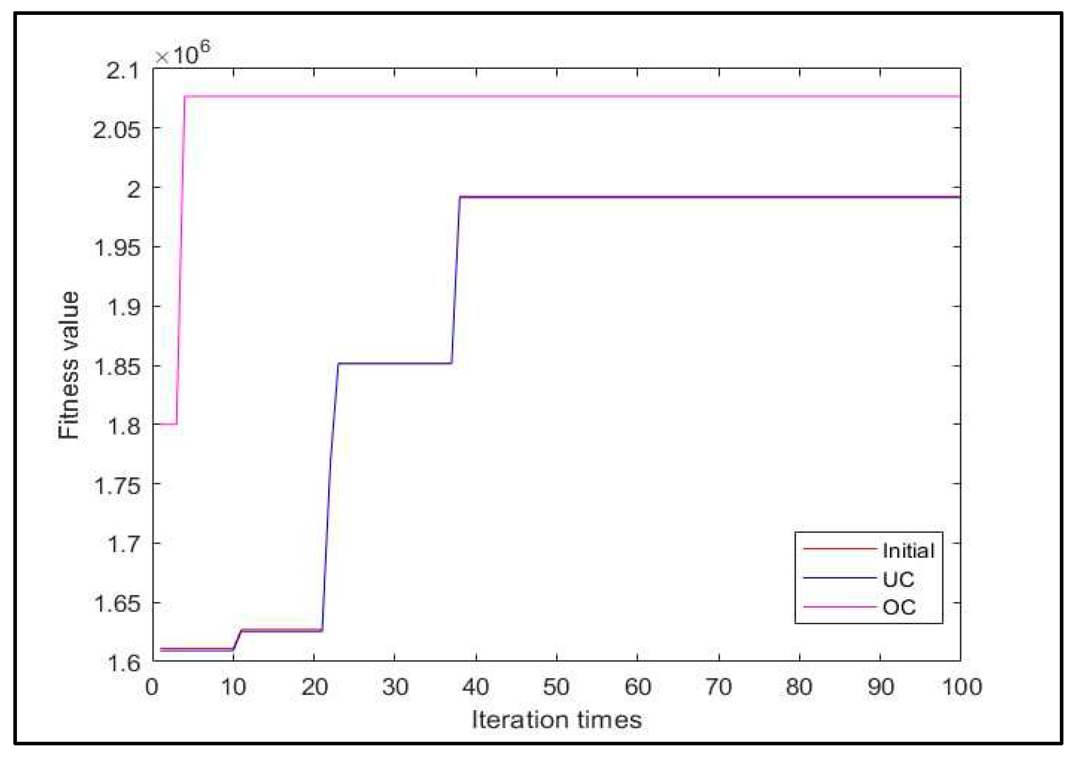
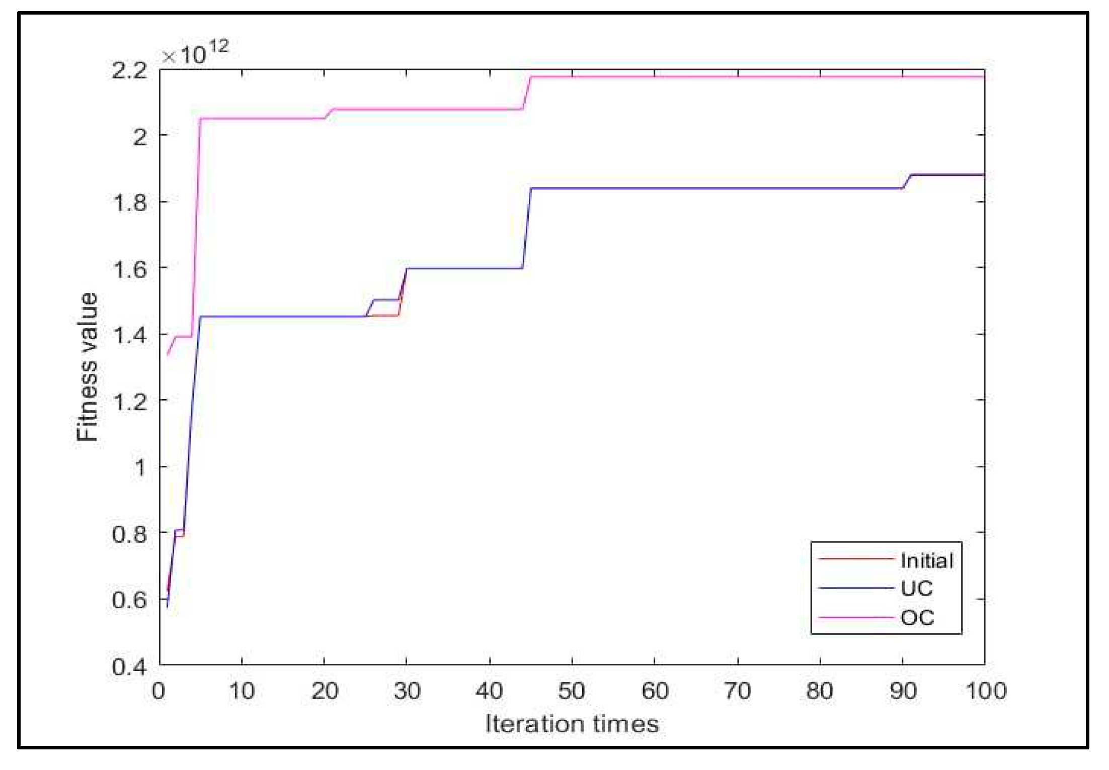
This section shows the searching experiments for the best optimization after one hundred iterations, with four generations from the selected population for every iteration. Figure 13 shows the times of iterations to reach the equilibrium state for Eq. (19). Figure 14 shows the equilibrium state for equation (21). The implementation for Eq. (22) showed in Figure 15 For Eq. (20), the equilibrium state for all algorithms has the same characteristics in the chart.

7.5. Binary Crossover under Phase Two

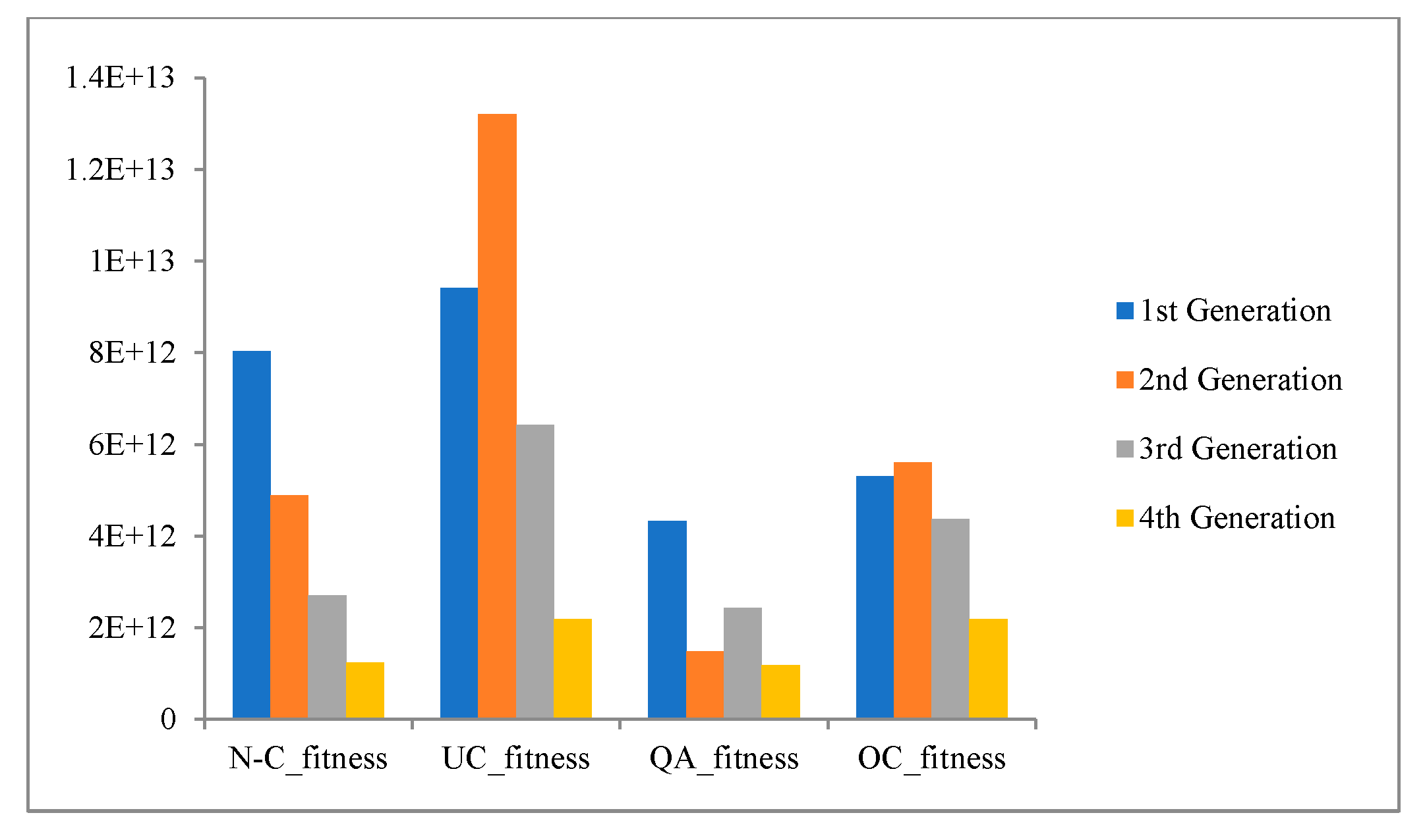
In this discussion, the assessment of chromosome contents using binary crossover has been explored. The cost function for each individual is determined by converting the binary values to decimal. The binary crossover technique is tested for four equations (19-22) over four generations. The performance of different algorithms is compared based on the fitness of the population for each generation. An experimental evaluation is conducted on the proposed system (OC), UC, NC , and QC. 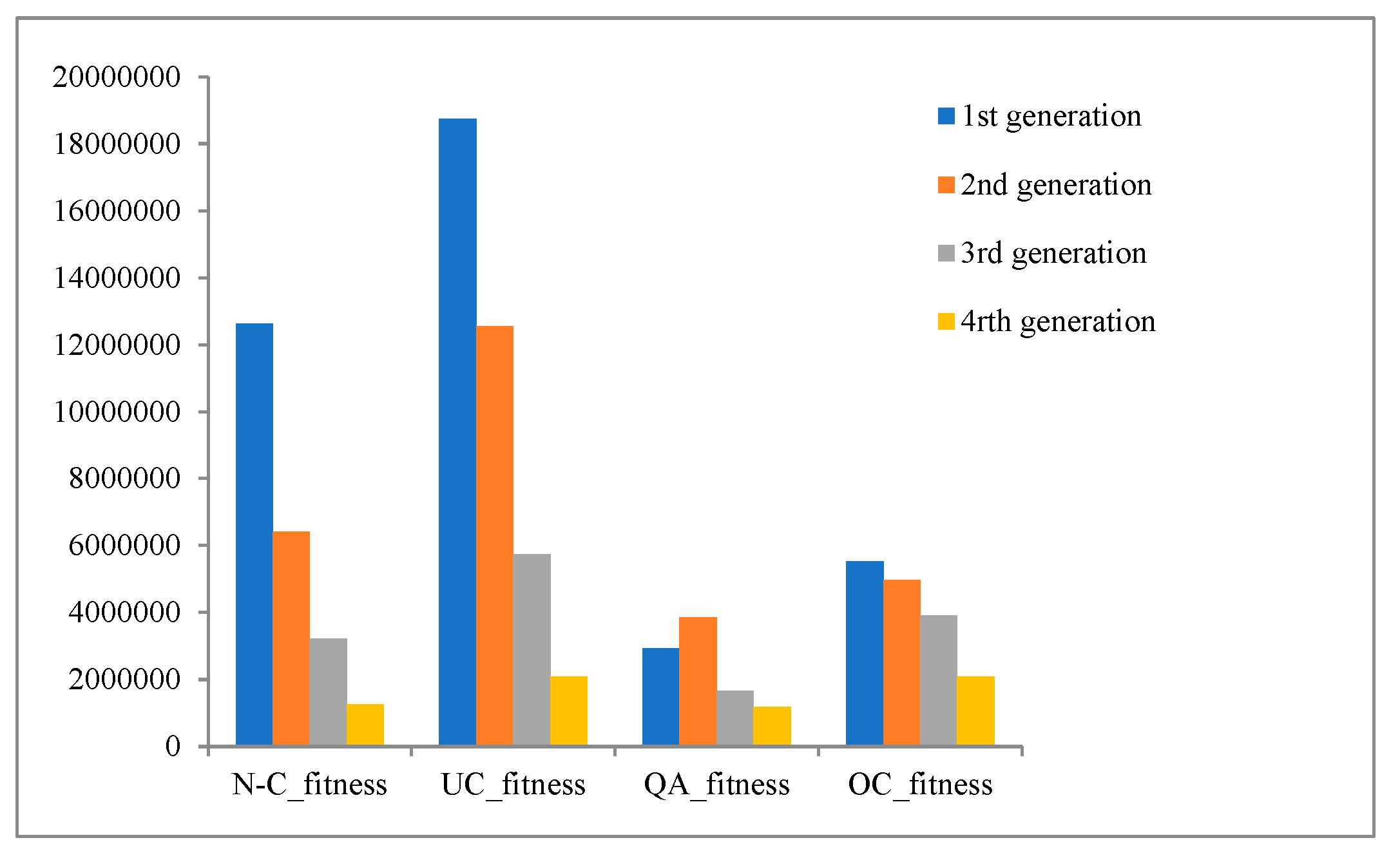The fitness comparisons are illustrated in Figure 16, Figure 17, Figure 18 and Figure 19, which depict the comparison between the initial population fitness and populations that have undergone optimization using UC, NC, QC and OC. 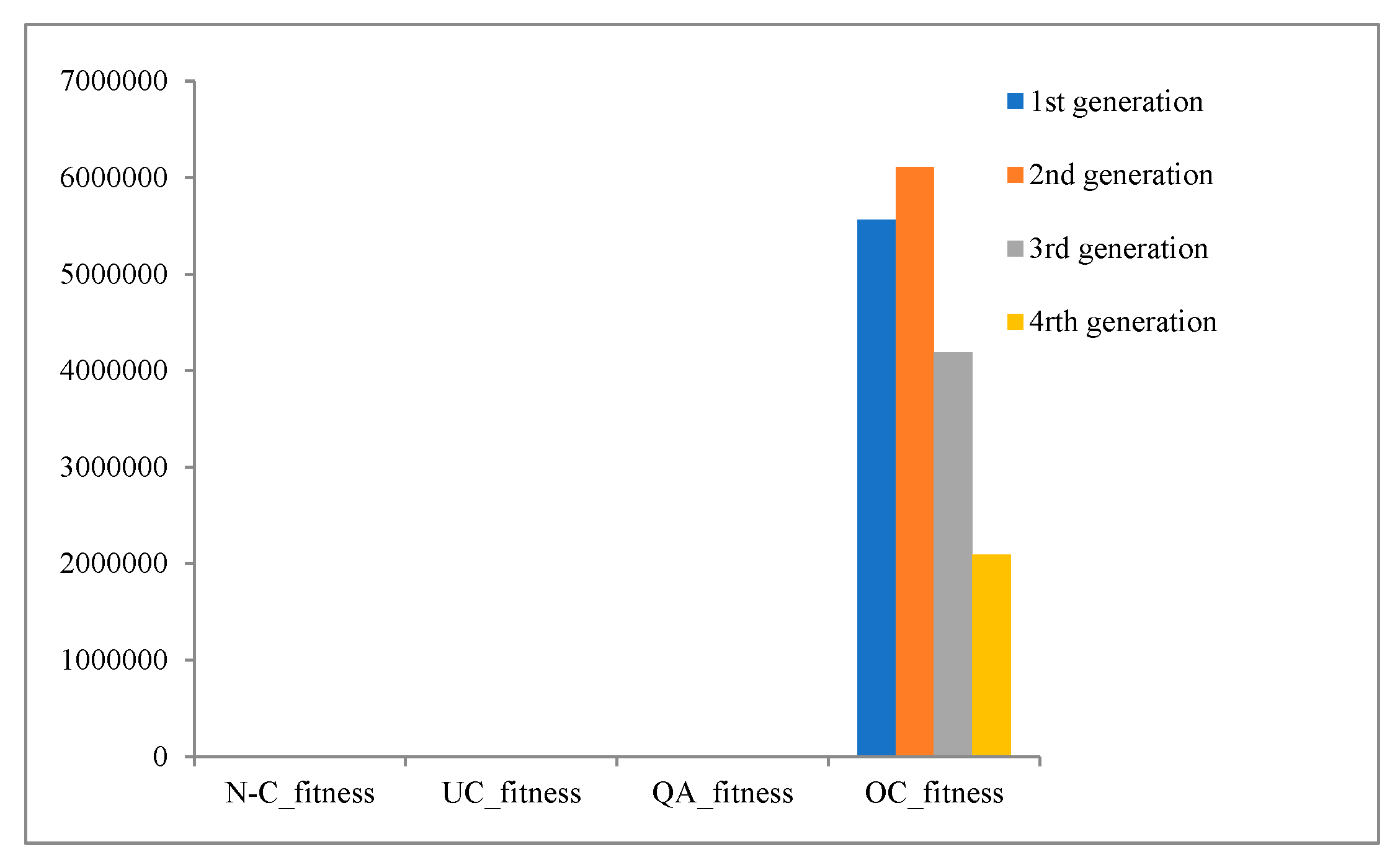Figure 16 shows the implementation of Eq. (19), and it is evident that OC performs has been gradually minimized the fitness’s across the generations better than the others. 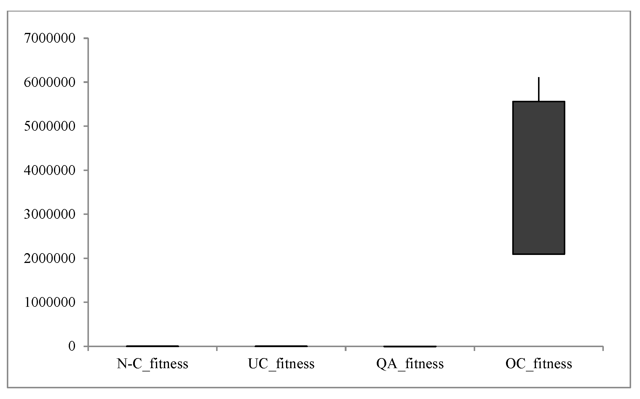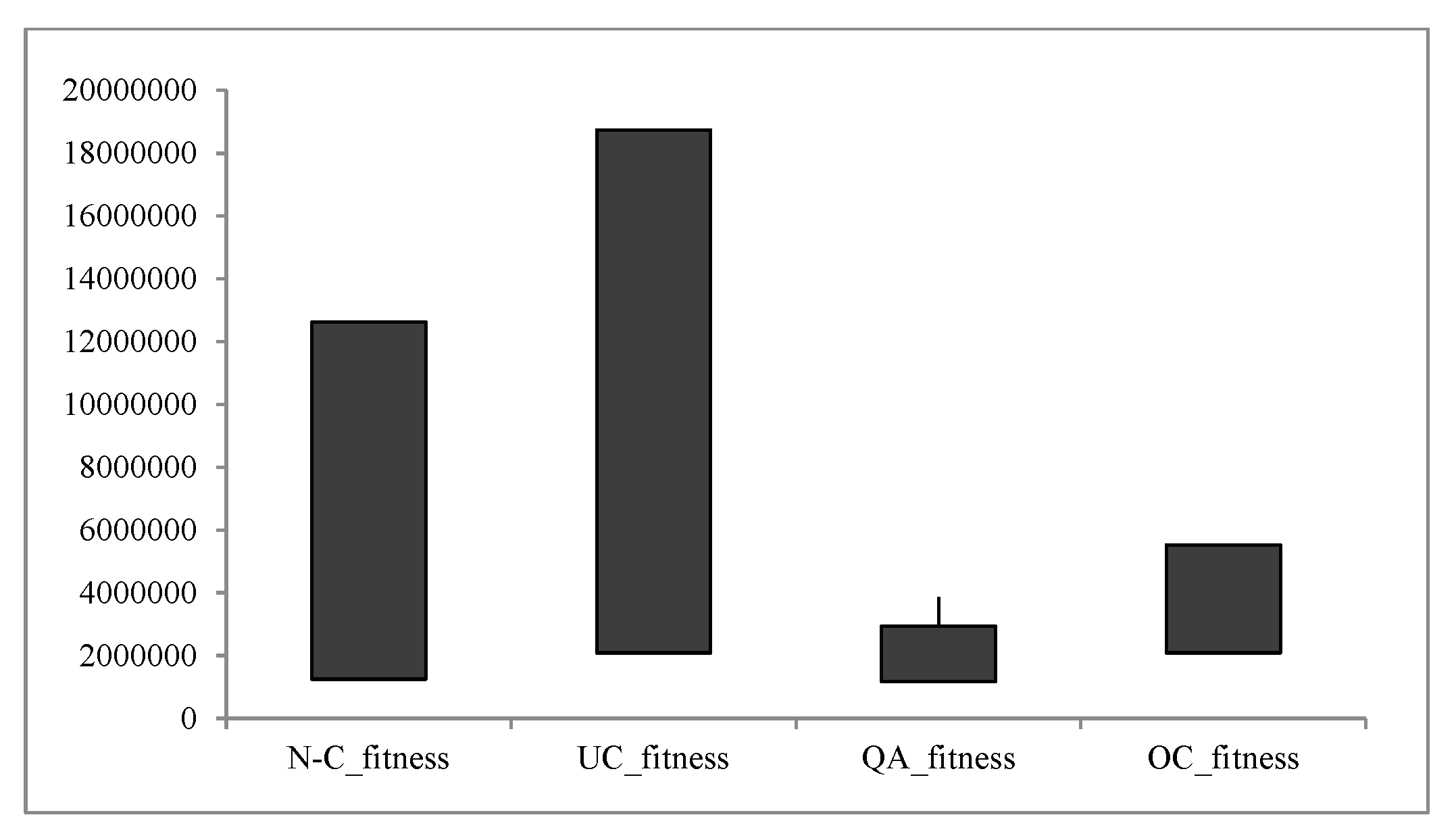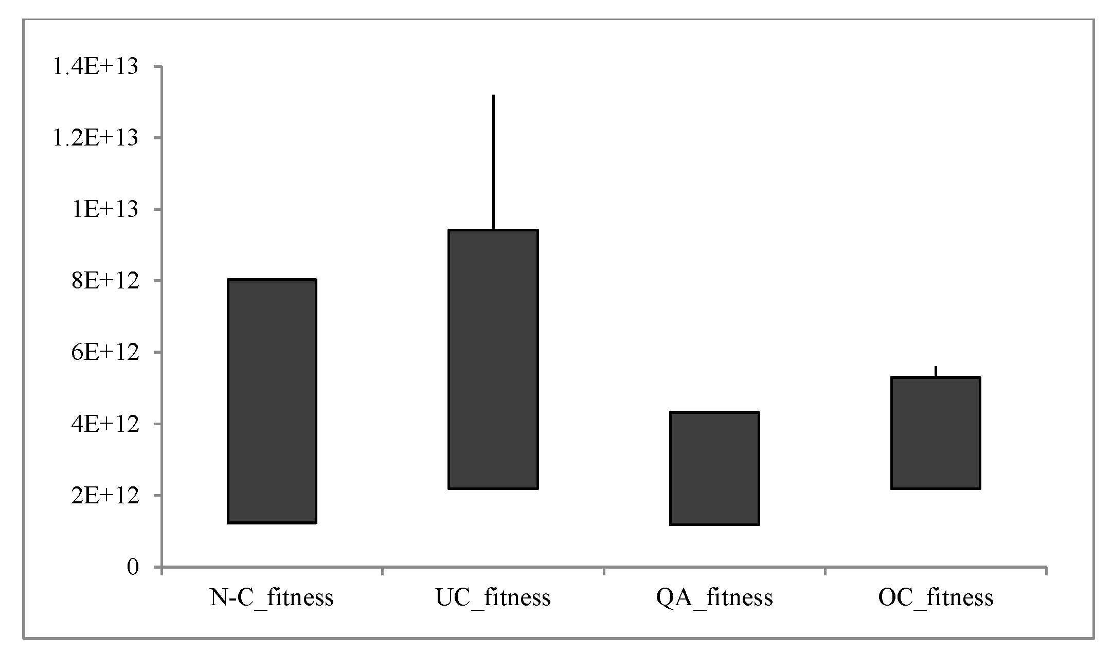Figure 17 show the representation of the fineness by Japan’s candles to show retrieved the other fitness compared to OC. Figure 18 demonstrates the implementation of Eq. (20), although the QC was approached to the maximum optimization first, but the maximization seems not suitable for all systems, because it suitable for specific and low range (from min. to max.) optimization, and such behavior does not suitable in the many applications. Elsewhere the OC was gradually maximized and it is was better than the other and seem to be suitable with different systems. Figure 19 shows clearly that OC has a gradually optimization and good performance with standard crossovers, in contract of QC lock like a special case optimization in this system.

7.6. Numerical Crossover Phase Two

The evaluation of this section to represented the network and fractal WSN optimization. Then Comparing the performance for OC and the other types of crossover’s fitness.

As mentioned in section 7.3, numerical crossover is employed, and the floating points randomly chosen to represent A or B attitudes. The values used ranged from 0.1 to 0.9. The parameters used in this section for optimization depend on N, and L from Eq. (27 & 28) respectively, to substitute in Eq. (20 & 21). The optimization for these equations used for minimization.

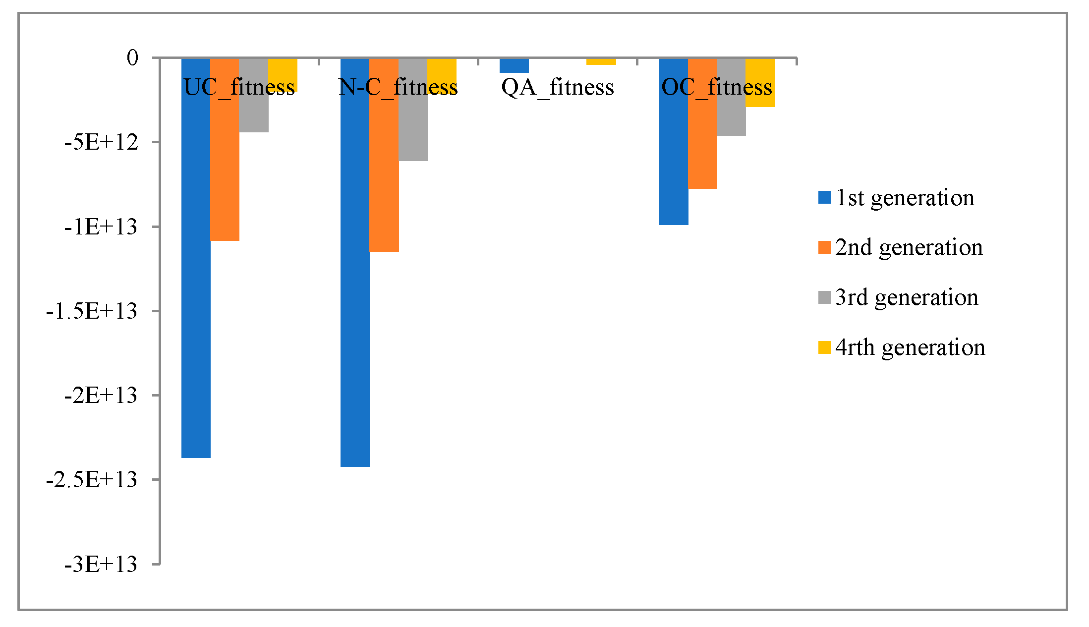
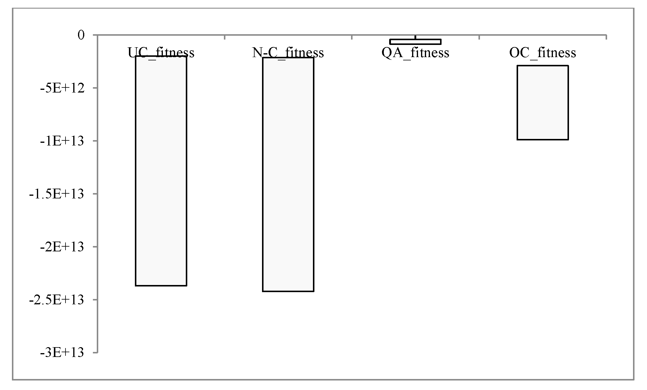
Figure 20 and Figure 21 show the fitness optimization comparison and implementation using Eq. (20), the figures shows that OC performance is gradually did the minimization, and clearly outperform UC, but comparing with the NC is retrieved, but the OC practically more suitable because it depends on fractal geometric shape, and this need gradually optimization through generations (in case representing each level of node to be equivalent to each generation) to prevent the communication overhead. From other side QC gave better performance from OC only in the last generation. That is mean QC could give maximization in any level of generations, and this behavior does not suitable in network and communications.

Figure 22 and Figure 23 shows the fitness optimization comparison and implementation using Eq. (21), the figures indicates that the OC's performance decreased gradually and significantly outperformed the UC. However, the NC's performance is better than the OC's, but the OC is more practical due to its reliance on fractal geometry, which requires gradual optimization over multiple generations (if each node level is equivalent to a generation) to avoid communication overhead. On the other hand, the QC only outperformed the OC in the final generation, indicating that it could maximize performance at any generation, but this behavior is not suitable for networks and communications.

7.7. Equilibrium State Phase Two

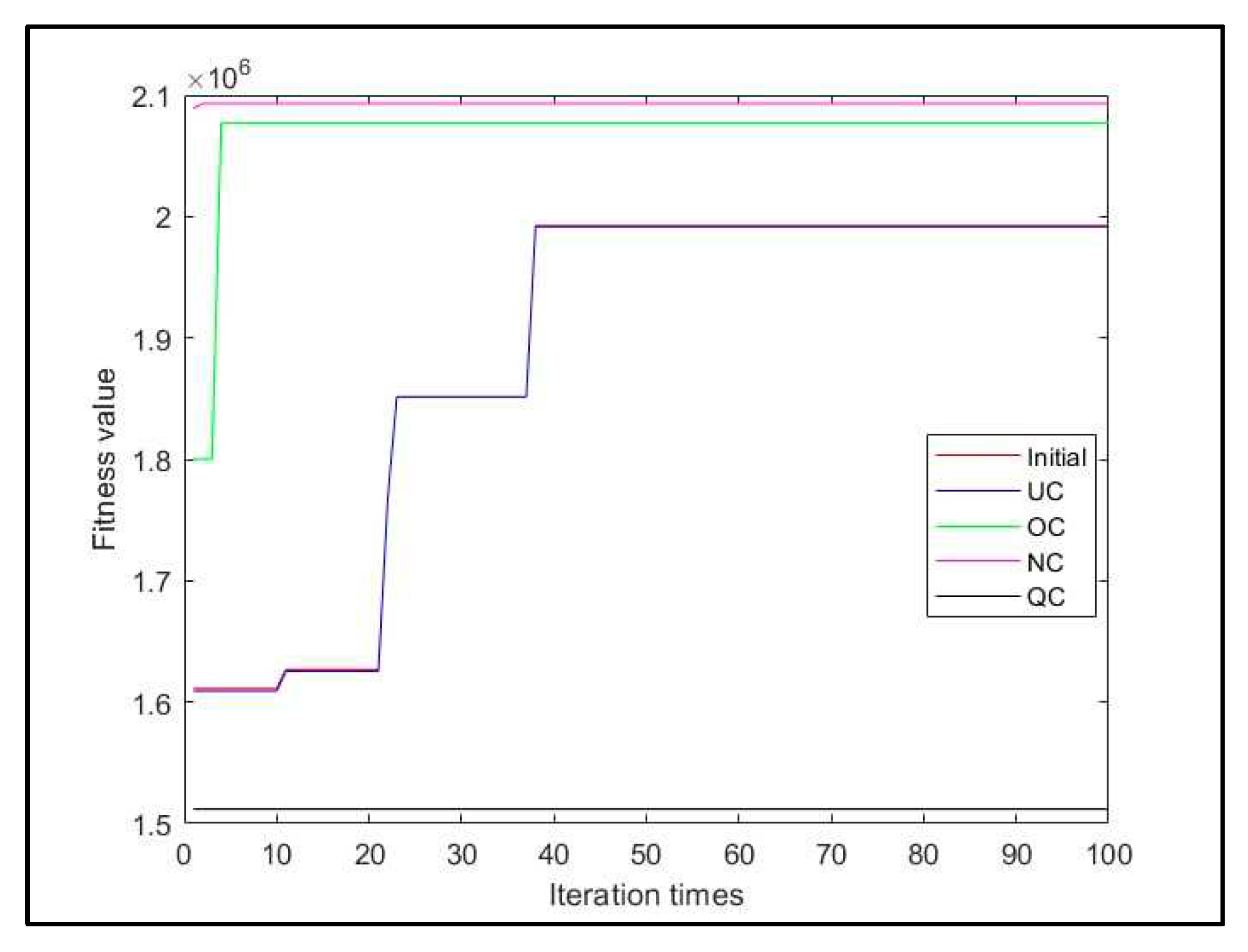
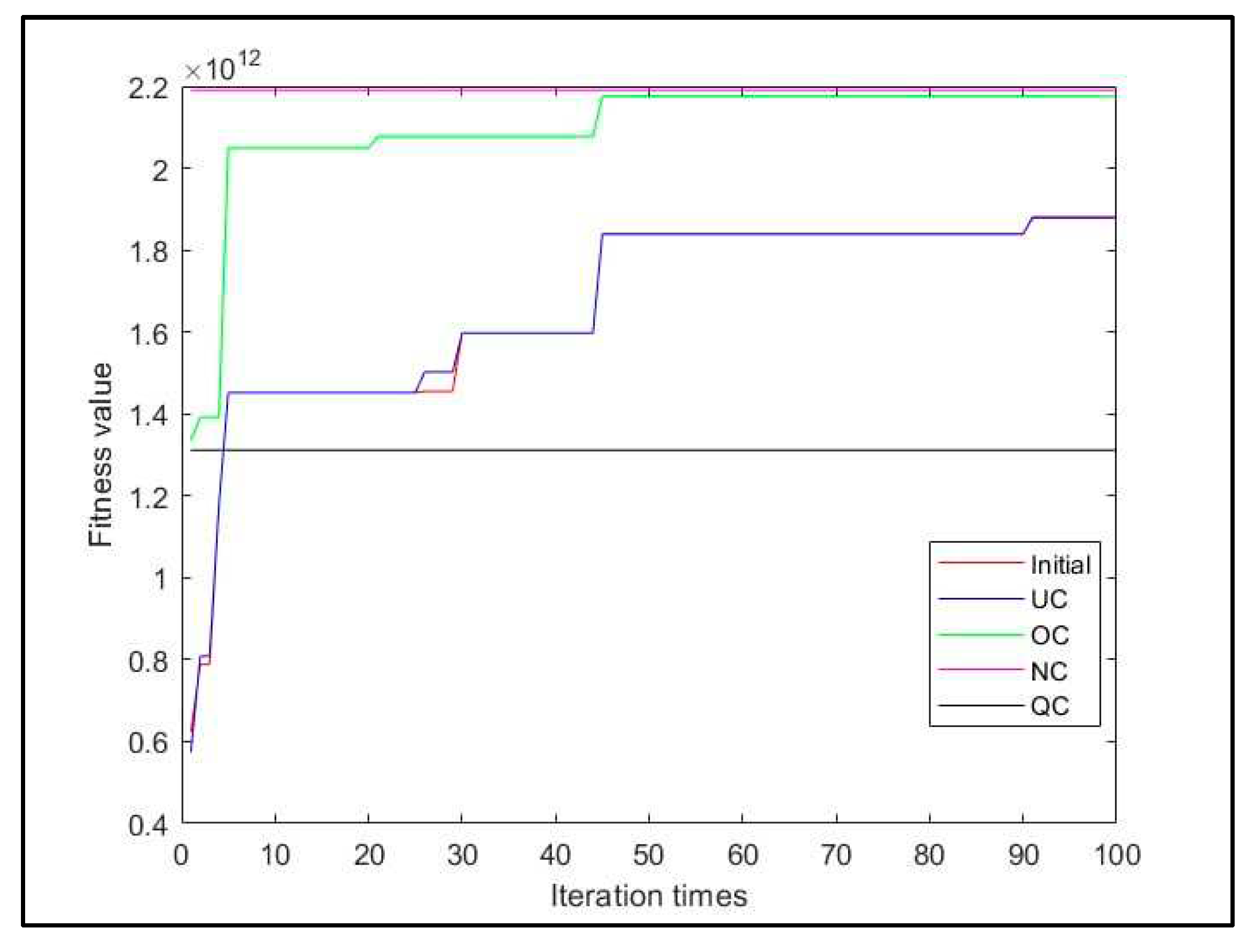
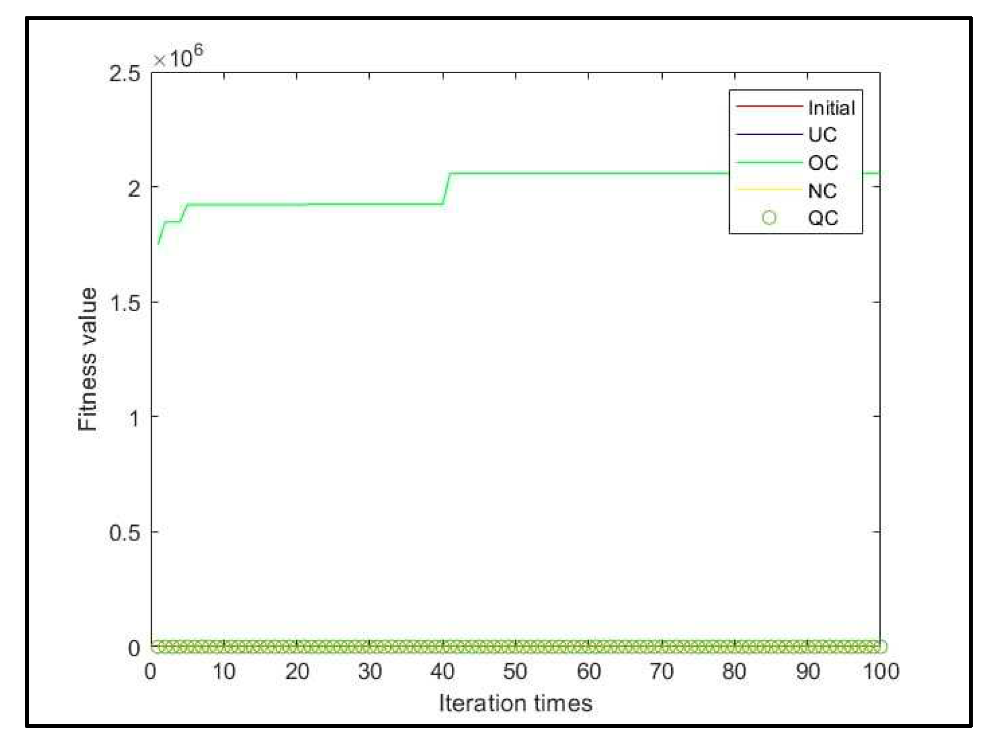
This section shows the searching experiments for the best optimization after one hundred iterations to the four types of crossover, with four generations from the selected population for every iteration. Figure 24 shows the times of iterations to reach the equilibrium state for Eq. (19). Figure 25 shows the equilibrium state for equation (21). The implementation for Eq. (22) showed in Figure 26. Figure 24 shows that the OC reaches to the constant state after 40 iterations but the other have no clear behavior. Figure 25 shows that OC reaches to the equilibrium stat after 5 iterations, better than UC, but there is no clear behavior in the others. In Figure 26, the QC looks like the intimal state, but OC has normal behavior and reached to constant state after 40 iterations.

8. Concluding Remarks

From the evaluation of the proposed method, we conclude that the application of the idea of using two properties (or attitude) in the allele, then performing such architecture to optimize in any system, indicated that computer networks, routing algorithms, and others will be more stable, especially when one of them is increased and the other decreased.

The proposed system is more suitable for numerical crossover from the experimental work because noted the OC outperforms the UC, NC, and many cased QC. The proposed work is instrumental in optimization for numerical calculations. In addition, the experiments proved that (OC) is very convenient for the purpose of optimization instead of (UC) Contribution.

The proposed work presents a new optimization method for Genetic Algorithms, which could improve the performance, especially if the system needs to improve the preferred parameters at the price of the unpreferred parameters.

The proposed optimization strategy would be useful in many disciplines, particularly in network and routing techniques.

9. Conflict of Interest

The authors declare no conflict of interest.

References

Kora, P. and P. Yadlapalli, Crossover operators in genetic algorithms: A review. International Journal of Computer Applications, 2017. 162(10). [CrossRef]
Abid Hussain, Y.S.M., Muhammad Nauman Sajid, An Efficient Genetic Algorithm for Numerical Function Optimization with Two New Crossover Operators. International Journal of Mathematical Sciences and Computing, 2018. 4(4): p. 1-17.
Mitchell, M., An introduction to genetic algorithms. 1998: MIT press.
Chiroma, H., et al., Neural networks optimization through genetic algorithm searches: a review. Appl. Math. Inf. Sci, 2017. 11(6): p. 1543-1564. [CrossRef]
Manzoni, L., L. Mariot, and E. Tuba, Balanced crossover operators in genetic algorithms. Swarm and Evolutionary Computation, 2020. 54: p. 100646. [CrossRef]
Holland John, H., Adaptation in natural and artificial systems. Ann Arbor: University of Michigan Press, 1975.
Spears William, Adapting Crossover in a Genetic Algorithm.
Gilbert Syswerda, Uniform Crossover in Genetic Algorithms. Proceedings of the 3rd International Conference on Genetic Algorithms, 1989.
Umbarkar, A.J. and P.D. Sheth, Crossover operators in genetic algorithms: a review. ICTACT journal on soft computing, 2015. 6(1). [CrossRef]
Sivanandam, S. and S. Deepa, Genetic algorithms, in Introduction to genetic algorithms. 2008, Springer. p. 15-37. [CrossRef]
Kirchner-Bossi, N. and F. Porté-Agel, Realistic wind farm layout optimization through genetic algorithms using a Gaussian wake model. Energies, 2018. 11(12): p. 3268.
Félix Patrón, R.S. and R.M. Botez. Flight trajectory optimization through genetic algorithms coupling vertical and lateral profiles. in ASME International Mechanical Engineering Congress and Exposition. 2014. American Society of Mechanical Engineers.
Bani-Hani, D., et al. Classification of leucocytes using convolutional neural network optimized through genetic algorithm. in Proc. of the 7th Annual World Conference of the Society for Industrial and Systems Engineering. 2018.
Zeidabadi, F.A. and M. Dehghani, Poa: Puzzle optimization algorithm. Int. J. Intell. Eng. Syst, 2022. 15: p. 273-281.
Anju, K. and K. Avanish, An advanced approach to the employee recruitment process through genetic algorithm. International Journal of Information Technology, 2021. 13(1): p. 313-319. [CrossRef]
Begum, S. and S.S. Padmannavar, Genetically Optimized Ensemble Classifiers for Multiclass Student Performance Prediction.
Haldulakar, R. and J. Agrawal, Optimization of association rule mining through genetic algorithm. International Journal on Computer Science and Engineering (IJCSE), 2011. 3(3): p. 1252-1259.
Muthana, S.A. and K.R. Ku-Mahamud, Comparison of Multi-objective Optimization Methods for Generator Maintenance Scheduling. methods (multi-objective metaheuristics). 14: p. 15.
F. Rabee, I. Jazaery and K. Kumar "Quaternary-Child Crossover for Genetic Algorithm in Real-Time Scheduling Optimization". International Journal of Intelligent Engineering and Systems, Vol 16, 2023.
Singh, N. and P. Chaurasia, A Review on Genetic Algorithm Operations and Application in Telecommunication Routing. 2019. [CrossRef]
Singh, J., An Optimal Resource Provisioning Scheme Using QoS in Cloud Computing Based Upon the Dynamic Clustering and Self-Adaptive Hybrid Optimization Algorithm.
Sanapala, R.K. and S.R. Duggirala, An Optimized Energy Efficient Routing for Wireless Sensor Network using Improved Spider Monkey Optimization Algorithm. transportation, 2022. 8: p. 9.
Jubair, A.M., et al., Optimization of Clustering in Wireless Sensor Networks: Techniques and Protocols. Applied Sciences, 2021. 11(23): p. 11448. [CrossRef]
Rangappa, M.H. and G.C. Dyamanna, Energy-Efficient Routing Protocol for Hybrid Wireless Sensor Networks Using Falcon Optimization Algorithm.
Cinat, P., G. Gnecco, and M. Paggi, Multi-scale surface roughness optimization through genetic algorithms. Frontiers in Mechanical Engineering, 2020. 6: p. 29. [CrossRef]
Forouzan, B.A., TCP/IP protocol suite. Fourth ed. 2010: McGraw-Hill Higher Education.
Changhyun Kwon, Julia Programming for Operations Research 2022(Second Edition). [CrossRef]
Schärfe, C.P.I., et al., Genetic variation in human drug-related genes. Genome medicine, 2017. 9(1): p. 1-15.
King, E.A., J.W. Davis, and J.F. Degner, Are drug targets with genetic support twice as likely to be approved? Revised estimates of the impact of genetic support for drug mechanisms on the probability of drug approval. PLoS genetics, 2019. 15(12): p. e1008489. [CrossRef]
Ortiz-Boyer, D., C. Hervás-Martínez, and N. Garcia-Pedrajas, Cixl2: A crossover operator for evolutionary algorithms based on population features. Journal of Artificial Intelligence Research, 2005. 24: p. 1-48.
Li, X., A. Engelbrecht, and M.G. Epitropakis, Benchmark functions for CEC’2013 special session and competition on niching methods for multimodal function optimization. RMIT University, Evolutionary Computation and Machine Learning Group, Australia, Tech. Rep, 2013.
Khudhair, M. M., Adil, A. R., & Rabee, F. (2023). An innovative fractal architecture model for implementing MapReduce in an open multiprocessing parallel environment. Indonesian Journal of Electrical Engineering and Computer Science, 30(2), 1059-1067.‏.
Khudhair, M. M., Rabee, F., & AL-Rammahi, A. (2023). New efficient fractal models for MapReduce in OpenMP parallel environment. Bulletin of Electrical Engineering and Informatics, 12(4), 2313-2327.

Figure 1. Typical Genetic Algorithm Design.

Figure 2. The GA operators.

Figure 3. Distributed nodes example.

Figure 4. The proposed chromosome.

Figure 6. Fractal-based WSN nodes.

Figure 7. The recursive processes for fitness.

Figure 8. Fitness comparison under binary crossover using Eq. (19).

Figure 9. Fitness comparison under binary crossover using Eq. (20).

Figure 10. Fitness comparison under binary crossover using Eq. (21).

Figure 11. Fitness comparison under binary crossover using Eq. (22).

Figure 12. Fitness comparison under Numerical crossover.

Figure 13. Equilibrium state using Eq. (19).

Figure 14. Equilibrium state using Eq. (21).

Figure 15. Equilibrium state using Eq. (22).

Figure 16. Fitness comparison of crossover’s types under binary crossover using Eq.(19) for four generations.

Figure 17. Fitness comparison of crossover’s types under binary crossover using Eq. (19) sampled by Japan’s Candles.

Figure 18. fitness comparison of crossover’s types under binary crossover using Eq. (20).

Figure 19. fitness comparison of crossover’s types under binary crossover using Eq. (20) sampled by Japan’s Candles.

Figure 20. Fitness comparison of crossover’s types under Numerical crossover using eq.(20).

Figure 21. Fitness comparison of crossover’s types under Numerical crossover using eq20 sampled by Japan’s Candles.

Figure 22. Fitness comparison of crossover’s types under Numerical crossover using Eq.(21).

Figure 23. Fitness comparison of crossover’s types under Numerical crossover using Eq.(21) sampled by Japan’s Candles.

Figure 24. Equilibrium state using Eq.(19).

Figure 25. Figure 25. Equilibrium state using Eq. (21).

Figure 26. Equilibrium state using Eq. (22).

Table 1. Genetic algorithm parameters.

Parameters	Value per Population	Factor
Population Size	10	x 12
Scaling Function for selection probability	Uniform distribution	………
Selection Operator	Roulette Wheel	………
Crossover Probability	80%	x 12
Mutation Operator	Or	………
Mutation Probability	10%	………

Disclaimer/Publisher’s Note: The statements, opinions and data contained in all publications are solely those of the individual author(s) and contributor(s) and not of MDPI and/or the editor(s). MDPI and/or the editor(s) disclaim responsibility for any injury to people or property resulting from any ideas, methods, instructions or products referred to in the content.

© 2023 by the authors. Licensee MDPI, Basel, Switzerland. This article is an open access article distributed under the terms and conditions of the Creative Commons Attribution (CC BY) license (http://creativecommons.org/licenses/by/4.0/).

Copyright: This open access article is published under a Creative Commons CC BY 4.0 license, which permit the free download, distribution, and reuse, provided that the author and preprint are cited in any reuse.

MDPI Initiatives

Important Links

Choose an area of interest and we will send you notifications of new preprints at your preferred frequency.

Disclaimer

Oriented Crossover in Genetic Algorithms for Computer Networks Optimization

Abstract

1. Introduction

1.1. GA Operands

1.2. Single–Point Crossover

1.3. N-Point Crossover

1.4. Uniform Crossover

1.5. Numerical Chromosome Representation

1.6. Operators Definition

2. Related Works

2.1. Original Theories

2.2. Implementation of GA

2.3. Optimization in Fields of Science

3. Area of the Proposed Work

3.1. Applications of the Proposed Work

3.2. Minimal-Cost Network Flow

4. System Setup and Main Definitions

5. Oriented Crossover (OC)

5.1. First Crossover

5.1.1. Binary Crossover

5.1.2. Numerical Crossover

5.2. Second Crossover

6. Experimental Work

6.1. The Experimental Work Procedures

6.2. Optimization Implementation Procedures

6.3. General Optimization Test

6.4. Communication and Network Optimization 6.5. Fractal-Based WSN Optimization

6.6. Recursive Process

6.7. Implementation Phases

7. Results and Discussion

7.1. Genetic Algorithm Parameters

7.2. Binary Crossover under Phase One

7.3. Numerical Crossover under Phase One

7.4. Equilibrium State under Phase One

7.5. Binary Crossover under Phase Two

7.6. Numerical Crossover Phase Two

7.7. Equilibrium State Phase Two

8. Concluding Remarks

9. Conflict of Interest

References

MDPI Initiatives

Important Links

Subscribe