1. Introduction
In Electric Vehicles (EVs), small battery cells are packed and integrated to a larger battery module as per vehicle requirement. In EV, small Lithium-ion battery cells are used because it offers the several benefits, for example better specific power (W/kg), specific energy (W⋅h/kg), safety, lifespan and superior performance over range of operating temperatures.To operate, manage and control battery module, the battery management system (BMS) is used. BMS is comprised of sensors, actuators, controllers and signal wires. One of the functions of BMS is state of charge estimation. State of charge (SOC) in EV battery is defined as remaining run time capacity over the rated capacity [
1]. Accurate SOC prediction is useful for EV fuel range determination and ensuring battery dependability and safety. SOC is influenced by many factors. However, these multiple factors don’t have a linear relationship with SOC. Thus, advanced algorithms are required for accurate SOC prediction [
2]. Large number of methods is proposed in literature for accurate SOC prediction. The SOC prediction methods come under different classifications as explained below.
Wanget al. [
3] presented a method for estimating the SOC of lithium-ion battery based on least squares support vector machine regression. Feature of this model is that it uses a gray wolf optimization algorithm to optimize support vector machine parameters for better performance (within 1.1%).
Aryal et al.[
1] utilized feedforward neural network to predict SOC to a reasonable accuracy. Hyperparameters were optimized to forecast validation error after training network. Ismail and Zhang et al.[4, 5] also uses feedforward network to forecast errors (to less than 3%). Survey of literature [4-14] shows deep learning neural network is applied to estimation of SOC using following topologies: recurrent neural network (RNN), long short-term memory (LSTM) neural network and feedforward neural network.
Chaoui and Ibe-Ekeocha [
6] uses RNN structure that makes use of historical time sampled information to improve SOC. In addition to this basic feature of RNN, advanced nonlinear autoregressive exogenous model is utilized. This advanced structure reports error within 2%. However, during network training, with this RNN structure, the gradient of the loss function decays exponentially with time (known in literature as vanishing gradient problem) [
9]. In Yang et al.[
13], a GRU-RNN (Gated Recurrent Unit-RNN) architecture is proposed for SOC estimation in lithium-ion batteries. GRU has forget gate and update gate to pass selective information from hidden states and avoid the problem of vanishing gradient compared to generic RNN structure [
13]. LSTM-RNN and GRU-RNN are alike and both take long term dependencies into consideration [
10]. However, LSTM have more number of control gates and proven to yield reduced estimation errors in both speech recognition task [
10] as well SOC estimation task [7, 11]. Compared to GRU-RNN (which yield errors within 3.5%), LSTM can yield smaller errors (within 1.5%) [7, 11, 13]. A computationally efficient double layered feedforward neural network is implemented in relatively recent paper [
8] with estimation error less than 1%. Bayesian optimization is a method applied to build a surrogate probabilistic model of the function mapping from hyperparameter values to the objective evaluated on a validation set [
12]. The Bayesian optimization uses gaussian processes to fit the regression model and find tune hyperparameters of different models during training [
12]. Bayesian optimization for hyperparameters in neural network for SOC estimation is reported in paper [
14]. However, this paper does not test algorithm on validation set with percentage error indicators like MAPE or NRMSE
Both literature [15, 16] (published after 2020) utilizes hybrid methods to improve the accuracy of SOC estimation algorithms. Data-driven coulomb counting hybrid method [
16] involves the calibration of the initial SOC and actual capacity for better relative error (0.5%). Nevertheless, this method requires additional experiment increasing difficulty of design. Another method is the Gated Recurrent Neural Network (RNN) and an Adaptive Unscented Kalman Filter (AUKF) hybrid method [
15] with robust design to estimate accuracy to 1.5% and reduce noise due to fast convergence capability of Kalman filter. This hybrid method also has capability to correct the initial SOC errors within 5 s. Only Coulomb counting method, Data-driven coulomb counting hybrid method and Electro chemical method offer negligible errors of less than 0.5%. However, to achieve this, additional experiment is required or additional chemical theory need to be learned adding complexity/difficulty to implement model [16-18].
A computationally efficient double layered feedforward neural network is implemented in relatively recent paper [
8] with estimation error less than 1%. The Bayesian optimization [
12] can be used to optimize neural network performance where this design is unreported in literature and thus addresses the gaps. RNN and LSTM without optimization [6, 7, 11] report errors to less than 2% and 1.5%. Because of relatively small errors all three deep learning methods and can be implemented to serve as algorithms for comparison with Bayesian optimized neural network counterparts. Other non-Bayesian optimization techniques [3, 19] have been included to improve fuzzy logic algorithm and support vector machine learning algorithm where errors (MAPE or NRMSE) cannot reduce more than 1.1%. The main feature of this paper is the Bayesian optimized feedforward network where this novel design is unreported in literature and significantly improves accuracy.
This journal offers the contribution to literature by means of deep neural network SOC estimation hyperparameter adjustment using novel Bayesian optimization previously unreported literature. Bayesian optimized feedforward network presents almost perfect overall tracking (average MAPE of 0.20%). Lastly, contribution to literature by means of Bayesian optimized feedforward network presents highly accurate last remaining quarter tracking during fuel anxiety phase (with average MAPE of 0.64%).
2. Modelling
This section describes the standard feedforward model and then introduces the RNN and LSTM model in detail.
2.1. Feedforward Model
Feed forward neural network consists of input layer, output layer, hidden layer(s) with hidden neurons, weights, bias and non-linear activation function. The feedforward network architecture is employed to forecast validation error after training and validation phases. It uses the backpropagation algorithm to adjust random weights, and the goal is to reduce the error until the neural network learns the training data. This network algorithm goes-over the entire training set and completes iteration, batch and epoch. When the maximum iterations are reached and the requirements of training/validation is met then the prediction is accomplished.
2.2. RNN Model
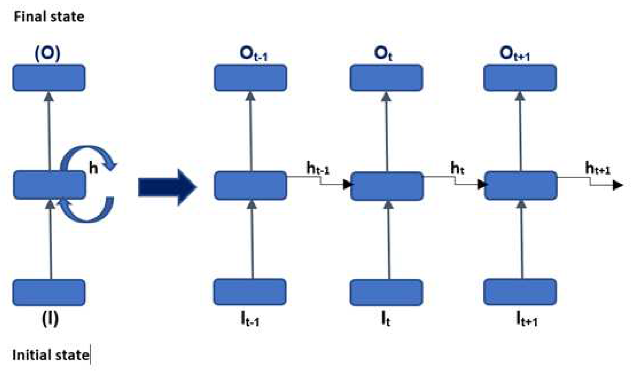
Feed forward neural network does not pass past information retained through memory in time unlike generic RNN units. RNN units have additional advantages like capability to handle sequence data and capability to handle inputs of varying lengths that can be applied to model other types of applications. Architecture of compressed RNN and RNN unfolded in time is shown in
Figure 1.
Practically, the update of the hidden state h
k and final state O
k implemented in equation 1 and 2 [
13]:
Where g is activation function, Wh is weight matrix, bh is bias, by is adjusted bias.
2.3. LSTM Model
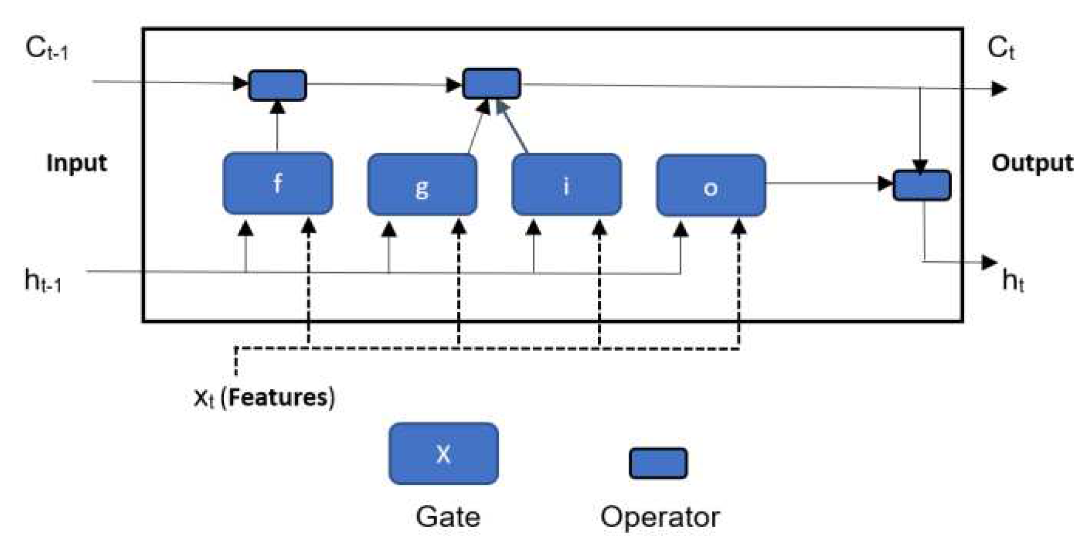
Compared to RNN, LSTM is not only able to keep short-term memories, but also maintain information in memory for long periods of time. LSTM neural network link cause and effects of features and dependant variable respectably by allowing recurrent nets to continue to learn over many time steps [
20]. LSTM neural network contains information in a gated cell. Information can be stored in, written to, or read from a cell via gates that open and close (forget gate, cell candidate, input gate and output gate). x
t is the input features and h
t-1 is the previous hidden state (also referred to as dependent variable) [20, 21]. LSTM cell is shown in
Figure 2. Each gate has weight, bias and activation function. These gates act on the signals to block or pass on information based what they filter with their own sets of weights [
20]. The weights are adjusted by gradient descend method or similar.
2.4. Battery drive cycle Model
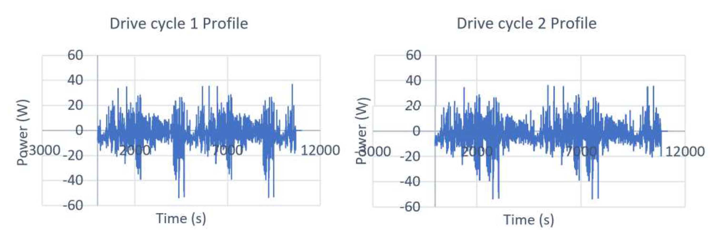
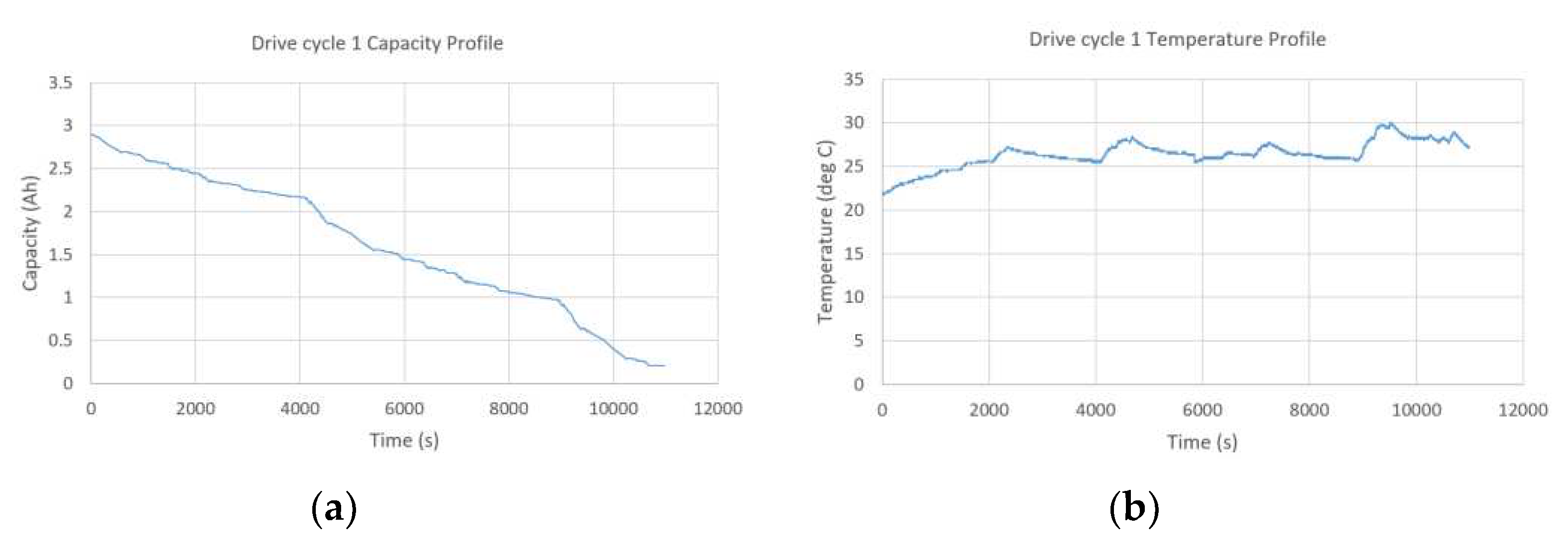
A brand new 2.9Ah Panasonic 18650PF cell dataset is used that is tested in thermal chamber with a 25-amp, 18-volt Digatron Firing Circuits Universal Battery Tester channel. Series of two drive cycles performed are extracted: Cycle 1 and Cycle 2. The drive cycles are datasets for Training and Validation (Cycle 1 and Cycle 2). Cycles 1 and 2 consist of random mixture of US06, HWFET, UDDS, LA92, and Neural Network based drive cycles. The drive cycle profiles are shown in
Figure 3.
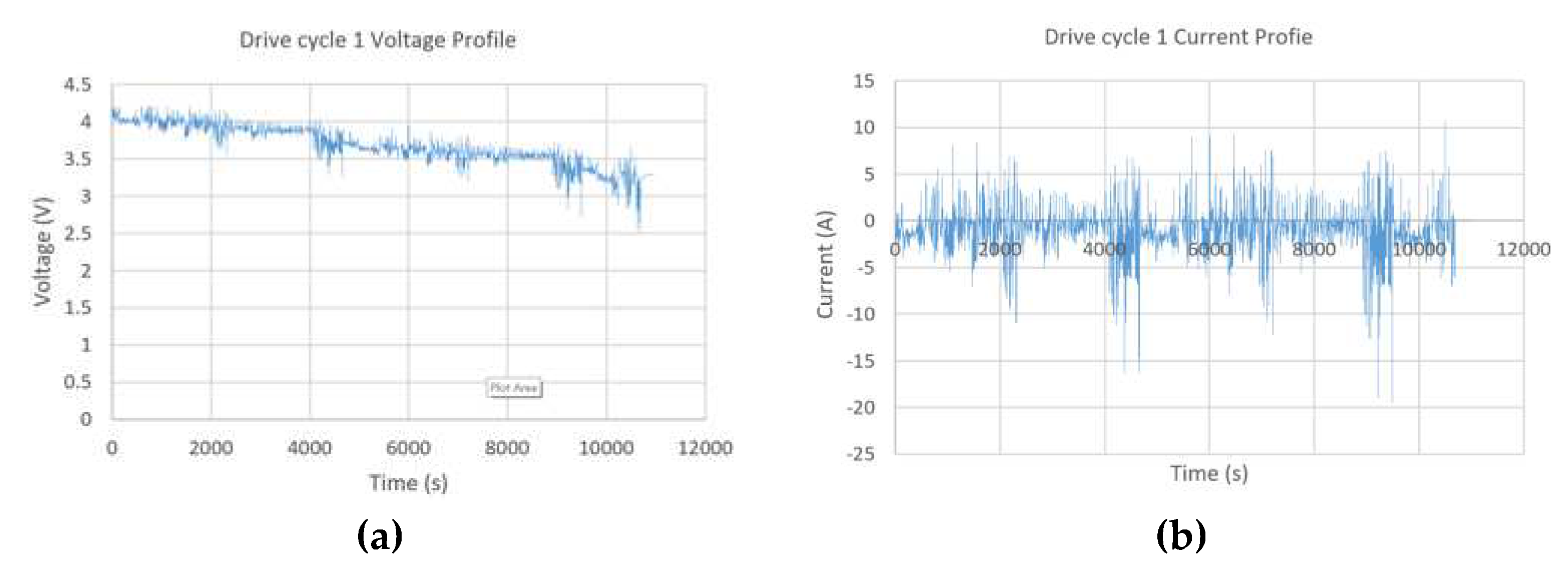
These two cycles were applied on the battery on three algorithms (Generic RNN, LSTM-RNN and Bayesian optimized feedforward neural network) at standard ambient temperatures (25 deg C). For training voltage, current, amp-hour capacity and temperature measurements are applied for online SOC estimation. The profiles for input variables are shown in
Figure 4 and
Figure 5.
3. Methodology
First, the battery discharging load profile data is obtained from battery degradation experiment from the Panasonic 18650PF Li-ion Mendeley datasets. A reasonable sized data samples is extracted from two dataset Cycle 1 and Cycle 2. The reasonable sized data samples are utilized and features {V(k-1), V(k), Ῑ(k-1), T(k-1), T(k), Ah(k)} and dependent variable (SOC) are obtained. For the 3 deep learning algorithms I have specified (learning rate = 0.01, epoch = 300 and hidden neurons = 100 in each hidden layer as per Table 2 in cited journal [
22]) and presumed optimization range of 5-200 neurons. The 3 deep learning algorithms with and without Bayesian optimization counterparts is described below:
3.1. Standard double layered Feedforward
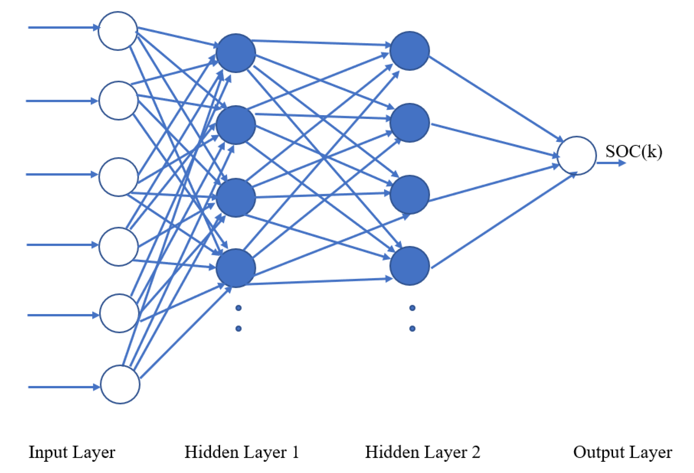
The network diagram of double layered standard feedforward topology is shown in
Figure 6. It has two hidden layers with hidden neurons. The activation functions Sigmoid is used on two hidden layers. The feedforward without optimizations set as 100 neurons in both layers. The feedforward with Bayesian optimization range is set as 5-200 neurons per layer as explained in previous paragraph.
3.2. Standard double layered Feedforward
The network diagram of double layered generic RNN topology is shown in
Figure 7. It has feedback tap delays elements with 100 hidden neurons on each layer for algorithm without Bayesian optimization. The activation functions log-sigmoid is used on two hidden layers and purelin on the output layer. The selection of tap delays (z
-1), hidden neurons and activation functions depends on experimentation and skill of the designer. The weights (w) and bias is updated with training.
3.3. Doubled layered LSTM Model
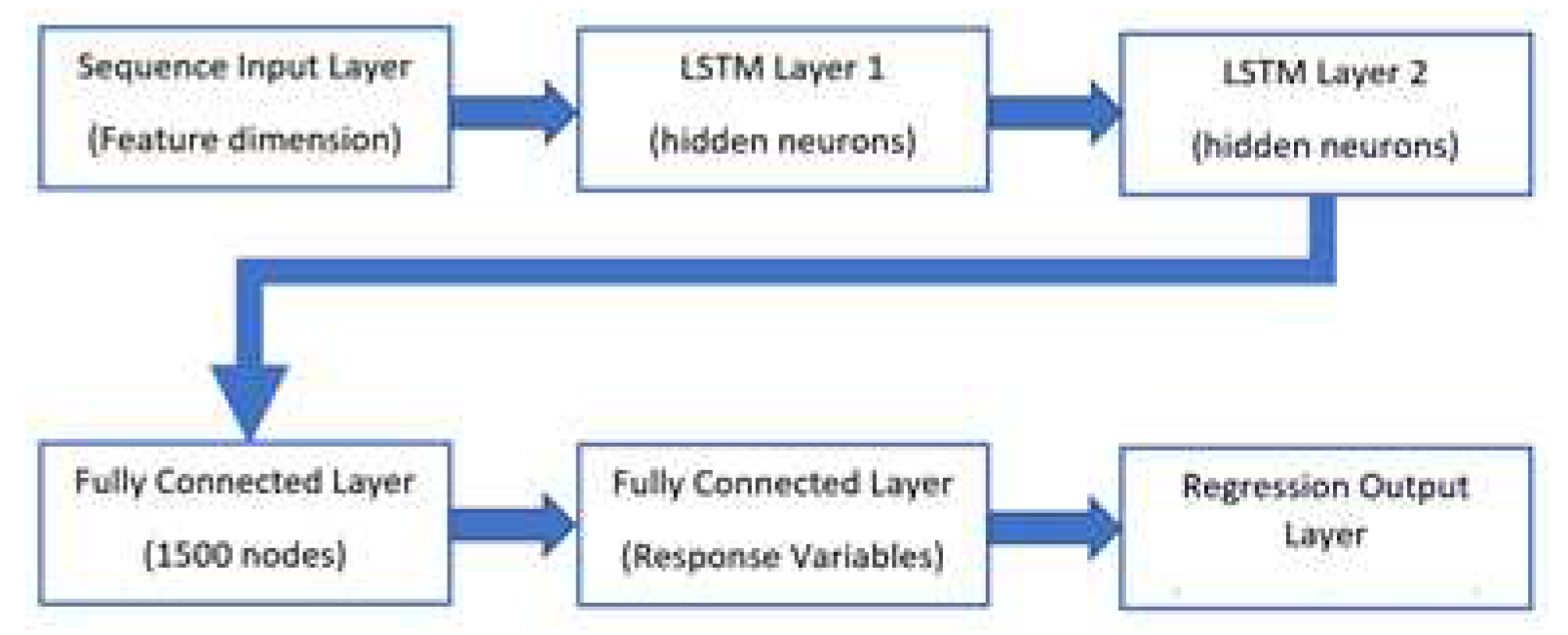
The network diagram of double layered LSTM topology is shown in
Figure 8. The number of nodes is shown inside the bracket. A dropout layer is not used in this design. There are numerous non-linearities within LSTM cells. Therefore, it is unnecessary to add another activation function between the stacked LSTM layers 1 and 2 or between any of the other layers. For LSTM without optimization, 100 neurons are used in each LSTM layer. A fully connected layer of 1500 nodes are used. Second fully connected layer multiplies the input by a weight and then adds a bias similar to neuron in feedforward neural network but without an activation function. A regression layer computes the half-mean-squared-error loss for regression tasks. For typical regression problem like this, a regression layer follows the final fully connected layer. Adam optimizer (adaptive moment estimation) is used in MATLAB to train the weights of network. Training options for Adam is specified. Discussion of trainings options is outside the scope of this journal paper. Allocating number of layers and number of nodes in layers depends on skill of the designer.
3.4. Bayesian optimization for deep learning counterparts
The Bayesian optimization algorithm attempts to minimize a scalar objective function
f(
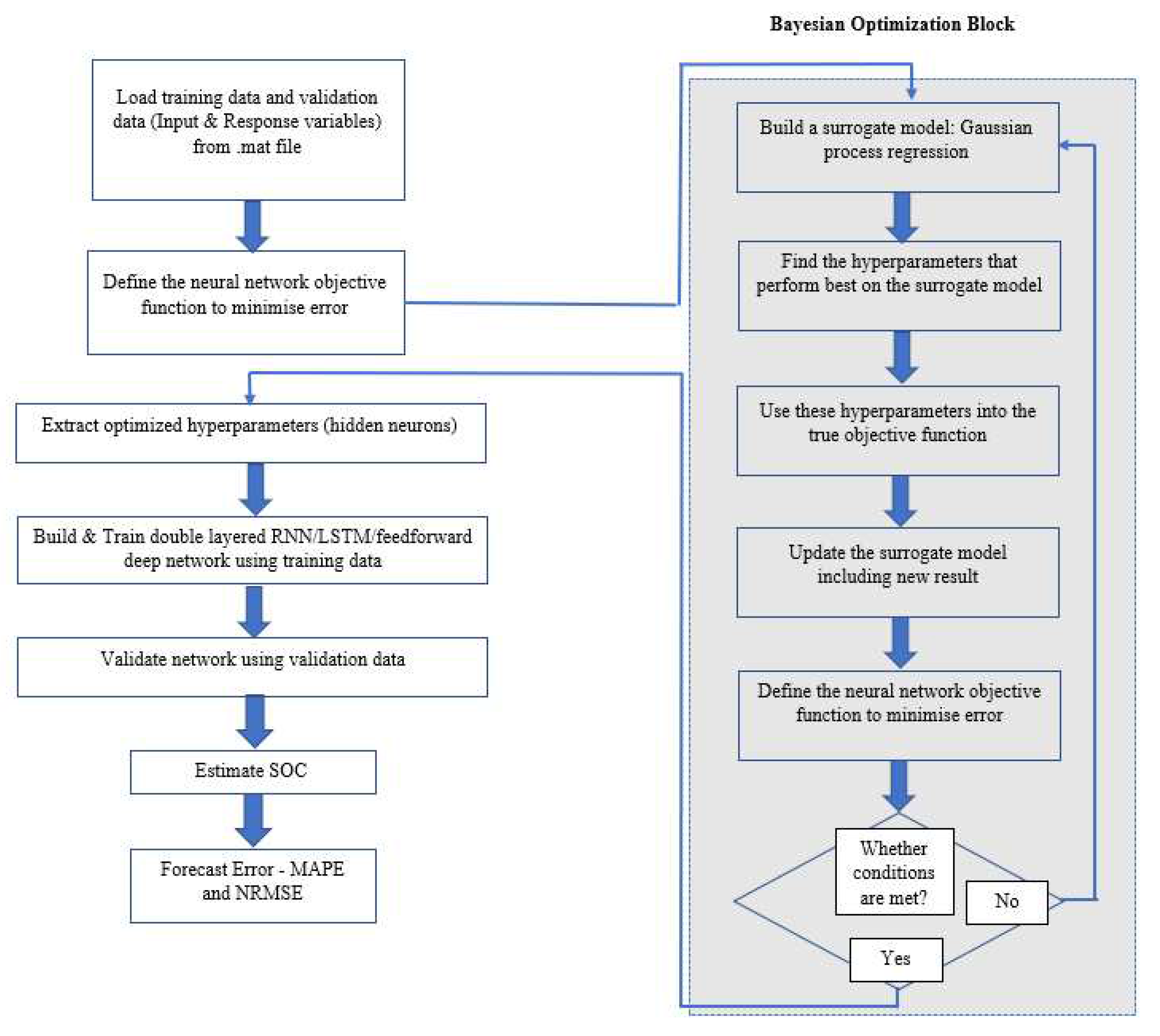
x) for x in a bounded domain. Here f(x) represents a mean squared error (MSE) objective score that is to be minimized and evaluated on the validation set. x symbolizes the set of hyperparameters which produces the minimal value of the respective score. The novel Bayesian optimized deep neural network consist of the following sections as depicted in the flow chart (
Figure 9):
Build a surrogate model of objective function
Find the hyperparameters (hidden neurons in both hidden layers) that perform best on the surrogate model
Use these hyperparameters obtained into the true objective function
Update the surrogate model including new result
Extract hyper parameters and build and train feedforward network based on these hyper parameters.
Instead of manually selecting options to reduce Forecast error, Bayesian hyperparameter optimization is used where different combinations of hyperparameter values (hidden neurons) are selected in the optimization scheme. The optimization range in two layers is 5-200 neurons. This optimization scheme seeks to minimize the model MSE and returns a model with the optimized hyperparameters. It is then possible to use the resulting optimized model as you would use deep trained neural network model without hyperparameter optimization.
4. Results
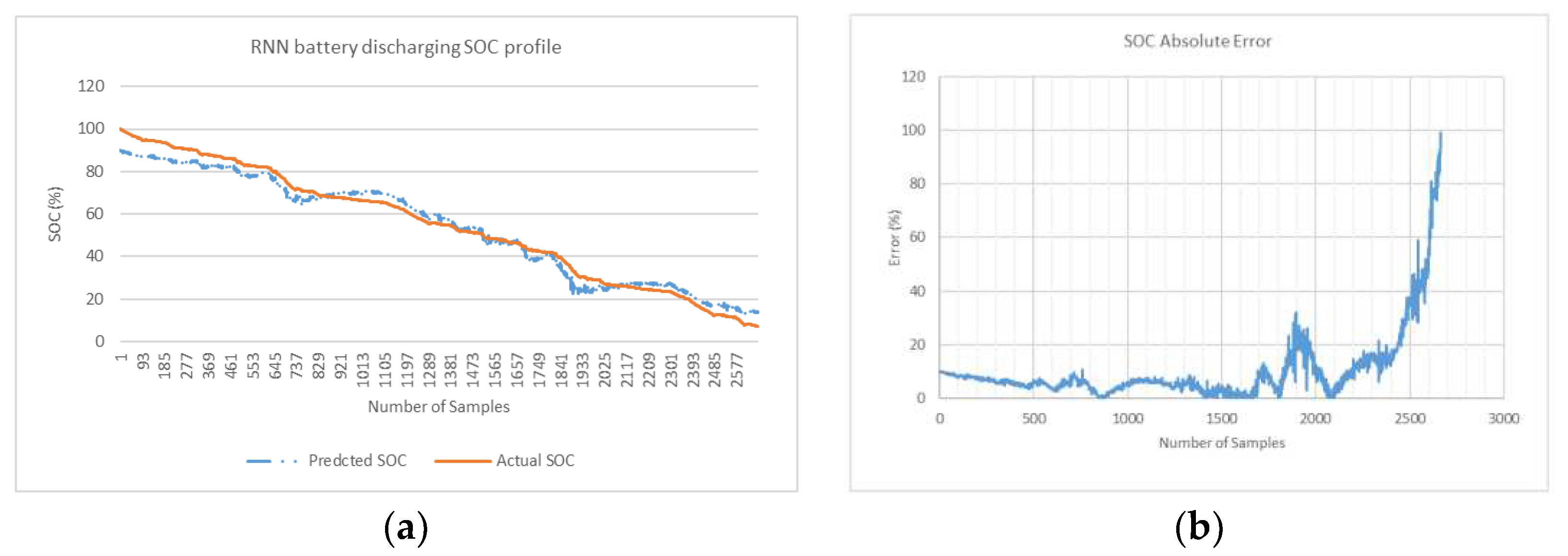
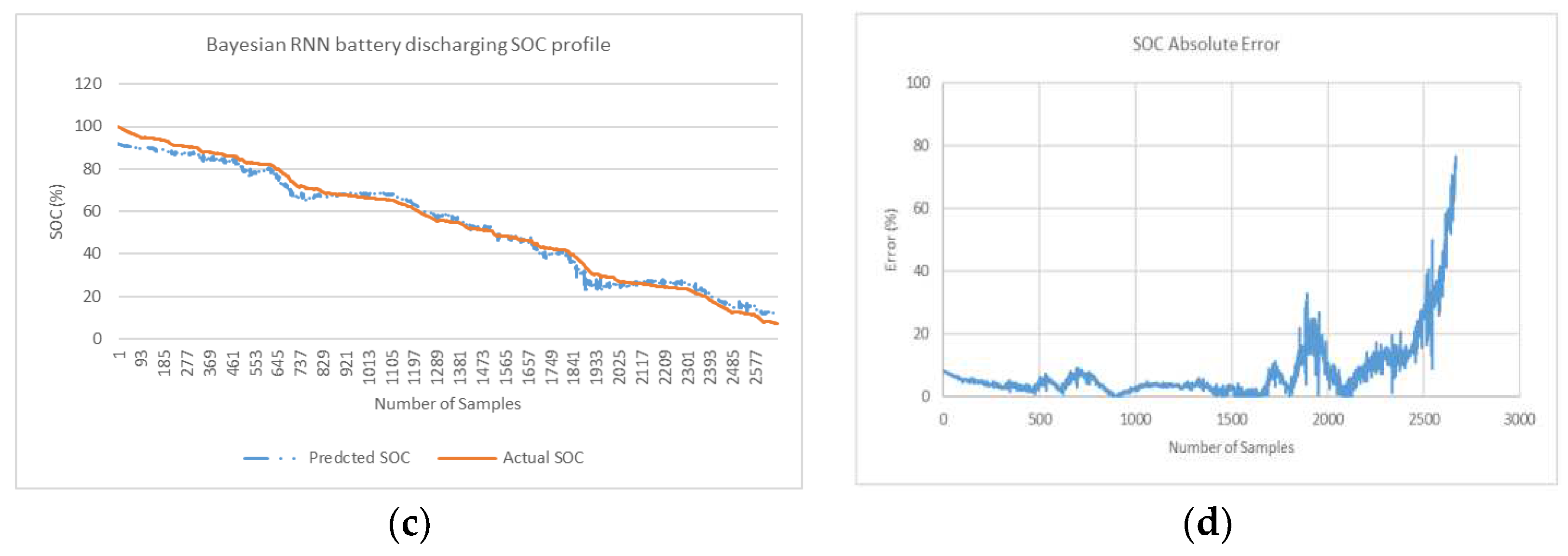
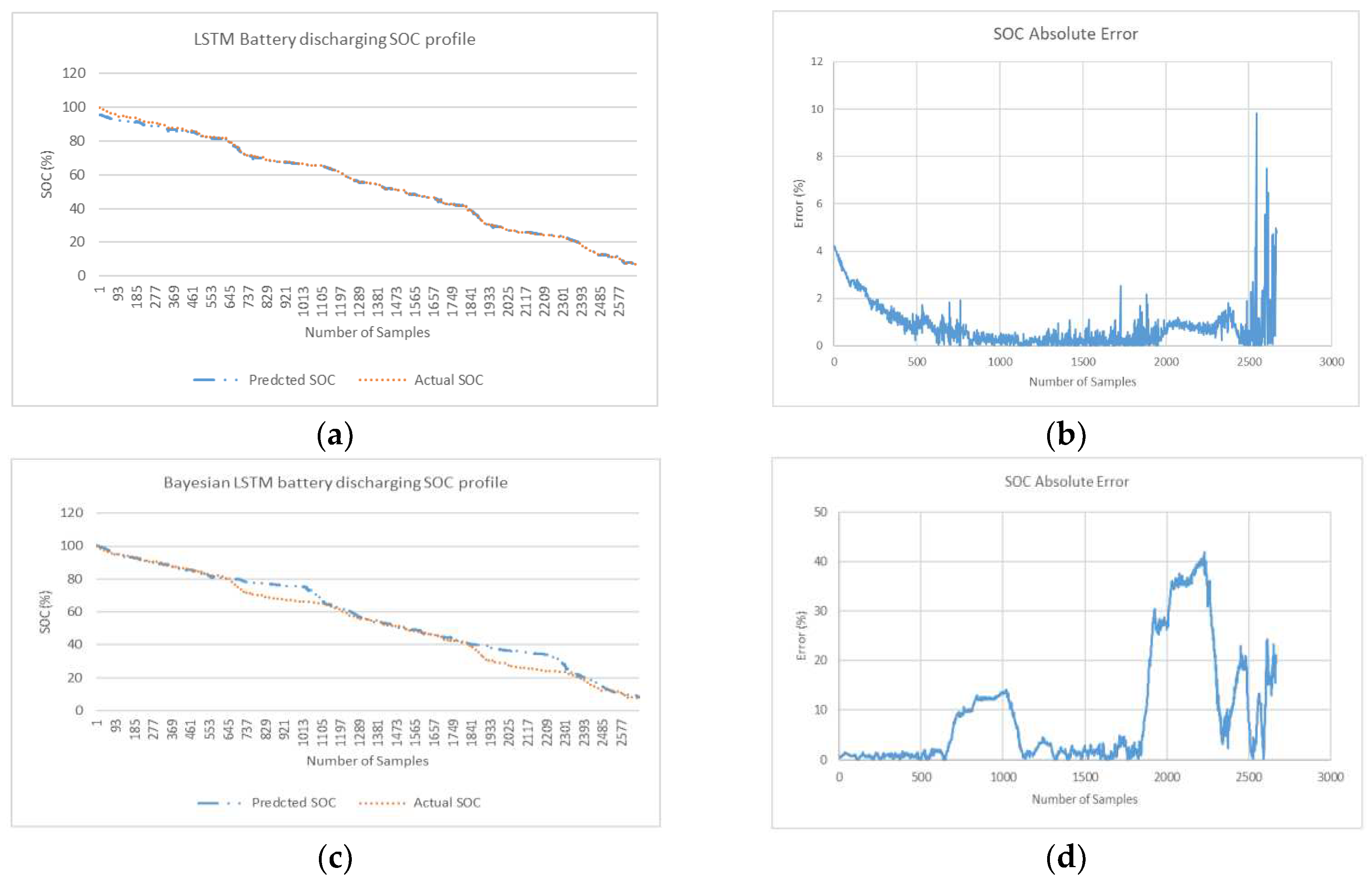
In this section, the network is trained on Drive cycle 1 while validation is performed on Drive cycle 2 (
Figure 3 a & b). This is done to generate SOC prediction curves and SOC absolute error curves. These curves are presented on
Figure 10,
Figure 11 and
Figure 12 for minimum MAPE error profile (when experimented in 3 attempts). The average and minimum error is generated in simulation for 3 attempts is shown in
Table 1. Simulations is conducted for 3 deep learning algorithms without optimization and also for a same 3 algorithms with proposed Bayesian optimization.
NRMSE in
Table 1 gives a relatively high weight to large errors. This means that NRMSE is more suitable when maximum errors are significant. The linear scoring is attributed to MAPE is better indicator at revealing error where minimum error is significant as considered in this research. In MAPE profile, MAPE has components that incorporates both spread term (Absolute SOC Error) and accuracy term (bias) in its formulae. The spread term is divided by actual SOC. In end phases during low values of actual SOC when spread term is high, MAPE indicator is skewed and can give overestimated result. In Bayesian optimized feedforward network, in end phases where there are low values of SOC (for last quarter of fuel gauge figure 11d), the relatively higher error peaks in end phases contribute to higher spread term and overestimation of average MAPE (for 3 profiles). Despite the overestimation of overall MAPE in end phases, it is safe to conclude that Bayesian optimized feedforward algorithm with average MAPE (0.20%) is lowest and is best selection compared with average MAPE for other 5 algorithms considered in
Table 1. From a slightly different perspective, where the results show the minimum MAPE is lowest, feedforward algorithm with optimization is also best selection (min MAPE of 0.06%).
Results is also compiled for algorithms for first three quarter and last quarter of battery discharge samples in
Table 2. In the last remaining quarter of fuel gauge (where actual SOC is less than 25%) feedforward without Bayesian optimization is the best algorithm with lowest average MAPE (MAPE of 0.64%). Overall average MAPE (for example 0.20% Bay Feedforward) is sectioned in first ¾ quarter of cycle (0.10% Bay FF) and last ¼ quarter of cycle (0.64% Bay FF).
5. Conclusion
In this paper, three deep learning neural network algorithms without optimization is compared with identical three algorithm with Bayesian Optimization for battery SOC estimation. The three double layered deep learning algorithms applied are: RNN, LSTM and feedforward network The Bayesian optimization attempts to minimize a scalar objective function for each of the three networks using a surrogate model. The hyperparameters (hidden neurons in both layers) are extracted using surrogate model. Furthemore the hyperparameters are build and trained for first drive cycle. Validation is done for second drive cycle. As per explaination in results section MAPE indicator is preferred over NRMSE indicator. However, overall MAPE is a overetimated indicator in the context of results shown in figures 9, 10 and 11 and arguments presented in results section thereof. Despite the overestimation of overall MAPE in end phases, it is safe to conclude that Bayesian optimized feedforward algorithm with average MAPE (0.20%) is lowest and is best selection compared with average MAPE for other 5 deep learning algorithms. From a slightly different perspective, where results show the minimum MAPE is lowest, feedforward algorithm with optimization is best selection (min MAPE of 0.06%). In the last remaining quarter of fuel gauge (where actual SOC is less than 25%) feedforward with optimization is still the best selection with low average MAPE error of 0.64%.
References
- Aryal, A., M. Hossain, and K. Khalilpour. A Comparative study on state of charge estimation techniques for Lithium-ion Batteries. in 2021 IEEE PES Innovative Smart Grid Technologies-Asia (ISGT Asia). 2021. [CrossRef]
- Feng, X.; et al. State-of-charge estimation of lithium-ion battery based on clockwork recurrent neural network. Energy 2021, 236, 121360. [Google Scholar] [CrossRef]
- Wang, Q.; et al. Least squares support vector machine for state of charge estimation of lithium-ion battery using gray wolf optimizer. Journal of Physics: Conference Series. 2021. IOP Publishing. [CrossRef]
- Ismail, M.; et al. Battery state of charge estimation using an Artificial Neural Network. in 2017 IEEE Transportation Electrification Conference and Expo (ITEC). 2017. IEEE. [CrossRef]
- Zhang, C.-W.; et al. State of charge estimation of power battery using improved back propagation neural network. Batteries 2018, 4, 69. [Google Scholar] [CrossRef]
- Chaoui, H.; Ibe-Ekeocha, C.C. State of charge and state of health estimation for lithium batteries using recurrent neural networks. IEEE Transactions on vehicular technology 2017, 66, 8773–8783. [Google Scholar] [CrossRef]
- Chemali, E.; et al. Long short-term memory networks for accurate state-of-charge estimation of Li-ion batteries. IEEE Transactions on Industrial Electronics 2017, 65, 6730–6739. [Google Scholar] [CrossRef]
- Chemali, E.; et al. State-of-charge estimation of Li-ion batteries using deep neural networks: A machine learning approach. Journal of Power Sources 2018, 400, 242–255. [Google Scholar] [CrossRef]
- Orr, B. The Exploding and Vanishing Gradients Problem in Time Series. 2020, Towards Data Science.
- Shewalkar, A. Performance evaluation of deep neural networks applied to speech recognition: RNN, LSTM and GRU. Journal of Artificial Intelligence and Soft Computing Research 2019, 9, 235–245. [Google Scholar] [CrossRef]
- Shi, Z.; et al. A long short-term memory network for online state-of-charge estimation of li-ion battery cells. in 2020 IEEE Transportation Electrification Conference & Expo (ITEC). 2020. [CrossRef]
- Wu, J.; et al. Hyperparameter optimization for machine learning models based on Bayesian optimization. Journal of Electronic Science and Technology 2019, 17, 26–40. [Google Scholar]
- Yang, F.; et al. State-of-charge estimation of lithium-ion batteries based on gated recurrent neural network. Energy 2019, 175, 66–75. [Google Scholar] [CrossRef]
- Zhang, S.; Liu, Z.; Su, H. A Bayesian Mixture Neural Network for Remaining Useful Life Prediction of Lithium-Ion Batteries. IEEE Transactions on Transportation Electrification, 2022. [CrossRef]
- Xu, S.; Zhou, F.; Liu, Y. A hybrid method for lithium-ion batteries state-of-charge estimation based on gated recurrent unit neural network and an adaptive unscented Kalman filter. Journal of Electrochemical Energy Conversion and Storage 2022, 19, 031005. [Google Scholar] [CrossRef]
- Zhang, S.; et al. A data-driven coulomb counting method for state of charge calibration and estimation of lithium-ion battery. Sustainable Energy Technologies and Assessments 2020, 40, 100752. [Google Scholar] [CrossRef]
- Chen, G.; et al. Electrochemical-distributed thermal coupled model-based state of charge estimation for cylindrical lithium-ion batteries. Control Engineering Practice 2021, 109, 104734. [Google Scholar] [CrossRef]
- Ndeche, K.C.; Ezeonu, S. O. Implementation of Coulomb Counting Method for Estimating the State of Charge of Lithium-Ion Battery. Physical Science International Journal 2021, 25, 1–8. [Google Scholar] [CrossRef]
- Hu, X.; Li, S.E.; Yang, Y. Advanced machine learning approach for lithium-ion battery state estimation in electric vehicles. IEEE Transactions on Transportation electrification 2015, 2, 140–149. [Google Scholar] [CrossRef]
- Nicholson, C. A Beginner's Guide to LSTMs and Recurrent Neural Networks. 2020.
- Documentation, M. Long Short-Term Memory Networks. 2022: MAthWorks Inc.
- Koutsoukas, A.; et al. Deep-learning: investigating deep neural networks hyper-parameters and comparison of performance to shallow methods for modeling bioactivity data. Journal of cheminformatics 2017, 9, 1–13. [Google Scholar] [CrossRef] [PubMed]
- Arifuzzaman, M.; et al. Application of artificial intelligence (ai) for sustainable highway and road system. Symmetry 2020, 13, 60. [Google Scholar] [CrossRef]
|
Disclaimer/Publisher’s Note: The statements, opinions and data contained in all publications are solely those of the individual author(s) and contributor(s) and not of MDPI and/or the editor(s). MDPI and/or the editor(s) disclaim responsibility for any injury to people or property resulting from any ideas, methods, instructions or products referred to in the content. |
© 2023 by the authors. Licensee MDPI, Basel, Switzerland. This article is an open access article distributed under the terms and conditions of the Creative Commons Attribution (CC BY) license (http://creativecommons.org/licenses/by/4.0/).
